revtex4-2Repair the float

Quantum Convolutional Neural Network for Phase Recognition in Two Dimensions

Abstract

Quantum convolutional neural networks (QCNNs) are quantum circuits for recognizing quantum phases of matter at low sampling cost and have been designed for condensed matter systems in one dimension. Here we construct a QCNN that can perform phase recognition in two dimensions and correctly identify the phase transition from a Toric Code phase with $\mathbb{Z}_{2}$-topological order to the paramagnetic phase. The network also exhibits a noise threshold up to which the topological order is recognized. Our work generalizes phase recognition with QCNNs to higher spatial dimensions and intrinsic topological order, where exploration and characterization via classical numerics become challenging.

The remarkable progress in quantum computing technologies has led to the development of noisy intermediate-scale quantum (NISQ) computers [1] as well as to proof-of-principle demonstrations of quantum error correction [2, 1], fault-tolerant gate sets [3] and algorithms [4]. As a consequence, the output quantum states of quantum computers and simulations are becoming too complex to characterize them with classical computers. While many local properties of quantum states can be efficiently characterized using shadow tomography [5], the characterization of global properties remains an open challenge.

The direct processing of quantum data on quantum computers offers a potential solution to this problem, where recent developments include quantum autoencoders [6, 7], quantum principle component analysis [8], certification of Hamiltonian dynamics [9, 10], and quantum reservoir processing [11]. Particularly promising are quantum neural networks that use parameterized quantum circuits, measurement and feed-forward to characterize large amounts of quantum data [12, 13, 14, 15, 16].

A central field for applications of quantum computing is condensed matter physics, where the characterization of quantum states is of central importance. In particular, the classification of phases of matter [17, 18] is a key requirement for understanding strongly correlated materials [19]. While phases of matter in one-dimensional systems are well-understood thanks to accurate classical numerical simulations [20], two- and higher-dimensional systems are notoriously hard to simulate on classical computers due to the exponential growth of Hilbert space with the number of particles [21, 22].

Topological many-body phases of matter have been prepared on quantum computers using unitary quantum circuits [23] as well as measurement and feed-forward [24, 25], thus opening a new way for their investigation. The characterization of these topological phases however remains challenging due to the absence of local order parameters and because other characteristic quantities, such as fidelity susceptibility and entanglement, are hard to measure. Previous approaches to address this challenge include classical machine learning techniques applied to data from classical numerical simulations [26, 27, 28] and classical shadows [29]. Topological phases have also been detected from data measured in an experiment by combining techniques from quantum error correction and renormalization-group flow [30], which is a well-established method for the classification of phases of matter [19]. Nonetheless, these approaches are limited by the large amounts of data required for describing quantum states on classical computers.

Quantum convolutional neural networks (QCNNs) have been proposed to substantially reduce the sample complexity of recognizing symmetry-protected topological phases [13, 31] in one dimension and were shown to uncover characteristic properties of such phases from training data via supervised learning [13, 32, 33]. There are explicitly constructed QCNNs that are robust against errors in quantum data [34] and therefore implementable on a superconducting quantum processor under NISQ conditions [35]. However, these QCNNs have only been applied to one-dimensional systems, which can be accurately simulated on classical numerical computers. The extension of QCNNs to two- and higher-dimensional systems, where quantum computers can potentially provide a computational advantage, has remained unexplored.

Here, we address this open challenge by generalizing QCNNs to detect $\mathbb{Z}_{2}$-topological order in two-dimensional spin arrays. We analytically construct a QCNN inspired by quantum error correction and Multiscale Entanglement Renormalization Ansatz [36]. Using matrix-product-state simulations, we show that the QCNN recognizes the topological phase of the Toric Code Hamiltonian in a magnetic field from a topologically trivial magnetic phase. In contrast to methods based on the processing of measurement data on a classical computer [30], the QCNN precisely identifies the critical value of the magnetic field where the Toric Code undergoes the phase transition. Moreover, the QCNN output is robust against incoherent errors below a threshold error probability allowing for the application of the QCNN under NISQ conditions on current quantum computers.

QCNNs are phase recognition circuits, which are an analog of classical Convolutional Neural Networks (CNNs). A QCNN can be written as a unitary of the form [13, 35, 31, 34],

$$U_{\mathrm{QCNN}}=U_{\mathrm{FC}}\prod_{j}^{d}U_{\mathrm{CP}}^{(j)}\,,$$ (1)

where the unitary $U_{\mathrm{CP}}^{(j)}$ represents a combination of a convolutional and a pooling layer, $d$ is the number of subsequent layers and the unitary $U_{\mathrm{FC}}$ is a fully connected layer that prepares the output. Subsequently, the output qubit(s) are measured. For the $j^{\mathrm{th}}$ layer in the QCNN structure, we specifically define the unitary $U_{\mathrm{CP}}^{(j)}$ as $U_{\mathrm{CP}}^{(j)}=U_{\mathrm{P}}^{(j)}U_{\mathrm{C}}^{(j)}(U_{\mathrm{C}}^{(j-1)})^{\dagger}$, where $U_{\mathrm{P}}^{(j)}$ is the unitary implemented by the pooling procedure, $U_{\mathrm{C}}^{(j)}$ the convolution of the current layer and $(U_{\mathrm{C}}^{(j-1)})^{\dagger}$ the adjoint of the convolution of the preceding layer $j-1$.

If we construct the convolutional layers from Clifford gates and the pooling procedure via single qubit Pauli-operations that are controlled by the results of measurements of other qubits, we can shorten the QCNN circuit dramatically by pushing $U_{\mathrm{C}}^{(j)}$ through the pooling circuit $U_{\mathrm{P}}^{(j)}$ [35, 37]. We then obtain a modified pooling layer $\tilde{U}_{\mathrm{P}}^{(j)}$ and subsequently cancel all convolutions except the first one, such that we can write the QCNN unitary as

$$U_{\mathrm{QCNN}}=U_{\mathrm{FC}}\left(\prod_{j}^{d}\tilde{U}_{\mathrm{P}}^{(j)}\right)U_{\mathrm{C}}^{(0)}\,.$$ (2)

Our algorithm is based on the fact that topological order is robust to local perturbations [17]. Hence, one can define characteristic states $\ket{\psi_{i}}$ for each phase of the Hilbert space and treat other states of the same phase as characteristic states masked by unitary perturbations $\ket{\phi_{j}}=U_{j,\mathrm{E}}\ket{\psi_{j}}$ that we identify as errors. If one can recover the characteristic state by removing these errors, one has successfully identified the corresponding phase. In Figure 1 we sketch such a phase space and the recovery of the reference state by using error correction. The explicit structure of our QCNN can be found in the supplementary material.

[width=1]standalone/RGflow1dim

Figure 1: Schematic of phase recognition via a QCNN for two phases with characteristic states $\ket{\psi_{1}}$ and $\ket{\psi_{2}}$. Other states $\ket{\phi_{j}}$ in the respective phases can be generated by local unitary perturbations $\ket{\phi_{j}}=U_{j,\mathrm{E}}\ket{\psi_{j}}$ and the phase can for each input state be identified by undoing the respective perturbation $U_{j,\mathrm{E}}$ via sufficient error correction.

At each qubit layer $l$, we can generate an output by ‘measuring’ the qubits in the computational basis,

$$M^{l}_{\mathrm{QCNN}}=\dfrac{2}{N_{l}}\left(\sum_{j=1}^{N_{l}}m_{j}\right)-1\,$$ (3)

where $m_{j}\in\{-1,1\}$ is the measurement outcome of qubit $j$ and $N_{l}$ the number of qubits in layer $l$. Specifically, we implement the controlled Pauli gates of the pooling circuit classically on the bit string of computational basis measurements for all qubits and update the bit string accordingly. As these operations are performed in classical post-processing, the ’measurements’ correspond to simply recording the classical data. For our QCNN, $M^{l}_{\mathrm{QCNN}}$ as defined in Equation 3, will have the following averages over a large number of samples

$$\braket{\mathrm{QCNN}}\coloneqq\braket{M^{l}_{\mathrm{QCNN}}}=\begin{cases}1&\text{if topological phase}\\ 0&\text{if non-topological phase}\,.\end{cases}$$ (4)

We consider the two-dimensional Toric Code [38] with periodic boundary conditions as a natural candidate for exploring QCNNs for two-dimensional systems as it shows intrinsic $\mathbb{Z}_{2}$-topological order [38]. As previous approaches to QCNNs have been restricted to one-dimensional settings [13, 35, 33, 37], the Toric Code lends itself ideally to expand the field of QCNNs to higher dimensional systems. The Toric Code is a two-dimensional square lattice with the qubits located on its edges. For exploring its condensed matter physics, it can be described by the Hamiltonian

$$H_{\mathrm{TC}}=-\sum_{i}A_{i}-\sum_{i}B_{i}$$ (5)

with the plaquette operators $A_{i}=\prod_{i=1}^{4}X_{i}$ and the star operators $B_{i}=\prod_{i=1}^{4}Z_{i}$, where $X_{i}$ ($Z_{i}$) is the Pauli-X(Z) operator on qubit $i$, see Figure 2.

[width=]standalone/QCNN_diagram2

Figure 2: QCNN structure. The first lattice on the input side shows the Toric Code lattice with dimension $d=4\times 4$, which is periodic in vertical and horizontal direction. The qubits on the respective sublattices are represented by gray (horizontal edges) and green circles (vertical edges). Examples of plaquette ($A_{i}$) and vertex ($B_{i}$) operators are highlighted in blue and orange. The circuit of the convolution maps the stabilizers of the input lattice to measurements on individual qubits of the respective colors, i.e. blue qubits carry the measurement of the plaquette stabilizer that is anchored on the qubits to their left and orange qubits carry the information of stabilizers to their right. This convolution evolves error patterns on the input state and brings them into a form that can be corrected by the local operations in the pooling if the input was in the topological phase. Iterated pooling procedures reduce the lattice dimension (green squares) with every step until only two output qubits are left (green dots) and read out.

If the Toric Code is exposed to external magnetic fields of sufficient strength, it will undergo a second-order phase transition [39, 40] between the topologically ordered and a paramagnetic phase. To explore these regimes, we modify Equation 5 to include applied magnetic fields in X- and Z-direction with strengths $h_{X}$ and $h_{Z}$,

$$H_{\mathrm{mag}}=H_{\mathrm{TC}}-h_{Z}\sum_{i}^{N}Z_{i}-h_{X}\sum_{i}^{N}X_{i}\,.$$ (6)

The concept of the QCNN that we apply to (noisy) ground states of this model is sketched in Figure 2 and its detailed description can be found in the supplementary material. The QCNN we here propose is capable of detecting the topologically ordered phase with high accuracy, that is, the QCNN’s output converges to 1 if the input state is in the topological phase and to 0 otherwise.

To evaluate the performance of our QCNN we carried out several numerical simulations. For investigating the scaling of its performance with increasing depth $d$, we need to consider large system sizes, for which we use Matrix Product State (MPS) simulations [41] to approximate ground states of the Hamiltonian Equation 6 and classical simulations of Clifford gates on Pauli strings for exploring the effects of incoherent Pauli noise.

We first test the QCNN on ground states of $H_{\textrm{mag}}$ with a magnetic field in Z-direction, $h_{X}=0$ in Equation 6. We show the details of our MPS implementation in the supplementary material. With our implementation, we can generate the phase diagram as shown in Figure 3, where we consider field strengths $0\leq h_{Z}\leq 1$. From iDMRG simulations for our cylindrical lattice, we determine the phase boundary at $h_{Z}^{*}=0.34$ as a peak in the second derivative $d^{2}E/dh_{Z}^{2}$ of the ground state energy with respect to $h_{Z}$, which we mark in the phase diagram. The plot shows that the QCNN output $\braket{M^{l}_{\mathrm{QCNN}}}$, c.f. Equation 3, shows a transition at this expected point up to the sample resolution. Additionally, the sharpness of the transition increases with the layer number in the sense that the absolute value of the gradient of $\braket{M^{l}_{\mathrm{QCNN}}}$ increases, which makes the transition in the output more step-like with an increasing number of pooling layers. This shows the successful recognition of the topological phase by the QCNN.

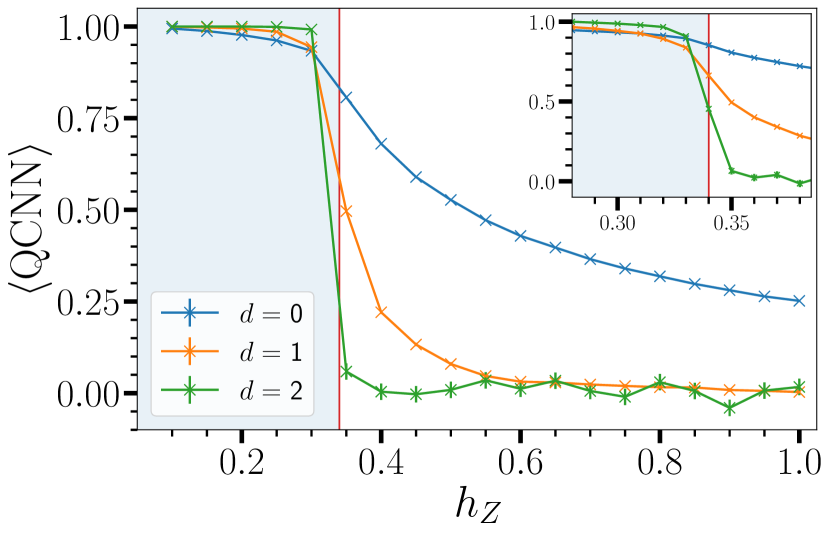
Figure 3: QCNN output for a variation of the magnetic field strength $h_{Z}$, where $h_{X}=0$, and for different depths $d$ of the QCNN, corresponding to the number of pooling layers $U_{P,j}$. Each data point represents 2000 samples from the MPS representation of the corresponding ground state. The shaded region corresponds to the topologically ordered phase and the vertical line to critical magnetic field strength $h^{*}_{Z}=0.34$. The insert shows the output for different samples with higher resolution around the phase transition, which are calculated with a bond dimension of $\chi=1500$, whereas for the main plot, the bond dimension is $\chi=1250$. For all samples, we observe increased steepness at the phase transition in the QCNN output with increasing QCNN depth corresponding to greater precision in the phase recognition.

Next, we test the QCNN on ground states of $H_{\textrm{mag}}$ with magnetic field in both X- and Z-direction. First, we consider constant $h_{X}=0.1$ leading to a non-vanishing probability of error syndromes $B_{i}=-1$ on vertices and thus $M_{\mathrm{QCNN}}^{0}<1$, see Figure 4. Second, we consider the transition into the trivial phase driven by perturbations in both X- and Z-directions for $h_{X}=h_{Z}=h$ [42]. The QCNN output rapidly decreases with increasing depth $d$ above the multicritical point $h=0.35$, see Figure 4b. This provides clear evidence that the QCNN recognizes the phase transition also for these cases.

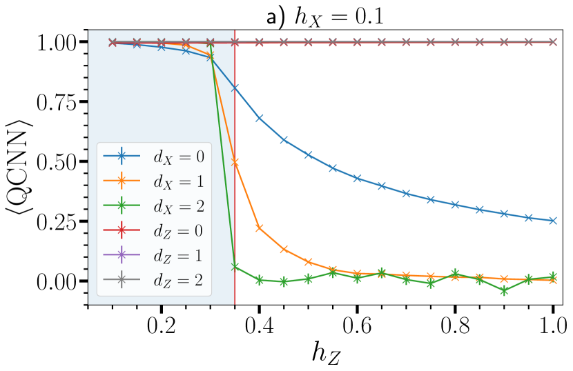
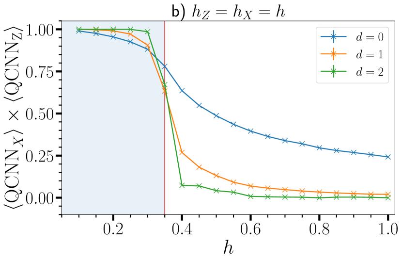
Figure 4: a) Output of the QCNN for the MPS samples under a variation of $h_{Z}$ in the presence of a weak magnetic field in X-direction with $h_{X}=0.1$ with a bond dimension of $\chi=1250$. The output is displayed for simultaneous pooling in the X(Z)-basis for the corresponding QCNN depth $d_{X}$($d_{Z}$). The phase transition for $h_{Z}$ is correctly recognized in the presence of a field in X-direction. Furthermore, the output of the pooling layers $d_{Z}$ quickly converges to unity due to the weak $h_{X}=0.1$. b) Detection of the multicritical point [42] in the presence of X- and Z-field with $h=h_{X}=h_{Z}$ for a bond dimension of $\chi=1500$. We take the product of the pooling in the X- and Z-basis for each QCNN layer to show the combined phase recognition along the multicritical line $h_{X}=h_{Z}$. A split plot can be found in the supplementary material in Figure 10.

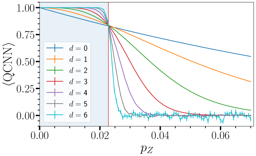
Figure 5: QCNN output for incoherent Pauli noise perturbing the Toric Code ground state as in Equation 7. Via tracking the evolution of Pauli strings on the lattice under the convolution and the pooling layers we can classically simulate the QCNN output for large system sizes. For this plot, we calculate the results for about 9.6 Million qubits, which allows us to employ more pooling layers compared to the MPS samples. As for the case of the magnetic field, we find a transition in the QCNN output that becomes more pronounced with increasing depth of the QCNN. The red vertical line marks the error threshold of $p_{\mathrm{th}}=2.28\%$.

We also test whether our QCNN is able to recognize the topological phase in the presence of incoherent noise. We do this by considering the Toric Code ground state perturbed by Pauli noise. Specifically, we apply random Pauli noise to each individual qubit in the form of the error channel

$$\rho=\mathcal{E}(\ket{\psi}\bra{\psi})=\sum_{l=0}^{m}K_{l}\ket{\psi}\bra{\psi}K_{l}^{\dagger}\,,$$ (7)

with $K_{l}\in\{\sqrt{p_{\mathds{1}}}\mathds{1},\,\sqrt{p_{X}}X,\,\sqrt{p_{Z}}Z\}^{\otimes N}$ to the input qubits. $p_{X}$($p_{Z}$) is the probability for a Pauli-X(Z) error on any single qubit and $p_{\mathds{1}}=1-p_{X}-p_{Z}$. A Pauli-Y error occurs as the product of a Pauli-X and a Pauli-Z error on the same qubit. As the QCNN only consists of Clifford and controlled Pauli gates, we can then subsequently track the evolution of the Pauli error strings on the lattice under the operations of the QCNN. It is sufficient to employ the following gate identities $X_{j}=H_{j}Z_{j}H_{j}$, $\textrm{CNOT}_{i,j}X_{i}=X_{i}X_{j}\textrm{CNOT}_{i,j}$ and $\textrm{CNOT}_{i,j}Z_{j}=Z_{i}Z_{j}\textrm{CNOT}_{i,j}$, where $H_{j}$ is the Hadamard gate on qubit $j$ and $\textrm{CNOT}_{i,j}$ applies a Pauli $X$ on qubit $j$ conditioned on qubit $i$.

We present results for the QCNN output, Equation 3, for cases where the input state is the reference state of the topological phase, i.e. a ground state of $H_{\mathrm{TC}}$ as in Equation 5 perturbed by Pauli-Z noise in Figure 5, which shows a transition in the QCNN output over the Pauli-Z error probability $p_{Z}$. The absolute value of the gradient at the transition point increases with the number of QCNN layers. This corresponds to the desired behavior of the QCNN as the confidence of the QCNN output increases with additional layers. In the supplementary material, we also show results for simultaneous Pauli-Z and Pauli-X noise.

Lastly, we tested the phase recognition capability of the QCNN for Toric Code ground states of varying magnetic field strength, that are perturbed by Pauli noise. To this end, we reevaluate the samples from Figure 3 and additionally apply the Pauli noise channel Equation 7 to them. Here, we find that the QCNN retains the ability to recognize the phase until the Pauli noise threshold of $p_{\mathrm{th}}=2.28\%$ is reached, which we deduce from Figure 5. In Figure 6 we plot the results for a demonstrative sample of $p_{X}=p_{Z}\in\{0.0225,\,0.03,\,0.045,\,0.1\}$.

The plots of Figure 6 show that incoherent Pauli errors have, as expected, a significant influence on the QCNN output for the Toric Code ground states as soon as the error rates reach the threshold $p_{\mathrm{th}}$. Up to the threshold, the QCNN output behaves similarly as in Figure 3. However, for $p_{X}=p_{Z}=2.25\%$ the output curve for layer 1 drops below the curve for layer 0. Since $\braket{M^{l}_{\mathrm{QCNN}}}$ depends on the error rate on the lattice at layer $l$, this indicates that the density of errors has increased with the first pooling layer. Such behavior is expected as the error rate is close to the threshold. In this case, the number of errors removed by the first pooling layer is smaller than the reduction in the total number of qubits and the errors can only be cleared sufficiently with the subsequent pooling layer. This behavior also starts to become apparent in the second pooling layer for larger error rates and for our last test with $p_{X}=p_{Z}=10\%$ the error density after the second pooling layer even increases beyond the density after the first layer.

The phase recognition continues to agree with the ground states in the absence of Pauli-noise up to $p_{X}=p_{Z}=3\%$, where the input states up to the phase transition are more likely to be characterized correctly since the average QCNN output $\braket{\mathrm{QCNN}}$ rests above $50\%$ in the topological phase. In our tests, we find topological input states that are falsely characterized as trivial for $p_{j}>3\%(j=X,Z)$ and for strong Pauli noise at $p_{X}=p_{Z}=10\%$ no input state ensemble is characterized as topological. This behavior is expected as the correlation length of the syndromes of the Pauli errors becomes so long compared to the error correction capabilities of the QCNN, that the topological character of the input states remains masked.

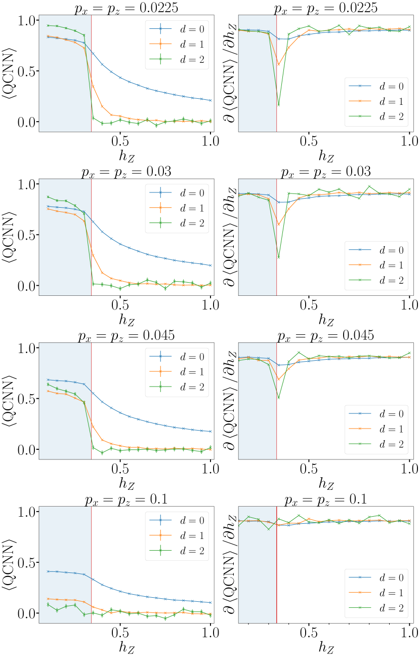
Figure 6: QCNN output for the MPS samples over the magnetic field strength $h_{Z}$ under the influence of incoherent Pauli errors with rate $p_{X}=p_{Z}\in\{0.0225,\,0.03,\,0.045,\,0.1\}$ with bond dimension $\chi=1250$. On the right side, we plot the gradient of the QCNN output to show how the increasing noise influences the detected point of steepest change. We observe that even for noise that surpasses the Pauli noise threshold $p_{\mathrm{th}}=2.28\%$ the point of steepest change is still correctly identified at the phase transition $h_{Z}^{*}=0.34$ up to the resolution of our samples. In the bottom row, we show that for strong Pauli noise of $p_{X}=p_{Z}=0.1$, the ability to recognize the phase transition is lost.

In conclusion, we generalized QCNNs to two-dimensional systems and showed that they recognize the topological phase of the Toric Code. The QCNN output is robust against errors below a threshold probability allowing for their realization on current quantum computers under NISQ conditions. Furthermore, all pooling layers can be efficiently performed in classical post-processing to facilitate the QCNN implementation with restricted circuit depths on NISQ devices. In future research, one can further investigate the quantum error correction procedure in the pooling layers to increase the error threshold and enhance the phase detection by a faster convergence to a step function with the number of pooling layers. The implementation of the convolutional layer as a quantum circuit opens the way for the efficient processing of quantum data with reduced sample complexity [35, 34]. We expect that our work motivates the exploitation of QCNNs for the characterization of less-understood quantum phases of matter such as symmetry-enriched topological order [43] and quantum spin liquids [18]. Implementing pooling layers as quantum circuits is an interesting possibility for efficiently characterizing such complex systems allowing for the parameterization and training of the QCNNs [32, 33, 44].

Appendix A Appendixes

A.1 Explicit Structure of the QCNN

In this section, we explain the explicit structure of our QCNN in full detail. For the convolution, the starting point is the generation of the reference state. The intuitive choice for the reference state is the ground state of the unperturbed Toric Code, $H_{\text{TC}}$. From [23] we know that there is an exact circuit that can prepare the intrinsic topological order of the Toric Code from an all-zero initialization of the qubits. This is achieved via the preparation of the plaquette stabilizers from a set of representative qubits. Specifically for one plaquette, we bring the representative qubits to the $\ket{+}$ state with a Hadamard gate and subsequently entangle the other qubits with CNOT gates that are controlled on the representative qubit. This is sufficient to implement the X-parity between the four qubits of each plaquette.

The representative qubits need to be chosen in a sequence that ensures that they have not been entangled with other qubits before. Throughout the bulk of the lattice, this method is easy to apply via the preparation of plaquettes in sequential columns. Only at the periodic boundaries it is important to be mindful of choosing the correct representative qubits, that have not yet been entangled by the first column of plaquettes. As neighboring vertex and plaquette stabilizers always share two qubits, this circuit also satisfies the requirement of the Z-parity between the qubits of each vertex stabilizer and therefore, the Toric Code ground state is correctly prepared. We will call this circuit $U_{\mathrm{prep}}$.

Accordingly, with $U^{\dagger}_{\mathrm{prep}}\ket{\psi_{\mathrm{toric}}}=\ket{0}^{\otimes N}$ we know that the inverse preparation circuit $U^{\dagger}_{\mathrm{prep}}$ takes the Toric Code ground state back to the all-zero state. If we apply the inverse preparation circuit $U^{\dagger}_{\mathrm{prep}}$ to a perturbed lattice state $\ket{\phi}\neq\ket{\psi_{toric}}$, the circuit will map the parity of all plaquettes to the representative qubits.

In Figure 7 we show the full sequence of gates for the convolution $U_{\mathrm{C}}^{(0)}$ as in Equation 2 for a small $3\times 3$ example. This includes additional CNOT and SWAP gates that we need to add to $U^{\dagger}_{\mathrm{prep}}$ in order to also map the vertex stabilizers correctly to a shifted set of representative qubits. During this procedure, we are removing the mapping of the logical operators. Hence, we are losing all information about which state within the subspace of the degenerate ground states of the Toric Code was put in and the QCNN accordingly only preserves information about the topological phase.

[width=0.18]standalone/convo/1 [width=0.18]standalone/convo/2 [width=0.18]standalone/convo/3 [width=0.18]standalone/convo/4 [width=0.18]standalone/convo/5 [width=0.18]standalone/convo/5_5 [width=0.18]standalone/convo/6 [width=0.18]standalone/convo/7 [width=0.18]standalone/convo/8 [width=0.18]standalone/convo/9

Figure 7: Sequence of all gates in the convolution $U_{\mathrm{C}}^{(0)}$ (see main text) for a $3\times 3$ lattice with periodic boundaries. Figures a) to e) depict the inverse Toric Code ground state preparation algorithm $U^{\dagger}_{\mathrm{prep}}$. The blue gates are CNOTs, for which the $+$ mark the respective targets and the circles mark the controlling qubits. Here we show how for the rightmost column of the lattice the representative qubits are the lower gray qubits, whereas for all other columns of plaquettes, the right green qubit is the representative qubit. This is an example of a set of representative qubits that ensures during the ground state preparation circuit $U_{\mathrm{C}}$ that the representative qubits have not yet been entangled before their plaquette is prepared. On lattice e) we also visualize the Hadamard gates (red), which also are part of the inverse preparation circuit. Figures f) to h) show additional CNOTs that are necessary to map the vertex stabilizers correctly. These gates do not act on the mapping of the plaquette stabilizers as they are only controlled on gray qubits on the horizontal lattice edges. In g) and h) we additionally implement SWAP gates over the periodic lattice edges to correct the broken translational symmetry in a) and b) from choosing gray qubits as representative qubits. Lastly, in figures h) to j) we reset the bottom left and top right qubits, before mapping the product of all other stabilizers of the corresponding basis to the qubits. Before the reset, the procedure of a) to g) mapped a logical X and a logical Z operator to these two qubits respectively. In figures i) and j) specifically, we apply CNOT gates, that target the qubit in the corner and are controlled by all other qubits of the corresponding sublattice. With the last step we remove all information about the logical subspace, but ensure that all stabilizer generators are mapped to the correct sites and thus can apply the local pooling operations in a translationally invariant way.

After the implementation of the convolution, we now outline the structure of the pooling layer. The advantage of mapping the stabilizer measurements to individual qubits is that perturbations on the Toric Code can be easily revealed. Single-qubit perturbations induce error syndromes on the lattice of the Toric Code in its error-correcting functionality. As every qubit is part of four stabilizer elements, the single-qubit error will induce a negative parity on the neighboring stabilizer elements that anticommute with the error. In our case, such a single-qubit error will after the convolution give rise to a pair of Pauli-X errors on neighboring qubits. We show this property in Figure 8.

[width=0.7]standalone/toricSyndromes [width=0.7]standalone/syndromesConvo

Figure 8: Effect of single-qubit Pauli-Z and Pauli-X errors. In the top row, we show the corresponding error syndromes. A Pauli-Z error will flip the parity of adjacent plaquettes (X-stabilizers), while a Pauli-X error will induce a syndrome on neighboring vertices (Z-stabilizers). The lattices in the bottom row depict the mapping of the error syndromes to error pairs on individual qubits under the convolution. All plaquettes are mapped to qubits on vertical lattice edges (green) and the vertices are mapped to qubits on horizontal lattice edges (gray).

Hence, the challenge is to implement a scheme of error correction that is suited to these characteristics. For the layered structure of the QCNN with the concept of renormalization, we want to choose a set of target qubits that are error-corrected. In general, we want to remove short-range behavior and evaluate only global topological order on the finally remaining output qubits. For error correction, one needs to find a procedure that is capable of removing any singular error and reducing the order of larger error clusters. A singular error here means that it is an error that is sufficiently far away from all other errors such that they do not interact, whereas an error cluster can mean directly neighboring or overlapping error patterns.

In this work, we propose to choose the set of target qubits $\{t_{j}\}$ to be evenly spaced out on the lattice with a periodicity of three. This ensures that each target qubit $t_{j}$ has a cross-shaped set of neighbors that are at the same time not nearest neighbors of another target qubit. Therefore, singular errors that are detected on these neighboring qubits can be unambiguously associated with the specific target qubit. After the convolution, this allows for the correction of all error pairs that originate from singular errors on the input and are located on the target qubit via the application of CNOT gates controlled on the four nearest neighbors of the target qubit. We call these the control qubits $\{c_{k}\}=\mathcal{N}(t_{j})$ with $\mathcal{N}(t_{j})$ referring to the neighborhood of $t_{j}$. However, the CNOTs will also propagate errors to the target qubits from error pairs that are on the qubits in between the target qubits but not on the targets themselves. Therefore, it is necessary to apply Toffoli gates in an additional step to the target qubits that are controlled by the control qubits $\{c_{k}\}$ and by their respective nearest neighbors without the target qubit $\{n_{l}\}=\mathcal{N}(c_{k})\backslash t_{j}$. This will then remove a wrongful correction that was introduced by the CNOT gates. According to the chosen set of target qubits $\{t_{j}\}$ we can calculate the required number of qubits in each layer $l$ for a specific depth $d$ of the QCNN as

$$N_{\mathrm{qubits}}(l)=2\times 3^{2(d-l)}\,.$$ (8)

The pooling is shown for a small example in Figure 9 and can be expressed as a unitary as

$$U_{P}=\prod_{c\in\mathcal{N}(t)}\prod_{n\in\mathcal{N}(c)\backslash t}\textrm{Toff}_{nct}\textrm{CNOT}_{ct}\,,$$ (9)

whereas $\mathcal{N}$ describes the set of nearest-neighbors. We can also express a Pauli-Z on a target qubit, which is the observable of interest after the pooling, via the following transformation under a single pooling layer

$$U_{P}^{\dagger}Z_{t}U_{P}= \left(\prod_{c\in\mathcal{N}(t)}\prod_{k\in\mathcal{N}(c)\backslash t}\textrm{Toff}_{kct}\textrm{CNOT}_{ct}\right)Z_{t}\left(\prod_{d\in\mathcal{N}(t)}\prod_{l\in\mathcal{N}(c)\backslash t}\textrm{CNOT}_{dt}\textrm{Toff}_{ldt}\right)=$$

$$= \left(\prod_{k,c}\textrm{Toff}_{kct}\right)\left(\prod_{c}\textrm{CNOT}_{ct}\right)Z_{t}\left(\prod_{d}\textrm{CNOT}_{dt}\right)\left(\prod_{l,d}\textrm{Toff}_{ldt}\right)=$$

$$= \left(\prod_{k,c}\textrm{Toff}_{kct}\right)\left(\prod_{c}Z_{c}\right)Z_{t}\left(\prod_{l,d}\textrm{Toff}_{ldt}\right)=$$

$$= \left(\prod_{c}Z_{c}\right)\left(\prod_{k,c}\textrm{Toff}_{kct}\right)Z_{t}\left(\prod_{l,d}\textrm{Toff}_{ldt}\right)=$$

$$= \left(\prod_{c\in\mathcal{N}(t)}Z_{c}\right)Z_{t}\left(\prod_{\begin{subarray}{c}c\in\mathcal{N}(t),\\ k\in\mathcal{N}(c)\backslash t\end{subarray}}\textrm{CZ}_{kc}\right)$$

with the identities

$$\textrm{CNOT}_{ct}Z_{t}\textrm{CNOT}_{ct} =Z_{c}Z_{t}\leavevmode\nobreak\ \leavevmode\nobreak\ \mathrm{and}$$

$$\textrm{Toff}_{kct}Z_{t}\textrm{Toff}_{kct} =(\ket{11}\bra{11}_{kc}\otimes X_{t}+(1-\ket{11}\bra{11}_{kc})\otimes\mathds{1}_{t})Z_{t}\textrm{Toff}_{kct}$$

$$=-\ket{11}\bra{11}_{kc}\otimes Z_{t}+(1-\ket{11}\bra{11})\otimes Z_{t}$$

$$=Z_{t}(1-2\ket{11}\bra{11})$$

$$=Z_{t}\textrm{CZ}_{kc}\,.$$

In general, this pooling procedure as part of the QCNN can be written and implemented as a quantum circuit. However, as it only consists of controlled Pauli gates that act on Pauli strings followed by measurements, one can also perform these operations as classical post-processing on measurement snapshots after having performed the convolutional layer. Moreover, X-stabilizers and Z-stabilizers are separately processed in the pooling procedure. As a result, the convolutional layer can be replaced by the direct sampling of the ground states in both the Z-basis and X-basis. For each measurement snapshot in the Z-basis (X-basis), we can determine all Z-stabilizer (X-stabilizer) values. In comparison to the measurement after the convolution, the direct measurement of the input state in both Z-basis and X-basis increases sample complexity by a factor of two.

[width=0.30]standalone/poolingStructure                   [width=0.30]standalone/poolingToffolis

Figure 9: Graphical depiction of gates in the pooling procedure. a) Green and gray qubits form the two shifted sublattices of the Toric Code. Encircled are the target qubits, that will be propagated to the higher layer. The red circles mark the target qubits for the sublattice of the qubits on vertical edges (pooling in the X-basis), whereas the blue circle marks the target qubits on horizontal lattice edges (pooling in the Z-basis). On the target qubits, we apply CNOT gates controlled by their nearest neighbors on their respective sublattices. For visibility reasons, we only show the CNOT gates for one target qubit of each sublattice. b) Here, we show only the sublattice of qubits on vertical lattice edges. Subsequently to the CNOT gates in a), we apply Toffoli gates controlled on the nearest and next-nearest neighbors of the target qubits. This ensures that pairs of errors that are anchored on the nearest neighbors but not on the target qubit do not cause a wrong flip of the target qubit. Specifically, such an error pair first triggers a flip of the target qubit via the CNOTs, which is then consequently removed after the application of the Toffolis.

A.2 Additional Details on the Numeric Simulations

In this section, we provide additional information on our implementation of the MPS. We use the TenPy python library [45] to initialize the MPS on an infinite cylinder geometry. Accordingly, the horizontal dimension $l_{1}$ is infinite with open boundaries and the vertical dimension $l_{2}$ is periodic. As a strategy to generate the MPS we run the infinite Density Matrix Renormalization Group (iDMRG) algorithm [41] in two distinct steps in order to consistently select a specific ground state of the degenerate manifold. In the first step, we add an energy penalty for the logical operators to select the +1 eigenstate of the Wilson and t’Hooft loop operators that span the periodic dimension of the cylindric lattice before we optimize without the penalty in a second iteration of iDMRG. This ensures that we avoid convergence to superpositions of the different ground states. We can then numerically compute ground states with a bond dimension of up to $\chi=2000$. However, we restrict the bond dimension to $\chi=1250$ for most plots in this manuscript, as we found that increasing it further did not lead to a visible change in our findings. Special attention is also required for the MPS initialization in the case of $h_{X}=h_{Z}$ as in Figure 4 b). As the ground state under this condition is two-fold degenerate [42], we first run iDMRG with $h_{X}=h-\delta$ and $h_{Z}=h+\delta$ for a small $\delta=0.05$ in order to select the corresponding eigenstate. In a second run of DMRG, we then optimize the MPS for $h_{X}=h_{Z}$ to converge to the correct ground state. Note that, for the other ground state obtained with $\delta=-0.05$, the QCNN output is similar to Figure 10 but the values in X- and Z-basis interchange.

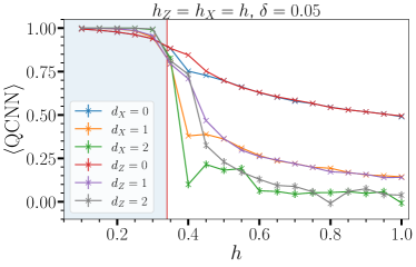
Figure 10: QCNN output for the multicritical point along $h_{X}=h_{Z}$. In comparison to Figure 4 b) in the main text, we plot each pooling layer individually instead of taking the product over the pooling in both bases. We observe a splitting in the values of corresponding $d_{X}$ and $d_{Z}$. This results from the property that the ground state of the Toric Code manifold in this case is two-fold degenerate with a respective bias towards one type of stabilizer. If we initialize the MPS with $\delta=-0.05$, the behavior of both pooling bases will interchange.

As we discussed in the previous section, the QCNN can be entirely run as a quantum circuit but has the benefit that it can also be fully realized in classical post-processing. We sample spin configurations in the Z-basis and in the X-basis from the ground states. We determine the QCNN output in classical post-processing as explained in the previous section. For our simulations, we draw samples for a total of 486 qubits on a $2l_{1}l_{2}=2\times 27\times 9$ qubit lattice. A reduced schematic of the lattice can be found in Figure 11. In the lattice dimensions, the factor of two refers to the two shifted sublattices for qubits either on horizontal or vertical lattice edges. Furthermore, $l_{1}$ is the number of qubits in the horizontal dimension and $l_{2}$ in the vertical direction.

We chose these specific dimensions $l_{1}$ and $l_{2}$ such that we can apply two consecutive pooling layers, which fixes the vertical (periodic) dimension to $l_{2}=9$ qubits. Intuitively, the same minimum number of qubits should also suffice for the QCNN in horizontal dimension, but as the MPS is non-periodic in this direction, we have to use additional qubits as a buffer. This is necessary because the open boundaries break the properties of the convolution $U_{C}^{(0)}$ at the edges. We solve this problem by first applying the QCNN to all sampled qubits, but only extracting information from the qubits, for which the light cone is restricted to the bulk of the lattice and does not span out to the edges as sketched in Figure 11. This requirement must be respected in every layer of the QCNN. Hence, we can find a lower limit for the required number of qubits by defining the lattice configuration for the highest layer. From the QCNN structure, we know that the number of qubits increases by a factor of 9 for every pooling layer and the highest output layer consists of a column of two qubits. To mitigate the edge interactions on the non-periodic dimension of the cylinder code, we need to trim at least one column of qubits on each side of the contributing qubits in horizontal dimension. Accordingly, the output layer must be grown to a number of $N=3\times 2$ qubits to the triple of the original size in dimension $l_{1}$. As all qubits in the higher layers must be propagated from lower layers, the lower layers must all also be tripled in horizontal dimension to a final size of $l_{1}=27$, but all target qubits but the left- and rightmost column can contribute to the results.

[width=0.45]standalone/MPS_snake [width=0.45]standalone/QCNN_cone4

Figure 11: a) Structure of the MPS on the cylindric lattice. Using the snake over the lattice we map the system to a one-dimensional MPS. Hereby, qubit interactions span the periodic dimension $l_{2}$, whereas the lattice goes to infinity in the dimension $l_{1}$, forming an infinite cylinder. b) Lattice dimensions for MPS simulations. The green area from top to bottom resembles the light cone of the output qubits. Due to the infinite horizontal dimension, we need to ensure to only evaluate bulk behavior in horizontal direction in order to avoid propagating effects of the wrong boundary conditions to the output qubits. Therefore, we need to triple the horizontal lattice dimension in every layer, such that the edge behavior can be mapped in the highest layer to qubits that do not need to be measured. In the figure, the tripled dimension is shown with the outer dashed lines. In comparison, the inner dashed lines show a minimal example of the light cone of the output qubits. This resembles the minimum reduction factor of qubits that are necessary for one pooling step. To get improved statistics in each layer versus the minimal example we can evaluate all qubits up to the edge in the green region.

In Figure 12 we plot the QCNN output, for the input state being the reference state of the topological phase, over simultaneous Pauli-Z and Pauli-X noise with corresponding error probabilities $p_{Z}$ and $p_{X}$. For this case, we consider up to 4 layers of QCNN pooling (corresponding to around 120,000 qubits). Figure 12 shows that the same output transition can be found for both error bases. Again, the sharpness of the transition increases with additional QCNN layers. Furthermore, the area classified as topological is of square shape, which is due to the symmetry under the basis transformation of the stabilizer mapping in the Toric Code. Accordingly, the corresponding stabilizer syndromes are mapped to the disjunct sublattices and processed separately in the QCNN.

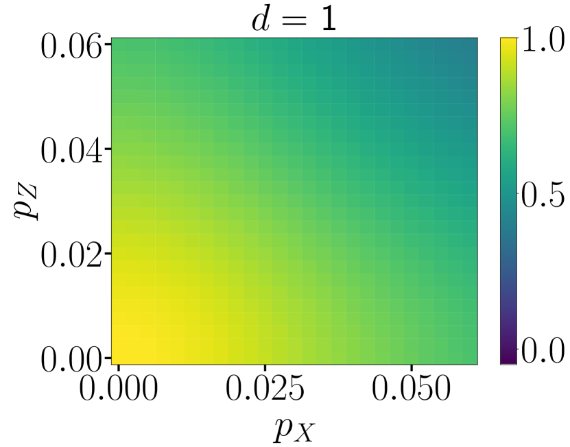
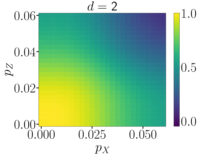
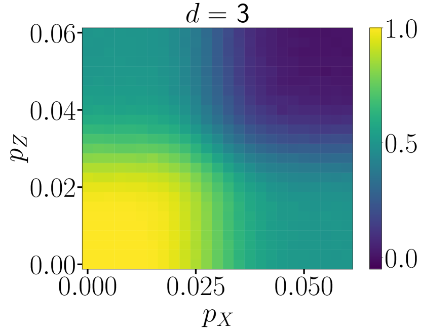
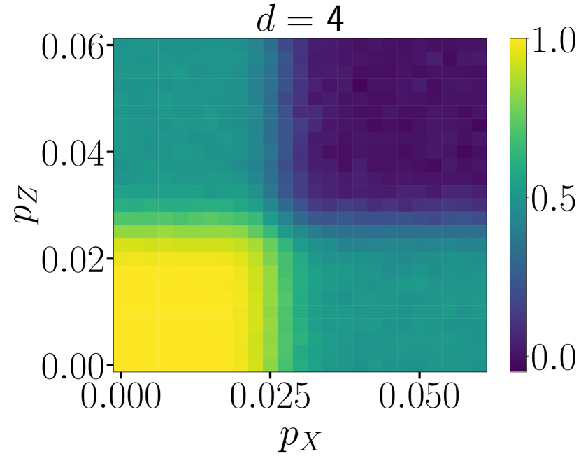
Figure 12: Two-dimensional plots for the QCNN output for simultaneous errors in the X- and Z-basis. We observe increased sharpness for the transition between the topological phase and the disordered regime for error rates higher than $p_{\mathrm{th}}=2.28\%$ with additional pooling layers. These plots show, that the flip errors of the respective basis do not interact with each other during the processing in the QCNN, as is apparent by the square area that is characterized as topological.