Eigenvalue backward errors of Rosenbrock systemsDing Lu, Anshul Prajapati, Punit Sharma, and Shreemayee Bora
Eigenvalue backward errors of Rosenbrock systems and optimization of sums of Rayleigh quotient
Abstract
We address the problem of computing the eigenvalue backward error of the Rosenbrock system matrix under various types of block perturbations. We establish computable formulas for these backward errors using a class of minimization problems involving the Sum of Two generalized Rayleigh Quotients (SRQ2). For computational purposes and analysis, we reformulate such optimization problems as minimization of a rational function over the joint numerical range of three Hermitian matrices. This reformulation eliminates certain local minimizers of the original SRQ2 minimization and allows for convenient visualization of the solution. Furthermore, by exploiting the convexity within the joint numerical range, we derive a characterization of the optimal solution using a Nonlinear Eigenvalue Problem with Eigenvector dependency (NEPv). The NEPv characterization enables a more efficient solution of the SRQ2 minimization compared to traditional optimization techniques. Our numerical experiments demonstrate the benefits and effectiveness of the NEPv approach for SRQ2 minimization in computing eigenvalue backward errors of Rosenbrock systems.
keywords:
Rosenbrock system matrix, eigenvalue backward error, joint numerical range, generalized Rayleigh quotient, nonlinear eigenvalue problem15A18, 15A22, 65K05
1 Introduction
Consider the Rosenbrock system matrix (also known as the Rosenbrock system polynomial) in the standard form [6, 18, 27]:
| (1.1) |
where , , , is an identity matrix of size , and is a matrix polynomial of degree given by with for . A scalar is called an eigenvalue of if .
The Rosenbrock system matrix (1.1) and its associated eigenvalues are of fundamental importance in the field of linear system theory. It is well-known that the dynamical behaviour of a linear time-invariant system in the form of
| (1.2) |
can be analyzed through the system matrix in (1.1), as it contains the information on the poles and zeros of the transfer function of , which determine the stability and performance of the system. The eigenvalues of are known as the invariant zeros of and can be used to recover the zeros of the system. For more details, refer to [27].
The Rosenbrock system matrix is also found in solving rational eigenvalue problems, where for a given a rational matrix function , we seek scalars such that . Rational eigenvalue problems constitute an important class of nonlinear eigenvalue problems with numerous applications, including vibration analysis and solution of (genuine) nonlinear eigenvalue problems; see, e.g., [11, 19, 22, 31]. A popular method for solving rational eigenvalue problems is the linearization of through its state-space realization, expressed as
| (1.3) |
where , and is matrix polynomial of degree and size . This rational linearization technique was introduced by [29] and further developed in [6, 7, 15, 16, 17, 18]. The construction and analysis of the linearization rely on the fact that, under mild assumptions, the eigenvalues of given by (1.3) can be recovered from the eigenvalues of the Rosenbrock system matrix (1.1).
The main purpose of this paper is to perform an eigenvalue backward error analysis for the Rosenbrock system matrix (1.1), taking into account both full and partial perturbations across its four component blocks: , , , and . The eigenvalue backward error is a fundamental tool in both the theoretical study and practical application of numerical eigenvalue problems [28]. As a metric for the accuracy of approximate eigenvalues, backward error is commonly applied in the stability analysis of eigensolvers. Moreover, the backward perturbation matrix can also provide useful insights into the sensitivity of eigenvalues to perturbation in the coefficient matrices.
The eigenvalue backward error for matrix polynomials have been extensively studied in the literature; see, e.g., [2, 3, 4, 12, 13, 25, 30]. A recurring theme in those studies is the preservation of particular structure within the perturbation matrices, such as symmetry, skew-symmetry, and sparsity. However, these works have not yet explored the unique block structure in the Rosenbrock system matrix given by (1.1), despite the prevalence of such matrix polynomials.
Preserving the block structures within for backward error analysis holds practical significance. For instance, in the linear system (1.2), certain coefficient matrices may be exempt from perturbation due to system configurations, and a block-structured perturbation to the Rosenbrock system can best reflect such constraints. For rational eigenvalue problems with given by (1.3), maintaining the block structure in the perturbation matrix to allows for the derivation of eigenvalue backward errors relating to the coefficient matrices of the rational matrix function , by exploiting equivalency of the two eigenvalue problems. Currently, there is limited research on backward error analysis for rational eigenvalue problems. Notably, [5] discusses backward errors for eigenpairs, and a recent study [26] addresses backward errors in the context of perturbation matrix structures, such as symmetric, Hermitian, alternating, and palindromic.
1.1 Contribution and outline of the paper
The main contribution of the paper is two-fold: (i) to establish computable formulas for the eigenvalue backward errors of the Rosenbrock system matrix under various types of perturbations to the blocks , and in , and (ii) to develop a novel approach based on nonlinear eigenvector problems for the solution of related optimization problems.
The rest of the paper is organized as follows. In Section 2, we introduce the backward errors for an approximate eigenvalue of a Rosenbrock system matrix given by (1.1). We consider various types of perturbations to the blocks , and of , including fully perturbing all four blocks and partially perturbing only one, two, or three of these blocks. We show that the computation of those backward errors will lead to a particular type of minimization problem over the unit sphere, where the objective function is the Sum of Two generalized Rayleigh Quotients (SRQ2) of Hermitian matrices. Note that optimization problems involving Rayleigh quotients are commonly employed for structured backward error analysis of eigenvalue problems, see, e.g., [12, 13, 21, 25].
In Section 3, we focus on the SRQ2 minimization problem. Our development is based on the observation that such problems can be reformulated as minimization problems over the joint numerical range (JNR) of three Hermitian matrices. This allows us to exploit the inherent convexity in the JNR for the solution of the problem. Particularly, we establish optimality condition in the form of Nonlinear Eigenvalue Problem with eigenvector dependency (NEPv). This leads to a more efficient and reliable solution of SRQ2 minimization. Moreover, the convex JNR also allows for convenient visualization of the optimal solution and verification of global optimality.
In Section 4, we present numerical examples of SRQ2 minimization, intended for computing eigenvalue backward errors of the Rosenbrock system matrix, and demonstrate the performance of NEPv approach compared to the state-of-the-art optimization technique for SRQ2 minimization. We conclude in Section 5.
1.2 Notations
(or ) is the set of complex (or real) matrices, with (or ). is the identity matrix. For a vector or matrix , is the transpose, is the conjugate transpose, is the -norm (i.e, spectral norm), and is the Frobenius norm. We use
to denote a unit sphere in the -norm in . For a Hermitian matrix , (or ) means that it is positive semidefinite (or definite). We use to denote the smallest eigenvalue of a Hermitian matrix , and to denote the smallest eigenvalue of a definite Hermitian matrix pencil . We will use frequently generalized Rayleigh quotients , with , for positive semidefinite and , where we assume that
| (1.4) |
By the definition (1.4), the function is well-defined and lower semi-continuous, i.e., , for all , so we can properly define optimization problems involving Rayleigh quotients in later discussions. Since Rayleigh quotients are homogeneous, i.e., for , we can restrict its variable to .
2 Backward Error Analysis of Rosenbrock Systems
We consider eigenvalue backward error of the Rosenbrock system matrix (1.1) subject to various types of block perturbation in its coefficient matrices. The following result is well established in matrix analysis and will be frequently used in our derivation of computable formulas for the backward errors.
Lemma 2.1.
Let , , , and .
-
(a)
If , then and the minimizer .
-
(b)
If and , then and the minimizer .
-
(c)
If and , then and has no solution.
Proof 2.2.
It follows from standard analyses in optimization that the minimizer is unique, as the objective function is strongly convex and is a convex set; see, e.g., [24]. For all , the constraint leads to . For item (a) with , we have , where the equality holds for , which satisfies . Items (b) and (c) follow from straightforward verification.
2.1 Backward Error with Full Perturbation
Let be a perturbation to the Rosenbrock system matrix in the form of
| (2.1) |
where , and , with for , representing perturbations to the corresponding coefficient matrices of the Rosenbrock system in (1.1). The magnitude of the perturbation is naturally measured by the Frobenius norms of its coefficient matrices, i.e.,
| (2.2) |
We introduce the following notion of eigenvalue backward error of Rosenbrock systems.
Definition 2.3.
Remark 2.4.
First, if is an eigenvalue of , then the backward error vanishes, since is a solution to (2.4). Second, for all , we have bounded by , by taking the feasible perturbation in (2.4). Moreover, the minimal perturbation in (2.4) is always achievable, i.e., there exists such that . This is because is a polynomial in the coefficients of . The set of feasible perturbations of (2.4), which is the zero set of the polynomial as given by , must be a closed set. Consequently, in the minimization (2.4), the continuous objective function over a closed set of can always achieve its minimal value.
Working directly with the constraint on the determinant of a matrix, as in the formula for backward error in (2.4), may pose computational challenges. Instead, we can use the fact that a square matrix has if and only if for some nonzero vector . We can hence reformulate the optimization problem (2.4) as
| (2.5) |
where the second equation separates the variables and into a bi-level optimization. For the inner minimization problem on , we can show that the minimal value can be expressed as the sum of two generalized Rayleigh quotients (SRQ2) in . Consequently, we obtain a characterization of through an SRQ2 minimization problem, as shown in the following result.
Theorem 2.5.
Proof 2.6.
Consider the inner minimization problem of (2.5):
| (2.8) |
where is a fixed vector. By the block form of coefficient matrices in (2.1),
| (2.9) |
and we can also write the constraint on equivalently to
| (2.10) |
Here, the second equation is further equivalent to
| (2.11) |
and we have partitioned with and .
We can minimize the two components of in (2.9) separately. First, by Lemma 2.1, among all perturbation satisfying the first equation of (2.10),
| (2.12) |
achieves the minimal Frobenius norm, which is given by
| (2.13) |
where is given by (2.7). Similarly, among all perturbation satisfying (2.11), the following matrix achieves the minimal Frobenius norm
| (2.14) |
where , with the Frobenius norm satisfying
| (2.15) |
where and are as defined in (2.7), and we used .
From the proof of Theorem 2.5, we can also see that the optimal perturbation achieving the backward error in (2.4) can be generated by the perturbation matrices (2.12) and (2.14) with being a minimizer of the SRQ2 minimization (2.6).
2.2 Backward Error with Partial Perturbations
By partial perturbations, we refer to the cases where only some particular blocks within are perturbed. Let be a subset indicating the names of blocks to be perturbed. A structured perturbation of corresponding to is denoted by
| (2.16) |
where , , , and are as from in (2.1), and is an indicator function, i.e., if , and if . Similar to Definition 2.3, we define the backward error for with a partial perturbation as follows.
Definition 2.7.
Let indicate the names of the blocks to be perturbed. The backward error of an approximate eigenvalue of the Rosenbrock system matrix as in (1.1), subject to the perturbation from the set
| (2.17) |
is defined as
| (2.18) |
where we set , if the constrained optimization problem is infeasible, i.e., there is no perturbation within that satisfies .
Remark 2.8.
Due to the constraint on block structures of perturbation as in (2.16), the optimization problem (2.18) may be infeasible. In such a case, the backward error is unbounded. This is in contrast to the case of full perturbation (2.4), where the backward error is always finite. On the other hand, provided that the minimization (2.18) is feasible, the minimal perturbation in (2.18) can always be attained, as can be justified by using the same arguments as in Remark 2.4.
Similar to (2.5), it is straightforward to write the optimization problem (2.18) as
| (2.19) |
We can then turn it into a bi-level optimization problem, by first fixing and minimizing over , as given by
| (2.20) |
where denotes the solution of the inner optimization problem, i.e.,
| (2.21) |
and we assign if the minimization problem is infeasible.
Like the case of full perturbation in (2.4), we can show that the solution of the minimization problem (2.21) still admits an expression as the sum of (at most) two generalized Rayleigh quotients in . However, the derivation of those solutions will depend on the particular block structure specified in . For analyses, we will categorise the perturbations into three classes, based on the number of blocks in . They are (i) perturbing one single block from , and of , (ii) perturbing any two blocks, and (iii) perturbing any three blocks.
2.2.1 Perturbing a Single Block
Consider the backward error of with only one of the blocks from , , , and to be perturbed. Specifically, we refer to as defined by (2.18) with , for . It will be sufficient to focus on the cases of , , and . Due to symmetry, the backward error can be derived by the formula of applied to the transposed system ; see Remark 2.13.
We begin with a general-purpose lemma on partial perturbations involving a single block before presenting the main result.
Lemma 2.9.
Proof 2.10.
For item (a), we first reformulate the equality constraints in (2.22) as
| (2.25) |
For feasibility, we will need . This condition also implies that , because (recall that is non-singular and ). Since the first equation in (2.25) has a non-zero right hand side, by Lemma 2.1, there exist solution if and only if . This proves the conditions in (2.3).
Theorem 2.11.
Let be a Rosenbrock system matrix given by (1.1), be a scalar with , be Hermitian matrices from (2.7), and and form orthonormal basis of the null spaces of and , respectively. Then, it holds that and , and we have the following characterizations for the eigenvalue backward errors.
-
(a)
if and only if ; Otherwise,
(2.26) -
(b)
if and only if ; Otherwise,
(2.27) -
(c)
if and only if ; Otherwise, with ,
(2.28)
Proof 2.12.
To begin with, we have , due to . Then a quick verification shows and .
For item (a), it follows from (2.20) with that
| (2.29) |
By Lemma 2.9, with and , the inner optimization above has solution
| (2.30) |
where and are as defined in (2.7), and we assumed satisfies
| (2.31) |
as according to the feasibility condition (2.1) (otherwise ). The second constraint, , implies we can parameterize as
| (2.32) |
where is a basis matrix of the null space of (and of (2.7) as well). Consequently, plugging (2.32) into (2.30), and further into (2.29), we obtain
where is due to from (2.31). Clearly, this optimization is feasible if and only if . We thus proved the first equality in (2.26), upon noticing that the Rayleigh quotient yields for satisfying , because of . The second equality is by the well-known minimization principle of Hermitian eigenvalue problems; see, e.g., [28, Chap. VI].
Remark 2.13.
To obtain the backward error of the Rosenbrock system matrix , we can consider the transposed system matrix , as denoted by
| (2.33) |
Then perturbing the block of by is the same as perturbing the block of by . Since , we have , where is the eigenvalue backward error of the new system subject to a perturbation to its block. Here, we can evaluate through Theorem 2.11 (b) applied to .
2.2.2 Perturbing Any Two Blocks
We now consider the cases where exactly two blocks of are to be perturbed, i.e., with . We have six such cases in total, and it is sufficient to focus on the four cases with , , , and . The other two, with and , can be addressed using symmetry by considering the transposed system , as similar to Remark 2.13. Again, we start by discussing a general-purpose lemma before establishing the formulas for the backward errors.
Lemma 2.14.
Let , , and , for , where . Suppose that .
-
(a)
The minimization problem
(2.34) s.t. , , for , is feasible if and only if , where the minimal objective value
(2.35) - (b)
Proof 2.15.
For item (a), we can reformulate the constraints for ’s in (2.34) as
| (2.38) |
In the first equation, because of (due to ), there always exists a solution according to Lemma 2.1. Moreover, the solution with the minimal Frobenius norm satisfies
This leads to the optimal objective value (2.35) for the optimization (2.34), provided that , which ensures the second constraint in (2.38) is also feasible.
For item (b), we can reformulate the constraints for ’s in (2.36) as
| (2.39) |
We can consider the optimal and separately.
For the first equation in (2.39), we derive from Lemma 2.1 that: (i) If , then the solution with the minimal Frobenius norm satisfies
| (2.40) |
(ii) If and , then the solution with the minimal Frobenius norm is , which also satisfies (2.40) by letting the fraction to have value ; and (iii) If and , then there is no solution and the optimization (2.36) is infeasible.
For the second equation in (2.39), we derive from Lemma 2.1 that: (i) If , then the solution with a minimal Frobenius norm satisfies
| (2.41) |
(ii) If and , then the solution with the minimal Frobenius norm is , which satisfies (2.40) by letting the fraction to have value ; and (iii) If and , then there is no solution and the optimization (2.36) is infeasible.
Theorem 2.16.
Let be a Rosenbrock system given by (1.1), be a scalar with , be Hermitian matrices from (2.7), and and form orthonormal basis of the null spaces of and , respectively.
-
(a)
and it satisfies
(2.42) -
(b)
and it satisfies
(2.43) -
(c)
and it satisfies
(2.44) - (d)
Proof 2.17.
For item (a), it follows from (2.21) with that
According to Lemma 2.14 (a) with and , the optimal objective value if and only if (i.e., ), where
By (2.20) and the parameterization of the null vector of , we obtain (2.42).
For item (b), it follows from (2.21) with that
According to Lemma 2.14 (b) with and , the optimal objective value
which leads to (2.43) by recalling (2.20). By taking a particular satisfying and , we can derive from (2.43) that .
Remark 2.18.
To obtain the backward error and of the Rosenbrock system matrix , we can again consider the transposed Rosenbrock system matrix as given by (2.33). By block symmetry in transposing, we have
| (2.46) |
where denotes the eigenvalue backward error of the new system matrix subject to a perturbation pattern . Now, for the perturbation patterns and under consideration, their corresponding backward error can be obtained quickly by the formulas (2.42) and (2.45) applied to the transposed system matrix.
2.2.3 Perturbing Any Three Blocks
Finally, we consider the cases where exactly three blocks of are to be perturbed. There are four such type of perturbations, and we focus on the three cases with , , and . The other case with is readily solved by the transposed system matrix.
Lemma 2.19.
Let , , and , for , where . Suppose that . The minimization problem
| (2.47) | ||||
| s.t. | , , for , | |||
| , for , | ||||
has an optimal objective value given by
| (2.48) |
where for , and we assign a value of to a fraction in the form of . The optimal objective value (2.48) is , if and only if and , indicating the optimization (2.47) is infeasible.
Proof 2.20.
We write the constraints for ’s in (2.47) equivalently to
| (2.49) |
In the first equation, because of (due to ), by Lemma 2.1 there always exists solution and the solution with the minimal Frobenius norm satisfies
| (2.50) |
In the second equation of (2.49), we can derive from Lemma 2.1 that: (i) If , then the solution with the minimal Frobenius norm satisfies
| (2.51) |
(ii) If and , then the solution with the minimal Frobenius norm is , which also satisfies (2.51) by letting the fraction to have a value ; and (iii) If and , then there is no solution and the optimization (2.47) is infeasible.
Theorem 2.21.
Let be a Rosenbrock system matrix as given by (1.1), be a scalar with , and be Hermitian matrices from (2.7).
-
(a)
and it satisfies
(2.52) -
(b)
and it satisfies
(2.53) -
(c)
and it satisfies
(2.54) where .
Proof 2.22.
For item (a), it follows from (2.21) with that
According to Lemma 2.19, with , , and , we obtain
which leads to (2.52) by recalling (2.20). Moreover, by an with , we obtain ,
For item (b), it follows from (2.21) with that
where the equality constraint is obtained from , by switching the column blocks of the matrix . Then, by applying Lemma 2.19 with , , , , the rest of the proof follows that of item (a).
For item (c), it follows from (2.21) with that
where the equality constraint is obtained from , by switching both the row and column blocks of the matrix . Again, by applying Lemma 2.19 with , , , , the rest of the proof follows that of item (a).
Remark 2.23.
The backward error of the Rosenbrock system matrix , can be obtained from the transposed Rosenbrock system matrix as given by (2.33). By block symmetry, we have
| (2.55) |
where denotes the eigenvalue backward error of the new Rosenbrock system matrix subject to a perturbation pattern . Now, can be evaluated by the formula (2.53) applied to the transposed system .
3 Minimization of Sum of Two Rayleigh Quotients
Regardless of full and partial block perturbations, the eigenvalue backward errors of the Rosenbrock system matrix can be expressed as an optimization problem in the form of
| (3.1) |
where are Hermitian and positive semidefinte matrices, are given scalars satisfying , for . For example, in the case of full perturbation with given by (2.3), we can set , , , , , and , noticing that . For partial perturbations, a few cases (Theorems 2.11 and 2.16) involve a single Rayleigh quotient in (i.e., ), but in general we must address two non-trivial Rayleigh quotients.
Since the objective function is the Sum of Two generalized Rayleigh Quotients, we call (3.1) an SRQ2 minimization. Recall that a Rayleigh quotient of the form is assigned a value of by convention (1.4). This ensures in (3.1) is lower semi-continuous (i.e., for ) and hence, the minimization (3.1) is well-defined. Clearly, the objective function is differentiable at satisfying , for (i.e., both denominators of are nonzero).
The SRQ2 minimization (3.1), subject to the spherical constraint , can be solved by conventional Riemannian optimization techniques, such as the Riemannian trust-regions method; see, e.g., [1]. However, those general-purpose Riemannian optimization methods often target local minimizers, and they do not fully exploit the special SRQ2 form of the objective function for analysis and computation.
In this section, we introduce a novel technique to solve the SRQ2 minimization (3.1). We will recast the problem into an optimization over the joint numerical range of the Hermitian matrices . The new problem typically presents fewer local minimizers than the original one, so it is more favorable for analysis and computation. The convexity in the joint numerical range also allows for development of a nonlinear eigenvector approach to efficiently solve the optimization problem, as well as a visualization technique to aid in verification of the global optimality of solution.
3.1 Minimization Over Joint Numerical Range
Let contain the coefficient matrices of the SRQ2 minimization (3.1). We define the Joint Numerical Range (JNR) associated with as
| (3.2) |
where consists of the quadratic forms of the Hermitian matrices in :
| (3.3) |
It is well-known that the JNR is a closed and connected region in , and it is a convex set if the size of the matrices satisfies ; see, e.g., [8, 23].
In the SRQ2 minimization (3.1), the objective function is defined through the three quadratic forms , for . Hence, we can write
| (3.4) |
where is given by
| (3.5) |
and . Consequently, by using an intermediate variable , we recast the SRQ2 minimization (3.1) into
| (3.6) |
where the feasible set , the JNR as defined in (3.2), contains all possible values of over . We call problem (3.6) the JNR minimization associated with the SRQ2 minimization (3.1).
In the JNR minimization (3.6), the variable is a real and -dimensional vector, as in contrast to a complex and -dimensional variable vector of the original SRQ2 minimization (3.1). Typically, in practice, so the new feasible region for is a convex set. This convexity facilitates analysis, computation, and visualization the JNR minimization (3.2), as to be shown shortly.
Since the map is generally not bijective, the two optimization problems (3.1) and (3.6) are, however, not strictly equivalent. The relationship of the solution for the two problems are summarized in Lemma 3.1. Recall that by the standard notion in optimization, a general optimization problem has a global minimizer , if it holds for all . It has a local minimizer , if for all with sufficiently close to .
Proof 3.2.
We stress that the reverse of Lemma 3.1 (b) is not necessarily true. Namely, if is a local minimizer of the SRQ2 minimization (3.1), then may not be a local minimizer of the JNR minimization (3.6). This implies the JNR minimization (3.6) may have much fewer local minimizers than the original SRQ2 minimization (3.1). This is a desirable property, since the local optimization technique will have a better chance to find the global optimal solution.
3.2 Local Optimality Condition and NEPv
By exploiting the convexity in the JNR, we will establish a variational characterization for the local minimizers of the JNR minimization (3.6). This characterization can also be equivalently expressed as a nonlinear eigenvalue problem with eigenvector dependency (NEPv).
Theorem 3.3.
Let , for , be Hermitian matrices of size , , be as defined in (3.2), and be as given by (3.5). Suppose that is a local minimizer of in , and is differentiable at , then
| (3.7) |
Moreover, (3.7) holds if and only if for an satisfying the NEPv:
| (3.8) |
where is a Hermitian matrix given by
| (3.9) |
and is the smallest eigenvalue of .
Proof 3.4.
We first show equation (3.7). Let be an arbitrary point in . Recall that the JNR is a convex set for matrices of size (see, e.g., [8]). By convexity, contains the entire line segment between and . Namely,
| for all . |
Since is differentiable at , by Taylor’s expansion of at ,
The local minimality of implies for sufficiently small, so it holds that , i.e.,
Since the inequality above holds for all , we can derive
where the last inequality is by . As equality must hold, we obtain (3.7).
Next we show for some satisfying the NEPv (3.8). Since and , we can write and for some , according to the definition in (3.2). We can derive
| (3.10) |
where in the last equality we used the gradient of the function defined in (3.5):
Using (3.10), we can write the characterization (3.7) as
According to the well-known minimization principle of the Hermitian eigenvalue problems, the minimal value of the quadratic form from above is achieved at the eigenvector of the smallest eigenvalue of . Consequently, is the eigenvector for the smallest eigenvalue of the Hermitian matrix . We proved (3.8).
By Theorem 3.3, the NEPv (3.8) and the equivalent variational equation (3.7) provide local optimality condition for the JNR minimization (3.6). We note that those conditions are stronger than the standard first-order optimality condition for the original SRQ2 minimization (3.1), for which, by introducing the Lagrange function and set (assuming is a real vector so that is differentiable), we obtain the same equation as (3.8) but do not require to be the smallest eigenvalue of . This advantage of NEPv characterization is partially explained by the relation of the two optimization problems revealed in Lemma 3.1.
In the literature, NEPv characterizations have been explored in various optimization problems with orthogonality constraints; see [10] and references therein. Those characterizations allow for efficient solution of the optimization problem by exploiting state-of-the-art eigensolvers. Particularly, in [33, 35] the authors proposed NEPv characterizations that apply to the optimization of sum of Rayleigh quotients:
| (3.11) |
where for are Hermitian positive definite matrices*** The works [33, 35] focus on maximization of rather than minimization, and they assume . These problems are equivalent to (3.11) by negating and shifting the objective function to , with . Additionally, they only consider real and . However, we can always represent the variable by its real and imaginary parts as , thereby converting (3.11) into an equivalent real form. . Our development of the NEPv differs from the previous works [33, 35] in several aspects. First, the SRQ2 minimization (3.1) cannot generally be reduced to the form of (3.11), due to the presence of semidefinite matrices in both denominators of the objective function in (3.11). Therefore, the previous analyses [33, 35] do not directly apply to the SRQ2 minimization (3.1). Second, the developments in [33, 35] primarily rely on the KKT conditions and properties of the global optimal solution of the optimization problem (3.11). In contrast, by exploiting the JNR minimization (3.6), our Theorem 3.3 reveals the nature of NEPv (3.8) as the first-order local optimality condition of the JNR minimization (3.6). Combined with Lemma 2.1, this insight explains why NEPv (3.8) can characterize global optimality but not local optimality of the minimization problem (3.11), advancing the previous observations in [33, 35]. Additionally, our use of the JNR significantly simplifies the derivation of NEPv for (3.11). Particularly, by a straightforward extension, it provides a unified treatment for problem (3.11) and its block extension given by: Minimize subject to and . Similar trace minimizations were considered in [35], but over the real Stiefel manifold with variables and .
3.3 Non-differentiable Minimizers
Theorem 3.3 requires the local minimizer to be differentiable for the rational function , but this is not a significant restriction. The non-differentiability issue can occur if one of the fractions in , as given by (3.5), takes the form . We will show that such non-differentiable local minimizers can be quickly identified by Hermitian eigenvalue problems.
For simplicity, we assume the two positive semidefinite matrices in the denominators of the objective function of the SRQ2 minimization (3.1), for , do not share any common null vectors. Equivalently, this is expressed as
| (3.12) |
given that . The condition (3.12) holds for all SRQ2 minimizations from the backward error analysis of Rosenbrock systems discussed in Section 2. Moreover, to determine the differentiability of , we introduce the Hermitian matrices
| (3.13) |
corresponding to each Rayleigh quotient in the function given by (3.1). Recalling that and , we have . A quick verification shows that if and only if the Rayleigh quotient won’t encounter the form .
Theorem 3.5.
Let assumption (3.12) hold for the JNR minimization (3.6) and be given by (3.13). Let be a local minimizer of over with .
-
(a)
If and , then must be a differentiable point for , and hence, it admits the NEPv characterization given by Theorem 3.3.
-
(b)
Otherwise, may be non-differentiable for , and then it must be given by for or , where is an orthogonal basis matrix of the null space of , and denotes an eigenvector for the smallest eigenvalue of the following Hermitian eigenvalue problems:
(3.14a) (3.14b) where the two Hermitian matrices on the right-hand side are positive definite.
Proof 3.6.
By (3.5), we can write the objective function as with
| (3.15) |
for , where we parameterize by an . Clearly, is differentiable at if and only if the denominator
For item (a), by parameterizing , we must have for . Because otherwise, we have . Then by (3.15), , contradicting . Hence, is differentiable at .
For item (b), suppose that is not differentiable at , i.e., its denominator in definition (3.15) vanishes: . Since , the numerator in must also vanish: . So, we have
| (3.16) |
where we used and and is an orthogonal basis matrix.
Now, by the local minimality of and Lemma 3.1, we have must be a local minimizer of with restricted to the subspace :
| (3.17) |
where the first equality is due to and for all (recalling (3.16) and our convention (1.4)). Moreover, since the assumption (3.12) implies that for do not have a common null vector, we have for the matrix in the denominator of (3.17).
As a well established result in matrix analysis and optimization, a local minimizer of a Rayleigh quotient must be its global minimizer; see, e.g., [1, Prop 4.6.2]. By (3.17) and Hermitian eigenvalue minimization principle, , where is the eigenvector for the smallest eigenvalue of the Hermitian eigenvalue problem (3.14a).
Analogously, if is not differentiable at , then we have , where is an eigenvector for the smallest eigenvalue of the eigenvalue problem (3.14b).
In certain cases of partial block perturbations, as described in Theorems 2.16 and 2.21, the corresponding SRQ2 minimization may not have positive definite or matrices. To find the minimal solution of these problems, we can solve NEPv (3.8), provided it has a solution, along with the Hermitian eigenvalue problems (3.14). We can then select the with the minimal object value as the solution.
4 Numerical Experiments
We present numerical examples of SRQ2 minimization (3.1) for backward error analysis of the Rosenbrock system matrix. Our primary goal is to demonstrate the benefits of the JNR reformulation (3.6), including elimination of certain local minimizers of (3.1), efficient solution via the NEPv characterization (3.8), and visualization of the solution. All experiments are implemented in MATLAB and run on a MacBook Pro laptop with an M1 Pro CPU and 32G memory. Codes and data are available through https://github.com/ddinglu/minsrq2.
To solve NEPv (3.8), we apply the level-shifted Self-Consistent-Field (SCF) iteration [10, 32, 34]: Starting from an initial guess , iteratively solve Hermitian eigenvalue problems
| (4.1) |
for , where is a given level-shift, and is the eigenvector corresponding to the smallest eigenvalue of the Hermitian matrix . If , then (4.1) reduces to the plain SCF iteration. But a non-zero level-shift can help to stabilize and accelerate the convergence of plain SCF. Particularly, a plain SCF may not always converge, whereas for sufficiently large , level-shifted SCF is guaranteed locally convergent under mild assumptions; see, e.g., [10]. In our implementation, we select level-shifts adaptively by sequentially trying
| (4.2) |
until a reduction in the objective function or residual norm of NEPv is achieved by . Here, is the eigenvalue gap between the first and second smallest eigenvalue of , and the use of is a common practice; see, e.g., [32, 34]. Often, a plain SCF () can produce a reduced , and then there is no need to enter the selection loop (4.2) for . Finally, the level-shifted SCF (4.2) is considered to have converged if the relative residual norm satisfies
| (4.3) |
and denotes the matrix 1-norm (i.e., maximal absolute column sum). We mention that the performance of SCF can be further enhanced by various acceleration techniques, such as damping, Anderson acceleration, preconditioning, etc; see, e.g., [9] and references therein. But those techniques are beyond the scope of this paper.
To solve SRQ2 minimization (3.1) directly, we apply the Riemannian Trust-Region (RTR) method [1] – a state-of-the-art algorithm for optimization problems with orthogonality constraints and available in the software package MANOPT [14]. The stopping criteria of RTR is based on the norm of the Riemannian gradient, which coincides with twice the residual norm with ; see, e.g., [1]. For consistency with (4.3) in algorithm comparison, the error tolerance of RTR will be set as twice the residual norm of the last iteration by level-shifted SCF.
For demonstration, we compute the convex JNR by sampling its boundary points. A boundary point of with a given outer normal direction is computed by , where the eigenvector for the smallest eigenvalue of Hermitian eigenvalue problem
| (4.4) |
We refer to [10, 20] for details on the computation of JNR. To show a number is the global minimal value of over , we can check visually if the entire JNR would lie on one side of the level surface .
Example 4.1.
This example is to show that the JNR minimization (3.6) can avoid certain local minimizers of the original SRQ2 minimization (3.1). To demonstrate, we consider an SRQ2 minimization of size in the following form
| (4.5) |
where the coefficient matrices are randomly generated and given by
and . Solving SRQ2 minimization (4.5) by the Riemannian trust-region method with various starting vectors, we found two optimal solutions
| (4.6) |
Both are local minimizers of SRQ2 minimization (4.5), since the Hessian matrices for at can be verified positive definite over the complement of – a sufficient condition for local optimality of the constrained minimization (4.5); see, e.g., [24, 33].
By a change of variable , the SRQ2 minimization (4.5) can be written as the following JNR minimization problem
| (4.7) |
where . Here, we recall (3.2) for the definition of the joint numerical range . The local minimizers from (4.6) yield as given by
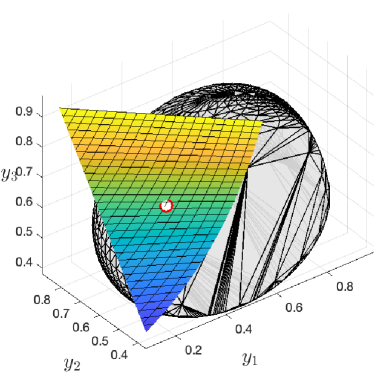
| (4.8) |
Those optimal solutions are depicted in Figure 4.1, thanks to that the JNR minimization (4.7) is over , which allows for convenient visualization. The joint numerical range lies on one side of the level surface , indicating is (at least) a local minimizer of JNR minimization (4.7). Whereas the level surface cuts through , implying is not a local minimizer. That is to say, despite both and are local minimizers of SRQ2 minimization (4.5), only occurs as a local minimizer of JNR minimization (4.7).
By Theorem 3.3, since is a local minimizer of JNR minimization (4.7), the corresponding must be a solution to the NEPv (3.8). Numerically,
where is the smallest eigenvalue of , indicating is an approximate eigenvector of NEPv (3.8). In contrast, we have for the other solution that
indicating is not an eigenvector of NEPv (3.8). This is consistent to the fact that is not a local minimizer of the JNR minimization (4.7). Indeed, we have ; i.e., is with the second smallest eigenvalue of , rather than the smallest one as required by NEPv (3.8). Hence, solving NEPv (3.8) can avoid the local minimizer of SRQ2 minimization (4.5).
Finally, it can be verified that the approximate joint numerical range in Figure 4.1 lies entirely on one side of the level surface, justifying pictorially that the solution is a global minimizer of (4.7). Here, the approximate is constructed by the convex hull of sampled boundary points of with uniformly distributed normal directions. Each boundary point is computed by solving a Hermitian eigenvalue problems of size as given by (4.4). See [10] for details of the computation.
Example 4.2.
For some specialized SRQ2 minimization in the form of (3.11), it is known that NEPv characterization, as the one given by (3.8), allows for the use of state-of-the-art eigensolvers for fast solution of the problem; see, e.g., [33, 34]. In this example, we consider SRQ2 minimization (3.1) intended for computing eigenvalue backward error of the Rosenbrock systems, and demonstrate the performance of NEPv approaches. For experiment, we consider a Rosenbrock system matrix with a linear , as given by
| (4.9) |
where the coefficient matrices are randomly generated (using the MATLAB code M = randn(m,n)+1i*randn(m,n)) and the dimensions are set to and . We compute the backward error with full perturbation using the formula (2.6). For testing, we generate the approximate eigenvalue by first perturbing the coefficient matrices of (4.9) entrywisely by randn*1.0E-1, and then choosing as an eigenvalue of the perturbed linear system. We thus anticipate the backward error of such to be at the same order of the perturbation .
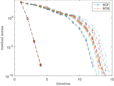
Recall that the formula of the backward error in (2.6) involves an SRQ2 minimization in the form of (3.11) – with coefficient matrices , , and from (2.7). The left panel of Figure 4.2 reports the convergence history of the Riemannian trust-region method for solving this optimization, as well as the level-shifted SCF (4.1) for the corresponding NEPv (3.8). We have repeatedly run the algorithms times with different and randomly generated starting vectors . In all testing cases, SCF rapidly converged in three iterations, despite of a seemingly linear rate of convergence, and the algorithm is insensitive to the choice of initial vectors. In comparison, the RTR requires more iterations – although its local convergence rate seems superlinear, the initial convergence is relatively slow. We note that the total number of iterations by RTR is about times that of SCF, but SCF is about times as fast in computation time:
This indicates the average cost per iteration of RTR is more expensive than that of SCF. The reason is mainly because RTR required a large number of inner iterations to solve the trust-region subproblem at each (outer) iteration [1]. Taking inner iterations into account, RTR requires an average of 176 iterations, and level-shifted SCF still requires (i.e., are always accepted and the process is indeed a plain SCF).
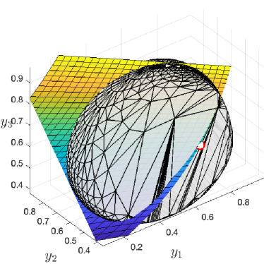
For all the runs with different starting vectors, both RTR and SCF have converged to the same solution, yielding the backward error which is indeed at the same order of the perturbation . The global optimality of the computed solution is verified pictorially in the right panel of Figure 4.2 through the corresponding JNR minimization in the form of (4.7).
Example 4.3.
This example is to demonstrate the computational efficiency of NEPv approaches for various SRQ2 minimization (3.1) from Section 2 for the computation of backward error of Rosenbrock systems with different types of block perturbations. We will focus on types of block perturbation, including ‘AP’, ‘BC’, ‘ABC’, ‘ABP’, ‘ACP’, ‘BCP’, and ‘ABCP’, where the letters indicate the perturbing blocks in the Rosenbrock system matrix (1.1). The formulas of backward error for each of those perturbation type are found in Section 2, and they all involve SRQ2 minimization (3.1). Note that we have discussed a total of cases of partial block perturbations in Section 2, among which cases can be conveniently solved by Hermitian eigenvalue problems and, hence, are not reported in our experiments.
| ‘timing (# iteration)’ per type of block perturbation | ||||||||
| Alg | AP | BC | ABC | ABP | ACP | BCP | ABCP | |
| SCF | 0.4 ( 7) | 1.1 (48) | 0.8 (38) | 0.2 ( 6) | 0.1 ( 5) | 0.1 ( 5) | 0.1 ( 3) | |
| RTR | 4.2 (43) | 3.3 (19) | 3.8 (26) | 1.8 (14) | 6.3 (46) | 1.9 (14) | 1.8 (14) | |
| SCF | 1.7 ( 6) | 1.0 (14) | 1.0 (14) | 0.3 ( 4) | 0.2 ( 3) | 0.5 ( 3) | 0.2 ( 3) | |
| RTR | 22.0 (43) | 10.7 (26) | 10.3 (35) | 5.5 (15) | 18.6 (39) | 7.0 (15) | 33.5 (29) | |
| SCF | 4.9 ( 5) | 2.0 (12) | 2.2 (13) | 0.9 ( 4) | 0.5 ( 3) | 0.5 ( 3) | 0.4 ( 2) | |
| RTR | 52.2 (80) | 38.3 (24) | 29.0 (31) | 24.8 (19) | 88.1 (70) | 28.9 (17) | 25.5 (18) | |
| SCF | 18.7 ( 5) | 4.4 (14) | 4.7 (15) | 1.2 ( 4) | 1.2 ( 3) | 0.9 ( 3) | 0.6 ( 2) | |
| RTR | 177.9 (76) | 61.1 (22) | 63.4 (37) | 44.4 (17) | 118.8 (62) | 52.9 (16) | 43.6 (17) | |
| ‘timing (# iteration)’ per type of block perturbation | ||||||||
| Alg | AP | BC | ABC | ABP | ACP | BCP | ABCP | |
| SCF | 0.9 ( 9) | 0.2 (12) | 0.2 ( 5) | 0.9 ( 8) | 0.1 ( 6) | 0.2 (12) | 0.1 ( 5) | |
| RTR | 3.5 (14) | 2.7 (12) | 1.8 (11) | 2.8 (17) | 2.3 (11) | 2.7 (13) | 1.8 (11) | |
| SCF | 8.5 ( 9) | 0.7 ( 9) | 0.3 ( 4) | 0.6 ( 7) | 0.4 ( 5) | 0.7 ( 9) | 0.3 ( 4) | |
| RTR | 19.5 (21) | 15.9 (14) | 9.1 (12) | 23.5 (25) | 10.9 (12) | 12.9 (13) | 9.2 (12) | |
| SCF | 18.6 ( 8) | 1.3 ( 7) | 0.9 ( 3) | 16.2 ( 7) | 1.2 ( 5) | 1.8 ( 8) | 0.8 ( 4) | |
| RTR | 40.7 (17) | 30.8 (12) | 16.7 (10) | 27.0 (16) | 18.7 (10) | 34.1 (12) | 15.7 (10) | |
| SCF | 41.5 ( 7) | 2.5 ( 8) | 0.9 ( 3) | 31.7 ( 6) | 1.9 ( 4) | 2.8 ( 9) | 1.6 ( 4) | |
| RTR | 77.8 (22) | 59.1 (12) | 36.5 (12) | 57.0 (21) | 33.9 (11) | 68.0 (13) | 35.3 (12) | |
| ‘timing (# iteration)’ per type of block perturbation | ||||||||
| Alg | AP | BC | ABC | ABP | ACP | BCP | ABCP | |
| SCF | 0.8 ( 8) | 0.8 ( 8) | 0.5 ( 7) | 0.5 ( 7) | 0.3 ( 5) | 0.3 ( 5) | 0.2 ( 3) | |
| RTR | 6.1 (14) | 8.2 (14) | 9.4 (15) | 7.3 (15) | 9.1 (15) | 8.5 (14) | 6.0 (14) | |
| SCF | 2.5 ( 8) | 2.5 ( 8) | 2.4 ( 7) | 2.9 ( 7) | 1.6 ( 5) | 1.6 ( 5) | 0.9 ( 3) | |
| RTR | 40.3 (15) | 49.7 (16) | 41.0 (16) | 45.8 (16) | 59.5 (16) | 57.0 (16) | 41.5 (16) | |
| SCF | 7.2 ( 8) | 6.9 ( 8) | 6.3 ( 7) | 6.2 ( 7) | 4.0 ( 5) | 4.0 ( 5) | 3.5 ( 4) | |
| RTR | 182.0 (18) | 167.4 (18) | 167.7 (18) | 136.5 (17) | 224.3 (18) | 131.0 (17) | 130.7 (17) | |
| SCF | 12.8 ( 8) | 14.9 ( 8) | 11.4 ( 7) | 11.2 ( 7) | 8.3 ( 5) | 8.0 ( 5) | 5.6 ( 3) | |
| RTR | 284.4 (16) | 396.5 (20) | 293.8 (18) | 263.9 (17) | 383.5 (17) | 429.5 (19) | 217.8 (16) | |
For experiment, we still use the Rosenbrock system matrix (4.9) from Example 4.2. We generate such with various dimensions and and compute the eigenvalue backward errors for different types of block perturbations via SRQ2 minimization (3.1). It is verified that condition (3.12) holds for all the SRQ2 minimizations, so their optimal solutions are characterized by the NEPv (3.8) due to Theorem 3.5. In the test, we compare the performance of Riemannian trust-region method for directly solving SRQ2 minimization (3.1) and the level-shifted SCF for the corresponding NEPv (3.8). The starting vectors of the algorithms are set to be the minimizer of an individual Rayleigh quotient in (3.1), whichever bears a smaller value. In all testing cases, the two algorithms have converged to the same solution. Tables 4.1, 4.2 and 4.3 report the computation time in seconds and number of iterations (as marked in parentheses) of the algorithms. We can see that the NEPv approach is always faster, and its save in computation time is quite remarkable as the dimension of problems increase. In a few cases, despite SCF takes more iterations than RTR, it can still run faster – as we have also observed previously in Example 4.2. This again indicates that each SCF step is cheaper than RTR’s, thanks to the use of state-of-the-art eigensolvers by SCF.
5 Concluding Remarks
We have derived computable formulas for the structured eigenvalue backward error of the Rosenbrock system matrix, considering both full and partial block perturbations. These formulas are unified under a class of SRQ2 minimization problems, which involve minimizing the sum of two generalized Rayleigh quotients. We demonstrated that these optimization problems can be reformulated to the optimization of a rational function over the joint numerical range of three Hermitian matrices. This reformulation helps to avoid certain local minima in the original problem and to visualize the optimal solution. Additionally, by exploiting the convexity in the joint numerical range, we established an NEPv characterization for the optimal solution. The effectiveness of our NEPv approach was also illustrated through numerical examples.
References
- [1] P. A. Absil, R. Mahony, and R. Sepulchre, Optimization Algorithms on Matrix Manifolds, Princeton University Press, 2009.
- [2] B. Adhikari and R. Alam, Structured backward errors and pseudospectra of structured matrix pencils, SIAM J. Matrix Anal. Appl., 31 (2009), pp. 331–359.
- [3] , On backward errors of structured polynomial eigenproblems solved by structure preserving linearizations, Linear Algebra Appl., 434 (2011), pp. 1989–2017.
- [4] S. S. Ahmad and P. Kanhya, Structured perturbation analysis of sparse matrix pencils with -specified eigenpairs, Linear Algebra Appl., 602 (2020), pp. 93–119.
- [5] S. S. Ahmad and V. Mehrmann, Backward errors and pseudospectra for structured nonlinear eigenvalue problems, Oper. Matrices, 10 (2016), pp. 539–556.
- [6] R. Alam and N. Behera, Linearizations for rational matrix functions and Rosenbrock system polynomials, SIAM J. Matrix Anal. Appl., 37 (2016), pp. 354–380.
- [7] A. Amparan, F. M. Dopico, S. Marcaida, and I. Zaballa, Strong linearizations of rational matrices, SIAM J. Matrix Anal. Appl., 39 (2018), pp. 1670–1700.
- [8] Y.-H. Au-Yeung and N.-K. Tsing, An extension of the Hausdorff-Toeplitz theorem on the numerical range, Proc. Am. Math. Soc., 89 (1983), pp. 215–218.
- [9] Z. Bai, R.-C. Li, and D. Lu, Sharp estimation of convergence rate for self-consistent field iteration to solve eigenvector-dependent nonlinear eigenvalue problems, SIAM J. Matrix Anal. Appl., 43 (2022), pp. 301–327.
- [10] Z. Bai and D. Lu, Variational characterization of monotone nonlinear eigenvector problems and geometry of self-consistent field iteration, SIAM J. Matrix Anal. Appl., 45 (2024), pp. 84–111.
- [11] T. Betcke, N. J. Higham, V. Mehrmann, C. Schröder, and F. Tisseur, NLEVP: a collection of nonlinear eigenvalue problems, ACM Trans. Math. Software, 39 (2013), pp. Art. 7, 28.
- [12] S. Bora, M. Karow, C. Mehl, and P. Sharma, Structured eigenvalue backward errors of matrix pencils and polynomials with Hermitian and related structures, SIAM J. Matrix Anal. Appl., 35 (2014), pp. 453–475.
- [13] , Structured eigenvalue backward errors of matrix pencils and polynomials with palindromic structures, SIAM J. Matrix Anal. Appl., 36 (2015), pp. 393–416.
- [14] N. Boumal, B. Mishra, P.-A. Absil, and R. Sepulchre, Manopt, a Matlab toolbox for optimization on manifolds, J. Mach. Learning Res., 15 (2014), pp. 1455–1459.
- [15] R. K. Das and R. Alam, Affine spaces of strong linearizations for rational matrices and the recovery of eigenvectors and minimal bases, Linear Algebra Appl., 569 (2019), pp. 335–368.
- [16] F. M. Dopico, S. Marcaida, and M. C. Quintana, Strong linearizations of rational matrices with polynomial part expressed in an orthogonal basis, Linear Algebra Appl., 570 (2019), pp. 1–45.
- [17] F. M. Dopico, S. Marcaida, M. C. Quintana, and P. Van Dooren, Block full rank linearizations of rational matrices, Linear Multilinear Algebra, 71 (2023), pp. 391–421.
- [18] , Linearizations of matrix polynomials viewed as Rosenbrock’s system matrices, Linear Algebra Appl., 693 (2024), pp. 116–139.
- [19] S. Güttel and F. Tisseur, The nonlinear eigenvalue problem, Acta Numerica, 26 (2017), pp. 1–94.
- [20] C. R. Johnson, Numerical determination of the field of values of a general complex matrix, SIAM J. Numer. Anal., 15 (1978), pp. 595–602.
- [21] M. Karow, -values and spectral value sets for linear perturbation classes defined by a scalar product, SIAM J. Matrix Anal. Appl., 32 (2011), pp. 845–865.
- [22] V. Mehrmann and H. Voss, Nonlinear eigenvalue problems: a challenge for modern eigenvalue methods, GAMM Mitt. Ges. Angew. Math. Mech., 27 (2004), pp. 121–152 (2005).
- [23] V. Müller and Y. Tomilov, Joint numerical ranges: recent advances and applications minicourse by V. Müller and Yu. Tomilov, Concrete Operators, 7 (2020), pp. 133–154.
- [24] J. Nocedal and S. Wright, Numerical Optimization, Springer New York, NY, 2006.
- [25] A. Prajapati and P. Sharma, Optimizing the Rayleigh quotient with symmetric constraints and its application to perturbations of structured polynomial eigenvalue problems, Linear Algebra Appl., 645 (2022), pp. 256–277.
- [26] , Structured eigenvalue backward errors for rational matrix functions with symmetry structures, BIT, 64 (2024), pp. Paper No. 10, 34.
- [27] H. H. Rosenbrock, State-space and Multivariable Theory, Thomas Nelson and Sons, London, 1970.
- [28] G. W. Stewart and J.-G. Sun, Matrix Perturbation Theory, Academic Press, Boston, 1990.
- [29] Y. Su and Z. Bai, Solving rational eigenvalue problems via linearization, SIAM J. Matrix Anal. Appl., 32 (2011), pp. 201–216.
- [30] F. Tisseur, Backward error and condition of polynomial eigenvalue problems, Linear Algebra Appl., 309 (2000), pp. 339–361.
- [31] H. Voss, A rational spectral problem in fluid-solid vibration, Electron. Trans. Numer. Anal., 16 (2003), pp. 93–105.
- [32] C. Yang, J. C. Meza, and L.-W. Wang, A trust region direct constrained minimization algorithm for the Kohn–Sham equation, SIAM J. Sci. Comput., 29 (2007), pp. 1854–1875.
- [33] L.-H. Zhang, On optimizing the sum of the Rayleigh quotient and the generalized Rayleigh quotient on the unit sphere, Comput. Optim. Appl., 54 (2013), pp. 111–139.
- [34] , On a self-consistent-field-like iteration for maximizing the sum of the Rayleigh quotients, J. Comput. Appl. Math., 257 (2014), pp. 14–28.
- [35] L.-H. Zhang and R.-C. Li, Maximization of the sum of the trace ratio on the Stiefel manifold, I: Theory, Sci. China Math., 57 (2014), pp. 2495–2508.