Self-chemophoresis in the thin diffuse interface approximation

Abstract

Self-chemophoresis is an appealing and quite successful interpretation of the motility exhibited by certain chemically active colloidal particles suspended in a solution of their “fuel”: the particle has a phoretic response to self-generated, rather than externally imposed, inhomogeneities in the chemical composition of the solution. The postulated mechanism of chemophoresis is the interaction of the particle (via an adsorption potential) with the chemical inhomogeneities in the surrounding medium. When the range of this interaction is much smaller than any other relevant scale in the system, the (translational and rotational) phoretic velocities can be described in terms of a phoretic coefficient and a slip fluid velocity at the surface of the particle. Using the case of a spherical particle as a simple and physically insightful example, here we exploit an integral representation of the rigid-body motion to critically re-examine this framework. The systematic analysis highlights two steps in the approximation: first the thin–layer approximation (very large particle size), and subsequently a lubrication approximation (slow variation of the adsorption potential along the tangential direction). We also discuss how these approximations could be relaxed and the effect of this on the particle’s motion.

I Introduction

An important class of active matter systems consists of chemically active colloids. These particles can achieve self-propulsion via the catalytic promotion on their surface of chemical reactions in the surrounding solution (insightful reviews of the many experimental realizations of such particles can be found in Refs. [1, 2, 3, 4]). Such systems serve as benchmark examples for complex non-equilibrium steady-states processes, e.g., the formation of “living crystals” [5], or the self-assembly of rotating gears [6, 7]. From an application viewpoint, they are envisioned, e.g., to act as “carriers” in portable lab-on-a-chip devices [8, 9, 10] or to facilitate novel methods of separation and purification [11, 12].

The emergence of self-motility for chemically active colloidal particles suspended in an aqueous solution of their “fuel” (e.g., hydrogen peroxide for a platinum-capped polystyrene particle) has been the topic of many theoretical investigations since the first experimental reports were published about two decades ago [13, 14]. It has been proposed that self-phoresis is the mechanism for motility in many of the experimental realizations, and not only in the case of chemically active particles [15, 5, 16], but also as self-chemophoresis via demixing a critical binary liquid mixture [17] or as self-thermophoresis through a single-component fluid [18]. Phoresis is a classic, very interesting example of non-equilibrium thermodynamics and transport at zero Reynolds number: for a colloidal suspension, an imposed thermodynamic force — e.g., a gradient of chemical potential or temperature in the solution — may induce motion of the particles and hydrodynamic flow of the solution due to local force imbalances while in the absence of external forces or torques, i.e., while the whole composed system “particle + solution” remains mechanically isolated [19, 20]. In this vein, self-phoresis is understood as a phoretic response to self-generated — rather than externally imposed — gradients, so that the particles can be properly termed “swimmers”. This interpretation, which was already envisioned by Anderson [20] four decades ago, is very appealing for its immediate connection with the vast body of knowledge about phoresis, and it is now generally accepted as being useful for understanding many of the features observed in experimental realizations of such active particles [21, 22, 23, 18, 24, 25, 26, 27, 28, 29, 30]. However, recent developments [31, 32, 33, 34, 35] are challenging the paradigm that self-phoresis is phoresis in self-generated gradients, and Refs. [31, 33] showed that it breaks down for self-chemophoresis in the simplest extension of the theory to account for correlations in the solution (which turns out to also provide a more general framework [35] for the reports in Refs. [32, 34]). These conceptual developments, together with the similarly interesting ones in phoresis related to, e.g., phoresis in multivalent electrolytes [36, 37] or transversal salt gradients [38, 39], bring a novel impetus to the research in this area.

In many cases, the interactions between the particle and the ambient solution, which are lately responsible for “converting” the thermodynamic gradients into fluid flow and particle motion, have a range much smaller than the size of the particle, so that they are effectively restricted to a thin layer close to the particle’s surface (a “diffuse interface” in the language of Ref. [20]). By using chemophoresis (motion in gradients of uncharged solutes, often also called “diffusiophoresis”) as the simplest conceptual example, it was proposed by Ref. [19] that in such cases the dynamics in this thin layer can be modeled as a local “phoretic (often also called osmotic) slip” velocity ${\bf v}_{s}$ tangential to the surface of the particle that plays the role of a hydrodynamic boundary condition for the flow field ${\bf u}({\bf r})$ of the solution. This proposal was extended to a wide range of phoretic phenomena, as discussed by the review of Anderson [20], and then conjectured to apply to the case of self-phoresis in Ref. [15]. This latter conjecture was set on solid mathematical grounds for self-chemophoresis in Ref. [29] by using a lubrication approximation for the flow within the diffuse interface.

When the phoretic–slip description holds, the calculation of the translational and rotational velocities, ${\bf V}$ and ${\bm{\Omega}}$ respectively, of the rigid body motion of the particle is greatly simplified. The use of the reciprocal theorems for incompressible Stokes flows [40, 41, 42, 43] provides ${\bf V}$ and ${\bm{\Omega}}$ as integrals over the surface of the particle of the phoretic slip ${\bf v}_{s}$ weighted by certain geometrical factors that are dependent only on the shape of the particle [20]. In particular, for a spherical particle of radius $R$ this approach renders the following well known expressions:

$${\bf V}=-\langle{\bf v}_{s}\rangle\,,\qquad{\bm{\Omega}}=-\left\langle{\bm{\omega}}_{s}\right\rangle,$$ (1a)

where

$${\bm{\omega}}_{s}=\frac{3}{2R}{\bf e}_{r}\times{\bf v}_{s},$$ (1b)

and

$$\langle(\cdots)\rangle:=\frac{1}{4\pi R^{2}}\oint\limits_{|{\bf r}|=R}dS\,(\cdots)\,.$$ (1c)

By using, for reasons of conceptual and technical simplicity, the case of a self-chemophoretic spherical particle, we employ a recently derived integral representation for the rigid–body motion of the particle [31, 44, 33] to re-examine the diffuse interface picture. This allows us to decouple two steps in the approximation: one starts with the thin–layer approximation (a thin diffuse interface), and subsequently follows with the lubrication approximation proper (slow variations along the tangential direction). We analyze the conditions for realistic particles under which the thin layer approximation holds but the lubrication approximation does not apply and show that this may reflect quantitatively, but not qualitatively, in the resulting motion (at least not when the inhomogeneities represent a small departure from equilibrium).

II Model system: a self-chemophoretic spherical particle

The presentation of the self-chemophoresis framework follows closely the one in Refs. [31, 33]. We consider a rigid, impermeable, spherical particle (radius $R$) suspended in a liquid solution consisting of a solvent plus a single solute species (called “the chemical” in the following). The chemical diffuses in the solution with diffusion constant $D$. The particle is chemically active, i.e., it is a source or sink of the chemical (see the schematic in Figure 1(a)). We assume constant temperature $T$ and mass density of the solution, and — in accordance with the typical experimental observations, see, e.g., Ref. [1] — a slow motion of the particle. Consequently, the state of the solution is characterized by the instantaneous stationary profiles of the number density $n({\bf r})$ of the chemical at small Péclet numbers (i.e., flow advection of the solute is neglected), and of the velocity field ${\bf u}({\bf r})$ of the solution, assumed to behave as a Newtonian fluid, at small Reynolds and Mach numbers (i.e., creeping flow) [45].

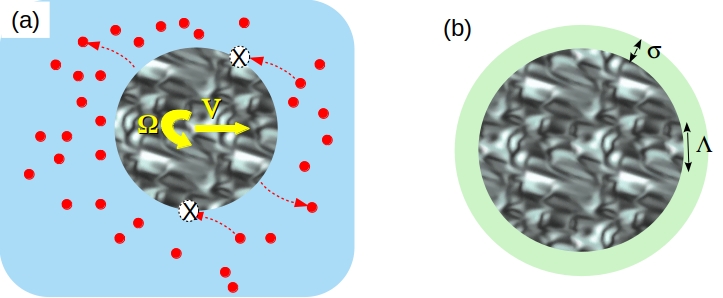
Figure 1: (a) Schematic depiction of the model system. A rigid, impermeable, spherical particle (the central disk), is immersed in a solution composed of solvent (the majority phase, shown as the blue background) and a single species of a molecular solute (the red small disks), which diffuses in the solution. The particle is chemically active, i.e., it releases (or removes) solute molecules into (from) the solution adjacent to the surface. The texture of the particle is an illustrative depiction that its properties (adsorption potential, chemical activity) can vary along the surface. As a result of the coupling of the particle, via the adsorption potential, with the non-equilibrium inhomogeneities in chemical composition induced by the activity, the particle translates with phoretic velocity ${\bf V}$ and rotates with phoretic angular velocity ${\bm{\Omega}}$ (yellow arrows), while the solution flows. (b) The range $\sigma$ of the adsorption potential defines a “diffuse” particle–fluid interface, where the interaction is effective. The lateral variations of particle properties along its surface are characterized by a length scale $\Lambda$.

The field $n({\bf r})$ is determined by particle number conservation for the chemical,

$$\nabla\cdot{\bf j}_{\mathrm{diff}}=0,\qquad{\bf j}_{\mathrm{diff}}=\Gamma\mathbf{f},$$ (2)

in terms of the current ${\bf j}_{\mathrm{diff}}$, the body force density ${\bf f}$ acting on the chemical and which drives its diffusion, and the mobility $\Gamma=D/k_{B}T$ of the chemical in the solution. Consistently with the slow dynamics of the particle, one assumes local equilibrium for the chemical [20, 46, 15, 26, 25, 24], so that

$$\mathbf{f}({\bf r})=-n({\bf r})\nabla\mu({\bf r}),$$ (3)

in terms of its chemical potential $\mu({\bf r})$, modeled by means of a free energy functional [46]:

$$\mathcal{H}[n]=\int\limits_{r>R}d^{3}{\bf r}\;\left[h(n)+n\,\mathbb{W}({\bf r})\right],$$ (4a)

$$\mu({\bf r})=\frac{\delta\mathcal{H}[n]}{\delta n({\bf r})}=h^{\prime}(n({\bf r}))+\mathbb{W}({\bf r}),$$ (4b)

where $h(n)$ is a local free energy density, which depends implicitly also on temperature, and $\mathbb{W}({\bf r})$ is the potential energy associated to the particle–chemical interaction. This potential has a non-zero and finite range and reflects the preference of the particle for one of the components of the solution; it will be accordingly referred to as adsorption potential. We note that the simplest choice for the free energy density $h(n)$, frequently employed in models of phoresis and self-phoresis [20, 22, 29], is that of an ideal gas,

$$h_{\mathrm{id}}(n)=k_{B}T\,n(\ln n-1)\,.$$ (5)

The diffusion equation that follows from Eqs. (2) and (3) is subject to boundary conditions at infinity and at the surface of the particle. We impose that the perturbations due to the particle (through adsorption and chemical activity) remain localized, so that the solution far from the particle is at equilibrium, characterized by a homogeneous chemical density $n_{0}$. At the surface of the particle, the chemical activity of release/remove of chemical into/from the solution is modelled as a chemical current along the direction normal to the particle. Accordingly,

$$\mu(|{\bf r}|\to\infty)\to\mu_{0}=h^{\prime}(n_{0})\,,$$ (6a)

$${\bf e}_{r}\cdot{\bf j}_{\mathrm{diff}}({\bf r}_{p})=\mathcal{A}\,\mathbb{A}({\bf r}_{p})\,,$$ (6b)

where ${\bf r}_{p}$ generically denotes any point on the surface of the particle. The parameter $\mathcal{A}$ is a measure of the magnitude of the chemical activity (e.g., the maximum rate of chemical release or removal over the surface), and the dimensionless surface field $\mathbb{A}({\bf r}_{p})$ is the pattern of surface chemical activity.

The flow field ${\bf u}({\bf r})$ is assumed to be incompressible and determined by the balance between the force field ${\bf f}({\bf r})$, which acts on the solution, and the fluid stresses, as expressed by the incompressible Stokes equation:

$$\eta\nabla^{2}{\bf u}-\nabla p+\mathbf{f}=0,$$ (7a)

$$\nabla\cdot{\bf u}=0,$$ (7b)

where $\eta$ is the viscosity of the solution and $p({\bf r})$ is the hydrodynamic pressure field that enforces incompressibility. The equations are subject to boundary conditions: a vanishing velocity at infinity, that sets the reference frame consistent with the equilibrium state of the solution, and the usual no-slip at the surface of the particle:

$${\bf u}(|{\bf r}|\to\infty)\to 0\,,$$ (8a)

$${\bf u}({\bf r}_{p})={\bf V}+{\bm{\Omega}}\times{\bf r}_{p}\,.$$ (8b)

The quantities ${\bf V}$ and ${\bm{\Omega}}$ are still unknowns. The mathematical problem is closed by the requirement that the composed system “particle + solution” is mechanically isolated, that is, there is no external force or torque acting on the particle (recall that, as follows from Eq. (7a) and the physical meaning of ${\bf f}$ given by Eqs. (3, 4), there are no external forces acting on the fluid). One can then solve Eqs. (2)–(8) in order to derive the velocities ${\bf V}$ and ${\bm{\Omega}}$ in terms of the force field ${\bf f}$.

However, one can sidestep the need to solve the full hydrodynamic problem (7–8) for the flow ${\bf u}$ by applying the reciprocal theorem [47, 28, 31, 44], which provides ${\bf V}$ and ${\bm{\Omega}}$ directly as functionals of the force density (3). The incompressibility constraint (7b) implies that only the solenoidal component of the force density matters. Therefore, instead of the customary expression for ${\bf V},{\bm{\Omega}}$ in terms of the field $\mathbf{f}({\bf r})$, we follow the approach recently proposed in Ref. [44] of using an expression that depends explicitly just on $\nabla\times\mathbf{f}({\bf r})$: this has the advantage that any approximation in the integral representation (which will be unavoidable for further analytical progress or in numerical implementations with finite precision) does not inadvertently carry over a spurious contribution to the motion from a non-solenoidal component of the force. One then introduces one scalar and three vector hydrodynamic potentials, which for a spherical particle take the following form, respectively:

$$\Phi(r)=-\frac{3}{2}R^{2}\left[1-\frac{2}{3}\frac{R}{r}-\frac{1}{3}\left(\frac{r}{R}\right)^{2}\right],$$ (9a)

$${\bf A}^{(k)}({\bf r})=A(r)\,{\bf e}_{k}\times{\bf e}_{r},$$ (9b)

$$A(r):=\frac{3}{4}R\left[1-\frac{2}{3}\frac{r}{R}-\frac{1}{3}\left(\frac{R}{r}\right)^{2}\right],$$ (9c)

in spherical coordinates with the origin at the center of the particle (${\bf e}_{k}$, $k=1,2,3$, are Cartesian unit vectors, and ${\bf e}_{r}$ is the unit radial vector), for which we chose the gauge such that the potentials vanish at the surface of the particle and the fields ${\bf A}^{(k)}$ are solenoidal [44]. By using this approach, one obtains a representation like in Eq. (1a) with the following exact integral representations of the surface fields [31, 44]:

$${\bf v}_{s}({\bf r}_{p})=-\frac{2}{3\eta R}\int\limits_{0}^{\infty}dz\;(R+z)^{2}\,A(R+z)\,{\bf e}_{r}\times\left[\nabla\times{\bf f}({\bf r}_{p}+z{\bf e}_{r})\right],$$ (10a)

$${\bm{\omega}}_{s}({\bf r}_{p})=-\frac{2}{\eta R^{3}}\int\limits_{0}^{\infty}dz\;(R+z)^{2}\,\Phi(R+z)\,\nabla\times{\bf f}({\bf r}_{p}+z{\bf e}_{r}),$$ (10b)

where $z>0$ is the distance from the point ${\bf r}_{p}=R{\bf e}_{r}$ at the surface of the particle (i.e., any point ${\bf r}$ in the fluid is expressed as ${\bf r}=(R+z){\bf e}_{r}$). Notice that the expression (10a) gives a velocity ${\bf v}_{s}$ that is obviously tangential to the surface (the vector ${\bf e}_{r}$ does not depend on $z$). The direction of the other surface field, ${\bm{\omega}}_{s}$, is not evident and one cannot a priori rule out a component along the normal to the surface; however, it turns out that its contribution to the surface average (1) that gives ${\bm{\Omega}}$ involves solely tangential components, see, c.f., Eqs. (29b, 31b). What one can nevertheless show rigorously is that these exact expressions for the fields ${\bf v}_{s}$ and ${\bm{\omega}}_{s}$ are not related like in Eq. (1b).

The expressions (10) are generally valid irrespective of the exact form of the force field ${\bf f}$ or the free energy functional $\mathcal{H}$, see Eqs. (3, 4), i.e., they hold equally well for more complex mechanisms such as the correlation–induced phoresis [31]. For the specific form given by Eq. (4), which depends only locally on $n$ via the free energy density $h(n)$, one has

$$\nabla n=\frac{1}{h^{\prime\prime}(n)}\nabla\left(\mu-\mathbb{W}\right),$$ (11)

so that it holds

$$\nabla\times{\bf f}=-\nabla n\times\nabla\mu=\frac{1}{h^{\prime\prime}(n)}\nabla\mathbb{W}\times\nabla\mu\,.$$ (12)

This expression explicitly highlights that phoretic motion arises by the misalignment between the adsorption force ($\sim\nabla\mathbb{W}$) exerted by the particle on the solute molecules and the non-equilibrium thermodynamic force ($\sim\nabla\mu$) due to the chemical activity.

III The thin–layer and the lubrication approximations

As discussed earlier, in many cases the force density ${\bf f}$ is non-vanishing only in a thin layer at the surface of the particle (the “diffuse interface” [20]). For the form given by Eq. (12), this usually happens when the adsorption potential $\mathbb{W}$ has a range $\sigma$ that is much smaller than the particle size, $\sigma\ll R$. In such case, the radial integrals in Eqs. (10) into the fluid domain are effectively cut off ($z=r-R\lesssim\sigma$) to the layer of fluid within the spherical shell of thickness $\sim\sigma$ around the surface of the particle, see Figure 1(b). Then, one can Taylor–expand the hydrodynamic kernels $\Phi(r),A(r)$ (and the term $(R+z)^{2}$ coming from the volume element) in the variable $z\ll R$ because they only involve the large scale $R$. In this manner, one arrives at the thin–layer approximation for the phoretic velocities:

$${\bf v}_{s}({\bf r}_{p})\approx-\frac{2}{3}{\bf r}_{p}\times{\bm{\omega}}_{s}({\bf r}_{p}),$$ (13a)

$${\bm{\omega}}_{s}({\bf r}_{p})\approx-\frac{3}{4\eta R}\int\limits_{0}^{\infty}dz\;z^{2}\,\nabla\times{\bf f}({\bf r}_{p}+z{\bf e}_{r}).$$ (13b)

Notice that (i) although the integral over $z$ is formally extended to infinity, the fast decay of ${\bf f}$ ensures that only the thin–layer domain contributes, and (ii) because the layer thickness is microscopic compared to the particle size, the fields ${\bf v}_{s}({\bf r}_{p})$ and ${\bm{\omega}}_{s}({\bf r}_{p})$ can be properly called “surface fields”.

So far, the approximation addresses only the behavior of the hydrodynamic kernels based on the scale $\sigma$ of radial variation of the field $\nabla\times\mathbf{f}$. In order to make further progress, we have to study also its variation in the lateral (tangential) direction on the particle’s surface. Let $\Lambda_{\mathbb{W}}$ denote the characteristic scale of lateral variation of the adsorption potential. Introduce the tangential gradient $\nabla_{\parallel}:=\nabla-{\bf e}_{r}\partial_{r}$, so that one can write

$$\nabla\mathbb{W}=\nabla_{\parallel}\mathbb{W}+{\bf e}_{r}\frac{\partial\mathbb{W}}{\partial r}.$$ (14)

One can thus estimate

$$\frac{\left|\partial_{r}\mathbb{W}\right|}{\left|\nabla_{\parallel}\mathbb{W}\right|}\sim\frac{\Lambda_{\mathbb{W}}}{\sigma}.$$ (15)

Therefore, an additional, natural approximation occurs when the lateral variation is slow compared to the variation in the radial direction, i.e., $\sigma\ll\Lambda_{\mathbb{W}}$, so that

$$\nabla\mathbb{W}\approx{\bf e}_{r}\frac{\partial\mathbb{W}}{\partial r},$$ (16)

and Eq. (13) are further simplified, upon using Eq. (12), as

$${\bm{\omega}}_{s}({\bf r}_{p})\approx-\frac{3}{4\eta R}\int\limits_{0}^{\infty}dz\;z^{2}\,\frac{1}{h^{\prime\prime}(n)}\frac{\partial\mathbb{W}}{\partial z}{\bf e}_{r}\times\nabla_{\parallel}\mu,$$ (17a)

$${\bf v}_{s}({\bf r}_{p})\approx-\frac{1}{2\eta}\int\limits_{0}^{\infty}dz\;z^{2}\,\frac{1}{h^{\prime\prime}(n)}\frac{\partial\mathbb{W}}{\partial z}\nabla_{\parallel}\mu.$$ (17b)

Now it is obvious that both fields are tangential and also fulfill Eq. (1b), so that it suffices to focus on the tangential slip velocity ${\bf v}_{s}$ from now on.

At this point, a specific expression of the chemical potential is needed. Unfortunately, even for the simplest case of an ideal gas (5), the diffusion problem (2–6) leads to a complicated partial differential equation that cannot be solved analytically. Accordingly, we now address the case of small deviations from the homogeneous, equilibrium state, for which the governing equations can be simplified.

III.1 The quasi-homogeneous regime

When both $\mathbb{A}=0$ and $\mathbb{W}=0$, the solution represents an equilibrium state characterized by a uniform density $n_{0}$. Therefore, if $\mathbb{A}$ and $\mathbb{W}$ are sufficiently small, one can linearize the governing equations by expanding to first order in the deviations $\delta n:=n-n_{0}$. The diffusion problem reduces to a Laplace boundary value problem for $\delta\mu:=\mu-\mu_{0}$:

$$\nabla^{2}\delta\mu=0,$$ (18a)

$$\delta\mu(|{\bf r}|\to\infty)=0,$$ (18b)

$${\bf e}_{r}\cdot\nabla\delta\mu({\bf r}_{p})=-\frac{\mathcal{A}}{n_{0}\Gamma}\mathbb{A}({\bf r}_{p}),$$ (18c)

and linearization of Eq. (11) then provides

$$\delta n({\bf r})=\frac{1}{h^{\prime\prime}(n_{0})}\left[\delta\mu({\bf r})-\mathbb{W}({\bf r})\right]\,.$$ (19)

Within this approximation, one can set

$$h^{\prime\prime}(n)\approx h^{\prime\prime}(n_{0})$$ (20)

in the integrals appearing in Eqs. (17) and the phoretic velocities appear, to leading order, as quadratic magnitudes in the deviations from the equilibrium state.

For the spherical particle, Eqs. (18) can be solved straightforwardly by expanding the fields in spherical harmonics: if the activity is expressed in terms of dimensionless coefficients $a_{\ell m}$ as

$$\mathbb{A}({\bf r}_{p}=R{\bf e}_{r})=\sum_{\ell m}a_{\ell m}Y_{\ell m}({\bf e}_{r}),$$ (21)

one gets

$$\delta\mu({\bf r}=(R+z){\bf e}_{r})=\frac{\mathcal{A}R}{n_{0}\Gamma}\sum_{\ell m}\nu_{\ell m}(z)\,Y_{\ell m}({\bf e}_{r}).$$ (22a)

in terms of the dimensionless coefficients

$$\nu_{\ell m}(z):=\frac{a_{\ell m}}{\ell+1}\left(1+\frac{z}{R}\right)^{-(\ell+1)}.$$ (22b)

The relevant feature is that the derivatives of the chemical potential in the radial and in the tangential direction are of the same order (this follows directly from the Laplace equation (18a), but it can be checked also with the explicit solution (22), see App. A). Therefore, if the activity pattern $\mathbb{A}({\bf r}_{p})$ has a characteristic scale $\Lambda_{\mathbb{A}}$ of lateral variation on the particle’s surface, so will $\delta\mu$ (via the common coefficients $a_{\ell m}$ appearing in Eqs. (21, 22)), and thus $\Lambda_{\mathbb{A}}$ will also set the scale of radial variation of $\delta\mu$.

III.2 The phoretic coefficient

Assume now that, as happens with the length $\Lambda_{\mathbb{W}}$, also the length scale $\Lambda_{\mathbb{A}}$ is much larger than the thickness $\sigma$ of the diffuse interface. Then, in view of the feature just remarked about the field $\delta\mu({\bf r})$, one can approximate this field by its value at the surface of particle when evaluating the integral in $z$ appearing in Eqs. (17). Therefore, together with the approximation (20), one finally gets

$${\bf v}_{s}({\bf r}_{p})\approx\frac{\mathcal{L}({\bf r}_{p})}{h^{\prime\prime}(n_{0})}\nabla_{\parallel}\delta\mu({\bf r}_{p}),$$ (23a)

in terms of the coefficient

$$\mathcal{L}({\bf r}_{p}) := \mbox{}-\frac{1}{2\eta}\int\limits_{0}^{\infty}dz\;z^{2}\,\frac{\partial\mathbb{W}}{\partial z}({\bf r}_{p}+z{\bf e}_{r})$$ (24)

$$= \frac{1}{\eta}\int\limits_{0}^{\infty}dz\;z\,\mathbb{W}({\bf r}_{p}+z{\bf e}_{r}),$$

after integration by parts. This result can be properly termed the lubrication approximation, see Sec. IV.

In order to illustrate the meaning of $\mathcal{L}$, we notice that it is experimentally much simpler to record gradients in density than in chemical potentials: when evaluating fields outside of the diffuse interface but still close to the particle, i.e., at some value of $z$ such that $\sigma\ll z\ll R$, one can set $\mathbb{W}=0$ and, in particular, Eq. (19) allows one to define the “outer density” as

$$\delta n^{\mathrm{(o)}}({\bf r}):=\frac{\delta\mu({\bf r})}{h^{\prime\prime}(n_{0})}.$$ (25)

Using this relationship to simplify Eqs. (23a), one finally arrives at

$${\bf v}_{s}({\bf r}_{p})=\mathcal{L}({\bf r}_{p})\,\nabla_{\parallel}\delta n^{\mathrm{(o)}}({\bf r}_{p})\,.$$ (26)

One recognizes here the classic expression for the phoretic slip velocity as proportional to the observable “outer” tangential gradient in chemical concentration (be it due to activity or externally imposed), where $\mathcal{L}$ is the phoretic coefficient [19, 20, 29]. Note that Eq. (26) corresponds to the classic result derived for an ideal gas [19, 20],

$$\mathcal{L}_{\mathrm{id}}=\frac{k_{B}T}{\eta}\int\limits_{0}^{\infty}dz\;z\left[1-\exp(-\mathbb{W}/k_{B}T)\right],$$ (27)

in the quasi–homogeneous regime limit $|\mathbb{W}|\ll k_{B}T$; we remark in passing that this result can be derived from Eqs. (17) before implementing the approximation of quasi-homogeneity if one uses the insight that $\mu$ varies little in the radial direction when the conditions for the lubrication approximation hold, see App. B.

IV Beyond the approximations

The lubrication approximation is distinctly different from the thin–layer approximation (13). In the latter, only the curvature of the particle surface is neglected, so that the hydrodynamic flow within the diffuse interface is approximated as if near a flat wall. In the lubrication approximation also the lateral variations of this flow along the surface are neglected, so that the problem is reduced to a shear flow within the diffuse interface and parallel to the particle.

More precisely, the lubrication approximation amounts to claiming that the thickness of the diffuse interface, set by the range $\sigma$ of the adsorption potential in our case, is much smaller than any other length scale that might be relevant for the hydrodynamic flow, be it the curvature radius of the particle or the scale of lateral variation of the fields. It seems natural to explore the possibility of relaxing some of these constraints, particularly in view of the ever improving technical capabilities in the fabrication of active particles. For instance, it is currently feasible to get particles of radii in the range $R\simeq 100~{}\mathrm{nm}$ [48, 49], for which a pattern of alternating active/inactive surface over an angle $\pi/16(\sim 11^{\mathrm{o}})$ renders $\Lambda_{\mathbb{A}},\Lambda_{\mathbb{W}}\sim R/5\simeq 20~{}\mathrm{nm}$; with a typical value $\sigma\simeq 5~{}\mathrm{nm}$, the ratio $\Lambda_{\mathbb{A,W}}/\sigma\sim 4$ is quantitatively significant and it cannot be taken for granted as “very large”, so that it could eventually lead to observable discrepancies from the prediction based on Eq. (26).

In order to address the case when the simplifying approximations discussed above are relaxed, we explore an alternative representation of the phoretic velocities (10) introduced originally in Ref. [31], and which is valid in the quasi-homogeneous regime. By using the expansions (21, 22) and a similar one for the adsorption potential,

$$\mathbb{W}({\bf r}=(R+z){\bf e}_{r})=\mathcal{W}\sum_{\ell m}w_{\ell m}(z)Y_{\ell m}({\bf e}_{r}),$$ (28)

where $\mathcal{W}$ is a characteristic scale of the potential and the coefficients $w_{\ell m}(z)$ are dimensionless, one can write (see App. C)

$${\bf V}=V_{0}\sum_{\ell m}\sum_{\ell^{\prime}m^{\prime}}a_{\ell^{\prime}m^{\prime}}\left\{\left[b_{\ell m;\ell^{\prime}}+\frac{\ell^{\prime}+1}{\ell+1}c_{\ell m;\ell^{\prime}}\right]\,{\bf G}^{\parallel}_{\ell m;\ell^{\prime}m^{\prime}}+c_{\ell m;\ell^{\prime}}\,{\bf G}^{\parallel}_{\ell^{\prime}m^{\prime};\ell m}\right\},$$ (29a)

$${\bm{\Omega}}=\frac{3V_{0}}{2R}\sum_{\ell m}\sum_{\ell^{\prime}m^{\prime}}a_{\ell^{\prime}m^{\prime}}\left[b_{\ell m;\ell^{\prime}-1}+\frac{1}{\ell+1}c_{\ell m;\ell^{\prime}-1}\right]{\bf G}^{\tau}_{\ell m;\ell^{\prime}m^{\prime}},$$ (29b)

with

$$V_{0}=\frac{\mathcal{A}\mathcal{W}R^{2}}{6\pi\eta\Gamma n_{0}h^{\prime\prime}(n_{0})},$$ (30)

a characteristic velocity scale. The dimensionless vectors ${\bf G}^{\parallel,\tau}$ (surface averages of products of spherical harmonics defined in Ref. [31]) are given by

$${\bf G}^{\parallel}_{\ell m;\ell^{\prime}m^{\prime}}:=-\frac{4\pi R}{\ell^{\prime}+1}\left\langle Y_{\ell m}({\bf e}_{r})\,\nabla_{\parallel}Y_{\ell^{\prime}m^{\prime}}({\bf e}_{r})\right\rangle,$$ (31a)

$${\bf G}^{\tau}_{\ell m;\ell^{\prime}m^{\prime}}:=-\frac{4\pi R}{\ell^{\prime}+1}\left\langle Y_{\ell m}({\bf e}_{r})\,{\bf e}_{r}\times\nabla_{\parallel}Y_{\ell^{\prime}m^{\prime}}({\bf e}_{r})\right\rangle,$$ (31b)

and the coefficients $b_{\ell m;\ell^{\prime}}$ and $c_{\ell m;\ell^{\prime}}$ are defined as the following dimensionless radial integrals:

$$b_{\ell m;\ell^{\prime}}:=\int\limits_{0}^{\infty}\frac{dz}{R}\;H^{\mathrm{(b)}}\left(\frac{z}{R}\right)\left(1+\frac{z}{R}\right)^{-\ell^{\prime}}w_{\ell m}(z),$$ (32a)

$$c_{\ell m;\ell^{\prime}}:=-\frac{\ell+1}{2}\int\limits_{0}^{\infty}\frac{dz}{R}\;H^{\mathrm{(c)}}\left(\frac{z}{R}\right)\left(1+\frac{z}{R}\right)^{-\ell^{\prime}}w_{\ell m}(z),$$ (32b)

where the functions $H^{(b,c)}$, which are directly related to the hydrodynamic kernels $A(r)$, $\Phi(r)$ in Eq. (10), are given by

$$H^{\mathrm{(b)}}(\zeta):=1-\frac{3}{4(1+\zeta)}-\frac{1}{4(1+\zeta)^{3}},$$ (33a)

$$H^{\mathrm{(c)}}(\zeta):=1-\frac{3}{2(1+\zeta)}+\frac{1}{2(1+\zeta)^{3}}.$$ (33b)

One can recognize in the definitions (32) a contribution ($w_{\ell m}$) coming from the the adsorption potential and a $z$-dependent term stemming from the solution (22) for the chemical potential).

The most relevant feature concerning the ${\bf G}$ vectors, which by their definition are of the order of unity (when non-vanishing), are the so-called “selection rules” [31]: in the double sum in Eq. (29a), the only terms different from zero are those which satisfy $|\ell-\ell^{\prime}|=1$ and $|m+m^{\prime}|=0$ or $1$, while in Eq. (29b) only those which obey $|\ell-\ell^{\prime}|=0$ and $|m+m^{\prime}|=0$ or $1$. Therefore, and against appearances, Eqs. (29) involve a single series over surface modes (because $\ell-1\leq\ell^{\prime}\leq\ell+1$ and thus effectively the second series is reduced to a few terms sum), each one characterized by a length scale $\Lambda_{\ell}=R/\ell$ of lateral variation. This property already provides an insightful observation: even if the products involving $\mathbb{W}$ and $\mu$ in Eqs. (17) would yield non-vanishing surface fields ${\bf v}_{s}$, ${\bm{\omega}}_{s}$, their contribution to the phoretic velocities is strongly suppressed upon performing the surface average in Eq. (1a) if the fields $\mathbb{W}$ and $\mathbb{A}$ have widely differing scales of lateral variations, i.e., if their respective expansions are dominated by widely different values of $\ell$ and $\ell^{\prime}$, respectively. Therefore, the length scales $\Lambda_{\mathbb{W}}$ and $\Lambda_{\mathbb{A}}$ employed in the reasoning leading to the lubrication approximation must effectively be of the same order. In other words, it is sufficient to require one of the length scales, e.g., $\Lambda_{\mathbb{W}}$, to be much larger than $\sigma$, and the selection rules automatically ensure the proper lubrication approximation in that a non-zero velocity can occur only if the other length scale $\Lambda_{\mathbb{A}}$ is also large.

Assume once more that the coefficients $w_{\ell m}(R+z)$ vanish quickly for separations $z\gtrsim\sigma$ from the surface. The thin–layer approximation is recovered when $\sigma\ll R$, and is expressed in Eqs. (29) by Taylor-expanding the hydrodynamic $H$-functions:

$$H^{\mathrm{(b)}}(\zeta\ll 1)\approx\frac{3\zeta}{2},\quad H^{\mathrm{(c)}}(\zeta\ll 1)\approx\frac{3\zeta^{2}}{2}.$$ (34)

If, in addition, the main contribution to the sums in Eqs. (29) stems from modes with a small value of $\ell$, i.e., modes that vary on the surface over a large scale $\Lambda_{\ell}\sim R/\ell\sim R\gg\sigma$, one can expand $(1+z/R)^{-\ell^{\prime}}\approx 1-\ell^{\prime}z/R=1-z/\Lambda_{\ell^{\prime}}\approx 1$ in the radial integrals. In this case, the coefficient $c_{\ell m;\ell^{\prime}}$ is a factor $\sim(\ell+1)z/R\lesssim\sigma/R$ smaller than $b_{\ell m;\ell^{\prime}}$, and thus the $c$ coefficients can be neglected. In this manner, the lubrication approximation is recovered from Eqs. (29) with the coefficient

$$b^{\mathrm{(lubr)}}_{\ell m;\ell^{\prime}}=\frac{3}{2R^{2}}\int\limits_{0}^{\infty}dz\;z\,w_{\ell m}(z),$$ (35)

compare with the phoretic coefficient (24). The fact that $b_{\ell m;\ell^{\prime}}$ does not actually depend on the index $\ell^{\prime}$ in this approximation reflects the factorization expressed by Eq. (26): in Eqs. (29) the sum over $\ell^{\prime}$ now involves only the activity, while that over $\ell$ only the adsorption potential.

If, however, the sums in Eqs. (29) get significant contributions from modes with $\ell\gg 1$, associated to lateral variations over small scales $\Lambda_{\ell}\sim\sigma$, only the thin–layer approximation (34) is expected to hold. In the radial integrals one could then approximate

$$\left(1+\frac{z}{R}\right)^{-\ell^{\prime}}=\mathrm{e}^{-\ell^{\prime}\ln(1+z/R)}\approx\mathrm{e}^{-\ell^{\prime}z/R}=\mathrm{e}^{-z/\Lambda_{\ell^{\prime}}},$$ (36)

because $z/R\lesssim\sigma/R\ll 1$, and write

$$b^{\mathrm{(thin)}}_{\ell m;\ell^{\prime}}=\frac{3}{2R^{2}}\int\limits_{0}^{\infty}dz\;z\,\mathrm{e}^{-z/\Lambda_{\ell^{\prime}}}\,w_{\ell m}(z),$$ (37a)

$$c^{\mathrm{(thin)}}_{\ell m;\ell^{\prime}}=-\frac{3}{4R^{2}}\int\limits_{0}^{\infty}dz\;\frac{z^{2}}{\Lambda_{\ell}}\,\mathrm{e}^{-z/\Lambda_{\ell^{\prime}}}\,w_{\ell m}(z),$$ (37b)

The relevant feature is the non-trivial dependence of the coefficients on both indices $\ell,\ell^{\prime}$, which prevents a simple factorization as discussed above. Actually, there does not seem to be a simple and appealing description, like the one based on the phoretic coefficient, in the more general case.

Since the integrals appearing in Eqs. (37) do not seem much different from Eq. (35) or Eqs. (32), the question of their relative magnitude naturally arises. By way of example, we consider an adsorption potential modeled as a square–well in the radial direction, so that each mode takes the form ($\hat{w}_{\ell m}$ is $z$-independent)

$$w_{\ell m}(R+z)=\left\{\begin{array}[c]{cl}\hat{w}_{\ell m},&0<z<\sigma,\\ 0,&\sigma<z.\end{array}\right.$$ (38)

Then, the lubrication approximation (35) gives

$$b^{\mathrm{(lubr)}}_{\ell m;\ell^{\prime}}=\frac{3\sigma^{2}}{4R^{2}}\hat{w}_{\ell m},$$ (39)

and the thin–layer approximation (37) yields

$$b^{\mathrm{(thin)}}_{\ell m;\ell^{\prime}}=b^{\mathrm{(lubr)}}_{\ell m;\ell^{\prime}}\;\frac{2\Lambda_{\ell^{\prime}}^{2}}{\sigma^{2}}\left[1-\left(1+\frac{\sigma}{\Lambda_{\ell^{\prime}}}\right)\mathrm{e}^{-\sigma/\Lambda_{\ell^{\prime}}}\right],$$ (40a)

$$c^{\mathrm{(thin)}}_{\ell m;\ell^{\prime}}=-\frac{\ell}{\ell^{\prime}}b^{\mathrm{(lubr)}}_{\ell m;\ell^{\prime}}\;\frac{2\Lambda_{\ell^{\prime}}^{2}}{\sigma^{2}}\left[1-\left(1+\frac{\sigma}{\Lambda_{\ell^{\prime}}}+\frac{\sigma^{2}}{2\Lambda_{\ell^{\prime}}^{2}}\right)\mathrm{e}^{-\sigma/\Lambda_{\ell^{\prime}}}\right].$$ (40b)

Figure 2(left) compares the coefficients in the lubrication or in the thin–layer approximations, respectively, as a function of the ratio $\Lambda_{\ell^{\prime}}/\sigma$ (with the choice $\ell^{\prime}=\ell$, since the selection rules imply that they must have similar values to contribute to the velocity). One can straightforwardly infer that the changes are rather mild even at small values of $\Lambda_{\ell^{\prime}}$; thus one concludes that the results of the lubrication approximation may provide reasonable estimates for the velocity even in conditions under which the underlying approximations are not expected to hold.

One can also compare with the exact results that follow from Eqs. (32), i.e., before any assumption is made on the relative magnitude of the adsorption range $\sigma$ and the radius $R$. Although the integrals can be evaluated exactly for the choice (38), the results are lengthy and not very illuminating, and we do not deem necessary to present them. For illustration, Fig. 2(right) shows the comparison of the exact results with the lubrication approximation as a function of the ratio $R/\sigma$ in two representative cases, namely, when the scale of lateral variation verifies $\Lambda_{\ell^{\prime}}\sim R$, and when it is $\Lambda_{\ell^{\prime}}\sim\sigma$, respectively. The conclusion that follows from Fig. (2) is that there are not major quantitative changes when different approximations are considered provided the range $\sigma$ and the scales of lateral variation are smaller or comparable to the particle radius.

It thus seems that, as far as the quantitative value of the radial coefficients (32) is concerned, one could use the lubrication approximation in order to get good estimates even beyond its expected range of validity. Although this insight is based on the specific choice of a square–well adsorption potential (38), one can arguably expect it to hold for more generic forms that have a single characteristic scale $\sigma$ of smooth variation.

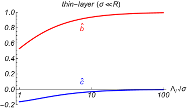
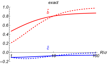
Figure 2: Plot of the ratios $\hat{b}:=b_{\ell m;\ell^{\prime}}/b^{\mathrm{(lubr)}}_{\ell m;\ell^{\prime}}$ (red curves) and $\hat{c}:=c_{\ell m;\ell^{\prime}}/b^{\mathrm{(lubr)}}_{\ell m;\ell^{\prime}}$ (blue curves). The results do not depend on the index $m$, the dependence on $\ell^{\prime}$ is parametrized in terms of the length $\Lambda_{\ell^{\prime}}=R/\ell^{\prime}$, and $\ell=\ell^{\prime}$ is taken for simplicity in evaluating Eqs. (32b, 40b) for the coefficient $c_{\ell m;\ell^{\prime}}$ (since $|\ell-\ell^{\prime}|\leq 1$ anyhow by the selection rules). (Left panel) The thin–layer approximation given by Eqs. (40), as a function of $\Lambda_{\ell^{\prime}}/\sigma$. In the limit $\Lambda_{\ell^{\prime}}\gg\sigma$ one recovers the lubrication approximation (35) (with a negligible value of the $c$-coefficient). (Right panel) The exact values given by Eqs. (32): the dashed lines correspond to the choice $\Lambda_{\ell^{\prime}}=R/2$ (i.e., $\ell^{\prime}=2$), the full lines to $\Lambda_{\ell^{\prime}}=5\sigma$. In the limit $R\gg\sigma$ one recovers the lubrication approximation (dashed lines) or just the thin–layer approximation (full lines).

V Conclusions

By using the case of a spherical active particle, whose activity consists in releasing or removing a solute and moves by self-chemophoresis, we re-examined the analysis of the rigid-body motion under the assumption of a thin diffuse-layer by employing an integral representation. This allowed us to decouple two steps of approximation: the thin diffuse interface (“thin layer”) and the lubrication (slow variations along the tangential direction) for the adsorption potential, which in general have been implicitly combined by calculations in a planar geometry. Consequently, this permits a straightforward, systematic analysis of the motion in each of the two regimes of interest defined by whether or not the lubrication approximation for the adsorption potential holds.

The lubrication approximation means that the range of the adsorption potential is much smaller larger than any other relevant length scale of the model. In this approximation and under the assumption of small deviations from the equilibrium state (“quasi–homogeneity”), the approach provides a very simple, straightforward derivation of the classic expressions for a phoretic slip velocity in terms of a phoretic coefficient. A potential line of further research consists in relaxing the hypothesis of quasi–homogeneity: this has been done so far only for an ideal gas, which leads to the classical non-linear dependence of the phoretic coefficient on the adsorption potential. It seems worth exploring how this latter result is affected by solute–solute interactions.

One can also relax the lubrication approximation by allowing variations of the adsorption potential over the surface on a length scale comparable with the thickness of the diffuse interface. This case has been addressed explicitly in this work and our analysis suggests that the phoretic velocities would not change much quantitatively. But then, this prompts the study of the opposite limit, namely, when the range of the adsorption potential is significantly larger than any other length scale, particularly, the particle radius.

We expect that the analysis and the results presented in this paper will provide a further impetus to the theoretical interest in the issue of self-phoresis, as well as motivation for experimental studies focused on active particles with patterned surfaces engineered at small scales, both for a validation of the theoretical predictions and, more importantly, as a step towards investigating the intriguing case of “no diffuse interface” mentioned above.

Appendix A Spatial variation of $\delta\mu$

The Laplace equation (18a) can be obtained from a variational principle as an extremum of the functional

$$\mathcal{S}[\mu]=\int\limits_{r>R}d^{3}{\bf r}\;\frac{1}{2}|\nabla\mu|^{2}=\int\limits_{r>R}d^{3}{\bf r}\;\frac{1}{2}\left[\left(\frac{\partial\mu}{\partial r}\right)^{2}+|\nabla_{\parallel}\mu|^{2}\right],$$ (41)

so that, for non-trivial solutions, one may expect $|\partial_{r}\mu|\sim|\nabla_{\parallel}\mu|$ in order of magnitude. Alternatively, one can estimate these magnitudes thorough the surface average of their squares evaluated with the explicit solution (22) on the surface ($z=0$). It follows directly from the boundary condition (18c) that

$$\left\langle|\partial_{r}\mu|^{2}\right\rangle=\left(\frac{\mathcal{A}}{n_{0}\Gamma}\right)^{2}\left\langle|\mathbb{A}|^{2}\right\rangle=\left(\frac{\mathcal{A}}{n_{0}\Gamma}\right)^{2}\sum_{\ell m}\frac{|a_{\ell m}|^{2}}{4\pi}.$$ (42)

For the lateral variation, one has

$$\left\langle|\nabla_{\parallel}\mu|^{2}\right\rangle=\left(\frac{\mathcal{A}R}{n_{0}\Gamma}\right)^{2}\sum_{\ell m}\sum_{\ell^{\prime}m^{\prime}}\nu_{\ell m}(0)\nu_{\ell^{\prime}m^{\prime}}(0)\left\langle\left(\nabla_{\parallel}Y_{\ell m}^{*}\right)\cdot\left(\nabla_{\parallel}Y_{\ell^{\prime}m^{\prime}}\right)\right\rangle.$$ (43)

One can exploit the properties of the spherical harmonics (orthonormality and eigenfunctions of $\nabla_{\parallel}^{2}$):

$$\left\langle\left(\nabla_{\parallel}Y_{\ell m}^{*}\right)\cdot\left(\nabla_{\parallel}Y_{\ell^{\prime}m^{\prime}}\right)\right\rangle = \left\langle\nabla_{\parallel}\cdot\left(Y_{\ell m}^{*}\nabla_{\parallel}Y_{\ell^{\prime}m^{\prime}}\right)\right\rangle-\left\langle Y_{\ell m}^{*}\nabla_{\parallel}^{2}Y_{\ell^{\prime}m^{\prime}}\right\rangle$$ (44)

$$= \frac{\ell^{\prime}(\ell^{\prime}+1)}{R^{2}}\left\langle Y_{\ell m}^{*}\,Y_{\ell^{\prime}m^{\prime}}\right\rangle=\frac{\ell^{\prime}(\ell^{\prime}+1)}{4\pi R^{2}}\delta_{\ell\ell^{\prime}}\delta_{mm^{\prime}},$$

where in the first line the first average vanishes by virtue of Gauss theorem on curved manifolds. Therefore, Eq. (43) becomes

$$\left\langle|\nabla_{\parallel}\mu|^{2}\right\rangle=\left(\frac{\mathcal{A}}{n_{0}\Gamma}\right)^{2}\sum_{\ell m}\frac{\ell}{\ell+1}\frac{|a_{\ell m}|^{2}}{4\pi},$$ (45)

after using Eq. (22b), and one can estimate the ratio

$$\frac{\left\langle|\nabla_{\parallel}\mu|^{2}\right\rangle}{\left\langle|\partial_{r}\mu|^{2}\right\rangle}=1-\frac{\sum_{\ell m}(\ell+1)^{-1}|a_{\ell m}|^{2}}{\sum_{\ell m}|a_{\ell m}|^{2}},$$ (46)

which will be typically of order unity, particularly when the sum is dominated by small scales of lateral variation ($\ell\gg 1$).

Appendix B The ideal gas

For an ideal gas, the following relationship holds according to Eqs. (4b, 5):

$$n=\mathrm{exp}\left(\frac{\mu-\mathbb{W}}{kT}\right),\qquad h^{\prime\prime}(n)=\frac{kT}{n}.$$ (47)

Therefore, one can write the integrand in Eq. (17b) as

$$\frac{1}{h^{\prime\prime}(n)}\frac{\partial\mathbb{W}}{\partial z}\nabla_{\parallel}\mu=kT\frac{\partial}{\partial z}\left(1-\mathrm{e}^{-\mathbb{W}/kT}\right)\,\nabla_{\parallel}\mathrm{e}^{\mu/kT}.$$ (48)

One can now argue as in Sec. III.2: if the integral is effectively cut off at a distance of the order of the range $\sigma$ of $\mathcal{W}$, and one can argue that $\mu$ varies over a much larger length scale, one can approximate

$${\bf v}_{s}({\bf r}_{p})\approx\mathcal{L}_{\mathrm{id}}({\bf r}_{p})\;\nabla_{\parallel}\mathrm{e}^{\mu({\bf r}_{p})/kT},$$ (49)

with

$$\mathcal{L}_{\mathrm{id}}({\bf r}_{p}):=-\frac{kT}{2\eta}\int\limits_{0}^{\infty}dz\;z^{2}\,\frac{\partial}{\partial z}\left(1-\mathrm{e}^{-\mathbb{W}/kT}\right).$$ (50)

Outside of the thin layer, where $\mathbb{W}\approx 0$, one can define the “outer density” as $n^{\mathrm{(o)}}=\mathrm{e}^{\mu({\bf r}_{p})/kT}$ by Eq. (47), so that one arrives at Eq. (26) with the phoretic coefficient given by Eq. (27) after integrating by parts in Eq. (50).

Appendix C Expansion in spherical harmonics

When the definitions (10) are used to compute the surface averages (1a), one gets

$${\bf V}=\frac{2}{3\eta R}\int\limits_{0}^{\infty}dz\;(R+z)^{2}\,A(R+z)\,\langle{\bf e}_{r}\times\left(\nabla\times{\bf f}\right)\rangle,$$ (51a)

$${\bm{\Omega}}=\frac{2}{\eta R^{3}}\int\limits_{0}^{\infty}dz\;(R+z)^{2}\,\Phi(R+z)\,\langle\nabla\times{\bf f}\rangle,$$ (51b)

since the dependence on the position ${\bf e}_{r}$ on the particle’s surface enters only through $\nabla\times{\bf f}$. It will turn out convenient to redefine the tangential gradient $\nabla_{\parallel}$, by making explicit the dependence on the radial coordinate $r$, as

$$\tilde{\nabla}_{\parallel}:=r\nabla_{\parallel}={\bf e}_{\theta}\partial_{\theta}+\frac{{\bf e}_{\varphi}}{\sin\theta}\partial_{\varphi}$$ (52)

in spherical coordinates. With this redefinition, one can approximate Eq. (12) in the quasi-homogeneous approximation as

$$\nabla\times{\bf f} \approx \frac{1}{h^{\prime\prime}(n_{0})}\nabla\mathbb{W}\times\nabla\mu$$ (53)

$$= \frac{1}{h^{\prime\prime}(n_{0})r^{2}}\left[r\frac{\partial\mathbb{W}}{\partial r}{\bf e}_{r}\times\tilde{\nabla}_{\parallel}\mu-r\frac{\partial\mu}{\partial r}{\bf e}_{r}\times\tilde{\nabla}_{\parallel}\mathbb{W}+\tilde{\nabla}_{\parallel}\mathbb{W}\times\tilde{\nabla}_{\parallel}\mu\right],$$

so that one also has

$${\bf e}_{r}\times\left(\nabla\times{\bf f}\right)\approx\frac{1}{h^{\prime\prime}(n_{0})r}\left[\frac{\partial\mu}{\partial r}\,\tilde{\nabla}_{\parallel}\mathbb{W}-\frac{\partial\mathbb{W}}{\partial r}\,\tilde{\nabla}_{\parallel}\mu\right].$$ (54)

These fields can be evaluated by inserting the expansions (22, 28), and when the result is used in Eqs. (51), one gets the following expansions:

$${\bf V}=\frac{2\mathcal{A}\mathcal{W}}{3\eta\Gamma n_{0}h^{\prime\prime}(n_{0})} \displaystyle\sum_{\ell m}\sum_{\ell^{\prime}m^{\prime}} \left\{\left\langle Y_{\ell^{\prime}m^{\prime}}\tilde{\nabla}_{\parallel}Y_{\ell m}\right\rangle\int\limits_{0}^{\infty}dz\;(R+z)\,A(R+z)\frac{d\nu_{\ell^{\prime}m^{\prime}}}{dz}\,w_{\ell m}(z)\right.$$

$$-\left.\left\langle Y_{\ell m}\tilde{\nabla}_{\parallel}Y_{\ell^{\prime}m^{\prime}}\right\rangle\int\limits_{0}^{\infty}dz\;(R+z)\,A(R+z)\frac{dw_{\ell m}}{dz}\,\nu_{\ell^{\prime}m^{\prime}}(z)\right\},$$

$${\bm{\Omega}}=\frac{2\mathcal{A}\mathcal{W}}{\eta\Gamma n_{0}h^{\prime\prime}(n_{0})R^{2}} \displaystyle\sum_{\ell m}\sum_{\ell^{\prime}m^{\prime}} \left\{\left\langle Y_{\ell m}\;{\bf e}_{r}\times\tilde{\nabla}_{\parallel}Y_{\ell^{\prime}m^{\prime}}\right\rangle\int\limits_{0}^{\infty}dz\;(R+z)\,\Phi(R+z)\frac{dw_{\ell m}}{dz}\,\nu_{\ell^{\prime}m^{\prime}}(z)\right.$$

$$-\left\langle Y_{\ell^{\prime}m^{\prime}}\;{\bf e}_{r}\times\tilde{\nabla}_{\parallel}Y_{\ell m}\right\rangle\int\limits_{0}^{\infty}dz\;(R+z)\,\Phi(R+z)\frac{d\nu_{\ell^{\prime}m^{\prime}}}{dz}\,w_{\ell m}(z)$$

$$\left.+\left\langle\left(\tilde{\nabla}_{\parallel}Y_{\ell m}\right)\times\left(\tilde{\nabla}_{\parallel}Y_{\ell^{\prime}m^{\prime}}\right)\right\rangle\int\limits_{0}^{\infty}dz\;\Phi(R+z)\;w_{\ell m}(z)\,\nu_{\ell^{\prime}m^{\prime}}(z)\right\}.$$

Consider first Eq. (55): using the definitions (22b, 30, 31a) and one can identify from the first summand the coefficient

$$c_{\ell m;\ell^{\prime}}:=(\ell+1)\int\limits_{0}^{\infty}d\zeta\;\frac{A(R(1+\zeta))}{R}\,(1+\zeta)^{-\ell^{\prime}-1}\,w_{\ell m}(R\zeta),$$ (56)

appearing in Eq. (29a), in terms of the integration variable $\zeta:=z/R$. In the second summand one can integrate by parts (notice that the hydrodynamic kernel $A(R+z)$ vanishes at $z=0$ and that, by assumption, the coefficients $w_{\ell m}(z)$ vanish at $z\to\infty$ sufficiently fast), so that only the derivatives of $\nu_{\ell^{\prime}m^{\prime}}$ appear,

$$\frac{d\nu_{\ell^{\prime}m^{\prime}}}{dz}=-\frac{a_{\ell^{\prime}m^{\prime}}}{R}\left(1+\frac{z}{R}\right)^{-(\ell^{\prime}+2)}.$$ (57)

In this manner one identifies the other coefficient,

$$b_{\ell m;\ell^{\prime}}:=-\int\limits_{0}^{\infty}d\zeta\;\frac{d}{d\zeta}\left[(1+\zeta)\frac{A(R(1+\zeta))}{R}\right]\;(1+\zeta)^{-\ell^{\prime}-1}\,w_{\ell m}(R\zeta).$$ (58)

By inserting the form (9c) of the hydrodynamic kernel in these expressions, one eventually arrives at Eqs. (32) with the functions given by Eqs. (33).

Addressing now Eq. (55), one notices the following identities (see App. D):

$$\left\langle Y_{\ell^{\prime}m^{\prime}}\;{\bf e}_{r}\times\tilde{\nabla}_{\parallel}Y_{\ell m}\right\rangle=-\left\langle Y_{\ell m}\;{\bf e}_{r}\times\tilde{\nabla}_{\parallel}Y_{\ell^{\prime}m^{\prime}}\right\rangle,$$ (59a)

$$\left\langle\left(\tilde{\nabla}_{\parallel}Y_{\ell m}\right)\times\left(\tilde{\nabla}_{\parallel}Y_{\ell^{\prime}m^{\prime}}\right)\right\rangle=\frac{1}{R}\left\langle Y_{\ell m}\;{\bf e}_{r}\times\tilde{\nabla}_{\parallel}Y_{\ell^{\prime}m^{\prime}}\right\rangle.$$ (59b)

Using them together with the definitions (22b, 30, 31b) and integration by parts as before, one obtains

$${\bm{\Omega}}=\frac{3V_{0}}{2R}\sum_{\ell m}\sum_{\ell^{\prime}m^{\prime}}a_{\ell^{\prime}m^{\prime}}d_{\ell m;\ell^{\prime}}{\bf G}^{\tau}_{\ell m;\ell^{\prime}m^{\prime}},$$ (60)

with coefficients

$$d_{\ell m;\ell^{\prime}}:=\int\limits_{0}^{\infty}d\zeta\;\left\{\frac{d}{d\zeta}\left[(1+\zeta)\frac{\Phi(R(1+\zeta))}{R^{2}}-\frac{\Phi(R(1+\zeta))}{R^{2}}\right]\right\}(1+\zeta)^{-\ell^{\prime}-1}\,w_{\ell m}(R\zeta).$$ (61)

This expression can be evaluated by inserting the form (9a) of the hydrodynamic kernel. Against appearances, it is not independent of the coefficients (56, 58) and it can be expressed as a linear combination of them:

$$d_{\ell m;\ell^{\prime}}=\int\limits_{0}^{\infty}d\zeta\;\left[1-\frac{1}{(1+\zeta)^{3}}\right](1+\zeta)^{1-\ell^{\prime}}w_{\ell m}(\zeta)=b_{\ell m;\ell^{\prime}-1}+\frac{c_{\ell m;\ell^{\prime}-1}}{\ell+1},$$ (62)

and so is Eq. (29b) recovered.

Appendix D Some integral identities

Here we derive some useful identities for averages over the surface of a sphere. In this appendix, $f({\bf e}_{r})$, $g({\bf e}_{r})$ will denote any two smooth functions defined on the sphere $\mathbb{S}_{2}$. The first identity follows from Stokes theorem for a scalar field:

$$\int\limits_{\mathbb{S}_{2}}dS\;{\bf e}_{r}\times\nabla_{\parallel}f=\int\limits_{\mathbb{S}_{2}}d{\bf S}\times\nabla f=\oint\limits_{\partial\mathbb{S}_{2}}d\bm{\ell}\;f=0,$$ (63)

taking into account that a sphere is a closed surface, i.e., it has no boundary: $\partial\mathbb{S}_{2}=\emptyset$. Therefore, one has

$$\langle g\,{\bf e}_{r}\times\nabla_{\parallel}f\rangle=\langle{\bf e}_{r}\times\nabla_{\parallel}(gf)\rangle-\langle f\,{\bf e}_{r}\times\nabla_{\parallel}g\rangle=-\langle f\,{\bf e}_{r}\times\nabla_{\parallel}g\rangle.$$ (64)

This identity demonstrates Eq. (59a). Incidentally, this implies that ${\bf G}^{\tau}_{\ell m;\ell m}=0$.

In order to proof Eq. (59b) one uses the explicit representation (52) and integrates by parts on the surface, accounting that the fields are assumed to be well defined on the whole sphere, and thus must be periodic, in order to drop boundary terms:

$$\langle(\nabla_{\parallel}g)\times(\nabla_{\parallel}f)\rangle = \frac{1}{r^{2}}\left\langle\frac{{\bf e}_{r}}{\sin\theta}\left[(\partial_{\theta}g)(\partial_{\varphi}f)-(\partial_{\varphi}g)(\partial_{\theta}f)\right]\right\rangle$$ (65)

$$= \frac{1}{r^{2}}\left\langle{\bf e}_{\varphi}\,g\,(\partial_{\theta}f)-\frac{{\bf e}_{\theta}}{\sin\theta}g\,(\partial_{\varphi}f)\right\rangle=\frac{1}{r}\left\langle g\;{\bf e}_{r}\times\nabla_{\parallel}f\right\rangle.$$

Finally, the following identity can be proofed also by explicit evaluation:

$$\langle\nabla_{\parallel}f\rangle=\frac{2}{r}\langle{\bf e}_{r}\,f\rangle.$$ (66)

As a consequence, it holds that

$$\left\langle Y_{\ell m}\nabla_{\parallel}Y_{\ell^{\prime}m^{\prime}}\right\rangle=\frac{2}{R}\left\langle{\bf e}_{r}Y_{\ell m}Y_{\ell^{\prime}m^{\prime}}\right\rangle-\left\langle Y_{\ell^{\prime}m^{\prime}}\nabla_{\parallel}Y_{\ell m}\right\rangle.$$ (67)

This yields the following equality:

$$-(\ell^{\prime}+1){\bf G}^{\parallel}_{\ell m;\ell^{\prime}m^{\prime}}=2{\bf G}^{\perp}_{\ell m;\ell^{\prime}m^{\prime}}+(\ell+1){\bf G}^{\parallel}_{\ell^{\prime}m^{\prime};\ell m},$$ (68)

in terms of the vectors

$${\bf G}^{\perp}_{\ell m;\ell^{\prime}m^{\prime}}:=4\pi\left\langle{\bf e}_{r}Y_{\ell m}Y_{\ell^{\prime}m^{\prime}}\right\rangle$$ (69)

introduced in Ref. [31].

References

- Ebbens and Howse [2010] S. J. Ebbens and J. R. Howse, In pursuit of propulsion at the nanoscale, Soft Matter 6, 726 (2010).
- Bechinger et al. [2016] C. Bechinger, R. D. Leonardo, H. Löwen, C. Reichhardt, G. Volpe, and G. Volpe, Active particles in complex and crowded environments, Rev. Mod. Phys. 88, 045006 (2016).
- Dey et al. [2016] K. K. Dey, F. Wong, A. Altemose, and A. Sen, Catalytic motors—Quo Vadimus?, Curr. Op. Colloid Interf. Sci. 21, 4 (2016).
- Gompper et al. [2020] G. Gompper, R. G. Winkler, T. Speck, A. Solon, C. Nardini, F. Peruani, H. Löwen, R. Golestanian, U. B. Kaupp, L. Alvarez, T. Kiorboe, E. Lauga, W. C. K. Poon, A. DeSimone, S. Muiños-Landin, A. Fischer, N. A. Söker, F. Cichos, R. Kapral, P. Gaspard, M. Ripoll, F. Sagues, A. Doostmohammadi, J. M. Yeomans, I. S. Aranson, C. Bechinger, H. Stark, C. K. Hemelrijk, F. J. Nedelec, T. Sarkar, T. Aryaksama, M. Lacroix, G. Duclos, V. Yashunsky, P. Silberzan, M. Arroyo, and S. Kale, The 2020 motile active matter roadmap, J. Phys. Condens. Matt. 32, 193001 (2020).
- Palacci et al. [2013] J. Palacci, S. Sacanna, A. P. Steinberg, D. J. Pine, and P. M. Chaikin, Living crystals of light-activated colloidal surfers, Science 339, 936 (2013).
- Aubret et al. [2018] A. Aubret, M. Youssef, S. Sacanna, and J. Palacci, Targeted assembly and synchronization of self-spinning microgears, Nature Phys. 14, 1114 (2018).
- Maggi et al. [2016] C. Maggi, J. Simmchen, F. Saglimbeni, J. Katuri, M. Dipalo, F. De Angelis, S. Sanchez, and R. Di Leonardo, Self-assembly of micromachining systems powered by Janus micromotors, Small 12, 446 (2016).
- Sundararajan et al. [2008] S. Sundararajan, P. E. Lammert, A. W. Zudans, V. H. Crespi, and A. Sen, Catalytic motors for transport of colloidal cargo, Nano Letters 8, 1271 (2008).
- Baraban et al. [2012] L. Baraban, M. Tasinkevych, M. N. Popescu, S. Sanchez, S. Dietrich, and O. Schmidt, Transport of cargo by catalytic Janus micro-motors, Soft Matter 8, 48 (2012).
- Duan et al. [2015] W. Duan, W. Wang, S. Das, V. Yadav, T. E. Mallouk, and A. Sen, Synthetic nano- and micromachines in analytical chemistry: Sensing, migration, capture, delivery, and separation, Annu. Rev. Analyt. Chem. 8, 311 (2015).
- Katuri et al. [2018] J. Katuri, D. Caballero, R. Voituriez, J. Samitier, and S. Sánchez, Directed flow of micromotors through alignment interactions with micropatterned ratchets, ACS Nano 12, 7282 (2018).
- Bekir et al. [2023] M. Bekir, M. Sperling, D. V. Muñoz, C. Braksch, A. Böker, N. Lomadze, M. N. Popescu, and S. Santer, Versatile microfluidics separation of colloids by combining external flow with light-induced chemical activity, Advanced Materials 35, 2300358 (2023).
- Paxton et al. [2004] W. F. Paxton, K. C. Kistler, C. C. Olmeda, A. Sen, S. K. St. Angelo, Y. Y. Cao, T. E. Mallouk, P. E. Lammert, and V. H. Crespi, Catalytic nanomotors: Autonomous movement of striped nanorods, J. Am. Chem. Soc. 126, 13424 (2004).
- Fournier-Bidoz et al. [2005] S. Fournier-Bidoz, A. C. Arsenault, I. Manners, and G. A. Ozin, Synthetic self-propelled nanorotors, Chem. Commun. 0, 441 (2005).
- Golestanian et al. [2005] R. Golestanian, T. B. Liverpool, and A. Ajdari, Propulsion of a molecular machine by asymmetric distribution of reaction products, Phys. Rev. Lett. 94, 220801 (2005).
- Simmchen et al. [2016] J. Simmchen, J. Katuri, W. E. Uspal, M. N. Popescu, M. Tasinkevych, and S. Sánchez, Topographical pathways guide chemical microswimmers, Nat. Comm. 7, 10598:1 (2016).
- Volpe et al. [2011] G. Volpe, I. Buttinoni, D. Vogt, H.-J. Kümmerer, and C. Bechinger, Microswimmers in patterned environments, Soft Matter 7, 8810 (2011).
- Kroy et al. [2016] K. Kroy, D. Chakraborty, and F. Cichos, Hot microswimmers, Eur. Phys. J. Spec. Topics 225, 2207 (2016).
- Derjaguin et al. [1947] B. V. Derjaguin, G. Sidorenkov, E. Zubashchenkov, and E. Kiseleva, Kinetic phenomena in boundary films of liquids, Kolloidn. Zh. 9, 335 (1947).
- Anderson [1989] J. L. Anderson, Colloid transport by interfacial forces, Annu. Rev. Fluid Mech. 21, 61 (1989).
- Ruckner and Kapral [2007] G. Ruckner and R. Kapral, Chemically powered nanodimers, Phys. Rev. Lett. 98, 150603:1 (2007).
- Golestanian et al. [2007] R. Golestanian, T. B. Liverpool, and A. Ajdari, Designing phoretic micro- and nano-swimmers, New J. Phys. 9, 126:1 (2007).
- Moran and Posner [2017] J. L. Moran and J. D. Posner, Phoretic self-propulsion, Annu. Rev. Fluid Mech. 49, 511 (2017).
- Würger [2015] A. Würger, Self-diffusiophoresis of Janus particles in near-critical mixtures, Phys. Rev. Lett. 115, 188304:1 (2015).
- Samin and van Roij [2015] S. Samin and R. van Roij, Self-propulsion mechanism of active Janus particles in near-critical binary mixtures, Phys. Rev. Lett. 115, 188305:1 (2015).
- Brown et al. [2017] A. T. Brown, W. C. K. Poon, C. Holm, and J. de Graaf, Ionic screening and dissociation are crucial for understanding chemical self-propulsion in polar solvents, Soft Matter 13, 1200 (2017).
- Sharifi-Mood et al. [2013] N. Sharifi-Mood, J. Koplik, and C. Maldarelli, Diffusiophoretic self-propulsion of colloids driven by a surface reaction: The sub-micron particle regime for exponential and van der Waals interactions, Phys. Fluids 25, 012001:1 (2013).
- Sabass and Seifert [2012] B. Sabass and U. Seifert, Dynamics and efficiency of a self-propelled, diffusiophoretic swimmer, J. Chem. Phys. 136, 064508:1 (2012).
- Michelin and Lauga [2014] S. Michelin and E. Lauga, Phoretic self-propulsion at finite péclet numbers, J. Fluid Mech. 747, 572 (2014).
- Popescu et al. [2016] M. Popescu, W. Uspal, and S. Dietrich, Self-diffusiophoresis of chemically active colloids, Eur. Phys. J. Spec. Top. 225, 2189 – 2206 (2016).
- Domínguez et al. [2020] A. Domínguez, M. N. Popescu, C. M. Rohwer, and S. Dietrich, Self-motility of an active particle induced by correlations in the surrounding solution, Phys. Rev. Lett 125, 268002 (2020).
- De Corato et al. [2020] M. De Corato, X. Arqué, T. Patiño, M. Arroyo, S. Sánchez, and I. Pagonabarraga, Self-propulsion of active colloids via ion release: Theory and experiments, Phys. Rev. Lett. 124, 108001 (2020).
- Domínguez and Popescu [2022] A. Domínguez and M. N. Popescu, A fresh view on phoresis and self-phoresis, Curr. Op. Colloid Interf. Sci. 61, 101610 (2022).
- Shreshta and de la Cruz [2024] A. Shreshta and M. de la Cruz, Enhanced phoretic self-propulsion of active colloids through surface charge asymmetry, Phys. Rev. E 109, 014613 (2024).
- Domínguez and Popescu [2024] A. Domínguez and M. Popescu, Ionic self-phoresis maps onto correlation–-induced self-phoresis, arXiv:2404.16435 (2024).
- Gupta et al. [2019] A. Gupta, B. Rallabandi, and H. A. Stone, Diffusiophoretic and diffusioosmotic velocities for mixtures of valence-asymmetric electrolytes, Phys. Rev. Fluids 4, 043702 (2019).
- Wilson et al. [2020] J. L. Wilson, S. Shim, Y. E. Yu, A. Gupta, and H. A. Stone, Diffusiophoresis in multivalent electrolytes, Langmuir 36, 7014 (2020).
- Warren [2020] P. B. Warren, Non-faradaic electric currents in the Nernst-Planck equations and nonlocal diffusiophoresis of suspended colloids in crossed salt gradients, Phys. Rev. Lett. 124, 248004 (2020).
- Williams et al. [2024] I. Williams, P. B. Warren, R. P. Sear, and J. L. Keddie, Colloidal diffusiophoresis in crossed electrolyte gradients: Experimental demonstration of an “action-at-a-distance” effect predicted by the nernst-planck equations, Phys. Rev. Fluids 9, 014201 (2024).
- Happel and Brenner [1965] J. Happel and H. Brenner, Low Reynolds Number Hydrodynamics (Prentice-Hall, Englewood Cliffs, NJ, 1965).
- Kim and Karrila [1991] S. Kim and S. J. Karrila, Microhydrodynamics: Principles and Selected Applications (Butterworth–Heinemann, New York, 1991).
- Lorentz [1896] H. A. Lorentz, Eene algemeene stelling omtrent de beweging eener vloeistof met wrijving en eenige daaruit afgeleide gevolgen, Zittingsverslag van de Koninklijke Akademie van Wetenschappen te Amsterdam 5, 168 (1896).
- Kuiken [1996] H. K. Kuiken, H.A. Lorentz: A general theorem on the motion of a fluid with friction and a few results derived from it (translated from Dutch by H.K. Kuiken), J. Eng. Math. 30, 19 (1996).
- Domínguez and Popescu [2024] A. Domínguez and M. N. Popescu, A representation of the velocity of a rigid particle in a forced stokes flow, Phys. Rev. Fluids , in preparation (2024).
- de Groot and Mazur [1984] S. R. de Groot and P. Mazur, Non-Equilibrium Thermodynamics (Dover, New York, 1984).
- Anderson et al. [1998] D. M. Anderson, G. B. McFadden, and A. A. Wheeler, Diffuse-interface methods in fluid mechanics, Annu. Rev. Fluid Mech. 30, 139 (1998).
- Teubner [1982] M. Teubner, Motion of charged colloidal particles, J. Chem. Phys. 76, 5564 (1982).
- Kim et al. [2017] J. T. Kim, U. Choudhury, J. Hyeon-Ho, and P. Fischer, Nanodiamonds that swim, Adv. Mater. 29, 1701024 (2017).
- Hortelao et al. [2021] A. C. Hortelao, C. Simó, M. Guix, S. Guallar-Garrido, E. Julián, D. Vilela, L. Rejc, P. Ramos-Cabrer, U. Cossío, V. Gómez-Vallejo, T. Patiño, J. Llop, and S. Sánchez, Swarming behavior and in vivo monitoring of enzymatic nanomotors within the bladder, Sci. Robotics 6, eabd2823 (2021), https://www.science.org/doi/pdf/10.1126/scirobotics.abd2823 .