Continuous-variable quantum digital signatures against coherent attacks

Abstract

Quantum digital signatures (QDS), which utilize correlated bit strings among sender and recipients, guarantee the authenticity, integrity and non-repudiation of classical messages based on quantum laws. Continuous-variable (CV) quantum protocol with heterodyne and homodyne measurement has obvious advantages of low-cost implementation and easy wavelength division multiplexing. However, security analyses in previous researches are limited to the proof against collective attacks in finite-size scenarios. Moreover, existing multi-bit CV QDS schemes have primarily focused on adapting single-bit protocols for simplicity of security proof, often sacrificing signature efficiency. Here, we introduce a CV QDS protocol designed to withstand general coherent attacks through the use of a cutting-edge fidelity test function, while achieving high signature efficiency by employing a refined one-time universal hashing signing technique. Our protocol is proved to be robust against finite-size effects and excess noise in quantum channels. In simulation, results demonstrate a significant reduction of over 6 orders of magnitude in signature length for a megabit message signing task compared to existing CV QDS protocols and this advantage expands as the message size grows. Our work offers a solution with enhanced security and efficiency, paving the way for large-scale deployment of CV QDS in future quantum networks.

I Introduction

Quantum digital signatures (QDS) have emerged as a solution to ensure the authenticity, integrity and non-repudiation of messages [1], leveraging the principles of quantum mechanics to provide information-theoretic security [2, 3]. In the literature, QDS schemes do not assume the existence of a broadcast channel or a trusted authority [4], which can be regarded as the basis requirement of designing QDS protocol. In 2001, Gottesman and Chuang introduced the first single-bit QDS scheme based on a quantum one-way function [5], which is expected to be used to sign binary messages, i.e., yes or no. Despite the theoretical proof of security under the assumption of a secure quantum channel, the practical implementation of this scheme is hindered by the requirement of high-dimensional single-photon states and perfect quantum swap tests. Over the past decades, significant efforts have been made to develop practical single-bit QDS schemes by relaxing certain assumptions [6, 7, 8]. A significant breakthrough came in 2016 with the proposal of two unconditionally secure single-bit QDS protocols, even with an insecure quantum channel [9, 10], which push QDS to the experimental demonstration stage. Since then, numerous experimental demonstrations [11, 12, 13, 14, 15, 16, 17, 18, 19, 20, 21] and theoretical advancements [22, 23, 24, 25] have confirmed the feasibility of implementing single-bit QDS in practice.

Actually, there are two main categories of schemes for encoding and measuring quantum states, including discrete-variable (DV) and continuous-variable (CV) systems. DV method, with a rich history dating back to early studies [26, 27], relies on photon-number detection with single photons and owns extensive studies on its theoretical security properties [28, 29]. However, practical implementation of the DV method encounters challenges, such as the need for delicate single-photon sources and detectors, prompting ongoing research efforts to address these obstacles [30, 31, 32, 33, 34, 35]. In contrast, the CV method, which encodes information into continuous degrees of freedom, such as the phase of the electromagnetic field, utilizes coherent optical setups for homodyne or heterodyne measurements [36, 37]. Compared with DV scheme, CV quantum protocol offers more efficient, high-rate, and cost-effective procedures for preparing and measuring quantum states, making it more compatible with existing large-scale communication network infrastructure [38, 39, 40, 41, 42, 43, 44, 45, 46, 47, 48].

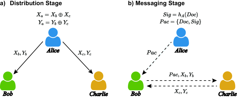
Figure 1: The schematic of the CV QDS protocol. Solid (Dashed) lines represents quantum (classical) channels. The protocol consist of two main parts: distribution stage and messaging stage. a) In the distribution stage, Alice sends optical pulses through quantum channels to Bob and Charlie to generate shared keys in the distribution stage. b) In the messaging stage, Alice generates the signature through OTUH, and sends the packet containing the message and signature to Bob. Bob then sends his keys and received information to Charlie, who will later send his keys to Bob. Bob and Charlie use their own and received keys to infer Alice keys and then perform OTUH test to verify the signature.

In recent years, several CV QDS protocols [49, 50, 51, 52, 53] have been proposed and experimentally demonstrated for signing one-bit message. However, the security of these solutions against general coherent attacks in finite-size regime with quantified failure probabilities remains unproven. The need for theoretical advancement in security proof becomes a major obstacle towards the wide application of CV QDS. A promising route in direction can be adopting some DV techniques in security analysis [54].

In addition to that, extending to multi-bit signature is another challenging task, as simple concatenation without careful coding of single-bit signature can be vulnerable to attacks [55]. To tackle this issue, various approaches have been proposed, primarily involving the encoding of raw messages into new strings and the iterative application of the single-bit protocol to each bit [55, 56, 57, 58, 59]. Ref. [55] encodes each message bit 0(1) into 000(010) and appends a symbol word 111 to both head and tail of the message. Ref. [57] follows a specific coding rule that inserts a bit 0 for every $x$ message bits. Ref. [59] signs each message bit with increasing signature lengths without extra coding. Obviously, these methods sacrifice the signature efficiency in exchange for security and thus their achieved signature rates are low and insufficient for practical implementation.

Fortunately, one-time universal hashing (OTUH) QDS [3] has emerged as a solution to the multi-bit message signing with very high efficiency and unconditional security, containing two key attributes. On the one hand, the users’ secret sharing relationship establishes a strict asymmetry between the signer and the recipient. In this regard, once two recipients collaborate, they will possess identical information (keys), thereby preventing the repudiation attempts by the signer. On the other hand, the use of universal hashing in each update guarantees a strict one-way characteristic, rendering it impossible for the recipient to infer the message from the encrypted hash value. Notably, even with imperfect discrete-variable quantum state [60], where an attacker obtains part of the information, OTUH QDS retains unconditionally secure due to the inherent compression properties of the universal hash functions. Additionally, OTUH QDS with discrete-variable system has been experimentally validated and used to build other quantum protocols [61, 62, 63], such as quantum e-commerce and quantum Byzantine consensus.

In this paper, we present a CV QDS protocol based on the revised OTUH method. As an efficient method which directly signs the hash value of multi-bit messages with just one key string, its application significantly improves the signature efficiency. In addition to that, we adopt discrete-modulated CV approach inspired by a state-of-the-art quantum key distribution work [54] for the generation of shared keys, which guarantees security against general coherent attacks in finite-size regime for the first time. Thanks to the seamlessly integration of both parts, we provide the complete security proof of multi-bit CV QDS scheme. In summary, our protocol efficiently signs multi-bit messages with information-theoretical security, achieving higher signature rates in short distances and requiring inexpensive and readily available apparatus. To demonstrate the superiority of our protocol in performance, we also conduct a numerical simulation under different conditions. From the results, we would find that our protocol can outperform previous CV QDS protocols by over 5 magnitudes in terms of signature rate over a fiber distance of 40 km between the sender and recipient. Furthermore, our protocol is especially good at large-scale signing because the signature rate does not drop dramatically like other CV QDS protocols when message size grows larger. Based on that, potential applications of multi-bit CV QDS can be conceived and outlooked.

The rest of this paper is organized as follows. Sec. II provides an overview of our protocol, detailing the procedures of CV distribution method and the OTUH QDS scheme. In Sec. III, we offer a comprehensive security proof of our protocol, analyzing both the CV procedure and the OTUH method applied in the QDS scheme. Sec. IV showcases numerical simulations conduced to evaluate the performance of our protocol and compare it with previous CV QDS schemes. Lastly, we draw conclusions and engage in a discussion regarding our work in Sec. V.

II Protocol Description

In this section, we first introduce the schematic of our CV QDS protocol. In the simplest instance, we consider a signature scenario involving three parties: one sender, Alice, and two symmetric recipients, Bob and Charlie. Without loss of generality, we assume Bob to be the specified recipient, and Charlie automatically becomes the verifier. For a successful QDS scheme, Bob and Charlie should be able to determine that Alice is the genuine author of $m$, which means the forging and repudiation attacks are prevented. If all participants are honest, the scheme should succeed except with negligible probability.

As shown in Fig. 1, a basic communication network is constructed through quantum (solid lines) and classical (dashed lines) channels. Alice wishes to send a classical $m$-bit message to Bob, which he will forward to Charlie. This scheme could be easily extended to include more participants [64].

The CV QDS protocol comprises two stages: a distribution stage and a messaging stage. In the distribution stage, Alice’s coherent states are measured by Bob and Charlie to generate keys. The key bits possessed by Alice, Bob and Charlie consist of two parts which are $\{X_{a},X_{b},X_{c}\}$ with $n$ bits and $\{Y_{a},Y_{b},Y_{c}\}$ with $2n$ bits respectively, satisfying the perfect correlation conditions $X_{a}=X_{b}\oplus X_{c}$ and $Y_{a}=Y_{b}\oplus Y_{c}$. We remark that the keys are asymmetric for the signer and receiver, i.e. $X_{a}\neq X_{b}$ and $Y_{a}\neq Y_{b}$, which is the prerequisites of the keys’ validity. In the messaging stage, Alice generates the signature $Sig$ with OTUH and transmits the packet $Pac=\{Doc,Sig\}$ containing the message and appended signature generated by shared keys to Bob. Bob then forwards the packet to Charlie along with his keys $\{X_{b},Y_{b}\}$, and Charlie sends his keys $\{X_{c},Y_{c}\}$ in return on receipt. After the exchange, Bob and Charlie verify the integrity and authenticity of the message through a hashing test. The message and signature are accepted if and only if the OTUH tests success on both recipients’ sides. The subsequent contents of this section will elaborate on the procedures of each stage in detail.

II.1 Distribution stage

In the distribution stage, Alice distributes coherent strings as shared keys to Bob and Charlie, respectively, by implementing CV method. To ensure security against general coherent attacks in finite-size regime, a novel fidelity test approach [65, 54] is employed during the parameter estimation process. In upcoming parts, we first introduce this approach and then outline complete steps of the distribution stage.

II.1.1 Fidelity test approach

The core element of our fidelity test approach is a smooth function that maps the unbounded outcome of heterodyne measurement to a bounded value. The smooth function is defined as follows.

Definition 1.

Let $\Lambda_{m,r}(\nu)(\nu\geq 0)$ be the smooth function given by

$$\Lambda_{m,r}(\nu):=e^{-r\nu}(1+r)L_{m}^{(1)}((1+r)\nu)$$ (1)

for an integer $m\geq 0$ and a real number $r>0$. $L^{(k)}_{n}(\nu)$ represents associated Laguerre polynomials given by

$$L_{n}^{(k)}(\nu):=(-1)^{k}\frac{d^{k}L_{n+k}(\nu)}{d\nu^{k}},$$ (2)

where

$$L_{n}(\nu):=\frac{e^{\nu}}{n!}\frac{d^{n}}{d\nu^{n}}\left(e^{-\nu}\nu^{n}\right)$$ (3)

are the Laguerre polynomials. The absolute value and the slope of the function are bounded for small values of $(m,r)$. Here we adopt the optimized value $(m,r)=(1,0.4120)$ to minimize the range of the smooth function.

Based on the definition, we can establish a lower bound on the fidelity of input pulses with a specified confidence level in finite-size regime. For fidelity to a coherent state $|\beta\rangle$, the inequality below holds.

$$\mathbb{E}_{\rho}\left[\Lambda_{m,r}\left(|\hat{\omega}-\beta|^{2}\right)\right]\leq\operatorname{Tr}(\rho|\beta\rangle\langle\beta|)\quad(m:odd).$$ (4)

The proof of this inequality can be found in Appendix A. Upon that, we can obtain a measure of disturbance in the binary modulated CV scheme by monitoring the fidelity. Analogous to the bit errors in the B92 protocol [66, 67, 68], fidelity facilitates the construction of a security proof based on a reduction to entanglement distillation [28, 69], a technique commonly employed in DV schemes.

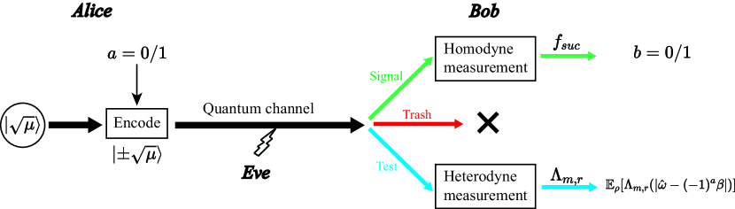
Figure 2: The schematic of key distribution based on CV. Alice generates a random bit $a=0/1$ as her key and uses it to encode a coherent state with amplitude $(-1)^{a}\sqrt{\mu}$. Then she transmit the state to Bob through a quantum channel with potential eavesdroppers Eve and Bob chooses one of the three procedures based on the predetermined probability upon receiving. In the signal round, Bob performs a homodyne measurement with an outcome $\hat{x}$ and use a acceptance function $f_{\text{suc}}$ to obtain his key $b=0/1$. In the test round, he performs a heterodyne measurement with an outcome $\hat{\omega}$ and use the smooth function $\Lambda_{m,r}$ to calculate the bound of fidelity. In the trash round, he produces no outcome.

II.1.2 Steps of key distribution

Because of the symmetry of two recipients, Bob and Charlie, the key distribution procedures are identical between Alice and them respectively. For the simplicity of narration, we take Alice and Bob as example and illustrate the schematic of key distribution in Fig. 2. The detailed procedures are described below.

1. Preparation—Alice generates a random bit $a\in\{0,1\}$ and sends a coherent state with amplitude $(-1)^{a}\sqrt{\mu}$ to Bob. She repeats this process $N$ times.

2. Measurement—For each received optical pulse, Bob chooses a label from $\{$signal, test, trash$\}$ with probabilities $p_{\text{sig}},p_{\text{test}}$ and $p_{\text{trash}}$ respectively. According to the chosen label, Alice and Bob do one of the following procedures.

   signal

   Bob performs a homodyne measurement on the received optical pulse, and obtains an outcome $\hat{x}\in\mathbb{R}$. With a pre-determined probability function $f_{\text{suc}}(|\hat{x}|)$, which is ideally a step function, he regards the detection to be a “success” (otherwise “failure”), and then announces this result of the detection. In the case of a success, he defines a bit b = 0 (1) when $sign(\hat{x})=+(-)$ and keeps $b$ as a sifted key bit which pairs with Alice’s key bit $a$.

   test

   Bob performs a heterodyne measurement on the received optical pulse, and obtains an outcome $\hat{\omega}\in\mathbb{C}$. Alice announces her bit $a$ which makes Bob have the knowledge of the expected amplitude of his received state$(-1)^{a}\beta=(-1)^{a}\sqrt{\eta\mu}$. Here $\eta$ is the nominal transmissivity of the quantum channel between Alice and Bob. Then Bob calculates the value of $\Lambda_{m,r}(|\hat{\omega}-(-1)^{a}\beta|^{2})$.

   trash

   Alice and Bob produce no outcomes.

   We refer to the numbers of “success” and “failure” signal rounds, test rounds, and trash rounds as $\hat{N}^{\text{suc}},\hat{N}^{\text{fail}},\hat{N}^{\text{test}}$ and $\hat{N}^{\text{trash}}$, respectively ($N=\hat{N}^{\text{suc}}+\hat{N}^{\text{fail}}+\hat{N}^{\text{test}}+\hat{N}^{\text{trash}}$ holds by definition).

3. Parameter estimation—Bob calculates the sum of $\Lambda_{m,r}(|\hat{\omega}-(-1)^{a}\beta|^{2})$ obtained in the $\hat{N}^{\text{test}}$ test rounds for the fidelity test, which is denoted by $\hat{F}$. For the bit error rate, Alice and Bob compare several bits to estimate.

4. Error correction—Alice and Bob consume part of keys through encrypted communication to perform following actions. Alice communicates Bob through linear codes for her sifted key and Bob reconciles his sifted key accordingly. We denote $H$ as the binary Shannon entropy, and then the consumption of this process can be estimated by $fH(E^{b})\hat{N}^{\text{suc}}$ according to information theory, where $f$ is the error correction efficiency and $E^{b}$ represents the bit error rate of raw keys. Alice and Bob then verify the correction by comparing $\log_{2}{(1/{\epsilon_{\text{cor}}})}$ bits via universal hashing. Here $\epsilon_{\text{cor}}$ is the failure probability of this error correction process. The number of final keys is thus given by

   $$\hat{N}^{\text{fin}}=\hat{N}^{\text{suc}}[1-fH(E^{b})]-\log_{2}{\frac{1}{\epsilon_{\text{cor}}}}.$$ (5)

5. Examination of unknown information—For the distilled $\hat{N}^{\text{fin}}$-bit keys, Alice then disrupts the orders of them randomly and publicizes the new order to Bob through the authenticated channel. Subsequently, Alice and Bob divide the final keys into several $n$-bit group, each of which is used for a signature task during the messaging stage. This procedure ensures that the attacker cannot predict the position of each bit within a specific group in advance. Therefore, the grouping process can be viewed as a form of random sampling in our finite-size analysis. The maximum unknown information of an $n$-bit group available to the attacker after error correction $\mathcal{H}_{n}$ can be estimated by

   $$\mathcal{H}_{n}\leq n[1-H(E^{\phi n})].$$ (6)

   Here, $E^{\phi n}$ is the upper bound of the phase error rate in each $n$-bit group which can be calculated based on the estimated phase error rate of final keys $E^{\phi}$ and group size $n$. The detailed expression for this calculation can be found in Appendix B.1.

Furthermore, it is worth noting that we omit the privacy amplification process, which is commonly employed in quantum communication. This omission is attributed to the specific utilization and requirements of distributed keys in QDS schemes. Recently Ref. [60] has proved that keys with full correctness and imperfect secrecy are capable of realizing secure QDS protocols. We adopt this technique and estimate specific parameters of final keys for further calculations in subsequent section of this article.

II.2 Messaging stage

In the messaging stage, we adopt the OTUH method which leverages the almost XOR universal (AXU) hash function to generate the signature for a long message. For the clarity of narration, we first introduce the AXU hash function and its properties.

II.2.1 AXU hash function

The AXU hash function is a special class of hash functions that map input values of arbitrary length to almost random hash values with a fixed length [70]. The signature generated in OTUH QDS corresponds to the AXU hash value of the message to be signed, with the AXU hash function be determined by just one string of Alice keys.

Various AXU hash can be employed in the messaging stage of our protocol depending on the diverse application scenarios of users. To demonstrate the messaging procedures in detail, we choose the linear feedback shift register-based (LFSR-based) Toeplitz hashing method [71] as our hash function.

Definition 2.

LFSR-based Toeplitz hash function: LFSR-based Toeplitz hash function can be expressed as $h_{p,s}(M)=H_{nm}\cdot M$ , where $p,s$ determines the function and $M$ is the message in the form of an $m$-bit vector. The detailed process of generating LFSR-based Toeplitz hash function is as follows. A randomly selected irreducible polynomial of order $n$ in the field GF(2), $p(x)$, determines the construction of LFSR. $p(x)=x^{n}+p_{n-1}x^{n-1}+\dots+p_{1}x+p_{0}$ can be characterized by its coefficients of order from 0 to $n-1$, i.e., $p_{a}=(p^{n-1},p_{n-2},\dots,p_{1},p_{0})$. For the initial state $s$ which is also represented as an $n$-bit vector $s=(a_{n},a_{n-1},\dots,a_{2},a_{1})^{T}$, the LFSR will be performed $m$ times to generate $m$ vectors. Specifically, it will shift down every element in the previous column, and add a new element to the top of the column. For example, the LFSR transforms $s$ into $s_{1}=(a_{n+1},a_{n},\dots,a_{3},a_{2})^{T}$, where $a_{n+1}=p_{a}\cdot s$, and likewise, transforms $s_{1}$ to $s_{2}$. Then the $m$ vectors $s,s_{1},\dots,s_{m-1}$ will together construct the Toeplitz matrix $H_{nm}=(s,s_{1},\dots,s_{m-1})$, and the hash value of the massage is $H_{nm}\cdot M$.

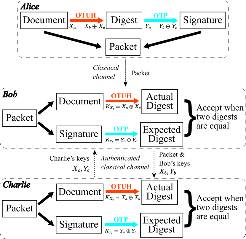
Figure 3: The schematic of OTUH QDS applied in the messaging stage. The OTUH (orange arrow) and OTP (blue arrow) method constitutes core steps in our QDS scheme to encode (Alice) and decode (Bob and Charlie) digest and signature, which guarantee the information-theoretical security of the protocol.

II.2.2 Steps of messaging

The schematic of OTUH QDS is shown is Fig. 3, we then describe steps adopting this method in messaging stage in detail.

1. Signing of Alice—First, Alice uses a local quantum random number, characterized by an $n$-bit string $p_{a}$, to randomly generate an irreducible polynomial $p(x)$ of degree $n$ [1]. Second, she uses the initial vector (key bit string $X_{a}$) and irreducible polynomial (quantum random number $p_{a}$) to generate a random LFSR-based Toeplitz matrix $H_{nm}$, with $n$ rows and $m$ columns. Third, she uses a hash operation with $Hash=H_{nm}\cdot Doc$ to acquire an $n$-bit hash value of the $m$-bit document. Fourth, she exploits the hash value and the irreducible polynomial to constitute the $2n$-bit digest $Dig=(Hash||p_{a})$. Fifth, she encrypts the digest with her key bit string $Y_{a}$ to obtain the $2n$-bit signature $Sig=Dig\oplus Y_{a}$ using OTP. Finally, she uses the public channel to send the message packet containing the signature and document $Pac=\{Sig,Doc\}$ to Bob.

2. Verification of Bob—Bob uses the authentication classical channel to transmit the received $Pac$, as well as his key bit strings $\{X_{b},Y_{b}\}$, to Charlie. Then, Charlie uses the same authentication channel to forward his key bit strings $\{X_{c},Y_{c}\}$ to Bob. Bob obtains two new key bit strings $\{K_{X_{b}}=X_{b}\oplus X_{c},K_{Y_{b}}=Y_{b}\oplus Y_{c}\}$ by the XOR operation. Bob exploits $K_{Y_{b}}$ to obtain an expected digest and bit string $p_{b}$ via XOR decryption. Bob utilizes the initial vector $K_{X_{b}}$ and irreducible polynomial $p_{b}$ to establish an LFSR-based Toeplitz matrix. He uses a hash operation to acquire an n-bit hash value and then constitutes a $2n$-bit actual digest. Bob will accept the signature if the actual digest is equal to the expected. Then, he informs Charlie of the result. Otherwise, Bob rejects the signature and announces to abort the protocol.

3. Verification of Charlie—If Bob announces that he accepts the signature, Charlie then uses his original key and the key sent to Bob to create two new key bit strings $\{K_{X_{c}}=X_{b}\oplus X_{c},K_{Y_{c}}=Y_{b}\oplus Y_{c}\}$. Charlie employs $K_{Y_{c}}$ to acquire an expected digest and bit string $p_{c}$ via XOR decryption. Charlie uses a hash operation to obtain an $n$-bit hash value and then constitutes a $2n$-bit actual digest, where the hash function is generated by initial vector $K_{X_{c}}$ and irreducible polynomial $p_{c}$. Charlie accepts the signature if the two digests are identical. Otherwise, Charlie rejects the signature.

For the scheme with LFSR based Toeplitz hashing, a message of length $M$ requires Alice to generate six bit strings $X_{b},X_{c},Y_{b},Y_{c},Z_{b},Z_{c}$, each of length $n$. Thus the signature rate is

$$R=G/3n.$$ (7)

III Security Analysis

In order to establish the security proof of our protocol, it is imperative to estimate certain security parameters related to the shared keys during the distribution stage. Drawing inspiration from Ref. [54], a novel technique can be employed to estimate the bit error rate and phase error rate of final keys. In subsequent contents, we will first focus on the estimation technique in finite-size scenario and then utilize estimated parameters to conduct a comprehensive security analysis of our protocol.

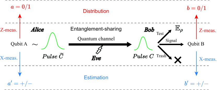
Figure 4: Relation between estimation and distribution procedures. The estimation (blue) and distribution (red) procedures are related through their common entanglement-sharing part. After the entanglement-sharing part, Alice and Bob are left with the observed data $(\hat{N}^{\text{suc}},\hat{N}^{\text{fail}},\hat{N}^{\text{test}},\hat{N}^{\text{trash}},\hat{F},\hat{Q}_{-})$ and $\hat{N}^{\text{suc}}$ pairs of qubits. If Alice and Bob ignore $\hat{Q}_{-}$ and measure their qubits on the $Z$-basis to determine their $\hat{N}^{\text{suc}}$-bit sifted keys, it becomes equivalent to the actual distribution procedure. On the other hand, if Alice and Bob measure their qubits on the $X$-basis, they can count the number of phase error $\hat{N}^{\text{suc}}_{\text{ph}}$, which we call the estimation procedure. If we can find an upper bound $U$ on $\hat{N}^{\text{suc}}_{\text{ph}}$, it restricts the property of $\hat{N}^{\text{suc}}$ pairs of qubits after entanglement-sharing, which in turn limits the leaked information on the sifted keys in the actual distribution procedure. Thus the security proof is reduced to finding a proper upper bound $U$ represented as a function of the variables that are commonly available in two procedures.

III.1 Security of CV method

III.1.1 Entanglement based description

The Shor-Preskill method [28, 72], widely used in DV protocols, is introduced here as the foundation of our analysis. First we consider a coherent version of Step 1 and 2 in the distribution stage, where Alice and Bob share an entangled pair of qubits for each success signal round. Following that, their $Z$-basis measurement outcomes would correspond to the sifted key bits $a$ and $b$. Alice possesses a qubit $A$, which she entangles with an optical pulse $\tilde{C}$ in a state

$$|\Psi\rangle_{A\tilde{C}}:=\frac{|0\rangle_{A}|\sqrt{\mu}\rangle_{\tilde{C}}+|1\rangle_{A}|-\sqrt{\mu}\rangle_{\tilde{C}}}{\sqrt{2}}.$$ (8)

Then, Step 1 is equivalent to the preparation of $|\Psi\rangle_{A\tilde{C}}$ followed by a measurement of the qubit $A$ on $Z$ basis $\{|0\rangle,|1\rangle\}$ to determine the bit value $a$. For Bob, he probabilistically converts the received optical pulse $C$ to a qubit $B$. This process can be described as a completely positive (CP) map defined by

$$\mathcal{F}_{C\rightarrow B}\left(\rho_{C}\right):=\int_{0}^{\infty}dxK^{(x)}\rho_{C}K^{(x)\dagger}$$ (9)

with

$$K^{(x)}:=\sqrt{f_{\text{suc}}(x)}(|0\rangle_{B}\langle x|_{C}+|1\rangle_{B}\langle-x|_{C}),$$ (10)

where $\langle x|$ maps a state vector to the value of its wave function at $x$. We assume that the pulse $C$ is in a state $\rho_{C}$ and the corresponding process succeeds with a probability $p_{\text{suc}}$, then the relation $p_{\text{suc}}\rho_{B}=\mathcal{F}_{C\rightarrow B}(\rho_{C})$ holds for the qubit $B$ in a state $\rho_{B}$. If the qubit $B$ is further measured on $Z$ basis , probabilities of the outcome $b=0,1$ are given by

$$p_{\text{suc}}\langle 0|\rho_{B}|0\rangle=\int_{0}^{\infty}f_{\text{suc }}(x)dx\langle x|\rho_{C}|x\rangle,$$ (11)

$$p_{\text{suc}}\langle 1|\rho_{B}|1\rangle=\int_{0}^{\infty}f_{\text{suc}}(x)dx\langle-x|\rho_{C}|-x\rangle,$$ (12)

which shows the equivalence to the signal round in Step 2. As a result, above procedures are equivalent to Steps 1 through 2 of the distribution stage for Alice and Bob to share sifted keys.

For the parameter estimation task, we need to focus on the phase error rate of sifted keys which is directly connected to the amount of privacy amplification. Suppose that, after the preparation of qubit $B$ mentioned above, Alice and Bob measure their $\hat{N}^{\text{suc}}$ pairs of qubits on $X$ basis $\{|+\rangle,|-\rangle\}$ instead of $Z$ basis $\{|0\rangle,|1\rangle\}$, it is obvious that a pair with outcomes $(+,-)$ or $(-,+)$ is defined to be the phase error. Then we can record the number of phase errors denoted by $\hat{N}^{\text{suc}}_{\text{ph}}$ among $\hat{N}^{\text{suc}}$ pairs. Here our target is to acquire a good upper bound $e_{\text{ph}}$ on the phase error rate $\hat{N}^{\text{suc}}_{\text{ph}}/\hat{N}^{\text{suc}}$, the binary Shannon entropy $h(e_{\text{ph}})$ of which is the sufficient consumption for privacy amplification in the asymptotic limit.

To tackle the finite-size case as well, we necessitate a more rigorous upper bound analysis of phase error rate. Consequently, we introduce an estimation protocol that not only validates above observation but also demonstrates the fundamental principles of our proof technique in the following part.

III.1.2 Estimation protocol

1. Preparation—Alice prepares a qubit $A$ and an optical pulse $\tilde{C}$ in an entangled state $|\Psi\rangle_{A\widetilde{C}}$ defined in Eq. (8). She repeats it $N$ times.

2. Measurement—For each received pulse, Bob announces a label in the same way as that in Step 2. According to the chosen label, Alice and Bob do one of the following procedures.

   signal

   Bob performs a quantum operation on the received pulse $C$ specified by the CP map $\mathcal{F}_{C\rightarrow B}$ to determine success/failure of the detection and obtain a qubit $B$ upon success. He announces success/failure of detection. In the case of a success, Alice keeps her qubit $A$.

   test

   Bob performs a heterodyne measurement on the received optical pulse $C$, and obtains an outcome $\hat{\omega}$. Alice measures her qubit $A$ on $Z$ basis and announces the outcome $a\in\{0,1\}$. Bob calculates the value of $\Lambda_{m,r}(|\hat{\omega}-(-1)^{a}\beta|^{2})$ as defined in Step 2.

   trash

   Alice measures her qubit $A$ on $X$ basis to obtain $a^{\prime}\in\{+,-\}$.

   Here $\hat{N}^{\text{suc}},\hat{N}^{\text{fail}},\hat{N}^{\text{test}},\hat{N}^{\text{trash}}$ and $\hat{F}$ are defined in the same way as those in Step 2. Let $\hat{Q}_{-}$ be the number of rounds in the $\hat{N}^{\text{trash}}$ trash rounds with $a^{\prime}=-$.

3. Parameter Estimation—Alice and Bob measure each of their $\hat{N}^{\text{suc}}$ pairs of qubits on $X$ basis and obtain outcomes $a^{\prime\prime}$ and $b^{\prime\prime}$, respectively. Let $\hat{N}^{\text{suc}}_{\text{ph}}$ be the number of pairs found in the combination $(a^{\prime\prime},b^{\prime\prime})=(+,-)$ or $(-,+)$.

After such definition, the task of proving the security of the actual protocol is then reduced to construction of a function $U(\hat{F},\hat{N}^{\text{trash}})$ which satisfies

$$\operatorname{Pr}\left[\hat{N}_{\mathrm{ph}}^{\mathrm{suc}}\leq U\left(\hat{F},\hat{N}^{\text{trash }}\right)\right]\geq 1-\epsilon$$ (13)

for any attack towards the estimation protocol in finite-size regime. Here the parameter $\epsilon$ are security parameter chosen by us. In recent work, it has been shown that the condition above immediately implies the security for the actual distribution stage. The detailed definition and proof of security can be found in Ref. [73, 72, 74].

Next, we should make some clarification about what property of the optical pulse $C$ Bob could get through his $X$-basis measurement in this estimation protocol. Let $\Pi_{\text{ev(od)}}$ be a projection operator to the subspace with even (odd) photon numbers. ($\Pi_{\text{ev}}+\Pi_{\text{od}}=\mathbb{I}_{C}$ holds by definition.) There is simple property that $\Pi_{\text{ev}}-\Pi_{\text{od}}$ is the operator for an optical phase shift of $\pi$, so we have $(\Pi_{\text{ev}}-\Pi_{\text{od}})|x\rangle=|-x\rangle$. Then Eq. (10) can be rewritten as

$$K^{(x)}=\sqrt{2f_{\mathrm{suc}}(x)}(|+\rangle_{B}\langle x|_{C}\Pi_{\mathrm{ev}}+\mid-\rangle_{B}\langle x|_{C}\Pi_{\mathrm{od}}).$$ (14)

Therefore, when the state of the pulse $C$ is $\rho_{C}$, the probability of obtaining $+(-)$ in the $X$-basis measurement in the estimation protocol is given by

$$\left\langle+(-)\left|\mathcal{F}_{C\rightarrow B}\left(\rho_{C}\right)\right|+(-)\right\rangle=\operatorname{Tr}\left(\rho_{C}M_{\mathrm{ev}(\mathrm{od})}^{\mathrm{suc}}\right),$$ (15)

where

$$M_{\mathrm{ev}(\mathrm{od})}^{\mathrm{suc}}:=\int_{0}^{\infty}2f_{\mathrm{suc}}(x)dx\Pi_{\mathrm{ev}(\mathrm{od})}|x\rangle\langle x|_{C}\Pi_{\mathrm{ev}(\mathrm{od})}.$$ (16)

This equation means that the sign of Bob’s $X$-basis measurement outcome distinguishes the parity of the photon number of the received pulse, such that the secrecy of our protocol is assured by the complementarity between these two characteristics.

III.1.3 Upper bound of phase error rate

As an intermediate step toward our final goal of condition (13), let us first derive a bound on the expectation value $\mathbb{E}[\hat{N}^{\text{suc}}_{\text{ph}}]$ in terms of those collected in the test and the trash rounds, $\mathbb{E}[\hat{F}]$ and $\mathbb{E}[\hat{Q}_{-}]$, in the estimation protocol. We define relevant operators as

$$M_{\mathrm{ph}}^{\mathrm{suc}}:=|+\rangle\langle+|_{A}\otimes M_{\mathrm{od}}^{\mathrm{suc}}+\mid-\rangle\langle-|_{A}\otimes M_{\mathrm{ev}}^{\mathrm{suc}},$$ (17)

$$\Pi^{\mathrm{fid}}:=|0\rangle\langle 0|_{A}\otimes\beta\rangle\langle\beta|_{C}+1\rangle\langle 1|_{A}\otimes-\beta\rangle\langle-\beta|_{C},$$ (18)

$$\Pi_{-}^{\text{trash }}:=|-\rangle\langle-|_{A}\otimes\mathbb{I}_{C}.$$ (19)

Then we immediately have

$$\mathbb{E}[\hat{N}_{\mathrm{ph}}^{\mathrm{suc}}]=p_{\mathrm{sig}}N\operatorname{Tr}(\rho_{AC}M_{\mathrm{ph}}^{\mathrm{suc}}),$$ (20)

$$\mathbb{E}[\hat{F}]\leq p_{\text{test }}N\operatorname{Tr}(\rho_{AC}\Pi^{\text{fid}}),$$ (21)

$$\mathbb{E}[\hat{Q}_{-}]=p_{\text{trash}}N\operatorname{Tr}(\rho_{AC}\Pi_{-}^{\text{trash }}).$$ (22)

Here we apply Eq. (4) to derive the inequality above. For simplicity, we denote $\operatorname{Tr}(\rho_{AC}M)$ as $\langle M\rangle$ for any operator $M$. The set of points $(\langle M^{\text{suc}}_{\text{ph}}\rangle,\langle\Pi^{\text{fid}}\rangle,\langle\Pi^{\text{trash}}_{-}\rangle)$ for all the density operators $\rho_{AC}$ form a convex region. Rather than directly deriving the boundary of the region, it is easier to pursue linear constraints in the form of

$$\left\langle M_{\mathrm{ph}}^{\mathrm{suc}}\right\rangle\leq B(\kappa,\gamma)-\kappa\left\langle\Pi^{\mathrm{fid}}\right\rangle+\gamma\left\langle\Pi_{-}^{\mathrm{trash}}\right\rangle,$$ (23)

where $B(\kappa,\gamma),\kappa,\gamma\in\mathbb{R}$. It is expected that a meaningful bound is obtained only for $\kappa,\gamma\geq 0$, because decreasing fidelity $\left\langle\Pi^{\mathrm{fid}}\right\rangle$ and stronger pulse, which directly increases $\left\langle\Pi_{-}^{\mathrm{trash}}\right\rangle$, would lead to a larger value of phase error rate.

To find a function $B(\kappa,\gamma)$ satisfying Eq. (23), let us define an operator

$$M[\kappa,\gamma]:=M_{\mathrm{ph}}^{\mathrm{suc}}+\kappa\Pi^{\mathrm{fid}}-\gamma\Pi_{-}^{\mathrm{trash}}.$$ (24)

Then Eq. (23) is rewritten as $\operatorname{Tr}(\rho_{AC}M[\kappa,\gamma])\leq B(\kappa,\gamma)$. This condition should hold for all $\rho_{AC}$ iff $M[\kappa,\gamma]$ satisfies an operator inequality

$$M[\kappa,\gamma]\leq B(\kappa,\gamma)\mathbb{I}_{AC}.$$ (25)

Theoretically speaking, although $B(\kappa,\gamma)=\sigma_{\text{sup}}(M[\kappa,\gamma])$ would give the tightest bound for the operator inequality above, where $\sigma_{\text{sup}}(O)$ denotes the supremum of the spectrum of a bounded self-adjoint operator $O$(i.e. the maximum modulus of eigenvalues of a matrix), it is difficult to compute it numerically since $M[\kappa,\gamma]$ has an infinite rank. As a compromise for the computable but not necessarily tight bound, we reduce the problem to replacing $M[\kappa,\gamma]$ with a constant upper bound except in a relevant finite-dimensional subspace spanned by $|\pm\beta\rangle$ and $M^{\text{suc}}_{\text{ev(od)}}|\pm\beta\rangle$. Then we just need to calculate the eigenvalues of some small-size matrices to get $B(\kappa,\gamma)$. For the detailed expression of $B(\kappa,\gamma)$, see Appendix B.2.

With $B(\kappa,\gamma)$ computed, we can rewrite Eq. (23) to obtain

$$\mathbb{E}[\hat{T}[\kappa,\gamma]]\leq NB(\kappa,\gamma),$$ (26)

where $\hat{T}[\kappa,\gamma]:=p_{\text{sig }}^{-1}\hat{N}_{\mathrm{ph}}^{\mathrm{suc}}+p_{\text{test }}^{-1}\kappa\hat{F}-p_{\text{trash }}^{-1}\gamma\hat{Q}_{-}$. This relation directly leads to an explicit bound on the phase error rate as

$$\mathbb{E}\left[\hat{N}_{\mathrm{ph}}^{\mathrm{suc}}\right]/p_{\mathrm{sig}}N\leq B(\kappa,\gamma)+\gamma q_{-}-\kappa\mathbb{E}[\hat{F}]/p_{\text{test }}N,$$ (27)

which is enough for the computation of asymptotic key rates. Here $q_{-}$ is short for $\mathbb{E}[\hat{Q}_{-}]$.

As for the finite-size regime, the proof could be provided as follows. We use Azuma’s inequality [75] to evaluate the fluctuations around the expectation value, leading to an inequality revised from Eq. (26)

$$\hat{T}[\kappa,\gamma]\leq NB(\kappa,\gamma)+\delta_{1}(\epsilon/2),$$ (28)

which holds with a probability no smaller than $1-\epsilon/2$ (see Appendix B.3 for detailed expression of function $\delta_{1}$).

Another revision of proof happens in the definition of $\hat{T}[\kappa,\gamma]$. It includes $\hat{Q}_{-}$ which is inaccessible in the actual distribution stage, but we can derive bound by noticing that it is an outcome from Alice’s qubits and independent of the adversary’s attack. In fact, given $\hat{N}_{\text{trash}}$, it is the tally of $\hat{N}_{\text{trash}}$ Bernoulli trials with a probability $q_{-}$. Hence, we can derive an inequality of the form

$$\hat{Q}_{-}\leq q_{-}\hat{N}^{\text{trash }}+\delta_{2}\left(\epsilon/2;\hat{N}^{\text{trash }}\right),$$ (29)

which holds with a probability no smaller than $1-\epsilon/2$. Here $\delta_{2}(\epsilon/2;\hat{N}^{\text{trash}})$ can be determined by a Chernoff bound (see Appendix B.3 for detailed expression of function $\delta_{2}$). Combining Eq. (28) and (29), we obtain $U(\hat{F},\hat{N}^{\text{trash}})$ satisfying Eq. (13) as

$$U(\hat{F},\hat{N}^{\text{trash }}):= p_{\text{sig }}NB(\kappa,\gamma)+p_{\text{sig }}\delta_{1}(\epsilon/2)-\frac{p_{\text{sig }}}{p_{\text{test }}}\kappa\hat{F}$$ (30)

$$+\frac{p_{\text{sig }}}{p_{\text{trash }}}\gamma(q_{-}\hat{N}^{\text{trash }}+\delta_{2}(\epsilon/2;\hat{N}^{\text{trash }})),$$

which completes our security proof in finite-size regime.

III.2 Security of QDS

In this part, we first focus on the properties of AXU hashing in the context of imperfect keys with limited secrecy leakage and then discuss the security of the entire QDS system.

III.2.1 Attacks on AXU hashing

There are various attacks available for the attacker to perform towards the AXU hashing method. The worst strategy is to randomly generate $m,t$ to satisfy $h_{p,s}(m)=t$, whose success probability is only $2^{-n}$. We will leave out this attack in the following analysis. Apart from this, remaining attacks includes guessing keys and recovering keys from signatures. For the latter strategy, as the signature is encrypted by the key strings, the attacker must guess the key strings before the recovering algorithm. This will reduce its success probability to no more than that of just guessing keys. Therefore, the optimal strategy on AXU hashing is to directly guess the key string that encrypts the polynomial. In the following paragraphs, we will focus on bounding the success probability of this strategy.

Firstly, we quantify the guessing probability of the attacker when he is to guess an $n$-bit key string with limited secrecy leakage. Suppose the $n$-bit key string is $X$ and the attacker’s system is $B$, the general attack is modeled as a process where attackers can perform any operations on the system of all quantum states, get a system $\rho_{B}^{x}$ and perform any positive operator-valued measure $\{E_{B}^{x}\}_{x}$ performed on it. The probability that the attacker correctly guesses $X$ when in optimal situation is denoted as $P_{\text{guess}}(X|B)$. According to the definition of min-entropy [76], it naturally leads to

$$P_{\text{guess }}(X|B)=\max_{\left\{E_{B}^{x}\right\}_{x}}\sum_{x}P_{x}\operatorname{tr}\left(E_{B}^{x}\rho_{B}^{x}\right)=2^{-H_{\min}(X\mid B)_{\rho}},$$ (31)

where $H_{\min}(X|B)_{\rho}$ is the min-entropy of $X$ and $B$. If $X$ is generated in the distribution stage of our protocol, the min-entropy can be further estimated by $H_{\min}(X|B)_{\rho}=\mathcal{H}_{n}$.

Next, we provide detailed analysis about the LFSR-based Toeplitz hash function (see Definition 2) used in our protocol. Despite the utilization of two different keys, $X_{a}$ and $Y_{a}$, in the hash function, we could show that only guessing $X_{a}$ is enough to perform an effective attack. Suppose the attacker obtains a string $X_{g}$ as his estimation of $X_{a}$. He can decrypt it to obtain $p_{g}$ as his guessing of $p_{a}$ and transform $p_{g}$ into a polynomial $p_{g}(x)$ with $n$-order. If a $m$-bit string $g$ and its matching polynomial $g(x)$ is generated to satisfy $p_{g}(x)|g(x)$, it can be proved (see Appendix. C) that there is the relationship $h(g)=0$ if $p_{g}=p_{a}$ (or equivalently $X_{g}=X_{a}$). This construction is simple since the attacker can select no more than $m/n$ polynomials and multiply them to constitute his choice of $g(x)$ with $m$-order, which means he would guess the string $X_{a}$ for no more than $m/n$ times. Additionally, it must be noted that the attacker knows $p_{a}$ is irreducible, so he will only choose those guesses that satisfy this condition. The success probability of this optimized strategy can be expressed as

$$P_{1}=\frac{m}{n}\cdot P\left(X_{a}=X_{g}\mid p_{g}\in\mathcal{I}\right),$$ (32)

where $P(A|B)$ represents conditional probability and $\mathcal{I}$ is the set of all irreducible polynomials of order $n$ in GF(2). The cardinal number of $\mathcal{I}$, i.e., the number of all irreducible polynomials of order $n$ in GF(2), is more than $2^{n-1}/n$. Thus $P(p_{g}\in\mathcal{I})\leq(2^{n-1}/n)/2^{n}=1/2n$. It is obvious that $P(X_{a}=X_{g},p_{g}\in\mathcal{I})=P(X_{a}=X_{g})$ as $X_{a}=X_{g}$ assures $p_{g}=p_{a}\in\mathcal{I}$. Finally, we can get the estimation of the success probability of this kind of attack.

$$P_{1} =\frac{m}{n}\cdot\frac{P\left(X_{a}=X_{g}\right)}{P\left(p_{g}\in\mathcal{I}\right)}$$ (33)

$$\leq\frac{m}{n}\cdot\frac{2^{-\mathcal{H}_{n}}}{\frac{1}{2n}}=m\cdot 2^{1-\mathcal{H}_{n}}$$

We denote the quantified upper bound above as $\epsilon_{\mathrm{LFSR}}$. In other words, it bounds the failure probability of authentication based on LFSR-based Toeplitz hashing with imperfect keys, given as

$$\epsilon_{\mathrm{LFSR}}=m\cdot 2^{1-\mathcal{H}_{n}}$$ (34)

III.2.2 Security of QDS scheme

In a QDS scheme, the security analysis contains three parts: robustness, non-repudiation and unforgeability.

1. Robustness—The abortion in an honest run occurs only when Alice and Bob (or Charlie) share different key strings after the distribution stage. In our protocol, Alice and Bob (Charlie) will perform error correction in the distribution stage, which makes them share the identical final key. Thus, the robustness bound is $\epsilon_{\mathrm{rob}}=2\epsilon_{\mathrm{cor}}+2\epsilon^{\prime}$, where $\epsilon_{\mathrm{cor}}$ is the failure probability of error correction and $\epsilon^{\prime}$ is the probability that error occurs in classical message transmission. Here we assume $\epsilon^{\prime}=10^{-11}$ for simplicity.

2. Non-repudiation—Alice successfully repudiates when Bob accepts the message while Charlie rejects it. For Alice’s repudiation attacks, Bob and Charlie should be both honest. From the perspective of Alice, Bob and Charlie’s keys are totally symmetric and would lead to the same decision for the same message and signature. Thus, Alice’s repudiation attack succeed only when error occurs in one of the key exchange steps, i.e., the repudiation bound is $\epsilon_{\mathrm{rep}}=2\epsilon^{\prime}$.

   

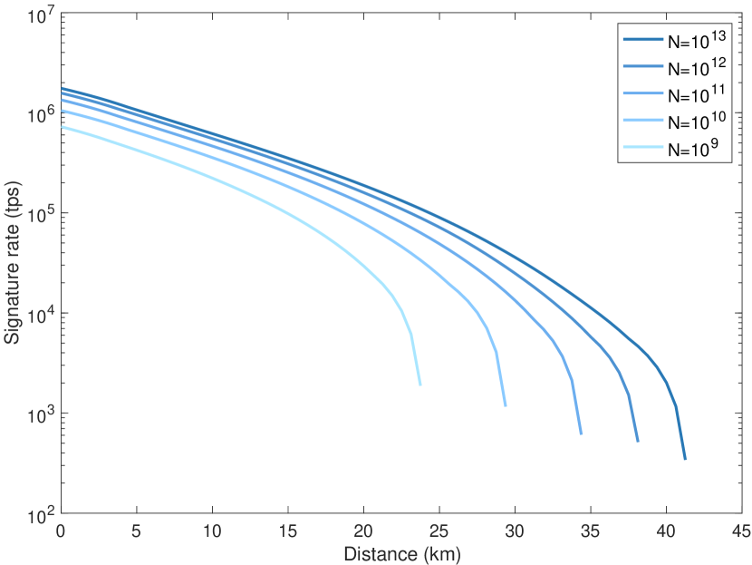
   Figure 5: Signature rates of our protocol under different data sizes $10^{13},10^{12},10^{11},10^{10}$ and $10^{9}$. The amount of excess noise is set to $0$. The message size is assumed to be 1 Kb and the repetition rate of the laser is 1 GHz. The security bound is $10^{-10}$

   

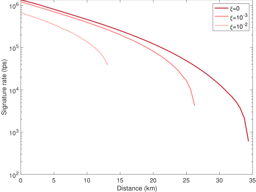
   Figure 6: Signature rates of our protocol with different amount of excess noise $\xi=0,10^{-3}$ and $10^{-2}$. The data size is $10^{11}$. The message size is assumed to be 1 Kb and the repetition rate of the laser is 1 GHz. The security bound is $10^{-10}$

3. Unforgeability—Bob forges successfully when Charlie accepts the forged message forwarded by Bob. After distribution stage, Bob (Charlie) can obtain no information of Alice’s keys which decides the AXU hash function before he transfer the message and signature to Charlie (Bob). Then Bob’s (Charlie’s) forging attack in this protocol is equivalent to the attack attempting to forge the authenticated information sent from Alice to Charlie. Therefore, the probability of a successful forgery can be determined by the failure probability of hashing, i.e., one chooses two distinct messages with identical hash values. For the scheme utilizing LFSR-based Toeplitz hash , the bound is $\epsilon_{\mathrm{for}}=m\cdot 2^{1-\mathcal{H}_{n}}$.

In conclusion, the total security bound of QDS, i.e., the maximum failure probability of the protocol, is $\epsilon=\max\{\epsilon_{\mathrm{rob}},\epsilon_{\mathrm{rep}},\epsilon_{\mathrm{for}}\}$.

IV Results

To demonstrate the performance of our protocol, we build a simulation to calculate the signature rate with different parameters. To begin with, we introduce the simulation model for our numerical calculation.

IV.1 Numerical simulation

We assume a channel model with a loss with transmissivity $\eta$ and an excess noise $\xi$ at channel output. The expected amplitude of coherent state $\beta$ is chosen to be $\sqrt{\eta\mu}$. The states Bob received are obtained by randomly displacing coherent states $|\pm\eta\mu\rangle$ to increase their variances by a factor of $(1+\xi)$. The repetition rate of the laser is 1 GHz and the distances between Alice-Bob and Alice-Charlie are assumed to be the same. We assume a step function with a threshold $x_{\text{th}}(>0)$ as the acceptance probability $f_{\text{suc}}(|x|)$. For the fidelity test, we adopted $m=1$ and $r=0.4120$, which leads to $(\max\Lambda_{m,r},\min\Lambda_{m,r})=(2.824,-0.9932)$. We take parameters $\epsilon_{\text{cor}}=2^{-51}$ and $\epsilon=2^{-104}$. The security bound for calculation is set to $10^{-10}$.

Under these preliminary settings, we thus have two coefficients $(\kappa,\gamma)$ and five protocol parameters $(\mu,x_{\text{th}},p_{\text{sig}},p_{\text{test}},n)$ to be determined. For each transmissivity $\eta$ and excess noise $\xi$, we calculate $(\kappa,\gamma)$ via convex optimization using the CVXR package and $(\mu,x_{\text{th}},p_{\text{sig}},p_{\text{test}})$ via Genetic Algorithm (GA) function in MATLAB, in order to maximize the number of final key in distribution stage. After such operation, we search for the minimal value of signature group size $n$ so that $\epsilon_{\mathrm{LFSR}}$ satisfies the QDS security bound which is set to be $10^{-10}$ using the bit and phase error rate calculated in distribution stage. Typical optimized values of the threshold $x_{\text{th}}$ range from 0.4 to 1.5 (we adopted a normalization for which the vacuum variance is $V=0.25$). See Appendix D for more detailed equations for our numerical simulation.

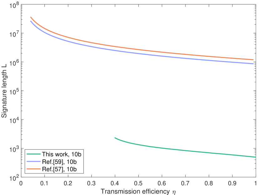
Figure 7: Signature length $L$ required to sign 10b message in our protocol, Ref. [57] and Ref. [59] against transmission efficiency $\eta$. The distances between Alice-Bob and Alice-Charlie are assumed to be the same. The data size N is $10^{11}$ and excess noise is $\xi=10^{-3}$. The security bound is $10^{-10}$.

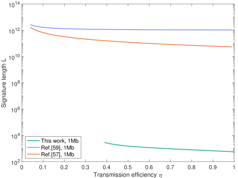
Figure 8: Signature length $L$ required to sign 1Mb message in our protocol, Ref. [57] and Ref. [59] against transmission efficiency $\eta$. The distances between Alice-Bob and Alice-Charlie are assumed to be the same. The data size N is $10^{11}$ and excess noise is $\xi=10^{-3}$. The security bound is $10^{-10}$.

Fig. 6 and 6 show the simulated signature rates of our protocol in finite-size cases $N=10^{9}-10^{13}$ with excess noise $\xi=0,10^{-3},10^{-2}$. In the optimal case, our protocol conduct $10^{6}$ turns of signing task per second in optimal case and reach a transmission distance of over 40km with considerable signature rate. In Fig. 6, we show the performance of our protocol under different data sizes $N$. Even with a data size as small as $10^{9}$, the signature rate does not drop significantly compared to $10^{13}$ case. In this sense, our protocol is robust against finite-size effects. In Fig. 6, the signature rates of our protocol with different amount of excess noise are presented. It can be seen that with reasonable excess noise $\xi=10^{-2}$, the effective transmission can still reach over a distance of 10km, which demonstrates the feasibility of our protocol in practical implementation with noisy channels.

IV.2 Comparison

To illustrate the superiority of our proposed protocol, We conduct a comparative analysis with recent multi-bit CV QDS work [57, 59]. In other CV QDS protocols, each message bit is signed independently. When signing multi-bit messages, an $m$-bit message must be encoded into a longer sequence with length $h$ by inserting ‘0’ or ‘1’ to the original sequence using specific rules (See detailed expressions in Appendix. E). The signing efficiency, i.e., $\eta=m/h$, is obviously less than 1. In contrast, our protocol is natively designed for multi-bit signing, which means that the encoding process is omitted. Therefore, the efficiency is specifically improved in large-scale tasks. To demonstrate this, our simulations focus on two different scenarios where the message size is $10$ bits (10b) and $10^{6}$ bits (1Mb), respectively.

Fig. 8 and 8 present the simulated signature efficiency for signing 10b and 1Mb bits messages, respectively. The signature length in vertical axis refers to the total consumption of signature for the whole message (lower is better), which directly represents the signing efficiency. The transmission efficiency in horizontal axis is defined as a direct function of transmission distance given by $\eta=10^{-0.016d}$. The results shows that our protocol can exhibit a significant advantage on signature length of over 3 orders of magnitude compared to other QDS schemes, marking a quite massive improvement in most practical situations.

Notably, the comparison of Fig. 8 and 8 could showcase the stability of our protocol’s efficiency across different message size. To accentuate this point, we calculate the signature growth ratio in 10b and 1Mb cases for a direct comparison in Table 1. As the message size grows from 10b to 1Mb, the average signature lengths of competing CV QDS increase by several orders of magnitude, whereas that of our protocol experiences just a minimal growth. This observation highlights our protocol’s prowess in signing large massages, suggesting its great potential for large-scale practical applications.

Table 1: Comparison of average signature length increasing with message size. The transmission efficiency is set to $0.4$, which is equivalent to 25 km of transmission distance. The data size $N=10^{11}$ and excess noise is $\xi=10^{-3}$.

Scheme	Signature length $L$ (10b)	Signature length $L$ (1Mb)	Signature growth ratio
Ref. [59]	$2.50\times 10^{6}$	$1.16\times 10^{12}$	$4.63\times 10^{5}$
Ref. [57]	$3.43\times 10^{6}$	$1.57\times 10^{11}$	$4.56\times 10^{4}$
Our scheme	$2.35\times 10^{3}$	$2.69\times 10^{3}$	$1.14$

V Discussion

In this paper, we introduce a novel multi-bit CV QDS protocol. For the first time, our protocol ensures information-theoretic security against general coherent attacks in the finite-size regime with excess noise in channels. We present a comprehensive security proof for this scenario, employing a cutting-edge fidelity test approach. Furthermore, our protocol incorporates a refined OTUH signature method, enhancing the signing efficiency significantly. Numerical simulations reveal that our protocol surpasses previous CV QDS protocols by more than five orders of magnitude in signature rate over a fiber distance of 25 km between the signer and receiver. Importantly, our protocol’s signing efficiency remains stable regardless of message size, unlike previous CV QDS protocols, ensuring consistent signature rates even with larger messages, which is advantageous for large-scale commercial applications. In summary, our protocol represents a significant advancement towards the practical realization of multi-bit CV QDS with information-theoretical security, aiming to inspire further exploration of the potential of CV QDS in future research endeavors.

Despite the significant contribution of our protocol in terms of security and performance, there are still areas for potential improvement in the future. We will briefly discuss some of them just to set the ball rolling.

First of all, while pioneering CV QDS security against general coherent attacks in finite-size regime, our protocol exhibits a limitation in terms of effective transmission distance. In recent analyses of discrete-modulated CV methods [77, 78], longer transmission distance could be achieved. This is primarily attributed to prioritizing simplicity over optimality when calculating the bound satisfying the operator inequality. Additionally, the lack of a better definition for phase error and the inclusion of trash rounds for technical reasons undermine the distribution efficiency.

Secondly, there could be many ways to enhance the signature rate in finite-size regime. A promising route is increasing the number of discrete modulated states beyond two. The fidelity test we use can be straightforwardly generalized to monitoring of such a larger constellation of signals, which would confine the adversary’s attacks more tightly than in the present binary protocol. The feasibility of this idea has been illustrated in Refs. [77, 78], which use four or more states in signal or test modes and get better performance results of key distribution than the genuine binary methods like ours. Additionally, the composability of OTUH method also offers a rich source of inspiration. The structure of key distribution is not fixed, and any existing or future work in CV QKD, such as Gaussian-modulated CV methods, can be modified for our scheme [48, 79, 80, 47, 81, 82, 46]. This flexibility opens up numerous possibilities for researches and development in this area.

Last but not the least, as our security proof techniques are highly scalable, the combination with other effective methods has great prospects in development. For instance, we can generalize our DV inspired approach of estimating the number of phase errors in qubits to the case of qudits (a quantum unit of information that may take any of $d$ states, where $d$ is a variable), which is beneficial for the information density and eventually communication efficiency. Besides, another possible change is trying different hash functions in signing process, e.g., generalized division hash (GDH) in signing process [83]. A more efficient and secure hash function, which is still compatible with our security proof, could definitely improve the signature performance.

Appendix A Derivation of the fidelity bound

To prove the inequality for the fidelity test, we should introduce the theorem below first.

Theorem 1.

Let $\Lambda_{m,r}(\nu)(\nu\geq 0)$ be a bounded function given by

$$\Lambda_{m,r}(\nu):=e^{-r\nu}(1+r)L_{m}^{(1)}((1+r)\nu)$$ (35)

for an integer $m\geq 0$ and a real number $r>0$. Then, we have

$$\mathbb{E}_{\rho}\left[\Lambda_{m,r}\left(|\hat{\omega}|^{2}\right)\right]=\langle 0|\rho|0\rangle+\sum_{n=m+1}^{\infty}\frac{\langle n|\rho|n\rangle}{(1+r)^{n}}I_{n,m}$$ (36)

where $I_{n,m}$ are constants satisfying $(-1)^{m}I_{n,m}>0$.

we see from above equation that, regardless of the value of $r$, the second term on the right side remains zero when $\rho$ has at most $m$ photons. Thus a lower bound on the fidelity between $\rho$ and the vacuum state is given by

$$\mathbb{E}_{\rho}\left[\Lambda_{m,r}\left(|\hat{\omega}|^{2}\right)\right]\leq\langle 0|\rho|0\rangle\quad(m:odd)$$ (37)

for any odd integer $m$. Extension to the fidelity to a coherent state $|\beta\rangle$ is straightforward as

$$\mathbb{E}_{\rho}\left[\Lambda_{m,r}\left(|\hat{\omega}-\beta|^{2}\right)\right]\leq\operatorname{Tr}(\rho|\beta\rangle\langle\beta|)\quad(m:odd)$$ (38)

Appendix B Details in security analysis

B.1 Estimation of phase error rate in an n-bit group

During the examination of unknown information, the phase error rate of each $n$-bit key group $E^{\phi n}$ instead of the phase error rate for all final keys $E^{\phi}$ is required. Fortunately, for a failure probability $\epsilon$, it is easy for us to estimate $E^{\phi n}$ from $E^{\phi}$ by using the random sampling without replacement.

$$E^{\phi n}\leq E^{\phi}+\gamma^{U}(n,\hat{N}^{\text{fin}}-n,E^{\phi},\epsilon)$$ (39)

where

$$\gamma^{U}(n,k,\lambda,\epsilon)=\frac{\frac{(1-2\lambda)AG}{n+k}+\sqrt{\frac{A^{2}G^{2}}{(n+k)^{2}}+4\lambda(1-\lambda)G}}{2+2\frac{A^{2}G}{(n+k)^{2}}}$$ (40)

with $A=\max\{n,k\}$ and $G=\frac{n+k}{nk}\ln\frac{n+k}{2\pi nk\lambda(1-\lambda)\epsilon^{2}}$.

B.2 Solution for the operator inequality

The aim of this content is to construct $B(\kappa,\gamma)$ which fulfills the operator inequality (25). Let $\sigma_{\text{sup}}(O)$ denote the supremum of the spectrum of a bounded self-adjoint operator $O$. Although $B(\kappa,\gamma)=\sigma_{\text{sup}}(M[\kappa,\gamma])$ would give the tightest bound satisfying Eq. (25), it is hard to compute it numerically since system $C$ has an infinite-dimensional Hilbert space. Instead, we would derive a looser but simpler bound in the proposition below.

Proposition 1.

Let $|\beta\rangle$ be a coherent state. Let $\Pi_{\text{ev(od)}}$, $M^{\text{suc}}_{\text{ev(od)}}$, and $M[\kappa,\gamma]$ be as defined in the main text, and define following quantities:

$$C_{\mathrm{ev}}:=\left\langle\beta\left|\Pi_{\mathrm{ev}}\right|\beta\right\rangle=e^{-|\beta|^{2}}\cosh|\beta|^{2},$$ (41)

$$C_{\mathrm{od}}:=\left\langle\beta\left|\Pi_{\mathrm{od}}\right|\beta\right\rangle=e^{-|\beta|^{2}}\sinh|\beta|^{2},$$ (42)

$$D_{\mathrm{ev}(\mathrm{od})}:=C_{\mathrm{ev}(\mathrm{od})}^{-1}\left\langle\beta\left|M_{\mathrm{ev}(\mathrm{od})}^{\mathrm{suc}}\right|\beta\right\rangle,$$ (43)

$$V_{\mathrm{ev}(\mathrm{od})}:=C_{\mathrm{ev}(\mathrm{od})}^{-1}\left\langle\beta\left|\left(M_{\mathrm{ev}(\mathrm{od})}^{\mathrm{suc}}\right)^{2}\right|\beta\right\rangle-D_{\mathrm{ev}(\mathrm{od})}^{2}.$$ (44)

Let $M^{\mathrm{err}}_{\mathrm{4d}}[\kappa,\gamma]$ and $M^{\mathrm{cor}}_{\mathrm{2d}}[\kappa,\gamma]$ be defined as follows:

$$M_{4\mathrm{d}}^{\mathrm{err}}[\kappa,\gamma]:=\left[\begin{array}[]{cccc}1&\sqrt{V_{\mathrm{od}}}&&\\ \sqrt{V_{\mathrm{od}}}&\kappa C_{\mathrm{od}}+D_{\mathrm{od}}&\kappa\sqrt{C_{\mathrm{od}}C_{\mathrm{ev}}}&\\ &\kappa\sqrt{C_{\mathrm{od}}C_{\mathrm{ev}}},&\kappa C_{\mathrm{ev}}+D_{\mathrm{ev}}-\gamma&\sqrt{V_{\mathrm{ev}}}\\ &&\sqrt{V_{\mathrm{ev}}}&1-\gamma\end{array}\right]$$ (45)

$$M_{2\mathrm{d}}^{\mathrm{cor}}[\kappa,\gamma]:=\left[\begin{array}[]{cc}\kappa C_{\mathrm{ev}}&\kappa\sqrt{C_{\mathrm{ev}}C_{\mathrm{od}}}\\ \kappa\sqrt{C_{\mathrm{ev}}C_{\mathrm{od}}}&\kappa C_{\mathrm{od}}-\gamma\end{array}\right]$$ (46)

Define a convex function

$$B(\kappa,\gamma):=\max\left\{\sigma_{\text{sup }}\left(M_{4\mathrm{d}}^{\mathrm{err}}[\kappa,\gamma]\right),\sigma_{\text{sup }}\left(M_{2\mathrm{d}}^{\text{cor }}[\kappa,\gamma]\right)\right\}$$ (47)

Then, for $\kappa,\gamma\geq 0$, we have

$$M[\kappa,\gamma]\leq B(\kappa,\gamma)\mathbb{I}_{AC}$$ (48)

The detailed proof for this proposition can be found in Ref. [54].

B.3 Functions for finite-size revision

For the estimation of phase error rate in finite-size scenario, the revision functions $\delta_{1},\delta_{2}$ are required in Eqs. (28) and (29). Here we provide the detailed expression of them below.

With use of Azuma’s inequality, the function $\delta_{1}(\epsilon)$ can be obtained as

$$\delta_{1}(\epsilon):=\left(c_{\max}-c_{\min}\right)\sqrt{\frac{N}{2}\ln\left(\frac{1}{\epsilon}\right)}.$$ (49)

with $c_{min}$ and $c_{max}$ defined as

$$c_{\min}:=\min\left(p_{\mathrm{test}}^{-1}\kappa\min\Lambda_{m,r},-p_{\mathrm{trash}}^{-1}\gamma,0\right)$$ (50)

$$c_{\max}:=\max\left(p_{\mathrm{sig}}^{-1},p_{\mathrm{test}}^{-1}\kappa\max\Lambda_{m,r},0\right)$$ (51)

The function $\delta_{2}(\epsilon/2;\hat{N}^{\text{trash}})$ satisfying the bound (29) on $\hat{Q}_{-}$ can be derived from the fact that $\operatorname{Pr}[\hat{Q}_{-}|\hat{N}^{\text{trash}}]$ is a binomial distribution. The following inequality thus holds for any positive integer $n$ and a real $\delta$ with $0<\delta<(1-q_{-})n$ (Chernoff bound):

$$\operatorname{Pr}\left[\hat{Q}_{-}-q_{-}n\geq\delta\mid\hat{N}^{\text{trash }}=n\right]\leq 2^{-nD\left(q_{-}+\delta/n\|q_{-}\right)}$$ (52)

where

$$D(x\|y):=x\log_{2}\frac{x}{y}+(1-x)\log_{2}\frac{1-x}{1-y}$$ (53)

is the Kullback-Leibler divergence. On the other hand, for any non-negative integer $n$, we always have

$$\operatorname{Pr}\left[\hat{Q}_{-}-q_{-}n\leq\left(1-q_{-}\right)n\mid\hat{N}^{\text{trash }}=n\right]=1.$$ (54)

Therefore, for any non-negative integer $n$, by defining $\delta_{2}(\epsilon;n)$ which satisfies

$$\left\{\begin{array}[]{ll}D\left(q_{-}+\delta_{2}(\epsilon;n)/n\|q_{-}\right)=-\frac{1}{n}\log_{2}(\epsilon)&\left(\epsilon>q_{-}^{n}\right)\\ \delta_{2}(\epsilon;n)=\left(1-q_{-}\right)n&\left(\epsilon\leq q_{-}^{n}\right)\end{array}\right.$$ (55)

Appendix C Property of LSFR-based Toeplitz hash

The property of LSFR-based Toeplitz hash can be concluded as a proposition below.

Proposition 2.

For the LFSR-based Toeplitz hash function $h_{p,s}(M)=H_{nm}M$,if $p(x)|M(x)=M_{m-1}x^{m-1}+\cdots+M_{1}x+M_{0}$, then $h_{p,s}(M)=0$.

Proof.

We define an $n\times n$ matrix $W$ which is only decided by $p$.

$$W=\left(\begin{array}[]{ccccc}p_{n-1}&p_{n-2}&\ldots&p_{1}&p_{0}\\ 1&0&\ldots&0&0\\ 0&1&\ldots&0&0\\ \ldots&\ldots&\ldots&\ldots&\ldots\\ 0&0&\ldots&1&0\end{array}\right).$$ (56)

Then we can express $s_{i}$ in the construction of $H_{nm}$ in Def. 2 through $s$ and $W$

$$s_{i}=W^{i}s.$$ (57)

Thereafter we can rewrite $h_{p,s}(M)$ as

$$h_{p,s}(M) =H_{nm}M$$ (58)

$$=M_{0}s+\sum_{i=1}^{m-1}M_{i}s_{i}$$

$$=\sum_{i=0}^{m-1}M_{i}W^{i}s$$

$$=M(W)s,$$

where $M(W)=M_{m-1}W^{m-1}+\cdots+m_{1}W+m_{0}I$ is an $n\times n$ matrix.

Let $f(x)$ be the characteristic polynomial of the matrix $W$, we can calculate it as

$$f(x) =|xI-W|$$ (59)

$$=\left|\begin{array}[]{ccccc}x+p_{n-1}&p_{n-2}&\ldots&p_{1}&p_{0}\\ 1&x&\ldots&0&0\\ 0&1&\ldots&0&0\\ \ldots&\ldots&\ldots&\ldots&\ldots\\ 0&0&\ldots&1&x\end{array}\right|$$

$$=x^{n}+p_{n-1}x^{n-1}+\ldots+p_{1}x+p_{0}.$$

Obviously, we can find that $f(x)=p(x)$ holds. In other words, $p(x)$ is the characteristic polynomial of the matrix $W$. According to Hamilton-Cayley theorem, we thus have $p(W)=0$. Take a step further, if $p(x)|M(x)$, there is relation $M(W)=0$ and eventually $h_{p,s}(M)=M(W)s=0$.

In our protocol, we take $p_{a}$ as $p$ and $Y_{a}$ as $s$ to construct the hash function in the encryption process. Thus for any generated string $g$ satisfying $p_{g}(x)|g(x)$, $h(g)=0$ naturally holds if $p_{g}=p_{a}$ according to Prop. 2.

Appendix D Models for numerical simulation

For the numerical simulation of performance, we assume that the communication channel and Bob’s detection apparatus can be modeled by a pure loss channel followed by random displacement. That is to say, the states which Bob receives are given by

$$\rho_{\text{model }}^{(a)}:=\int_{\mathbb{C}}p_{\xi}(\gamma)\left|(-1)^{a}\sqrt{\eta\mu}+\gamma\right\rangle\left\langle(-1)^{a}\sqrt{\eta\mu}+\gamma\right|d^{2}\gamma$$ (60)

where $\eta$ is the transmissivity of the pure loss channel and $p_{\xi}(\gamma)$ is given by

$$p_{\xi}(\gamma):=\frac{2}{\pi\xi}e^{-2|\gamma|^{2}/\xi}$$ (61)

The parameter $\xi$ is the excess noise relative to the vacuum, namely,

$$\left\langle(\Delta x)^{2}\right\rangle_{\rho_{\text{model }}^{(\mathrm{a})}}=(1+\xi)/4.$$ (62)

We assume that Bob sets $\beta=\sqrt{\eta\mu}$ for the fidelity test. The actual fidelity between Bob’s objective state $|(-1)^{a}\sqrt{\eta\mu}\rangle$ and the model state $\rho^{(a)}_{\text{model}}$ is given by

$$F\left(\rho_{\text{model }}^{(a)},\left|(-1)^{a}\sqrt{\eta\mu}\right\rangle\left\langle(-1)^{a}\sqrt{\eta\mu}\right|\right)$$ (63)

$$\quad=\int_{\mathbb{C}}p_{\xi}(\gamma)\left|\left\langle(-1)^{a}\sqrt{\eta\mu}\mid(-1)^{a}\sqrt{\eta\mu}-\gamma\right\rangle\right|^{2}d^{2}\gamma$$

$$\quad=\frac{1}{1+\xi/2}.$$

For the acceptance probability of Bob’s measurement in the signal rounds, we assume $f_{\text{suc}}(x)=\Theta(|x|-x_{th})$, where $\Theta$ is the standard step function. Thus the acceptance function represents a step function with the threshold $x_{th}>0$. In this case, the quantities defined in Eqs. (43) and (44) are given by

$$D_{\mathrm{ev}}= \int_{0}^{\infty}2C_{\mathrm{ev}}^{-1}f_{\mathrm{suc}}(x)\left|\left\langle x\left|\Pi_{\mathrm{ev}}\right|\beta\right\rangle\right|^{2}dx$$ (64)

$$= \frac{1}{4C_{\mathrm{ev}}}\left[\operatorname{erfc}\left(\sqrt{2}\left(x_{\mathrm{th}}-\beta\right)\right)+\operatorname{erfc}\left(\sqrt{2}\left(x_{\mathrm{th}}+\beta\right)\right)\right.$$

$$\left.+2e^{-2\beta^{2}}\operatorname{erfc}\left(\sqrt{2}x_{\mathrm{th}}\right)\right],$$

$$D_{\text{od }}= \int_{0}^{\infty}2C_{\text{od }}^{-1}f_{\text{suc }}(x)\left|\left\langle x\left|\Pi_{\text{od }}\right|\beta\right\rangle\right|^{2}dx$$ (65)

$$= \frac{1}{4C_{\text{od }}}\left[\operatorname{erfc}\left(\sqrt{2}\left(x_{\text{th }}-\beta\right)\right)+\operatorname{erfc}\left(\sqrt{2}\left(x_{\text{th }}+\beta\right)\right)\right.$$

$$\left.-2e^{-2\beta^{2}}\operatorname{erfc}\left(\sqrt{2}x_{\text{th }}\right)\right],$$

$$V_{\mathrm{ev}(\mathrm{od})} =\int_{0}^{\infty}2C_{\mathrm{ev}(\mathrm{od})}^{-1}\left(f_{\mathrm{suc}}(x)\right)^{2}\left|\left\langle x\left|\Pi_{\mathrm{ev}(\mathrm{od})}\right|\beta\right\rangle\right|^{2}dx-D_{\mathrm{ev}(\mathrm{od})}^{2}$$ (66)

$$=D_{\mathrm{ev}(\mathrm{od})}-D_{\mathrm{ev}(\mathrm{od})}^{2}$$

where the complementary error function $\operatorname{erfc}(x)$ is defined as

$$\operatorname{erfc}(x):=\frac{2}{\sqrt{\pi}}\int_{x}^{\infty}dt\ e^{-t^{2}}$$ (67)

We assume that the number of “succes” signal rounds $\hat{N}^{\text{suc}}$ is equal to its expectation value

$$\mathbb{E}\left[\hat{N}^{\text{suc }}\right] =\left(\int_{-\infty}^{\infty}f(|x|)\left\langle x\left|\rho_{\text{model }}^{(a)}\right|x\right\rangle dx\right)p_{\text{sig }}N$$ (68)

$$=p_{\text{sig }}N\left(P^{+}+P^{-}\right),$$

where

$$P^{\pm} :=\int_{x_{\mathrm{th}}}^{\infty}\langle\pm(-1)^{a}x|\rho_{\text{model }}^{(a)}|\pm(-1)^{a}x\rangle dx$$ (69)

$$=\frac{1}{2}\operatorname{erfc}\left(\left(x_{\mathrm{th}}\mp\sqrt{\eta\mu}\right)\sqrt{\frac{2}{1+\xi}}\right).$$

Similarly, we have the assumption that the number of test rounds $\hat{N}^{\text{test}}$ is equal to $p_{\text{test}}N$ and the number of trash rounds $\hat{N}^{\text{trash}}$ is equal to $p_{\text{trash}}N$. The test outcome $\hat{F}$ is estimated by its expectation value

$$\mathbb{E}[\hat{F}] =p_{\text{test}}N\int_{\mathbb{C}}\frac{d^{2}\omega}{\pi}\langle\omega|\rho_{\text{model }}^{(a)}|\omega\rangle\Lambda_{m,r}\left(\left|\omega-(-1)^{a}\sqrt{\eta\mu}\right|^{2}\right)$$ (70)

$$=\frac{p_{\text{test}}N}{1+\xi/2}\left[1-(-1)^{m+1}\left(\frac{\xi/2}{1+r(1+\xi/2)}\right)^{m+1}\right].$$

Additionally, as for the cost of error correction process $f\hat{N}^{\text{suc}}H(E^{b})$, we set the correction efficiency $f$ to be $1.1$ and the bit error rate $E^{b}$ as

$$E^{b}=\frac{P^{-}}{P^{+}+P^{-}}.$$ (71)

Appendix E Encoding methods for signing a multi-bit message using single-bit QDS

Suppose the signer needs to sign an $n$-bit message $M=m_{1}\left\|m_{2}\right\|\ldots\|m_{n},m_{i}\in\{0,1\},i=1,2,\ldots,n$, where $m_{i}$ is the $i$-th bit of message and $\|$ represents the concatenation between bits. Also, we denote the signature section with $l$ length for message bit $m_{i}$ as $s_{m_{i}}^{l}$.

In Ref. [59], the encoded sequence $\hat{M}$ and its signature $Sig_{\hat{M}}$ is given as

$$\hat{M}=1\|1\|1\left\|m_{1}\right\|m_{2}\|\cdots\|m_{n}\|1\|1\|1,$$ (72)

$$Sig_{\hat{M}}= s_{1}^{l+c-3}\|s_{1}^{l+c-2}\|s_{1}^{l+c-2}\|s_{m_{1}}^{l+c}\|s_{m_{2}}^{l+2c}\|\cdots$$ (73)

$$\|s_{m_{n}}^{l+nc}\|s_{1}^{l+nc+1}\|s_{1}^{l+nc+2}\|s_{1}^{l+nc+3}.$$

The encoding rule is simply appending several $1$ at the beginning and end of the raw message, which directly gives $h=n+6$. In signing process, we need a growth in signature length with $c(c\geq 2)$ intervals to ensure security.

In Ref. [57], the encoding rule is to insert a bit $0$ for every $x$ bits in raw message. The length $h$ is calculated to be $h=n+\lfloor\frac{n}{x}\rfloor+2x+4$, where $x$ can be optimized for given message length $n$. When it comes to the signing process, it simply iterates the encoded sequence using single-bit QDS. The expressions are

$$\hat{M}= 1_{1}\|1_{2}\|\cdots\|1_{x+1}\|0\|m_{1}\|m_{2}\|\cdots\|m_{x}\|0$$ (74)

$$\|m_{x+1}\|m_{x+2}\|\cdots\|m_{2x}\|0\|\cdots$$

$$\|m_{\lfloor\frac{n}{x}+1\rfloor}\|m_{\lfloor\frac{n}{x}+2\rfloor}\|\cdots\|m_{n}\|0\|1_{1}\|1_{2}\|\cdots\|1_{x+1},$$

$$Sig_{\hat{M}}= s_{1_{1}}^{l}\|s_{1_{2}}^{l}\|\cdots\|s_{1_{x+1}}^{l}\|s_{0}^{\|}s_{m_{1}}^{l}\|s_{m_{2}}^{l}\|\cdots\|s_{m_{x}}^{l}\|s_{0}^{l}$$ (75)

$$\|s_{m_{x+1}}^{l}\|s_{m_{x+2}}^{l}\|\cdots\|s_{m_{2x}}^{l}\|s_{0}^{l}\|\cdots$$

$$\|s_{m_{\lfloor\frac{n}{x}+1\rfloor}}^{l}\|s_{m_{\lfloor\frac{n}{x}+2\rfloor}}^{l}\|\cdots\|s_{m_{n}}^{l}\|s_{0}^{l}\|s_{1_{1}}^{l}\|s_{1_{2}}^{l}\|\cdots\|s_{1_{x+1}}^{l}.$$

References

- Menezes et al. [2018] A. J. Menezes, P. C. van Oorschot, and S. A. Vanstone, Handbook of Applied Cryptography (CRC Press, 2018).
- Nielsen and Chuang [2002] M. A. Nielsen and I. Chuang, Quantum Computation and Quantum Information (American Association of Physics Teachers, 2002).
- Yin et al. [2023] H.-L. Yin, Y. Fu, C.-L. Li, C.-X. Weng, B.-H. Li, J. Gu, Y.-S. Lu, S. Huang, and Z.-B. Chen, Experimental quantum secure network with digital signatures and encryption, Natl. Sci. Rev. 10, nwac228 (2023).
- Amiri and Andersson [2015] R. Amiri and E. Andersson, Unconditionally Secure Quantum Signatures, Entropy 17, 5635 (2015).
- Gottesman and Chuang [2001] D. Gottesman and I. Chuang, Quantum Digital Signatures (2001), arxiv:quant-ph/0105032 .
- Andersson et al. [2006] E. Andersson, M. Curty, and I. Jex, Experimentally realizable quantum comparison of coherent states and its applications, Phys. Rev. A 74, 022304 (2006).
- Clarke et al. [2012] P. J. Clarke, R. J. Collins, V. Dunjko, E. Andersson, J. Jeffers, and G. S. Buller, Experimental demonstration of quantum digital signatures using phase-encoded coherent states of light, Nat. Commun. 3, 1174 (2012).
- Dunjko et al. [2014] V. Dunjko, P. Wallden, and E. Andersson, Quantum Digital Signatures without Quantum Memory, Phys. Rev. Lett. 112, 040502 (2014).
- Yin et al. [2016] H.-L. Yin, Y. Fu, and Z.-B. Chen, Practical quantum digital signature, Phys. Rev. A 93, 032316 (2016).
- Amiri et al. [2016] R. Amiri, P. Wallden, A. Kent, and E. Andersson, Secure quantum signatures using insecure quantum channels, Phys. Rev. A 93, 032325 (2016).
- Collins et al. [2014] R. J. Collins, R. J. Donaldson, V. Dunjko, P. Wallden, P. J. Clarke, E. Andersson, J. Jeffers, and G. S. Buller, Realization of Quantum Digital Signatures without the Requirement of Quantum Memory, Phys. Rev. Lett. 113, 040502 (2014).
- Yin et al. [2017a] H.-L. Yin, W.-L. Wang, Y.-L. Tang, Q. Zhao, H. Liu, X.-X. Sun, W.-J. Zhang, H. Li, I. V. Puthoor, L.-X. You, E. Andersson, Z. Wang, Y. Liu, X. Jiang, X. Ma, Q. Zhang, M. Curty, T.-Y. Chen, and J.-W. Pan, Experimental measurement-device-independent quantum digital signatures over a metropolitan network, Phys. Rev. A 95, 042338 (2017a).
- Collins et al. [2017] R. J. Collins, R. Amiri, M. Fujiwara, T. Honjo, K. Shimizu, K. Tamaki, M. Takeoka, M. Sasaki, E. Andersson, and G. S. Buller, Experimental demonstration of quantum digital signatures over 43 dB channel loss using differential phase shift quantum key distribution, Sci. Rep. 7, 3235 (2017).
- Yin et al. [2017b] H.-L. Yin, Y. Fu, H. Liu, Q.-J. Tang, J. Wang, L.-X. You, W.-J. Zhang, S.-J. Chen, Z. Wang, Q. Zhang, T.-Y. Chen, Z.-B. Chen, and J.-W. Pan, Experimental quantum digital signature over 102 km, Phys. Rev. A 95, 032334 (2017b).
- Roberts et al. [2017] GL. Roberts, M. Lucamarini, ZL. Yuan, JF. Dynes, LC. Comandar, AW. Sharpe, AJ. Shields, M. Curty, IV. Puthoor, and E. Andersson, Experimental measurement-device-independent quantum digital signatures, Nat. Commun. 8, 1098 (2017).
- Zhang et al. [2018] C.-H. Zhang, X.-Y. Zhou, H.-J. Ding, C.-M. Zhang, G.-C. Guo, and Q. Wang, Proof-of-Principle Demonstration of Passive Decoy-State Quantum Digital Signatures Over 200 km, Phys. Rev. Appl. 10, 034033 (2018).
- Roehsner et al. [2018] M.-C. Roehsner, J. A. Kettlewell, T. B. Batalhão, J. F. Fitzsimons, and P. Walther, Quantum advantage for probabilistic one-time programs, Nat. Commun. 9, 5225 (2018).
- An et al. [2019] X.-B. An, H. Zhang, C.-M. Zhang, W. Chen, S. Wang, Z.-Q. Yin, Q. Wang, D.-Y. He, P.-L. Hao, S.-F. Liu, X.-Y. Zhou, G.-C. Guo, and Z.-F. Han, Practical quantum digital signature with a gigahertz BB84 quantum key distribution system, Opt. Lett. 44, 139 (2019).
- Ding et al. [2020] H.-J. Ding, J.-J. Chen, L. Ji, X.-Y. Zhou, C.-H. Zhang, C.-M. Zhang, and Q. Wang, 280-km experimental demonstration of a quantum digital signature with one decoy state, Opt. Lett. 45, 1711 (2020).
- Pelet et al. [2022] Y. Pelet, I. V. Puthoor, N. Venkatachalam, S. Wengerowsky, M. Lončarić, S. P. Neumann, B. Liu, Ž. Samec, M. Stipčević, R. Ursin, E. Andersson, J. G. Rarity, D. Aktas, and S. K. Joshi, Unconditionally secure digital signatures implemented in an eight-user quantum network, New J. Phys. 24, 093038 (2022).
- Chapman et al. [2024] J. C. Chapman, M. Alshowkan, B. Qi, and N. A. Peters, Entanglement-based quantum digital signatures over a deployed campus network, Opt. Express 32, 7521 (2024).
- Lu et al. [2021] Y.-S. Lu, X.-Y. Cao, C.-X. Weng, J. Gu, Y.-M. Xie, M.-G. Zhou, H.-L. Yin, and Z.-B. Chen, Efficient quantum digital signatures without symmetrization step, Opt. Express 29, 10162 (2021).
- Zhang et al. [2021] C.-H. Zhang, X. Zhou, C.-M. Zhang, J. Li, and Q. Wang, Twin-field quantum digital signatures, Opt. Lett. 46, 3757 (2021).
- Weng et al. [2021] C.-X. Weng, Y.-S. Lu, R.-Q. Gao, Y.-M. Xie, J. Gu, C.-L. Li, B.-H. Li, H.-L. Yin, and Z.-B. Chen, Secure and practical multiparty quantum digital signatures, Opt. Express 29, 27661 (2021).
- Qin et al. [2022] J.-Q. Qin, C. Jiang, Y.-L. Yu, and X.-B. Wang, Quantum digital signatures with random pairing, Phys. Rev. Appl. 17, 044047 (2022).
- Brassard and Bennett [1984] G. Brassard and C. H. Bennett, Quantum cryptography: Public key distribution and coin tossing, in International Conference on Computers, Systems and Signal Processing (1984) pp. 175–179.
- Ekert [1991] A. K. Ekert, Quantum cryptography based on Bell’s theorem, Phys. Rev. Lett. 67, 661 (1991).
- Shor and Preskill [2000] P. W. Shor and J. Preskill, Simple Proof of Security of the BB84 Quantum Key Distribution Protocol, Phys. Rev. Lett. 85, 441 (2000).
- Xie et al. [2022] Y.-M. Xie, Y.-S. Lu, C.-X. Weng, X.-Y. Cao, Z.-Y. Jia, Y. Bao, Y. Wang, Y. Fu, H.-L. Yin, and Z.-B. Chen, Breaking the rate-loss bound of quantum key distribution with asynchronous two-photon interference, PRX Quantum 3, 020315 (2022).
- Liu et al. [2019] Y. Liu, Z.-W. Yu, W. Zhang, J.-Y. Guan, J.-P. Chen, C. Zhang, X.-L. Hu, H. Li, C. Jiang, J. Lin, et al., Experimental twin-field quantum key distribution through sending or not sending, Phys. Rev. Lett. 123, 100505 (2019).
- Pittaluga et al. [2021] M. Pittaluga, M. Minder, M. Lucamarini, M. Sanzaro, R. I. Woodward, M.-J. Li, Z. Yuan, and A. J. Shields, 600-km repeater-like quantum communications with dual-band stabilization, Nat. Photonics 15, 530 (2021).
- Gu et al. [2022] J. Gu, X.-Y. Cao, Y. Fu, Z.-W. He, Z.-J. Yin, H.-L. Yin, and Z.-B. Chen, Experimental measurement-device-independent type quantum key distribution with flawed and correlated sources, Sci. Bull. 67, 2167 (2022).
- Wang et al. [2022] S. Wang, Z.-Q. Yin, D.-Y. He, W. Chen, R.-Q. Wang, P. Ye, Y. Zhou, G.-J. Fan-Yuan, F.-X. Wang, W. Chen, et al., Twin-field quantum key distribution over 830-km fibre, Nat. Photonics 16, 154 (2022).
- Clivati et al. [2022] C. Clivati, A. Meda, S. Donadello, S. Virzì, M. Genovese, F. Levi, A. Mura, M. Pittaluga, Z. Yuan, A. J. Shields, et al., Coherent phase transfer for real-world twin-field quantum key distribution, Nat. Commun. 13, 157 (2022).
- Zhou et al. [2023] L. Zhou, J. Lin, Y.-M. Xie, Y.-S. Lu, Y. Jing, H.-L. Yin, and Z. Yuan, Experimental Quantum Communication Overcomes the Rate-Loss Limit without Global Phase Tracking, Phys. Rev. Lett. 130, 250801 (2023).
- Ralph [1999] T. C. Ralph, Continuous variable quantum cryptography, Phys. Rev. A 61, 010303 (1999).
- Grosshans and Grangier [2002] F. Grosshans and P. Grangier, Continuous Variable Quantum Cryptography Using Coherent States, Phys. Rev. Lett. 88, 057902 (2002).
- Huang et al. [2015] D. Huang, D. Lin, C. Wang, W. Liu, S. Fang, J. Peng, P. Huang, and G. Zeng, Continuous-variable quantum key distribution with 1 Mbps secure key rate, Opt. Express 23, 17511 (2015).
- Kumar et al. [2015] R. Kumar, H. Qin, and R. Alléaume, Coexistence of continuous variable QKD with intense DWDM classical channels, New J. Phys. 17, 043027 (2015).
- Huang et al. [2016] D. Huang, P. Huang, H. Li, T. Wang, Y. Zhou, and G. Zeng, Field demonstration of a continuous-variable quantum key distribution network, Opt. Lett. 41, 3511 (2016).
- Karinou et al. [2017] F. Karinou, L. Comandar, H. H. Brunner, D. Hillerkuss, F. Fung, S. Bettelli, S. Mikroulis, D. Wang, Q. Yi, M. Kuschnerov, C. Xie, A. Poppe, and M. Peev, Experimental evaluation of the impairments on a QKD system in a 20-Channel WDM co-existence scheme, in 2017 IEEE Photonics Society Summer Topical Meeting Series (SUM) (2017) pp. 145–146.
- Liu et al. [2021] W.-B. Liu, C.-L. Li, Y.-M. Xie, C.-X. Weng, J. Gu, X.-Y. Cao, Y.-S. Lu, B.-H. Li, H.-L. Yin, and Z.-B. Chen, Homodyne detection quadrature phase shift keying continuous-variable quantum key distribution with high excess noise tolerance, PRX Quantum 2, 040334 (2021).
- Karinou et al. [2018] F. Karinou, H. H. Brunner, C.-H. F. Fung, L. C. Comandar, S. Bettelli, D. Hillerkuss, M. Kuschnerov, S. Mikroulis, D. Wang, C. Xie, M. Peev, and A. Poppe, Toward the Integration of CV Quantum Key Distribution in Deployed Optical Networks, IEEE Photonics Technol. Lett. 30, 650 (2018).
- Eriksson et al. [2018] T. A. Eriksson, T. Hirano, M. Ono, M. Fujiwara, R. Namiki, K.-i. Yoshino, A. Tajima, M. Takeoka, and M. Sasaki, Coexistence of Continuous Variable Quantum Key Distribution and 7×12.5 Gbit/s Classical Channels, in 2018 IEEE Photonics Society Summer Topical Meeting Series (SUM) (2018) pp. 71–72.
- Eriksson et al. [2019] T. A. Eriksson, T. Hirano, B. J. Puttnam, G. Rademacher, R. S. Luís, M. Fujiwara, R. Namiki, Y. Awaji, M. Takeoka, N. Wada, et al., Wavelength division multiplexing of continuous variable quantum key distribution and 18.3 Tbit/s data channels, Commun. Phys. 2, 9 (2019).
- Eriksson et al. [2020] T. A. Eriksson, R. S. Luís, B. J. Puttnam, G. Rademacher, M. Fujiwara, Y. Awaji, H. Furukawa, N. Wada, M. Takeoka, and M. Sasaki, Wavelength Division Multiplexing of 194 Continuous Variable Quantum Key Distribution Channels, J. Lightwave Technol. 38, 2214 (2020).
- Jain et al. [2022] N. Jain, H.-M. Chin, H. Mani, C. Lupo, D. S. Nikolic, A. Kordts, S. Pirandola, T. B. Pedersen, M. Kolb, B. Ömer, C. Pacher, T. Gehring, and U. L. Andersen, Practical continuous-variable quantum key distribution with composable security, Nat. Commun. 13, 4740 (2022).
- Hajomer et al. [2024] A. A. Hajomer, I. Derkach, N. Jain, H.-M. Chin, U. L. Andersen, and T. Gehring, Long-distance continuous-variable quantum key distribution over 100-km fiber with local local oscillator, Sci. Adv. 10, eadi9474 (2024).
- Croal et al. [2016] C. Croal, C. Peuntinger, B. Heim, I. Khan, C. Marquardt, G. Leuchs, P. Wallden, E. Andersson, and N. Korolkova, Free-Space Quantum Signatures Using Heterodyne Measurements, Phys. Rev. Lett. 117, 100503 (2016).
- Thornton et al. [2019] M. Thornton, H. Scott, C. Croal, and N. Korolkova, Continuous-variable quantum digital signatures over insecure channels, Phys. Rev. A 99, 032341 (2019).
- Richter et al. [2021] S. Richter, M. Thornton, I. Khan, H. Scott, K. Jaksch, U. Vogl, B. Stiller, G. Leuchs, C. Marquardt, and N. Korolkova, Agile and Versatile Quantum Communication: Signatures and Secrets, Phys. Rev. X 11, 011038 (2021).
- Zhao et al. [2021a] W. Zhao, R. Shi, J. Shi, X. Ruan, Y. Guo, and D. Huang, Quantum digital signature based on measurement-device-independent continuous-variable scheme, Quantum Inf. Process. 20, 222 (2021a).
- Zhao et al. [2023] W. Zhao, R. Shi, X. Wu, F. Wang, and X. Ruan, Quantum digital signature with unidimensional continuous-variable against the measurement angular error, Opt. Express 31, 17003 (2023).
- Matsuura et al. [2021] T. Matsuura, K. Maeda, T. Sasaki, and M. Koashi, Finite-size security of continuous-variable quantum key distribution with digital signal processing, Nat. Commun. 12, 252 (2021).
- Wang et al. [2015] T.-Y. Wang, X.-Q. Cai, Y.-L. Ren, and R.-L. Zhang, Security of quantum digital signatures for classical messages, Sci Rep 5, 9231 (2015).
- Wang et al. [2017] T.-Y. Wang, J.-F. Ma, and X.-Q. Cai, The postprocessing of quantum digital signatures, Quantum Inf. Process. 16, 19 (2017).
- Zhang et al. [2019] H. Zhang, X.-B. An, C.-H. Zhang, C.-M. Zhang, and Q. Wang, High-efficiency quantum digital signature scheme for signing long messages, Quantum Inf. Process. 18, 3 (2019).
- Cai et al. [2019] X.-Q. Cai, T.-Y. Wang, C.-Y. Wei, and F. Gao, Cryptanalysis of multiparty quantum digital signatures, Quantum Inf. Process. 18, 252 (2019).
- Zhao et al. [2021b] W. Zhao, R. Shi, J. Shi, P. Huang, Y. Guo, and D. Huang, Multibit quantum digital signature with continuous variables using basis encoding over insecure channels, Phys. Rev. A 103, 012410 (2021b).
- Li et al. [2023] B.-H. Li, Y.-M. Xie, X.-Y. Cao, C.-L. Li, Y. Fu, H.-L. Yin, and Z.-B. Chen, One-time universal hashing quantum digital signatures without perfect keys, Phys. Rev. Appl. 20, 044011 (2023).
- Cao et al. [2024] X.-Y. Cao, B.-H. Li, Y. Wang, Y. Fu, H.-L. Yin, and Z.-B. Chen, Experimental quantum e-commerce, Sci. Adv. 10, eadk3258 (2024).
- Weng et al. [2023] C.-X. Weng, R.-Q. Gao, Y. Bao, B.-H. Li, W.-B. Liu, Y.-M. Xie, Y.-S. Lu, H.-L. Yin, and Z.-B. Chen, Beating the fault-tolerance bound and security loopholes for Byzantine agreement with a quantum solution, Research 6, 0272 (2023).
- Jing et al. [2024] X. Jing, C. Qian, C.-X. Weng, B.-H. Li, Z. Chen, C.-Q. Wang, J. Tang, X.-W. Gu, Y.-C. Kong, T.-S. Chen, et al., Experimental quantum byzantine agreement on a three-user quantum network with integrated photonics, arXiv preprint arXiv:2403.11441 (2024), arxiv:2403.11441 .
- Arrazola et al. [2016] J. M. Arrazola, P. Wallden, and A. E. E. Andersson, Multiparty quantum signature schemes, Quantum Inform. Comput. 16, 435 (2016).
- Chabaud et al. [2020] U. Chabaud, T. Douce, F. Grosshans, E. Kashefi, and D. Markham, Building trust for continuous variable quantum states (2020), arxiv:1905.12700 [quant-ph] .
- Bennett [1992] C. H. Bennett, Quantum cryptography using any two nonorthogonal states, Phys. Rev. Lett. 68, 3121 (1992).
- Tamaki et al. [2003] K. Tamaki, M. Koashi, and N. Imoto, Unconditionally Secure Key Distribution Based on Two Nonorthogonal States, Phys. Rev. Lett. 90, 167904 (2003).
- Koashi [2004] M. Koashi, Unconditional Security of Coherent-State Quantum Key Distribution with a Strong Phase-Reference Pulse, Phys. Rev. Lett. 93, 120501 (2004).
- Lo and Chau [1999] H.-K. Lo and H. F. Chau, Unconditional Security of Quantum Key Distribution over Arbitrarily Long Distances, Science 283, 2050 (1999).
- Carter and Wegman [1979] J. L. Carter and M. N. Wegman, Universal classes of hash functions, J. Comput. Syst. Sci. 18, 143 (1979).
- Krawczyk [1994] H. Krawczyk, LFSR-based Hashing and Authentication, in Advances in Cryptology — CRYPTO ’94, Lecture Notes in Computer Science, edited by Y. G. Desmedt (Springer, Berlin, Heidelberg, 1994) pp. 129–139.
- Hayashi and Tsurumaru [2012] M. Hayashi and T. Tsurumaru, Concise and tight security analysis of the Bennett–Brassard 1984 protocol with finite key lengths, New J. Phys. 14, 093014 (2012).
- Koashi [2009] M. Koashi, Simple security proof of quantum key distribution based on complementarity, New J. Phys. 11, 045018 (2009).
- Matsuura et al. [2019] T. Matsuura, T. Sasaki, and M. Koashi, Refined security proof of the round-robin differential-phase-shift quantum key distribution and its improved performance in the finite-sized case, Phys. Rev. A 99, 042303 (2019).
- Azuma [1967] K. Azuma, Weighted sums of certain dependent random variables, Tohoku Mathematical Journal, Second Series 19, 357 (1967).
- Konig et al. [2009] R. Konig, R. Renner, and C. Schaffner, The Operational Meaning of Min- and Max-Entropy, IEEE Trans. Inf. Theory 55, 4337 (2009).
- Lin et al. [2019] J. Lin, T. Upadhyaya, and N. Lütkenhaus, Asymptotic Security Analysis of Discrete-Modulated Continuous-Variable Quantum Key Distribution, Phys. Rev. X 9, 041064 (2019).
- Ghorai et al. [2019] S. Ghorai, P. Grangier, E. Diamanti, and A. Leverrier, Asymptotic Security of Continuous-Variable Quantum Key Distribution with a Discrete Modulation, Phys. Rev. X 9, 021059 (2019).
- Zhang et al. [2020] Y. Zhang, Z. Chen, S. Pirandola, X. Wang, C. Zhou, B. Chu, Y. Zhao, B. Xu, S. Yu, and H. Guo, Long-Distance Continuous-Variable Quantum Key Distribution over 202.81 km of Fiber, Phys. Rev. Lett. 125, 010502 (2020).
- Wang et al. [2024] T. Wang, P. Huang, L. Li, Y. Zhou, and G. Zeng, High key rate continuous-variable quantum key distribution using telecom optical components, New J. Phys. 26, 023002 (2024).
- Tian et al. [2022] Y. Tian, P. Wang, J. Liu, S. Du, W. Liu, Z. Lu, X. Wang, and Y. Li, Experimental demonstration of continuous-variable measurement-device-independent quantum key distribution over optical fiber, Optica 9, 492 (2022).
- Zhang et al. [2024] Y. Zhang, Y. Bian, Z. Li, S. Yu, and H. Guo, Continuous-variable quantum key distribution system: Past, present, and future, Appl. Phys. Rev. 11, 011318 (2024).
- Shoup [1996] V. Shoup, On Fast and Provably Secure Message Authentication Based on Universal Hashing, in Advances in Cryptology — CRYPTO ’96, edited by N. Koblitz (Springer, Berlin, Heidelberg, 1996) pp. 313–328.