Gaussian process regression with log-linear scaling for common non-stationary kernels
Abstract
We introduce a fast algorithm for Gaussian process regression in low dimensions, applicable to a widely-used family of non-stationary kernels. The non-stationarity of these kernels is induced by arbitrary spatially-varying vertical and horizontal scales. In particular, any stationary kernel can be accommodated as a special case, and we focus especially on the generalization of the standard Matérn kernel. Our subroutine for kernel matrix-vector multiplications scales almost optimally as , where is the number of regression points. Like the recently developed equispaced Fourier Gaussian process (EFGP) methodology, which is applicable only to stationary kernels, our approach exploits non-uniform fast Fourier transforms (NUFFTs). We offer a complete analysis controlling the approximation error of our method, and we validate the method’s practical performance with numerical experiments. In particular we demonstrate improved scalability compared to to state-of-the-art rank-structured approaches in spatial dimension .
1 Introduction
Gaussian Process Regression (GPR) is widely used across many scientific fields [5, 10, 12, 14, 16, 27] as a framework for inferring a function from noisy observations at an arbitrary collection of scattered points . The success of GPR owes to its convenient linear-algebraic algorithmic formulation and its capacity for interpretable uncertainty quantification.
GPR is based on the selection of a prior distribution over functions, induced by a choice of positive definite kernel [27] defined for . The key operations of GPR can be phrased linear-algebraically in terms of the kernel matrix . In particular, assuming a noise model in which the observations are perturbed from the true values by independent and identically distributed Gaussian noise terms , the key algorithmic step in GPR is the solution of the linear system
| (1.1) |
where is the vector of observations. In turn the mean of the posterior distribution over functions, given the observations, can be recovered [27] from the solution vector as
| (1.2) |
Uncertainty of this estimator can be quantified using the covariance function of the posterior, which can also be written linear-algebraically [27] as
| (1.3) |
A key task in GPR is therefore is to perform linear solves involving the matrix . Naively, forming the matrix requires operations, and direct solvers require operations. Since the matrix is positive definite, the conjugate gradient (CG) method [33] can be applied using the dense matrix to potentially reduce the overall cost to , assuming a condition number independent of , and parallelism may be exploited to further improve the practical scaling [35].
Our focus is on approaches with faster than quadratic scaling, which requires the exploitation of some sort of structure of . In particular, we hope for the nearly-optimal scaling of , where indicates the omission of logarithmic factors. Though we will review a few paradigms for fast GPR, we refer the reader to [15] for an excellent summary of the literature.
The most straightforward paradigms include low-rank factorization of [24, 27] and sparse thresholding of [13]. However, there exist many scenarios in which neither the numerical rank nor sparseness suffice for tractable computations. When the spatial dimension is low, more sophisticated structured rank decompositions have emerged as a paradigm for the compression of . These decompositions can also permit direct algorithms for the required linear solves. Structured formats used for GPR include the hierarchically off-diagonal low-rank (HODLR) format, as well as the HSS and HBS formats [1, 20, 17, 19]. Such approaches are extremely effective in , but their performance can noticeably degrade even for as the relevant numerical ranks can grow with both and .
Greengard et al. [15] recently introduced a method for kernel matrix-vector multiplications (or matvecs) with cost that eschews both sparse and low-rank compression entirely. Their equispaced Fourier Gaussian process (EFGP) approach relies on non-uniform fast Fourier transforms (NUFFTs) [7, 11]. A detailed analysis controlling the error of EFGP is explored in [2]. However, a major limitation of this approach is the assumption that the kernel is stationary, i.e., satisfies .
In our own language, the idea of [15] can be summarized as follows. Suppose that we wish to compute an arbitrary matvec . Observe the identity:
where we view as an integral operator with kernel and let denote the Dirac delta distribution localized at . Then letting denote the unitary Fourier transform (and its inverse), we have equivalently that
| (1.4) |
and . Since is stationary, it follows that is a diagonal operator. Meanwhile, as defined in (1.4) can be computed on a grid in Fourier space using a type 1 NUFFT (cf. Appendix D for further background). Once is formed on the Fourier grid, then the entries of can be recovered via (1.4) using a type 2 NUFFT (again refer to Appendix D). The total cost is , where is the number of discretization points per dimension in Fourier space. Viewing as a constant controlling the error of the method, the matvec scaling is as desired.
Our work aims to extend the success of EFGP to the commonly used family of non-stationary kernels (especially, non-stationary, Matérn kernels), developed in [25, 26] and recently applied in contemporary settings requiring flexible kernel design [23, 21, 22]. For fixed accuracy, our work also achieves kernel matvecs in time as the number of scattered regression points increases.
Our work is based on several intermediate steps that allow us to reduce, like [15], to diagonal operations on a Fourier grid, though the operations that we require are different. First, we exploit the ‘Schoenberg’ presentation (cf. [28, Theorem 2] as well as (2.2) below) of the positive definite function that induces the non-stationary kernel [26], to essentially reduce to the case of non-stationary squared exponential kernels. In fact, this Schoenberg presentation is fundamental to the derivation [26] of the non-stationary kernel family of interest. Second, we use interpolation by value of the non-stationary scale function that defines our non-stationary kernel (cf. (2.3) below) to reduce the application of the kernel to the task of applying several Gaussian convolutions, which can be achieved as diagonal operations in Fourier space. Like [15], we require NUFFTs of both type 1 and type 2 to pass from the scattered grid to the equispaced Fourier grid and vice versa.
We prove exponential convergence of the algorithm in all parameters which affect the error (cf. Theorem 14). Interestingly, even in the special case of a stationary kernel, our analysis differs from that of [15] due to the substitution of the Schoenberg presentation of the kernel, which we discretize (cf. Section 3.1 and Lemma 4 below) with rapidly converging numerical quadrature. For non-smooth kernel functions such as the general Matérn kernel function, this approach avoids slow algebraic decay of the error with respect to the Fourier grid size . Although passing through the Schoenberg presentation is apparently a forced move in our analysis, due to the structure of our non-stationary kernel family, this perspective might shed light on the unexpectedly fast convergence of the EFGP approach highlighted in [15] for stationary Matérn kernels. In the simpler context of that work, our approach amounts to the observation that the Fourier transform of the Matérn function can be effectively replaced with a rapidly decaying proxy.
We demonstrate the effectiveness of our method with several numerical experiments, and in particular we compare our results to the highly performant FLAM package [17] which is based on hierarchical low-rank decompositions.
As in [15], we do not discuss preconditioning. Potentially, our method for kernel matvecs could be combined with a preconditioner based on a low-accuracy hierarchical decomposition. We highlight this direction, as well as other approaches for preconditioning, as interesting topics for future research.
1.1 Outline
In Section 2 we present the family of non-stationary kernels that are of interest in this work. In Section 3 we discuss our approximation framework for this kernel, which is based on (1) quadrature for the Schoenberg presentation, (2) interpolation by value of the scale function, and (3) Fourier space discretization. This framework motivates the explicit algorithm presented in Section 4. We outline our error analysis in Section 5 and present relevant numerical experiments and benchmarks in Section 6.
We provide a glossary of some of our key notation in Appendix A and review some background on NUFFTs in Appendix D. The remaining appendices give more details on proofs that we defer in the main body of the paper: the general integral presentation of the kernel in Appendix B, the construction of an explicit Schoenberg presentation for the Matérn kernel specifically in Appendix C, and the various technical components of our error bound in Appendix E. The lemmas are synthesized in Appendix F, the proof of our main theorem on the error bound.
1.2 Acknowledgments
This work was partially supported by the Applied Mathematics Program of the US Department of Energy (DOE) Office of Advanced Scientific Computing Research under contract number DE-AC02-05CH11231 (M.L.).
2 Preliminaries
A rich family of non-stationary kernels, introduced in [25, 26], is specified by the general functional form
| (2.1) |
where is an arbitrary positive-definite-matrix-valued function of the spatial variable , is an arbitrary nonnegative-valued function, vertical bars indicate the matrix determinant, and is an arbitrary radial positive definite function, meaning that
is a positive definite function in the sense of [29].
It is known by a theorem of Schoenberg [28, Theorem 2] that is radial positive definite if and only if it can be written as
| (2.2) |
where is a finite nonnegative Borel measure on . This characterization motivates the intuitive understanding of the family (2.1) as being generated by nonnegative linear combinations of ‘non-stationary squared exponential kernels’ of the form
The Gaussian processes induced by such kernels are themselves derived [26] by smoothing a white noise process with a Gaussian windowing function with spatially dependent covariance.
In this work, we focus on the important special case of non-stationary isotropic kernels, in which the structure of simplifies as
| (2.3) |
where is scalar-valued. By a linear change of the spatial variable, it is easy to reduce to this case from the more general case
where is an arbitrary positive semidefinite matrix, independent of .
With regard to the selection of , of particular interest is the case of non-stationary Matérn kernels [26], induced by the choice :
| (2.4) |
where is a fixed parameter that governs the smoothness of kernel and is the modified Bessel function of the second kind. (Everywhere, the letter is reserved for kernel-related quantities; we use it for the Bessel function only here.)
In general, a function drawn from a GP specified by a Matérn kernel with will be continuous and times differentiable [27, Section 4.2]. In practice, the typically chosen values of are the half-integers , since for these values, the Bessel function admits a closed-form expression that can be easily evaluted. Since we deal with only via its Schoenberg presentation (2.2), which we explicitly construct in Appendix B, there is no reason to favor half-integer in our implementation, though the cost of our algorithm will increase without bound in the limit. We remark that is the lowest value that appears in common practice, corresponding to the case of the exponential kernel. Meanwhile, in the limit, we recover [27, Section 4.2] the squared exponential kernel function
| (2.5) |
which is of special interest.
3 Approximation of the kernel
A general non-stationary isotropic kernel in the sense of Section 2 (cf. (2.3)) can be written
| (3.1) |
where and are arbitrary. We will assume upper and lower bounds and such that
for all . As we shall see, the ratio
| (3.2) |
will in part control the numerical difficulty of representing such a non-stationary isotropic kernel.
Note that, without any loss of generality, we have absorbed a factor into the weight function in order to ease certain manipulations downstream in the discussion.
Indeed, let us suppose for simplicity that is induced in (2.2) by an absolutely continuous measure , as is the case in all important applications that we shall highlight below. Then it is possible to write
| (3.3) |
for suitable functions and . In fact, such a presentation is non-unique via change of variables, but later we shall consider explicit presentations that allow for convenient numerical discretization of the integral .
In this case, the kernel (3.1) is recovered exactly by the presentation
| (3.4) |
where each (for ) is an integral kernel defined by
| (3.5) |
and moreover
| (3.6) |
as we verify in Appendix B. Note that we view as both an integral operator as well as a function defining the integral kernel of this operator. We will maintain calligraphic notation for such objects, including as well.
In particular, we compute (cf. (B.1)) that
| (3.7) |
Meanwhile, as we prove in Appendix C, the Matérn function (2.4) is recovered exactly by the choice
| (3.8) |
In the special case of the squared exponential kernel (2.5), there is no real need for integration in . We can formally take and in (3.3) to recover this case.
3.1 Numerical integration in
We now discuss how to discretize the integral with respect to in the integral presentation (3.4) of the kernel, in the Matérn case (3.8).
In fact, we shall approximate the integral with a simple trapezoidal Riemann sum:
| (3.9) |
where
Since the dependence on of in (3.7) is analytic with exponentially decaying tails, we can effectively restrict to a compact domain of integration, and moreover we expect rapid convergence [34] as is refined. The error due to this discretization will be controlled explicitly in Lemma 4 below.
Specifically, after choosing bounding the effective interval of integration and a number of integration points , we set and
| (3.10) |
In the special case of the squared exponential kernel (2.5), there is no need to approximate the integral in . We can recover this case by taking , , and , as well as , as indicated above.
3.2 Chebyshev interpolation in
Each operator can be viewed as the composition of the diagonal multiplier
| (3.11) |
with the integral operator
| (3.12) |
From a computational point of view, dealing with is difficult because it is not precisely a convolution operator, due to the non-stationary dependence . Therefore we are motivated to replace with a linear combination of operators which are themselves true convolution operators, and we achieve this by Chebyshev interpolation with respect to the value of .
To wit, let
| (3.13) |
denote the Chebyshev-Lobatto grid with points on the interval . Let be the Lagrange interpolating polynomials for this grid, i.e., the polynomials of degree such that .
Then we approximate via Chebyshev interpolation as
| (3.14) |
in which each term
| (3.15) |
is a bona fide Gaussian convolution operator.
In turn we may define
| (3.16) |
which approximates . By lumping together the diagonal multiplier (3.11) with the diagonal multiplier , we may may define a diagonal operator
| (3.17) |
such that
| (3.18) |
3.3 Fourier discretization
The preceding discussion motivates us to perform fast computation with the operator . However, the internal ‘’ integration implicit in the product of these two integral operators must be discretized. This discretization will be achieved by choosing a grid in Fourier space. One motivation for considering a Fourier discretization is that the convolution operations introduced above can naturally be performed as pointwise multiplications in Fourier space.
In the following, we let denote the unitary Fourier transform on . Then we approximate
where acts by restricting its input to a discrete grid defined in terms of two parameters, and . Concretely, the restriction of a function to the grid can be viewed as a function of obtained as . We will typically omit the dependence of on and from the notation to avoid notational clutter.
Note that the formal adjoint acts on grid functions via
with equality in the sense of distributions, so that
3.4 Summary
In summary, we propose to approximate the kernel (3.1) as
| (3.19) |
in which expression we now define
to reduce the notational clutter. Here we we have omited the dependence of on .
In total, the hyperparameters that must be chosen to define this approximation are (for numerical integration in , cf. Section 3.1 above), (for interpolation in , cf. Section 3.2 above), and (for Fourier discretization, cf. Section 3.3 above). We will analyze the error as a function of these choices in Section 5 below. Before doing so, we will derive in Section 4 a fast algorithm for kernel matrix-vector multiplication using the approximation .
4 Fast algorithm for kernel matrix-vector multiplication
For arbitrary scattered points , define the kernel matrix
| (4.1) |
Our goal is to perform the matrix-vector multiplication with nearly-linear scaling in , the size of the dataset, where is an arbitrary vector.
To approximate this result, we may likewise define
| (4.2) |
where is defined as in (3.19) and the dependence on our approximation hyperparameters is again omitted for notational clarity. We will explain how to compute exactly (ignoring only, for simplicity, the numerical error in the application of various NUFFTs). Note that the positive semidefiniteness of the approximate kernel matrix is automatically guaranteed from the presentation (3.19) of .
4.1 Derivation
For fixed , define the distribution
The first step is to realize that
| (4.3) |
Now, inserting (3.18) into our presentation (3.19) of , we expand:
| (4.4) |
We will insert resolutions of the identity and into (4.4) to obtain
| (4.5) |
where
is the Fourier-space representation of the Gaussian convolution operator, i.e., a diagonal multiplier by a suitable Gaussian. We will also define
denote the suitable restriction of to a diagonal multiplier on our -Fourier grid. Note that in fact
from which facts, together with (4.5), it follows that
| (4.6) |
Observe that the underbraced expression, which is a function on the Fourier grid, can be constructed exactly as the type 1 NUFFT (cf. Appendix D, and recall from (3.17) the definition of the diagonal multiplier ) of the vector of values
| (4.7) |
associated to the scattered points .
Using results of these type 1 NUFFTs, we can form the Fourier grid function indicated with the overbrace in (4.6) by a sequence of pointwise multiplications and summations. Given the result , we now indicate the computation that remains for determining , following 4.3:
| (4.8) |
Observe that the collection of values indicated with the underbrace can be recovered precisely as the type 2 NUFFT (cf. Appendix D) of the Fourier grid function , evaluated on the scattered points .
4.2 Summary and cost scaling
We concretely summarize the algorithmic steps indicated above in the discussion of (4.6) and (4.8).
-
(1)
For each , form the vector , following (4.7).
-
–
Cost scaling: .
-
–
-
(2)
For each , form the Fourier grid function as the type 1 NUFFT of on the scattered points . (These type 1 NUFFTs can be batched in parallel.)
-
–
Cost scaling: , cf. Appendix D.
-
–
-
(3)
For each , form .
-
–
Cost scaling: , cf. Remark 1 below for further detail.
-
–
-
(4)
For each , form as the type 2 NUFFT of the the Fourier grid function , evaluated on the scattered points . (These NUFFTs can also be batched.)
-
–
Cost scaling: , cf. Appendix D.
-
–
-
(5)
Then is finally recovered as .
-
–
Cost scaling: . Note that can be precomputed in step 1.
-
–
Remark 1.
Note that performing step directly requires us to perform one matrix-vector multiplication of size and another of size , for each point on the Fourier grid. In total the cost scaling of this approach amounts to .
Alternatively, we may precompute the tensor
with offline cost . Then once this tensor is formed, we may form the Fourier grid functions in terms of the as
with online cost . This is useful when since we need to perform only a single matrix-vector multiplication of size for each Fourier grid point.
Even when becomes large, we comment that precomputation may still be useful if it is possible to factorize each in low-rank form. This could allow the user to set very large, oversampling the integral in , and then reveal the rank that is empirically required, rather than fixing it a priori. We leave further investigation of this point to future work.
In summary, the total cost scaling of a matvec is
though refer to Remark 1 for a discussion of a potential offline cost.
5 Error analysis
In Section 4, we presented a fast algorithm for matrix-vector multiplication by the approximate kernel matrix (4.2). In this section, we want to bound the error compared to multiplication by the true kernel matrix (4.2)
For simplicity we will assume that our scattered points are contained in the bounding box . This assumption does not lose any generality, as we can reduce to this scenario by shifting and scaling the problem.
Now observe that for any and any
where denotes the vector norm as well as the corresponding operator norm. In fact, it will be most convenient to bound the error in the ‘uniform entrywise’ norm, which is not an operator norm.
Definition 2.
For an matrix , we define
Likewise, for an integral kernel which is a continuous function of , we define (overloading notation slightly) the analogous norm
Fortunately, the uniform entrywise norm on matrices controls all -operator norms as follows:
Lemma 3.
For any matrix and any , we have .
The proof is given in Appendix E for completeness, since this fact is not too frequently encountered.
Following Lemma 3, as well as the immediate fact that , the error of our kernel matrix-vector multiplication algorithm can be bounded as
for any .
Thus we are motivated to bound . We accomplish this task in three stages:
-
(1)
bounding the error due to numerical integration in , cf. Section 3.1 above;
-
(2)
bounding the error due to interpolation in , cf. Section 3.2 above; and
-
(3)
bounding the error due to Fourier discretization, cf. Section 3.3 above.
For simplicity we will assume that
| (5.1) |
Evidently, the entrywise norm scales more generally with an additional factor factor of where indicates the norm on the bounding box. We reduce to the case to avoid notational clutter.
In our error analysis we will view , , , , , and as the adjustable parameters, cf. the summary of these choices in Section 3.4. Meanwhile the dimension and the Matérn parameter (2.4) will be viewed as constant from the point of view of big- notation. A glossary of commonly used notation in our analysis is provided in Appendix A.
5.1 Stage (1)
The following lemma constitutes stage (1).
Lemma 4.
For the Matérn function presentation with and as in (3.8), the following bound holds for any choice of and :
where is assumed to be .
The proof is given in Appendix E. Motivated by the result of Lemma 4, we make the following definition.
Definition 5.
For any , , and , , define
Usually we omit the dependence on (which we can take to be fixed), as well as on and (our adjustable parameters) from the notation, simply writing .
5.2 Stage (2)
To accomplish stage (2), first we show that Chebyshev interpolation of the Gaussian function in the width parameter attains uniform accuracy that is controlled only by and the number of interpolating widths .
Lemma 6.
For all ,
The proof is given in Appendix E. Motivated by the result of Lemma 6, we make the following definition.
Definition 7.
For any and integer , define
As before, we will typically omit the dependence on and from the notation, simply writing .
We also make a few more definitions that are necessary to state the bound that finishes stage (2).
Definition 8.
Let and , where and . Furthermore, let .
Definition 9.
Then Lemma 6 allows us to prove the following bound, which controls the error incurred in the kernel by our Chebyshev interpolation procedure.
Lemma 10.
The bound
holds uniformly in .
The proof is given in Appendix E.
5.3 Stage (3)
Finally, to accomplish stage (3), we want to bound the error incurred by the ‘insertion’ of within the product . A first step to achieving this bound is the following lemma.
Lemma 11.
The bound
holds uniformly over and , provided .
The proof is based on bounding the Riemann sum approximation of the integral of a Gaussian using Poisson summation, and it is very similar to Theorem 2 of [2], for example. See also [34]. For completeness, we prove the result from scratch in Appendix E.
Motivated by the result of Lemma 11, we make the following definition.
Definition 12.
In terms of our adjustable hyperparameters and their dependent quantities, define
where as above we omit the dependence on the parameters from our notation.
Then the desired bound for stage (3) follows:
Lemma 13.
The bound
holds uniformly in .
The proof is given in Appendix E.
5.4 Synthesizing the bounds
Now we can synthesize stages (1), (2), and (3) of the error analysis into our main approximation theorem.
Theorem 14.
The proof is given in Appendix F. Please refer to Definitions 5, 7, and 12 for the definitions of , , and . For other quantities, the glossary of Appendix A may provide a helpful supplement to the above discussion.
Theorem 14 offers a guide for selecting the adjustable parameters: , , , , , and . Assuming that the problem we wish to solve is fixed, i.e., we think of , , , and as given, we will describe a heuristic perspective on the choice of the adjustable parameters. In the following, we will use the notation ‘’ to indicate a choice on the left-hand side that scales roughly as a small multiple of the right-hand side. The discussion is only informal, and the reader is encouraged to refer to the rigorous statement of Theorem 14.
-
(1)
First we choose , , and so that . Based on Definition 5, we need to take , , and .
-
–
Now that and are fixed, the quantities , , , and are all fixed.
-
–
-
(2)
Then we choose so that . Based on Definition 7, we need to take , when is viewed as large.
-
(3)
Then we choose and so that . Based on Definition 12, we need to take and .
In Section 6 below, we will numerically explore the effect of the tunable parameters on the accuracy of kernel matrix-vector multiplications.
6 Numerical experiments
Finally we present several numerical experiments validating the accuracy and performance of our approach. In Section 6.1 we explore the impact of our tunable parameters on the error control of an isolated kernel matvec. In Section 6.2 we wrap our matvec algorithm with a CG solver to solve a GPR problem and compare the scaling against the FLAM package [17]. All experiments were performed on a laptop with a 12th-generation Intel Core i7.
Throughout, we define a tolerance and take NUFFTs with a relative error tolerance of . For a given maximum standard deviation , we will take , which guarantees in particular (cf. Definition 12) that . All relative errors for vectors are measured in the 2-norm.
In all experiments, the points , , are chosen independently from the uniform distribution on . We also fix and , except where otherwise indicated.
Code for all of our experiments is available at [18].
6.1 Matvecs
In this section we focus on the accuracy and cost of the computation of a single matvec .
First we fix the Matérn parameter and set and . These values are chosen to be sufficiently small and large, respectively, such that they do not bottleneck the error in our experiments. From these choices we obtain and . We also choose and , in turn fixing the values of and .
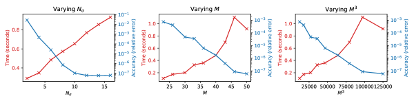
Our tunable parameters are then , , , and . We perform ablation experiments, modifying , , and individually with all the remaining parameters fixed. The results of these experiments are presented for and , respectively, in Figures 6.1 and 6.2. We take throughout; reference values for the other fixed parameters can be found in the captions.
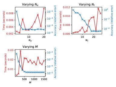

As expected, the time taken grows linearly in , , and , while errors decrease exponentially with , , and . As we increase one parameter individually, the error will eventually saturate. This is consistent with our understanding in Theorem 14, in which each of these parameters contributes roughly independently to the error in an additive fashion. In the one-dimensional case especially, there is some variance in the time taken; this is because the matvec is sufficiently fast that smaller effects such as constant setup times fail to fully amortize.
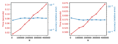
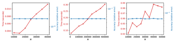
Finally, maintaining the parameters at their given reference values for each case , we vary . The results are presented in Figure 6.3, showing approximately linear scaling independent of dimension and a constant relative error. The reference values for , , and are the same as in Figures 6.1 and 6.2.
We comment that in higher dimensions, the memory bottleneck of our most basic implementation becomes nontrivial. This bottleneck owes to the formation of the tensor (cf. Remark 1). A sequential implementation, in which the sums over and are processed sequentially, could reduce the memory bottleneck to , but we do not pursue such modifications.
Since the relative error is empirically independent of , compatible with Theorem 14, we recommend an iterative approach to choosing parameters given a required error: repeatedly run test matvecs and increase one parameter, switching to another upon stagnation. This procedure can be employed for small and then the choices can be extrapolated to larger regression problems.
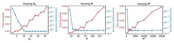
Next we consider the same experiments in the case of the squared-exponential kernel, for which it is unnecessary to choose and , and there is no need to vary . In this setting, , , and is determined accordingly. The results of the same ablation experiments for and are presented in Figures 6.4, 6.5, and 6.6 for dimensions , , and , respectively. Once again, we take throughout.
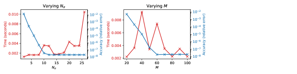
The time scaling in Figure 6.4 is not obvious because the error already saturates when and are both very small. Increasing the parameters to a size where the scaling is more readily apparent would not be useful.
Once again, as expected, the error decays exponentially in and , and the time grows linearly in and . Since the integration in no longer contributes to the error and since is larger (due to the fact that simply ), in this setting the error is smaller and the convergence with respect to is faster, and we quickly hit the lower bound determined by the tolerance .
Finally, again keeping all parameters at their given reference values (defined in Figures 6.4, 6.5, and 6.6) and varying , Figure 6.7 shows approximately linear scaling and constant relative error as in the Matérn case. For these experiments, we maintain relative accuracy of roughly independent of .
6.2 Solves
For the purposes of GPR, we are specifically interested in wrapping our kernel matvec subroutine in CG to compute the linear solve , cf. 1.1. Since the solve cost is fairly insensitive to the specification of , we simply draw the entries of independently from the uniform distribution on .
We compare our results for this inversion to those of the MATLAB package FLAM [17], which was the fastest out of all alternative strategies tested in [15]. In this section, we focus on the squared-exponential kernel. We set , since for the scaling of FLAM is linear in and we believe that it remains a state-of-the-art approach.
FLAM and our method take different approaches. FLAM first computes a block factorization of the entire matrix using elementwise queries. This is expensive but allows for fast matvecs and solves downstream. The Fourier method has insignificant offline cost but more expensive matvecs, and the solves require an iterative method wrapping the matvec subroutine. In order to compare the two, we consider the sum of both the on- and offline costs, i.e., the time necessary to go from no representation of at all to a complete solve .
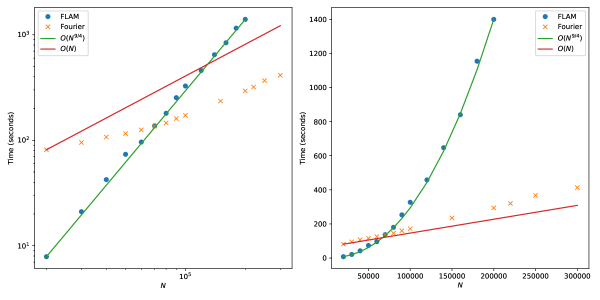
We consider two regimes, in both of which the condition number of the kernel matrix should remain approximately constant as grows. In the first, we take , specifically, , while maintaining a constant kernel. In this scaling regime, although we take an increasing number of observations, the noise of the observations also grows, such that our uncertainty about the inferred function remains constant. We fix , , and , and we choose a residual tolerance of in CG. These choices yield relative matvec errors that are never larger than .
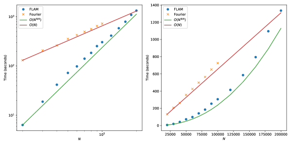
In the second scaling regime, we keep constant, but change the kernel as increases so that the effective number of nonzero entries in each row of remains constant and the diagonal entries of remain . Specifically, in terms of our reference choice for , we set and to fix the kernel. We set , independent of , and in order to maintain constant relative accuracy as is increased. These choices yield relative matvec errors that are never larger than . Again we choose a residual tolerance of in CG. FLAM allows us only one tunable relative error parameter, which we set to .
We report the comparison of the two approaches in Figures 6.8 and 6.9, which concern the first and second scaling regimes, respectively. These figures confirm the scaling of our method for our approach, while the scaling of FLAM is empirically about in both cases.
References
- [1] Sivaram Ambikasaran, Daniel Foreman-Mackey, Leslie Greengard, David W. Hogg, and Michael O’Neil. Fast Direct Methods for Gaussian Processes. IEEE Transactions on Pattern Analysis and Machine Intelligence, 38(2):252–265, February 2016.
- [2] Alex Barnett, Philip Greengard, and Manas Rachh. Uniform approximation of common Gaussian process kernels using equispaced Fourier grids. Applied and Computational Harmonic Analysis, 71:101640, July 2024.
- [3] Alex H. Barnett. Aliasing error of the kernel in the nonuniform fast Fourier transform. Applied and Computational Harmonic Analysis, 51:1–16, March 2021.
- [4] Alexander H. Barnett, Jeremy Magland, and Ludvig Af Klinteberg. A Parallel Nonuniform Fast Fourier Transform Library Based on an “Exponential of Semicircle” Kernel. SIAM Journal on Scientific Computing, 41(5):C479–C504, January 2019.
- [5] Albert P. Bartók, Mike C. Payne, Risi Kondor, and Gábor Csányi. Gaussian Approximation Potentials: The Accuracy of Quantum Mechanics, without the Electrons. Physical Review Letters, 104(13):136403, April 2010.
- [6] Gregory Beylkin and Lucas Monzón. On approximation of functions by exponential sums. Applied and Computational Harmonic Analysis, 19(1):17–48, July 2005.
- [7] John P Boyd. A fast algorithm for chebyshev, fourier, and sinc interpolation onto an irregular grid. Journal of Computational Physics, 103(2):243–257, 1992.
- [8] John P. Boyd. Chebyshev and Fourier spectral methods. Dover Publications, Mineola, N.Y, 2nd ed., rev edition, 2001.
- [9] Seok-Ho Chang, Pamela C. Cosman, and Laurence B. Milstein. Chernoff-Type Bounds for the Gaussian Error Function. IEEE Transactions on Communications, 59(11):2939–2944, November 2011.
- [10] Noel Cressie. Mission COntrol: A Statistical Scientist’s Role in Remote Sensing of Atmospheric Carbon Dioxide. Journal of the American Statistical Association, 113(521):152–168, January 2018.
- [11] A. Dutt and V. Rokhlin. Fast fourier transforms for nonequispaced data. SIAM Journal on Scientific Computing, 14(6):1368–1393, 1993.
- [12] Daniel Foreman-Mackey, Eric Agol, Sivaram Ambikasaran, and Ruth Angus. Fast and Scalable Gaussian Process Modeling with Applications to Astronomical Time Series. The Astronomical Journal, 154(6):220, December 2017.
- [13] Reinhard Furrer, Marc G Genton, and Douglas Nychka. Covariance Tapering for Interpolation of Large Spatial Datasets. Journal of Computational and Graphical Statistics, 15(3):502–523, September 2006.
- [14] Andrew Gelman, John B. Carlin, Hal Steven Stern, David B. Dunson, Aki Vehtari, and Donald B. Rubin. Bayesian data analysis. Chapman & Hall/CRC texts in statistical science. CRC Press, Boca Raton, third edition. edition, 2014. OCLC: 909477393.
- [15] Philip Greengard, Manas Rachh, and Alex Barnett. Equispaced Fourier representations for efficient Gaussian process regression from a billion data points, May 2023. arXiv:2210.10210 [cs, math, stat].
- [16] Matthew J. Heaton, Abhirup Datta, Andrew O. Finley, Reinhard Furrer, Joseph Guinness, Rajarshi Guhaniyogi, Florian Gerber, Robert B. Gramacy, Dorit Hammerling, Matthias Katzfuss, Finn Lindgren, Douglas W. Nychka, Furong Sun, and Andrew Zammit-Mangion. A Case Study Competition Among Methods for Analyzing Large Spatial Data. Journal of Agricultural, Biological and Environmental Statistics, 24(3):398–425, September 2019.
- [17] Kenneth Ho. FLAM: Fast Linear Algebra in MATLAB - Algorithms for Hierarchical Matrices. Journal of Open Source Software, 5(51):1906, July 2020.
- [18] Michael Kielstra and Michael Lindsey. Code for Gaussian process regression for common non-stationary kernels with log-linear scaling. https://doi.org/10.5281/zenodo.12638457, July 2024.
- [19] Per-Gunnar Martinsson. Fast Direct Solvers for Elliptic PDEs. Society for Industrial and Applied Mathematics, Philadelphia, PA, January 2019.
- [20] Victor Minden, Anil Damle, Kenneth L. Ho, and Lexing Ying. Fast Spatial Gaussian Process Maximum Likelihood Estimation via Skeletonization Factorizations. Multiscale Modeling & Simulation, 15(4):1584–1611, January 2017.
- [21] Marcus M. Noack, Harinarayan Krishnan, Mark D. Risser, and Kristofer G. Reyes. Exact Gaussian processes for massive datasets via non-stationary sparsity-discovering kernels. Scientific Reports, 13(1):3155, 2023.
- [22] Marcus M. Noack, Hengrui Luo, and Mark D. Risser. A unifying perspective on non-stationary kernels for deeper Gaussian processes. APL Machine Learning, 2(1):010902, 02 2024.
- [23] Marcus M. Noack and James A. Sethian. Advanced stationary and nonstationary kernel designs for domain-aware Gaussian processes. Communications in Applied Mathematics and Computational Science, 17(1):131–156, October 2022.
- [24] E. J. Nyström. Über Die Praktische Auflösung von Integralgleichungen mit Anwendungen auf Randwertaufgaben. Acta Mathematica, 54(0):185–204, 1930.
- [25] C Paciorek. Nonstationary Gaussian Processes for Regression and Spatial Modelling. PhD thesis, Carnegie Mellon University, Pittsburgh, PA, 2003.
- [26] Paciorek C and Schervish M. Nonstationary covariance functions for Gaussian process regression. In Thrun S, Saul L, and Schölkopf B, editors, Advances in Neural Information Processing Systems 16, pages 273–280. MIT Press, Cambridge, MA, 2004.
- [27] Carl Edward Rasmussen and Christopher K. I. Williams. Gaussian processes for machine learning. Adaptive computation and machine learning. MIT Press, Cambridge, Mass, 2006. OCLC: ocm61285753.
- [28] I. J. Schoenberg. Metric Spaces and Completely Monotone Functions. Annals of Mathematics, 39(4):811–841, 1938.
- [29] I. J. Schoenberg. Metric spaces and positive definite functions. Transactions of the American Mathematical Society, 44(3):522–536, 1938.
- [30] Y. Shih, G. Wright, J. Anden, J. Blaschke, and A. H. Barnett. cuFINUFFT: a load-balanced GPU library for general-purpose nonuniform FFTs. In 2021 IEEE International Parallel and Distributed Processing Symposium Workshops (IPDPSW), pages 688–697, Los Alamitos, CA, USA, jun 2021. IEEE Computer Society.
- [31] Michael L. Stein. Interpolation of Spatial Data. Springer Series in Statistics. Springer New York, New York, NY, 1999.
- [32] Lloyd N. Trefethen. Approximation theory and approximation practice. SIAM, Society for Industrial and Applied Mathematics, Philadelphia, extended edition edition, 2020.
- [33] Lloyd N. Trefethen and David Bau. Numerical linear algebra. Society for Industrial and Applied Mathematics, Philadelphia, 1997.
- [34] Lloyd N. Trefethen and J. A. C. Weideman. The Exponentially Convergent Trapezoidal Rule. SIAM Review, 56(3):385–458, 2014.
- [35] Ke Alexander Wang, Geoff Pleiss, Jacob R. Gardner, Stephen Tyree, Kilian Q. Weinberger, and Andrew Gordon Wilson. Exact gaussian processes on a million data points. Curran Associates Inc., Red Hook, NY, USA, 2019.
Appendices
Appendix A Glossary of notation
The following is a glossary of commonly used notation in our analysis. We think of , , , and as given. We think of , as well as and as tunable parameters controlling the error of the approximation. The other quantities are all induced in terms of these.
| Terms | Meaning |
|---|---|
| Spatial dimension | |
| Matérn parameter (2.4) | |
| , , | Parameters for discretization scheme (3.10) of integral |
| presentation (cf. (3.3) and (3.8)) of the Matérn kernel | |
| , , , | Parameters for Chebyshev interpolation by value of |
| , cf. (3.13); . | |
| Lebesgue constant for the Chebyshev interpolation scheme, cf. Definition 9 | |
| , | and , where is defined in (3.8) |
| , , | , , and |
| , | Parameters defining Fourier grid , cf. Section 3.3 |
Appendix B Integral presentation of the kernel
Here we verify (3.4). Recalling the definition of , we compute:
We can substitute the exact integration
to obtain
| (B.1) |
Appendix C Schoenberg presentation of the Matérn function
We want to show how to present such in the form of (3.3) for suitably chosen and .
It is useful to recall [31] that the Matérn function (2.4) can be more conveniently characterized in terms of a Fourier transform. Specifically, one can compute that
| (C.3) |
In the step indicated by we have used the identity for the inverse Fourier transform of a Gaussian.
Appendix D Background on NUFFTs
In our algorithms we will make use of non-uniform fast Fourier transforms (NUFFTs) [7, 11] of both type 1 and type 2, which are in fact formal adjoints of one another.
For our purposes, the type 1 NUFFT takes as input a vector of values associated to a scattered set of points and returns the object defined on elements of a truncated integer lattice by the formula By rescaling the scattered points , we can define the rescaled type-1 NUFFT:
which can be viewed as the evaluation of the unitary Fourier transform of the empirical distribution on the Fourier grid :
The type 2 NUFFT (including our rescaling convention), takes such a grid function as input and returns a vector of values associated to the scattered points, defined by:
Importantly, although the NUFFTs of type 1 and 2 are formal adjoints of one another, they are not inverses of one another.
Both types of NUFFT can be computed approximately (with prescribed accuracy) using standard libraries with computational cost [4]. All of our computations make use of the FiNUFFT library [4, 30, 3]. In this work, we assume for simplicity that we can compute NUFFTs exactly, neglecting this source of approximation error. We comment here that the scaling of the runtime of the NUFFT with respect to the prescribed error is merely logarithmic and can be easily accounted for. We elide this source of error simply for clarity of presentation.
Appendix E Proofs of technical lemmata
Proof of Lemma 3.
Without loss of generality assume that . Then letting with , we want to show that . Let be the -th row of , and let be such that . Then follows from for all . Finally, we can use Hölder’s inequality to bound
which completes the proof. ∎
Proof of Lemma 4.
Recalling our expression (3.7) for , our assumption (5.1) bounding , and our Matérn function presentation (3.8), compute:
In summary, by Definition 2 of the norm ,
| (E.1) |
Now, extending our definition to all integers (where we recall that ), we bound by the triangle inequality:
| (E.2) |
where in the last step we have used (E.1). In the last expression, the first error term measures the error of the infinite Riemann sum approximation of , while the last term measures the effect of cutting off the tails of the Riemann sum.
The impact of the tails can be bounded as follows. First compute:
so it follows that
| (E.3) |
as long as .
Next, note that by convexity, for any . Choose for arbitrary , yielding
Therefore
and it follows that
| (E.4) |
Then combining (E.3) and (E.4) with (E.2), we have that for any ,
| (E.5) |
It remains to bound the first term on the right-hand side of (E.5), i.e., the error of the infinite Riemann sum.
Specifically, we want to show that for any ,
| (E.6) |
which, together with (E.5), will complete the proof.
For simplicity, fix and define
| (E.7) |
Then, by our expression (3.7) for , our assumption (5.1) bounding , and our Matérn function presentation (3.8), it suffices to show that the error of the infinite Riemann sum for is , independent of .
Standard results [34] guarantee that if we extend analytically to a strip
where and can find bounding
uniformly over , then the error of the Riemann sum is bounded by
We will take , so the proof is complete once we can show that
| (E.8) |
independent of and .
For with , let us us bound the size of the first factor in the definition (E.7) of , using the fact that :
| (E.9) |
Now
and since , we have , and therefore . Moreover, the power is non-negative, so the entirety of (E.9) is bounded by on , i.e.,
| (E.10) |
for where .
Next, let us us bound the size of the second factor in the definition (E.7) of :
Now , so , so
| (E.11) |
The right-hand side is integrable since and independent of , as well as the choice of , so we have achieved (E.8) and the proof is complete. ∎
Proof of Lemma 6.
Our proof will leverage the well-known error bound for Chebyshev interpolation given by Theorem 8.2 of [32]. To use this error bound, we make a few preliminary comments. First, recall that the Bernstein ellipse of radius is defined to be the subset
of the complex plane.
Second, let be the affine transformation that maps the standard reference interval for Chebyshev interpolation to our interpolation interval . We can view this map as extending to the entire complex plane. We allow ourselves to abuse notation slightly by considering both as a map and a variable, and the suitable interpretation should be clear from context.
Now Theorem 8.2 of [32] directly implies that if there exists some constant such that for all and all , then
| (E.12) |
for all and all . Therefore, we want to find constants and such that the bound
| (E.13) |
holds for all and .
To achieve this, we start by writing for . Then
where we have defined . Further define and , so that
Then we can write
It will follow that
as long as we can guarantee that .
Then we claim that under the choice
| (E.14) |
the desired inequality (E.13) holds with . The preceding argument establishes that to prove this claim, it suffices to show that whenever .
To wit, we want to show that
for all . To see this, in turn it suffices to show that
Now recall that any satisfies and . Thus in turn it suffices to show that
| (E.15) |
Algebraic manipulations verify that the choice (E.14) ensures that (E.15) holds with equality.
Therefore (E.13) holds with and . Since in turn , the statement of the lemma directly follows from substitution and simplification. ∎
Proof of Lemma 10.
Proof of Lemma 11.
For all , define
so that (defined as in (3.15)) satisfies
Moreover, let denote the Fourier transform of this function.
Define the index set for our Fourier grid, and let denote the Fourier grid points themselves for .
Then observe that
and meanwhile
Therefore to prove the lemma, we simply need to bound the error of the trapezoidal rule on our Fourier grid defined by for the integration of the function
independently of , , and . We will write for notational simplicity. Concretely then we want to bound the integral error
We can compute directly the Fourier transform of the Gaussian
and hence also the analytical formula
| (E.17) |
Then bound
| (E.18) |
The first term on the right-hand side of (E.18) measures the error of the infinite Riemann sum approximation of . The second term measures the effect of cutting off the tails of .
To bound the second term, we deduce from (E.17) that
| (E.19) |
from which it follows111We can bound using (E.19), for a suitable constant . Then we can bound the sum over with the sum of the sums over each of the ‘slab complements’ for , which are all equal, yielding: assuming and using the fact [9] that . that the tail term can be bounded as
| (E.20) |
assuming that .
Now to bound the first term on the right-hand side of (E.18), we use the Poisson summation formula, which implies that
| (E.21) |
where is the inverse Fourier transform of , which can be calculated explicitly as
| (E.22) |
Note moreover that , so from (E.21) it follows that
| (E.23) |
Now from the expression (E.22) for we deduce that
| (E.24) |
using the fact222This fact in turn follows from the identity , which holds when , together with similar reasoning in the opposite case. that .
Then recall that we assume , so in turn it must be the case that . Therefore from (E.24) and the reverse triangle inequality we have that
| (E.25) |
from which it follows333From (E.23) and (E.25) we can bound , for a suitable constant . Then again we can bound the sum over with the sum of the sums over each of the ‘slab complements’ for , which are all equal, yielding: Now if , then again using the fact that . Then since we treat as constant. that can be bounded as
provided that . Combining with (E.20) in (E.18) completes the proof. ∎
Proof of Lemma 13.
We employ definition 3.18 to write
We want to continue our calculations to derive a suitable bound on .
Appendix F Proof of Theorem 14
Proof of Theorem 14.
We will focus first on the general Matérn case.
By the triangle inequality, we bound
The bound is justified because the underbraced expression is precisely , following (3.19). Let the three terms on the right-hand side be denoted , , and , respectively.
First we cite Lemma 4, which establishes that
| (F.1) |
Finally, using Lemma 13, we bound:
Again using the fact that , we conclude that
| (F.3) |
Combining (F.1), (F.2), and (F.3), we conclude that
as was to be shown.
The logic in the case of the squared-exponential kernel is exactly the same, except that there is no integration over and so the first error term () is discarded. ∎