Three-dimensional Imaging of Pion using Lattice QCD: Generalized Parton Distributions
Abstract
In this work, we report a lattice calculation of -dependent valence pion generalized parton distributions (GPDs) at zero skewness with multiple values of the momentum transfer . The calculations are based on an gauge ensemble of highly improved staggered quarks with Wilson-Clover valence fermion. The lattice spacing is 0.04 fm, and the pion valence mass is tuned to be 300 MeV. We determine the Lorentz-invariant amplitudes of the quasi-GPD matrix elements for both symmetric and asymmetric momenta transfers with similar values and show the equivalence of both frames. Then, focusing on the asymmetric frame, we utilize a hybrid scheme to renormalize the quasi-GPD matrix elements obtained from the lattice calculations. After the Fourier transforms, the quasi-GPDs are then matched to the light-cone GPDs within the framework of large momentum effective theory with improved matching, including the next-to-next-to-leading order perturbative corrections, and leading renormalon and renormalization group resummations. We also present the 3-dimensional image of the pion in impact-parameter space through the Fourier transform of the momentum transfer .
I Introduction
Since its discovery in 1947, the pion has been the subject of intense research, recognized for its dual identity as both a Goldstone boson linked to chiral symmetry breaking and a QCD-bound state. Over the years, substantial efforts have been dedicated to studying its internal structure by analyzing experimental data. Key methodologies have involved extracting form factors (FFs) through the pion-electron scattering [1] and discerning parton distribution functions (PDFs) via the Drell-Yan process [2]. However, these approaches are limited to revealing only the one-dimensional structure of the hadron. For a more comprehensive, three-dimensional perspective, the focus has shifted to generalized parton distributions (GPDs), a concept introduced in the 1990s [3, 4, 5, 6]. Access to GPDs is typically gained through exclusive reactions, notably deeply virtual Compton scattering [6] and deeply virtual meson production [7, 8].
Presently, a series of experiments are being conducted or planned, which can enrich our understanding of the pion internal structure. Prominent among these are the JLab 12 GeV program [9], the Apparatus for Meson and Baryon Experimental Research (AMBER) at CERN SPS [10], the forthcoming Electron-Ion Collider (EIC) at Brookhaven National Laboratory [11], and the Electron-Ion Collider in China (EicC) [12]. These initiatives are designed to probe the pion structure in various kinematic regimes. However, extracting GPDs from experimental data is fraught with challenges, including the chiral-odd nature of certain distributions, such as the transversity GPDs, and the complexity involved in pion production. On the other hand, lattice QCD results, offering complementary insights and potentially guiding experimental efforts, are highly sought after. The advent of Large Momentum Effective Theory (LaMET) [13, 14, 15] in 2013 made it possible to directly calculate the Bjorken- dependence of the parton distributions, extending the scope of GPD studies beyond just the first few Mellin moments [16, 17, 18, 19, 20, 21, 22, 23, 24, 25]. This spurred a flurry of lattice research on nucleon and meson GPDs [26, 27, 28, 29, 30, 31, 32, 33, 34] based on the quasi-distribution (see reviews in Refs. [15, 35]), which is defined in terms of matrix elements of non-local operators involving quark and antiquark fields separated by a spatial distance, rather than a light-cone distance, and thus is calculable on the lattice.
While there are several lattice QCD studies of the nucleon GPDs [27, 28, 29, 30, 31, 33, 34], including a few based on alternate methods [36, 37, 38, 39], there have been limited LaMET calculations of the pion GPDs [26, 32]. Traditionally, GPD calculations are conducted in the Breit (symmetric) frame, requiring the momentum transfer to be symmetrically distributed between the initial and final states. However, this approach incurs substantial computational costs. Recently, a frame-independent method was proposed to extract GPDs from lattice calculations in an arbitrary frame [30]. This innovative approach holds the potential to significantly reduce computational expenses by working in a non-Breit (asymmetric) frame where the initial or final state momentum is fixed.
Two crucial aspects of obtaining the light-cone parton distributions from the lattice calculations are the renormalization and matching process. The GPDs and quasi-GPDs (qGPDs) are typically defined in different renormalization schemes. For the qGPDs extracted from the lattice analyses, renormalization is required to eliminate the ultraviolet (UV) divergences stemming from the Wilson line. Commonly employed renormalization methods include the regularization-independent momentum-subtraction (RI/MOM) [40, 41, 42, 43] and various ratio schemes [44, 45, 46, 47, 48]. However, these methods adhere to a factorization relation with the light-cone correlation only at short distances. At long distances, they introduce nonperturbative effects [49], which will impact the qGPDs through the Fourier transform of the matrix elements, thereby affecting the LaMET matching results in Bjorken- space. To overcome this issue, in this work, we use a hybrid-scheme renormalization [49]. The key point of this scheme is to renormalize the matrix elements at short and long distances separately, which can remove the linear divergence at long distances without introducing additional nonperturbative effects.
Furthermore, we match the qGPDs in the lattice renormalization scheme to the light-cone GPDs in the scheme through LaMET [50, 51, 52, 53]. During this process, the accuracy of the perturbative calculation plays a significant role in the precision of the final GPD results. In the zero-skewness limit, the matching kernel of GPDs is the same as the one for PDFs [51], which has been derived up to the next-to-next-to-leading order (NNLO) [47, 54]. We also utilize renormalization group resummation (RGR) [55, 56] to resum the small- logarithmic terms. Additionally, we consider leading-renormalon resummation (LRR) [57, 58], which can remove the renormalon ambiguity in the Wilson-line mass matching, to eliminate the linear power corrections [58]. Therefore, we achieve a state-of-the-art calculation of the valence pion GPDs using an adapted hybrid-scheme renormalization, along with the implementation of the combined NNLO+RGR+LRR matching.
In this study, we present our lattice calculations of the valence pion GPDs using the LaMET approach, featuring a very small lattice spacing of 0.04 fm within the non-Breit frame. The organization of this paper is as follows: In Section II, we review the definitions of pion GPDs and qGPDs in an arbitrary frame, outline our lattice setup, and describe the methodologies employed to extract the matrix elements from the combined analyses of the two-point and three-point correlation functions. In this section, we also detail the renormalization procedure of the qGPD matrix elements in the coordinate space using the hybrid scheme and discuss the challenges of performing the Fourier transform to get the qGPDs. Subsequently, we apply the LaMET matching approach to derive the valence light-cone GPDs in Section III. This section contains our main results, including the sensitivity of our results to the perturbative accuracy of the matching and the dependence on the renormalization scales. Finally, Section IV provides a summary of our findings.
II Valence pion quasi-GPDs in asymmetric frame on the lattice
II.1 General considerations
Our goal is to calculate the valence pion GPDs in an asymmetric frame using the frame-independent approach laid out in Ref. [30]. For this, we consider the following non-local iso-vector matrix element
| (1) |
where represents the Lorentz indices, and are the initial and final momenta of the pion, respectively, , , and
| (2) |
where is the Wilson line that connects the quark and antiquark fields, ensuring the gauge invariant of the matrix element. Here, we use the following normalization of the pion states . Following Ref. [30], we write the matrix element in terms of the Lorentz-invariant amplitudes for , as follows:
| (3) |
The coordinate space light-cone valence pion GPDs is usually defined in terms of as , i.e. the momentum space light-cone GPDs is written as
| (4) |
where the skewness parameter and . However, it is possible to define the light-cone GPDs in a frame-independent, i.e., Lorentz-invariant way [30] as
| (5) |
Motivated by this, the Lorentz-invariant definition of qGPDs can be written as
| (6) |
This is a natural choice for the qGPDs because in the light-cone limit , it should be equal to the light-cone GPDs up to the leading order in
| (7) |
In the Lorentz-invariant framework, the momentum-space GPD is defined as [30]
| (8) |
and similarly for qGPD
| (9) |
By studying the behavior under hermiticity and time-reversal transformations simultaneously, it was found that the amplitude is an odd function of [30, 33]. In the forward limit, GPDs should smoothly approach PDFs, implying that should be equal to 0 in this work at zero skewness. In the following subsections, we will discuss our lattice setup and lattice QCD results on .
II.2 Lattice setup
Our lattice calculations use the gauge ensembles provided by the HotQCD collaboration [59], utilizing a 2+1 flavor setup with Highly Improved Staggered Quark (HISQ) action [60]. The lattice configuration has dimensions of and a lattice spacing of fm. The sea quark masses are adjusted to yield a pion mass of 160 MeV. In the valence sector, we use the Wilson-Clover action with one level of hypercubic (HYP) smearing [61]. For the coefficient of the clover term, we utilize the tree-level tadpole-improved value computed with the fourth root of the plaquette, yielding 1.02868 [62]. The valence quark masses in the Wilson-Clover action are tuned to , resulting in a pion mass of 300 MeV.
Central to our computational approach is the use of momentum-boosted smeared sources [63]. The quark propagators are obtained through the application of the multigrid algorithm [64] to invert the Wilson-Dirac operator using the QUDA software suite [65, 66, 67] on GPUs. In this work, we consider the pion boosted along the -direction with momenta with being an integer. To obtain a good signal for the boosted pions, momentum-boosted sources and sinks are constructed using a Gaussian profile, with boost momenta in the -direction. Source construction is done in the Coulomb gauge, and the Gaussian profile is created with the radius of 0.208 fm [68, 62]. Employing these quark propagators, we have computed both the two-point and three-point hadron correlation functions. To increase statistics per configuration, we combined multiple exact (high-precision) and sloppy (low-precision) samples and implemented the all-mode averaging (AMA) technique [69]. The lattice parameters used in this study are summarized in Table 1.
We can get the matrix elements by analyzing the two-point and three-point correlation functions. The two-point correlation function is defined as
| (10) |
where denotes the spatial momentum, and represent the spatial coordinates, and and correspond to the time coordinates. Here, and stand for the pion creation and annihilation operators, respectively, with the subscript “” indicating “smeared”. The three-point correlation function is defined as
| (11) |
where and denote the spatial final momentum and momentum transfer, respectively. The spatial initial momentum is given by . The quark bilinear operator, , defined in Eq. (2), is also characterized by its spacetime insertion position (). In this work, we only consider the case of zero skewness, that is, and . For each value of , we consider several values of . The different choices of momenta used in our study are summarized in Table 1, including the momentum transfer in physical units. As one can see from the table, for the smallest non-zero value of , we have performed calculations in both Breit and non-Breit frames at very similar values of .
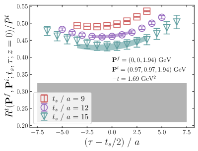
The approach used to obtain the pion matrix element here closely follows our previous works [62, 70, 71, 72, 73, 74]. We fit the large behavior of the two-point correlation functions with two or three states and obtain the energies of these states for different momenta. The corresponding energy levels are then used in the analysis of the three-point function and the extraction of the pion matrix elements . We consider the following ratio of
| (12) |
where and correspond to the ground-state pion energies in the initial and final states, respectively, and the kinematic factor is used for the normalization. For large and , this ratio gives the matrix element . We assume that for large and , two or three states mainly contribute to and perform the corresponding fits to obtain the matrix element. Some details of the fits are provided in Appendix A.
| Frame | [GeV] | [GeV2] | #cfgs | (#ex, #sl) | ||||
| Breit | 9,12,15,18 | (1, 0, 2) | 2 | 0.968 | (2, 0, 0) | 0.938 | 115 | (1, 32) |
| non-Breit | 9,12,15,18 | (0,0,0) | 0 | 0 | (0,0,0) | 0 | 314 | (3, 96) |
| 9,12,15,18 | (0,0,2) | 2 | 0.968 | (1,2,0) | 0.952 | 314 | (4, 128) | |
| 9,12,15 | (0,0,3) | 2 | 1.453 | [(0,0,0), (1,0,0) (1,1,0), (2,0,0) (2,1,0), (2,2,0)] | [0, 0.229, 0.446, 0.855, 1.048, 1.589] | 314 | (4, 128) | |
|---|---|---|---|---|---|---|---|---|
| 9,12,15 | (0,0,4) | 3 | 1.937 | [0, 0.231, 0.455, 0.887, 1.095, 1.690] | 564 | (4, 128) |
II.3 Lattice results on the Lorentz-invariant amplitudes
Having determined the matrix elements for different values of the kinematic variables in Eq. (3), we can deduce the Lorentz-invariant amplitudes . The results of obtained from the Breit and non-Breit frames with comparable values of should be consistent. Therefore, we select two sets of lattice data from different frames, as shown in the first and third rows of Table 1, which have identical values of and very close values. The dataset from the Breit frame has GeV2, while the dataset from the non-Breit frame has GeV2. According to Eq. (3) and in our case, for the non-Breit frame, we can simultaneously solve and by combining the data of and components. For the Breit frame with and , we can directly get and from and components, respectively.
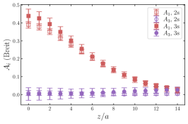
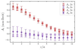
The amplitudes obtained from these two datasets with GeV are shown in Fig. 1. The left two panels show the results obtained using both 2-state and 3-state fits within the Breit and non-Breit frames, respectively. The 2-state fit results are represented by the open symbols, while the 3-state fit results are denoted as the filled symbols, labeled as “2s” and “3s” in the figure, respectively. One can see that the contamination from the excited states is apparent in the Breit frame, so the 3-state fit is needed. For the non-Breit frame, it can be seen that these two kinds of fit results are comparable within 1- error, and the 2-state fit results are more stable. In both frames, we find that is zero within error, as expected. In the right panel of Fig. 1, we investigate the frame independence of by selecting the 3-state fit results for the Breit frame and the 2-state fit results for the non-Breit frame. Furthermore, since we observe that is compatible with zero within errors also for the non-Breit frame, we perform the extraction of from the non-Breit frame based on setting and using the component. The results from this analysis are shown as the green triangles in the right panel of Fig. 1. As depicted in the figure, the non-Breit frame results, both with and without setting , exhibit good agreement and also are consistent with the Breit frame results.
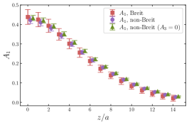
Therefore, we conclude that it is possible to obtain from the calculations in the non-Breit frame by initially setting to zero. Specifically, since in our lattice QCD calculations, both the initial and final pion states are boosted along the direction by an equal amount , the Lorentz-invariant definition for the coordinate-space qGPDs for can be directly expressed as
| (13) |
For convenience, we denote the dimensionless matrix element as hereafter.
Since we aim to get the valence pion GPDs within the LaMET framework, we selected the two largest available momenta in the non-Breit frame for our calculations, as detailed in the last two rows of Table 1. Additionally, these two datasets can be used to study the dependence of the final light-cone GPDs, which can reflect the effectiveness of our perturbative matching, as discussed later. For each momentum, we analyzed six values of the momentum transfer . Using the matrix elements we have obtained, several steps are required to derive the qGPDs, including renormalization, extrapolation for the large region of , and the Fourier transform. Subsequently, the light-cone GPDs can be obtained from the qGPDs using the LaMET.
II.4 Renormalization
As we mentioned before, the renormalization of the qGPD matrix elements is crucial for removing the UV divergences from the Wilson line as well as for matching to the light-cone GPDs, which are usually defined in the scheme. Since the non-local quark bilinear operator is multiplicatively renormalizable, if we call the matrix elements extracted directly from the lattice calculations as the bare matrix elements, the relation between the bare and renormalized matrix elements can be expressed as [75, 76, 77, 49]
| (14) |
where the superscripts “B” and “R” denote the “bare” and “renormalized” quantities, respectively, includes the -independent logarithmic divergence, the term with accounts for the linear divergence, and the term with is introduced to address the scheme dependence of and to match the lattice scheme to the scheme [78, 70, 57, 58]. Theoretically, should be a constant and independent of .
The hybrid scheme renormalization is defined by merging the ratio scheme for short distances with the explicit subtraction of self-energy divergences in the Wilson line for long distances [49]
| (15) |
Here, represents the position where the ratio scheme is matched onto the explicit subtraction of the divergence in the Wilson line, which is part of the renormalization scheme. To reduce artifacts and improve the signal, we can further divide by the renormalized electromagnetic form factor such as
| (16) |
Notably, we need to multiply back into our results when calculating the pion qGPDs, as presented in the next subsection.
At short distances, all the divergences can be directly canceled by such a ratio. However, for long distances, in order to perform the renormalization, we first need to determine the values of and . In line with our previous studies, we determine using lattice QCD results on the static quark-antiquark potential and the free energy of a static quark at non-zero temperatures [79]: for fm lattice [70]. The value of can be obtained using the bare matrix element results at zero momentum and zero momentum transfer. Namely, by comparing the lattice computations at with their corresponding Operator Product Expansion (OPE) expressions for such a ratio
| (17) |
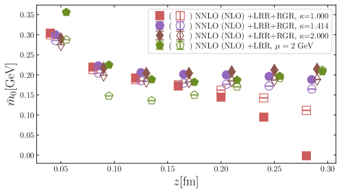
where is the anomalous dimension of the quark bilinear operator, known up to three loops [80], and the expressions for and can be found in Appendix B, we can extract the values of . Here, we set . The use of the zero momentum matrix element results in only the 0-th Wilson coefficient remaining, which is calculated up to the NNLO [47, 54]. Furthermore, we have incorporated RGR [55] at the next-to-next-to-leading-logarithm (NNLL) accuracy. The RGR allows us to effectively sum the large logarithmic terms arising in the perturbative expansions and to evolve the running coupling from the physical scale to the factorization scale = 2 GeV. Here, is a proportionality constant, and is the usual Euler constant. In principle, we should choose to match the natural physical scale , but we found that Eq. (17) with cannot describe the lattice data with a constant in . Therefore, to estimate the scale variation uncertainty, we choose our central value of as 1.414 and vary it between 1 and 2, where the strong coupling constant remains reasonably small ( 0.3) at the short distances we considered. Additionally, we include LRR [58, 57] in the Wilson coefficient that captures the dominant contributions from renormalons and improves the convergence properties of the perturbative series [58].
In Fig. 2, we show the results of obtained with NNLO(NLO)+LRR and NNLO(NLO)+LRR+RGR Wilson coefficients. As mentioned before, is excepted to be a constant and independent of . However, in practice, this is not always the case for all values, as illustrated in Fig. 2. For the two smallest values of , we observe lattice artifacts in the determination of , as expected. However, the dependence of on becomes much milder for larger values. The only exception is the case , where the running coupling becomes very large for 0.2 fm, causing the perturbative expansions for the Wilson coefficients to break down. The values of determined using NLO+LRR also show some dependence on due to missing higher-order corrections. However, thanks to LRR, the dependence of on is significantly reduced already at this level compared to our prior analyses of the pion PDFs [70]. All other determinations of obtained with are consistent with each other and show very small -dependence for fm. In the following, we will take the results at fm to perform the hybrid-scheme renormalization. For example, is taken in the case of NNLO+LRR+RGR (). We also choose fm as our default choice for the hybrid scheme.
II.5 Large extrapolation and Fourier transform
In this work, our aim is to get the valence light-cone GPDs in momentum () space. In the isospin symmetric limit, the valence light-cone GPDs, as well as qGPDs, are equal to the isovector GPDs, as discussed in Ref. [68]. To obtain the momentum-space isovector (valence) qGPDs, we need to perform a Fourier transform on of the coordinate-space isovector qGPDs
| (18) |
where is the valence pion qGPDs, and the factor of 2 at the beginning of the middle formula comes from the definition of in Eq. (2) and the fact that the integral of the valence quark distribution in the momentum space from to should be one.
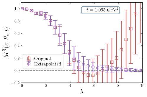
In Fig. 3, we present our results of the renormalized matrix elements, denoted by the red square symbols, as a function of . Due to the large statistical errors at large and the finite volume effects, we can reliably calculate the renormalized matrix elements only up to a certain value of . This prevents us from performing the Fourier transform directly on . To address this problem, we perform an extrapolation of the renormalized matrix elements from a truncation position and replace the lattice results with the extrapolated values for . We expect that should vanish exponentially at large [49, 70], which means that the extrapolation mainly affect the small- region of GPDs [70]. Therefore, we fit the lattice results of at large using the following ansatz
| (19) |
where are the fit parameters. In practice, we choose 6 data points above a critical position where the matrix element results become unreliable, such as showing negativity or lacking a decaying trend, to do the fit. Subsequently, employing this decay model with the fitted parameters, we simulate results starting from the truncation position , which is the midpoint of the fit range, and extend towards long distances where the matrix element approaches zero. We constrain the fit parameters with the priors and extrapolate the data to , which can lead to extrapolated results decaying to zero in most cases. However, in the cases of GeV2 for GeV, due to the slower decay, we need to impose a stricter constraint GeV [70] as a fit prior and extrapolate the matrix elements to a longer distance . The extrapolated results, indicated by the purple circle symbols in Fig. 3, exhibit desired decay behavior at long distances and start to approach zero as the distances become sufficiently large. Therefore, the extrapolation can correct the artificial behavior of the lattice data at large .
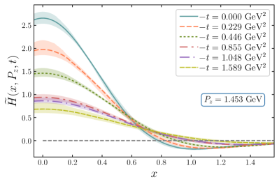
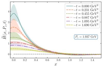
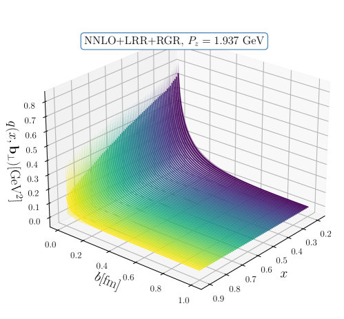
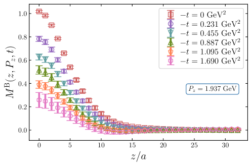
To obtain the dependence of the qGPDs, we need to integrate the extrapolated renormalized matrix elements over all values of in the Fourier transform. In Fig. 4, we show the valence pion qGPD results at and 1.937 GeV, which are obtained using NNLO+LRR+RGR () renormalization. We present results for six values corresponding to each value. We see that as increases, the distributions start at smaller values and decay slower with increasing . If we compare the data with similar sizes between these two panels, we can find that there are considerable differences between GeV and GeV results. We expect that the perturbative matching to light-cone GPDs, discussed in the next section, can correct for a significant portion of these differences.
III Numerical results on the valence pion light-cone GPDs
We utilize the LaMET approach for the perturbative matching of qGPDs to the light-cone GPDs
| (20) | ||||
where , and are the inverses of the DGLAP evolution kernel and the hybrid-scheme matching kernel, respectively. The detailed expressions for these kernels up to the NNLL accuracy are given in Appendix B.
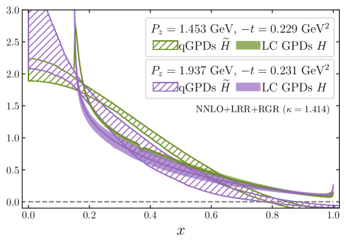
Since the qGPDs vanish at the positive and negative infinities, the integration range is finite in practice. To obtain numerical results on the light-cone GPDs, we can discretize the integration variables and replace the integrals with sums, as shown in the second line of Eq. (20). This procedure can reproduce the exact numerical integration well [70]. In Fig. 5, we demonstrate both qGPD and light-cone GPD results obtained from NNLO+LRR+RGR () perturbative matching with three-loop DGLAP evolution [81, 82]. It shows the results from two datasets with different values of but similar values of . As seen from this figure, there is a significant difference in the dependence between the qGPDs and light-cone GPDs, especially at lower . The effects of the matching are most significant at small and large values of . Additionally, the dependence of the distributions is significantly reduced after matching, as expected. The slight dip in the solid-filled green band is likely a numerical artifact, which should be smooth judging by the smoothness of results nearby. In this figure, we only show the results for the light-cone GPDs for for the reasons that will be explained below.
Since a larger is favored for better control of power accuracy, we will focus on the case with the largest momentum GeV in the following discussion. We will explore the dependence of the light-cone GPDs on the matching accuracy, renormalization scale, and physical variables.
III.1 The dependence of the light-cone GPDs on the perturbative accuracy of the matching and the renormalization scale
In this subsection, we examine the sensitivity of the pion light-cone GPDs to the perturbative accuracy in the matching and the renormalization scale, aiming to determine the reliability of our results.
In Fig. 6, we present the light-cone GPD results for the largest momentum GeV, obtained using NLO and NNLO perturbative matching with LRR, both with or without RGR. The line-filled bands represent the results obtained without RGR at GeV. The solid-filled bands show the results obtained with RGR, considering the variation of . The darker-solid-filled bands display the statistical errors with only, while the lighter-solid-filled bands also include additional systematic errors associated with scale variation from to 2. The scale variation of the results is more significant at small and large . We have selected the data with the smallest and largest momentum transfers for a clearer comparison. The NNLO results exhibit smaller scale variation, particularly for data with larger values. Moreover, the results with and without RGR are almost consistent in the intermediate region. However, they have a significant difference for . Since at low scales, the strong coupling constant and the logarithms diverge in the case of RGR, causing the perturbation theory to break down. Consequently, our light-cone GPD results obtained with RGR are only reliable for . The RGR also plays a role in the vicinity of . In this region, the threshold logs may also be important [55, 83]. However, threshold resummation is beyond the scope of this work. Finally, we note that the results between the NLO and NNLO display convergence, especially for the case with larger value.
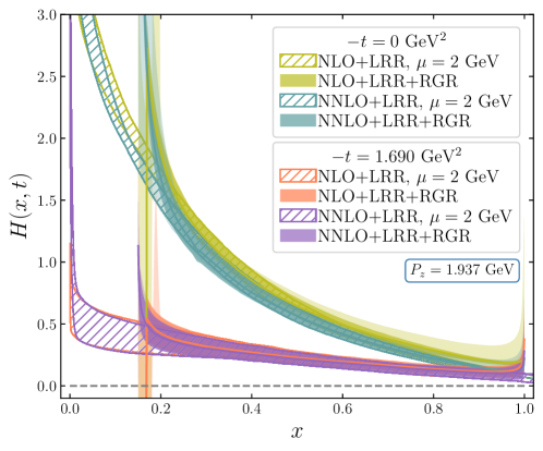
If one uses the hybrid scheme to perform the renormalization, the resulting light-cone GPDs may depend on the choice of . Therefore, it is important to check the dependence of our results on . We compare the valence light-cone GPD results with three different values of for GeV in Fig. 7. As a demonstration, we show our results for GeV2, obtained using NNLO+LRR+RGR. The lines represent the central values obtained with , while the bands encompass both statistical and systematic errors. This convention for the error bands is used in the subsequent figures as well. We can see that the final valence light-cone GPD results have little dependence on . The situations are similar for other values of . Thus, our findings are not sensitive to the choice of . Since the value of at shows the smallest dependence on the perturbative order and the renormalization scale, we adopt for the following analyses.
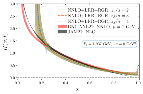
Furthermore, the zero momentum transfer case corresponds to the PDF results, allowing for comparison with previous PDF calculations. Specifically, we compare our findings with the global analysis at NLO accuracy (JAM21) [84] and our previous results using the NNLO matching (without LRR or RGR) within the same lattice framework (BNL-ANL21) [70]. Our results agree well with the global fit results for . Regarding the comparison with BNL-ANL21, differences for are not surprising, as discussed earlier. Additionally, we observe that the results obtained with LRR and RGR in this work show a slight downward shift compared to previous findings in the intermediate region, while they slightly exceed previous results for .
III.2 The -dependence of the light-cone GPDs
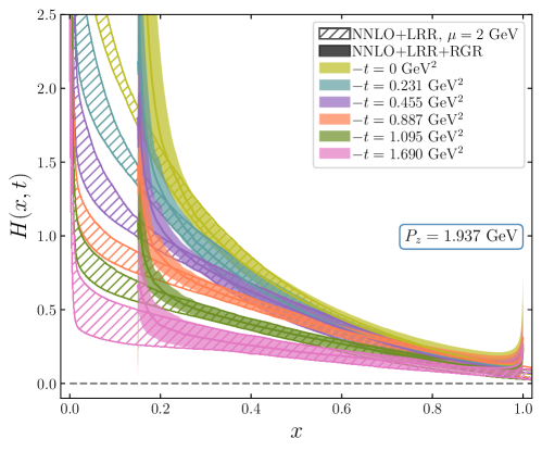
Having analyzed the systematic effects in the determination of the valence pion light-cone GPDs at some representative values of , we can now study the entire dependence of the light-cone GPDs in more detail. In Fig. 8, we present the valence light-cone GPDs as a function of the Bjorken- across all the available values of . As expected from the previous discussion, for , there are significant differences in all results between the cases with (solid-filled bands) and without (line-filled bands) RGR. The distributions exhibit significant dependence on and . Firstly, the light-cone GPDs decrease as increases for a fixed . Secondly, the fall-off of the GPDs along is notably reduced at larger values of . Similar behavior of the pion GPDs was also found in Ref. [32], where a lattice spacing of fm and a symmetric frame were utilized.
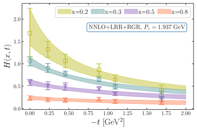

To further explore the and dependence of the pion valence light-cone GPDs, we would like to parametrize our results with a suitable ansatz. Based on past experience with the pion form factor [71], we employ the monopole form
| (21) |
where represents the GPDs at zero momentum transfer, equivalent to the PDFs, and is a -dependent monopole mass parameter, which is related to the pion effective radius as , in analogy to the usual pion charge radius. This fit ansatz works very well, as demonstrated by the bands in the left panel of Fig. 9. The left panel displays the dependence of the light-cone GPDs for four selected values of , namely , and 0.8. The lattice results are shown as the data points, and the corresponding monopole fit results are displayed as the bands. We can observe that the dependence of the valence light-cone GPDs becomes milder as increases. For , almost no dependence can be discerned within the estimated errors. The results of the pion effective radius are shown in the right panel of Fig. 9. The effective radius clearly decreases with increasing . This means that when quarks have higher momentum fractions, they are likely to be confined to a smaller spatial region in the transverse plane. This confinement results in narrower distributions in position space, potentially reducing the effective radius. Interestingly, the effective radius for is comparable to the pion charge radius obtained from the pion electromagnetic form factor, specifically fm2, as calculated in Ref. [71] using the same pion mass.
Moreover, the Fourier transform of the valence light-cone GPDs at zero skewness, with respect to the transverse components of the momentum transfer, defines the valence impact-parameter-space parton distributions (IPDs):
| (22) |
where is the impact parameter. The IPDs describe the probability density of finding a parton with momentum fraction at a specific transverse distance from the center of the transverse momentum (CoTM). They can offer a comprehensive view of the parton distributions in both momentum and coordinate spaces within the hadron. Using our monopole fit results of , we can perform a Fourier transform in to obtain the valence IPDs. Fig. 10 shows the results with varying from 0.2 to 0.9 and from 0 to 1 fm. We can find that when the partons carry a larger momentum fraction , the distributions are more localized, which results in a more concentrated distribution in the impact-parameter space. Conversely, as decreases, the distributions become broader in , indicating a more diffuse spatial distribution of lower-momentum quarks.
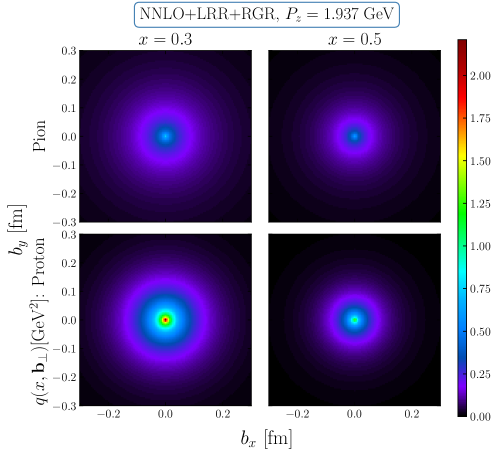
It is interesting to compare the pion valence IPDs with those of the proton, as shown in Fig. 11. We display the comparison in a two-dimensional distribution at and 0.5. The light-cone proton GPDs data are from Ref. [85]. We perform a dipole fit on the proton GPDs and then get the corresponding IPDs through the Fourier transform. For both the pion and proton, the distributions become more concentrated at larger , corresponding to smaller effective radii, which is consistent with our findings from the right panel of Fig. 9. Comparison of the proton and pion results at fixed reveals that the proton exhibits a broader distribution of valence quarks than the pion at both and 0.5. To some extent, this observation relates to the fact that the charge radius of the proton is larger than that of the pion. Fig. 11 also indicates that the valence quark distributions within the pion are somewhat less peaked at the very center compared to those within the proton.
IV Conclusions
We study the pion valence light-cone GPDs using the LaMET approach at a lattice spacing of 0.04 fm, which is more than two times smaller than the lattice spacing used in other studies of pion GPDs ( fm) [32]. In this work, we utilize the Lorentz-invariant definition of the GPDs, enabling us to perform calculations in the non-Breit frame. This approach enables simultaneous calculation of multiple momentum transfers and thus significantly reduces the computational costs. In this work, we perform calculations within both the Breit and non-Breit frames. By comparing the amplitude results of these two frames, we demonstrated once again the validity and efficacy of the Lorentz-invariant approach. To obtain the pion valence light-cone GPDs from the qGPDs, we use NNLO hybrid-scheme matching along with leading renormalon resummation and renormalization group resummation. The use of leading renormalon resummation significantly reduces the perturbative uncertainty in the hybrid renormalization scheme. Furthermore, the use of renormalization group resummation allows us to determine the range of Bjorken- for which the LaMET approach is reliable for a specific momentum value . Our results at zero momentum transfer, specifically the valence light-cone PDF results, are in good agreement with the global analyses [84] within the range . The dependence of the final light-cone GPD results is significantly reduced compared to the qGPDs, which indicates the effectiveness of the perturbative matching framework. Our lattice calculations provide a comprehensive three-dimensional imaging of the pion structure, which can be better visualized in terms of impact-parameter-dependent distribution. From these findings, we observe that the effective transverse size of the pion reduces as increases, a pattern also observed in the proton [85]. Additionally, the effective size of the pion is consistently smaller than that of the proton for the considered region.
Acknowledgements.
We thank Shohini Bhattacharya, Yushan Su, and Rui Zhang for their valuable communications. This material is based upon work supported by the U.S. Department of Energy, Office of Science, Office of Nuclear Physics through Contract Nos. DE-SC0012704, DE-AC02-06CH11357, and within the frameworks of Scientific Discovery through Advanced Computing (SciDAC) award Fundamental Nuclear Physics at the Exascale and Beyond, and under the umbrella of the Quark-Gluon Tomography (QGT) Topical Collaboration with Award DE-SC0023646. HTD is supported by the NSFC under grant No. 12325508 and the National Key Research and Development Program of China under Grant No. 2022YFA1604900. SS is supported by the National Science Foundation under CAREER Award PHY-1847893. YZ is partially supported by the 2023 Physical Sciences and Engineering (PSE) Early Investigator Named Award program at Argonne National Laboratory. This research used awards of computer time provided by the U.S. Department of Energy’s INCITE and ALCC programs at the Argonne and the Oak Ridge Leadership Computing Facilities. The Argonne Leadership Computing Facility at Argonne National Laboratory is supported by the Office of Science of the U.S. DOE under Contract No. DE-AC02-06CH11357. The Oak Ridge Leadership Computing Facility at Oak Ridge National Laboratory is supported by the Office of Science of the U.S. DOE under Contract No. DE-AC05-00OR22725. This research also used the Delta advanced computing and data resource which is supported by the National Science Foundation (award OAC 2005572) and the State of Illinois. Delta is a joint effort of the University of Illinois Urbana-Champaign and its National Center for Supercomputing Applications. Computations for this work were carried out in part on facilities of the USQCD Collaboration, funded by the Office of Science of the U.S. Department of Energy.References
- Amendolia et al. [1986] S. R. Amendolia et al. (NA7), Nucl. Phys. B 277, 168 (1986).
- Conway et al. [1989] J. S. Conway et al., Phys. Rev. D 39, 92 (1989).
- Müller et al. [1994] D. Müller, D. Robaschik, B. Geyer, F. M. Dittes, and J. Hořejši, Fortsch. Phys. 42, 101 (1994), arXiv:hep-ph/9812448 .
- Ji [1997a] X.-D. Ji, Phys. Rev. Lett. 78, 610 (1997a), arXiv:hep-ph/9603249 .
- Radyushkin [1996a] A. V. Radyushkin, Phys. Lett. B 380, 417 (1996a), arXiv:hep-ph/9604317 .
- Ji [1997b] X.-D. Ji, Phys. Rev. D 55, 7114 (1997b), arXiv:hep-ph/9609381 .
- Radyushkin [1996b] A. V. Radyushkin, Phys. Lett. B 385, 333 (1996b), arXiv:hep-ph/9605431 .
- Collins et al. [1997] J. C. Collins, L. Frankfurt, and M. Strikman, Phys. Rev. D 56, 2982 (1997), arXiv:hep-ph/9611433 .
- Dudek et al. [2012] J. Dudek et al., Eur. Phys. J. A 48, 187 (2012), arXiv:1208.1244 [hep-ex] .
- Adams et al. [2018] B. Adams et al., Letter of Intent: A New QCD facility at the M2 beam line of the CERN SPS (COMPASS++/AMBER) (2018), arXiv:1808.00848 [hep-ex] .
- Abdul Khalek et al. [2022] R. Abdul Khalek et al., Nucl. Phys. A 1026, 122447 (2022), arXiv:2103.05419 [physics.ins-det] .
- Anderle et al. [2021] D. P. Anderle et al., Front. Phys. (Beijing) 16, 64701 (2021), arXiv:2102.09222 [nucl-ex] .
- Ji [2013] X. Ji, Phys. Rev. Lett. 110, 262002 (2013), arXiv:1305.1539 [hep-ph] .
- Ji [2014] X. Ji, Sci. China Phys. Mech. Astron. 57, 1407 (2014), arXiv:1404.6680 [hep-ph] .
- Ji et al. [2021a] X. Ji, Y.-S. Liu, Y. Liu, J.-H. Zhang, and Y. Zhao, Rev. Mod. Phys. 93, 035005 (2021a), arXiv:2004.03543 [hep-ph] .
- Hagler et al. [2003] P. Hagler, J. W. Negele, D. B. Renner, W. Schroers, T. Lippert, and K. Schilling (LHPC, SESAM), Phys. Rev. D 68, 034505 (2003), arXiv:hep-lat/0304018 .
- Gockeler et al. [2004] M. Gockeler, R. Horsley, D. Pleiter, P. E. L. Rakow, A. Schafer, G. Schierholz, and W. Schroers (QCDSF), Phys. Rev. Lett. 92, 042002 (2004), arXiv:hep-ph/0304249 .
- Gockeler et al. [2005] M. Gockeler, P. Hagler, R. Horsley, D. Pleiter, P. E. L. Rakow, A. Schafer, G. Schierholz, and J. M. Zanotti (QCDSF, UKQCD), Phys. Lett. B 627, 113 (2005), arXiv:hep-lat/0507001 .
- Brommel et al. [2007] D. Brommel et al. (QCDSF-UKQCD), PoS LATTICE2007, 158 (2007), arXiv:0710.1534 [hep-lat] .
- Hagler et al. [2008] P. Hagler et al. (LHPC), Phys. Rev. D 77, 094502 (2008), arXiv:0705.4295 [hep-lat] .
- Alexandrou et al. [2011] C. Alexandrou, J. Carbonell, M. Constantinou, P. A. Harraud, P. Guichon, K. Jansen, C. Kallidonis, T. Korzec, and M. Papinutto, Phys. Rev. D 83, 114513 (2011), arXiv:1104.1600 [hep-lat] .
- Alexandrou et al. [2013] C. Alexandrou, M. Constantinou, S. Dinter, V. Drach, K. Jansen, C. Kallidonis, and G. Koutsou, Phys. Rev. D 88, 014509 (2013), arXiv:1303.5979 [hep-lat] .
- Bali et al. [2019] G. S. Bali, S. Collins, M. Göckeler, R. Rödl, A. Schäfer, and A. Sternbeck, Phys. Rev. D 100, 014507 (2019), arXiv:1812.08256 [hep-lat] .
- Alexandrou et al. [2020a] C. Alexandrou et al., Phys. Rev. D 101, 034519 (2020a), arXiv:1908.10706 [hep-lat] .
- Alexandrou et al. [2023] C. Alexandrou et al., Phys. Rev. D 107, 054504 (2023), arXiv:2202.09871 [hep-lat] .
- Chen et al. [2020] J.-W. Chen, H.-W. Lin, and J.-H. Zhang, Nucl. Phys. B 952, 114940 (2020), arXiv:1904.12376 [hep-lat] .
- Alexandrou et al. [2020b] C. Alexandrou, K. Cichy, M. Constantinou, K. Hadjiyiannakou, K. Jansen, A. Scapellato, and F. Steffens, Phys. Rev. Lett. 125, 262001 (2020b), arXiv:2008.10573 [hep-lat] .
- Lin [2021] H.-W. Lin, Phys. Rev. Lett. 127, 182001 (2021), arXiv:2008.12474 [hep-ph] .
- Lin [2022] H.-W. Lin, Phys. Lett. B 824, 136821 (2022), arXiv:2112.07519 [hep-lat] .
- Bhattacharya et al. [2022] S. Bhattacharya, K. Cichy, M. Constantinou, J. Dodson, X. Gao, A. Metz, S. Mukherjee, A. Scapellato, F. Steffens, and Y. Zhao, Phys. Rev. D 106, 114512 (2022), arXiv:2209.05373 [hep-lat] .
- Bhattacharya et al. [2023] S. Bhattacharya, K. Cichy, M. Constantinou, X. Gao, A. Metz, J. Miller, S. Mukherjee, P. Petreczky, F. Steffens, and Y. Zhao, Phys. Rev. D 108, 014507 (2023), arXiv:2305.11117 [hep-lat] .
- Lin [2023] H.-W. Lin, Phys. Lett. B 846, 138181 (2023), arXiv:2310.10579 [hep-lat] .
- Bhattacharya et al. [2024a] S. Bhattacharya et al., Phys. Rev. D 109, 034508 (2024a), arXiv:2310.13114 [hep-lat] .
- Holligan and Lin [2023] J. Holligan and H.-W. Lin, (2023), arXiv:2312.10829 [hep-lat] .
- Constantinou et al. [2021] M. Constantinou et al., Prog. Part. Nucl. Phys. 121, 103908 (2021), arXiv:2006.08636 [hep-ph] .
- Hannaford-Gunn et al. [2022] A. Hannaford-Gunn, K. U. Can, R. Horsley, Y. Nakamura, H. Perlt, P. E. L. Rakow, H. Stüben, G. Schierholz, R. D. Young, and J. M. Zanotti (CSSM/QCDSF/UKQCD), Phys. Rev. D 105, 014502 (2022), arXiv:2110.11532 [hep-lat] .
- Hannaford-Gunn et al. [2024] A. Hannaford-Gunn, K. U. Can, J. A. Crawford, R. Horsley, P. E. L. Rakow, G. Schierholz, H. Stüben, R. D. Young, and J. M. Zanotti, (2024), arXiv:2405.06256 [hep-lat] .
- Dutrieux et al. [2024] H. Dutrieux, R. Edwards, C. Egerer, J. Karpie, C. Monahan, K. Orginos, A. Radyushkin, D. Richards, E. Romero, and S. Zafeiropoulos, (2024), arXiv:2405.10304 [hep-lat] .
- Bhattacharya et al. [2024b] S. Bhattacharya, K. Cichy, M. Constantinou, A. Metz, N. Nurminen, and F. Steffens, (2024b), arXiv:2405.04414 [hep-lat] .
- Constantinou and Panagopoulos [2017] M. Constantinou and H. Panagopoulos, Phys. Rev. D 96, 054506 (2017), arXiv:1705.11193 [hep-lat] .
- Alexandrou et al. [2017] C. Alexandrou, K. Cichy, M. Constantinou, K. Hadjiyiannakou, K. Jansen, H. Panagopoulos, and F. Steffens, Nucl. Phys. B 923, 394 (2017), arXiv:1706.00265 [hep-lat] .
- Stewart and Zhao [2018] I. W. Stewart and Y. Zhao, Phys. Rev. D 97, 054512 (2018), arXiv:1709.04933 [hep-ph] .
- Chen et al. [2018] J.-W. Chen, T. Ishikawa, L. Jin, H.-W. Lin, Y.-B. Yang, J.-H. Zhang, and Y. Zhao, Phys. Rev. D 97, 014505 (2018), arXiv:1706.01295 [hep-lat] .
- Radyushkin [2017] A. V. Radyushkin, Phys. Rev. D 96, 034025 (2017), arXiv:1705.01488 [hep-ph] .
- Orginos et al. [2017] K. Orginos, A. Radyushkin, J. Karpie, and S. Zafeiropoulos, Phys. Rev. D 96, 094503 (2017), arXiv:1706.05373 [hep-ph] .
- Braun et al. [2019] V. M. Braun, A. Vladimirov, and J.-H. Zhang, Phys. Rev. D 99, 014013 (2019), arXiv:1810.00048 [hep-ph] .
- Li et al. [2021] Z.-Y. Li, Y.-Q. Ma, and J.-W. Qiu, Phys. Rev. Lett. 126, 072001 (2021), arXiv:2006.12370 [hep-ph] .
- Fan et al. [2020] Z. Fan, X. Gao, R. Li, H.-W. Lin, N. Karthik, S. Mukherjee, P. Petreczky, S. Syritsyn, Y.-B. Yang, and R. Zhang, Phys. Rev. D 102, 074504 (2020), arXiv:2005.12015 [hep-lat] .
- Ji et al. [2021b] X. Ji, Y. Liu, A. Schäfer, W. Wang, Y.-B. Yang, J.-H. Zhang, and Y. Zhao, Nucl. Phys. B 964, 115311 (2021b), arXiv:2008.03886 [hep-ph] .
- Ji et al. [2015] X. Ji, A. Schäfer, X. Xiong, and J.-H. Zhang, Phys. Rev. D 92, 014039 (2015), arXiv:1506.00248 [hep-ph] .
- Liu et al. [2019] Y.-S. Liu, W. Wang, J. Xu, Q.-A. Zhang, J.-H. Zhang, S. Zhao, and Y. Zhao, Phys. Rev. D 100, 034006 (2019), arXiv:1902.00307 [hep-ph] .
- Ma et al. [2022] J. P. Ma, Z. Y. Pang, and G. P. Zhang, JHEP 08, 130, arXiv:2202.07116 [hep-ph] .
- Yao et al. [2023] F. Yao, Y. Ji, and J.-H. Zhang, JHEP 11, 021, arXiv:2212.14415 [hep-ph] .
- Chen et al. [2021] L.-B. Chen, W. Wang, and R. Zhu, Phys. Rev. Lett. 126, 072002 (2021), arXiv:2006.14825 [hep-ph] .
- Gao et al. [2021a] X. Gao, K. Lee, S. Mukherjee, C. Shugert, and Y. Zhao, Phys. Rev. D 103, 094504 (2021a), arXiv:2102.01101 [hep-ph] .
- Su et al. [2023] Y. Su, J. Holligan, X. Ji, F. Yao, J.-H. Zhang, and R. Zhang, Nucl. Phys. B 991, 116201 (2023), arXiv:2209.01236 [hep-ph] .
- Holligan et al. [2023] J. Holligan, X. Ji, H.-W. Lin, Y. Su, and R. Zhang, Nucl. Phys. B 993, 116282 (2023), arXiv:2301.10372 [hep-lat] .
- Zhang et al. [2023] R. Zhang, J. Holligan, X. Ji, and Y. Su, Phys. Lett. B 844, 138081 (2023), arXiv:2305.05212 [hep-lat] .
- Bazavov et al. [2019] A. Bazavov et al., Phys. Rev. D 100, 094510 (2019), arXiv:1908.09552 [hep-lat] .
- Follana et al. [2007] E. Follana, Q. Mason, C. Davies, K. Hornbostel, G. P. Lepage, J. Shigemitsu, H. Trottier, and K. Wong (HPQCD, UKQCD), Phys. Rev. D 75, 054502 (2007), arXiv:hep-lat/0610092 .
- Hasenfratz and Knechtli [2001] A. Hasenfratz and F. Knechtli, Phys. Rev. D 64, 034504 (2001), arXiv:hep-lat/0103029 .
- Gao et al. [2020] X. Gao, L. Jin, C. Kallidonis, N. Karthik, S. Mukherjee, P. Petreczky, C. Shugert, S. Syritsyn, and Y. Zhao, Phys. Rev. D 102, 094513 (2020), arXiv:2007.06590 [hep-lat] .
- Bali et al. [2016] G. S. Bali, B. Lang, B. U. Musch, and A. Schäfer, Phys. Rev. D 93, 094515 (2016), arXiv:1602.05525 [hep-lat] .
- Brannick et al. [2008] J. Brannick, R. C. Brower, M. A. Clark, J. C. Osborn, and C. Rebbi, Phys. Rev. Lett. 100, 041601 (2008), arXiv:0707.4018 [hep-lat] .
- Clark et al. [2010] M. A. Clark, R. Babich, K. Barros, R. C. Brower, and C. Rebbi (QUDA), Comput. Phys. Commun. 181, 1517 (2010), arXiv:0911.3191 [hep-lat] .
- Babich et al. [2011] R. Babich, M. A. Clark, B. Joo, G. Shi, R. C. Brower, and S. Gottlieb (QUDA) (2011) arXiv:1109.2935 [hep-lat] .
- Clark et al. [2016] M. A. Clark, B. Joó, A. Strelchenko, M. Cheng, A. Gambhir, and R. C. Brower (QUDA) (2016) arXiv:1612.07873 [hep-lat] .
- Izubuchi et al. [2019] T. Izubuchi, L. Jin, C. Kallidonis, N. Karthik, S. Mukherjee, P. Petreczky, C. Shugert, and S. Syritsyn, Phys. Rev. D 100, 034516 (2019), arXiv:1905.06349 [hep-lat] .
- Shintani et al. [2015] E. Shintani, R. Arthur, T. Blum, T. Izubuchi, C. Jung, and C. Lehner, Phys. Rev. D 91, 114511 (2015), arXiv:1402.0244 [hep-lat] .
- Gao et al. [2022a] X. Gao, A. D. Hanlon, S. Mukherjee, P. Petreczky, P. Scior, S. Syritsyn, and Y. Zhao, Phys. Rev. Lett. 128, 142003 (2022a), arXiv:2112.02208 [hep-lat] .
- Gao et al. [2021b] X. Gao, N. Karthik, S. Mukherjee, P. Petreczky, S. Syritsyn, and Y. Zhao, Phys. Rev. D 104, 114515 (2021b), arXiv:2102.06047 [hep-lat] .
- Gao et al. [2022b] X. Gao, A. D. Hanlon, N. Karthik, S. Mukherjee, P. Petreczky, P. Scior, S. Shi, S. Syritsyn, Y. Zhao, and K. Zhou, Phys. Rev. D 106, 114510 (2022b), arXiv:2208.02297 [hep-lat] .
- Gao et al. [2022c] X. Gao, A. D. Hanlon, N. Karthik, S. Mukherjee, P. Petreczky, P. Scior, S. Syritsyn, and Y. Zhao, Phys. Rev. D 106, 074505 (2022c), arXiv:2206.04084 [hep-lat] .
- Ding et al. [2024] H.-T. Ding, X. Gao, A. D. Hanlon, S. Mukherjee, P. Petreczky, Q. Shi, S. Syritsyn, R. Zhang, and Y. Zhao, (2024), arXiv:2404.04412 [hep-lat] .
- Ji et al. [2018] X. Ji, J.-H. Zhang, and Y. Zhao, Phys. Rev. Lett. 120, 112001 (2018), arXiv:1706.08962 [hep-ph] .
- Ishikawa et al. [2017] T. Ishikawa, Y.-Q. Ma, J.-W. Qiu, and S. Yoshida, Phys. Rev. D 96, 094019 (2017), arXiv:1707.03107 [hep-ph] .
- Green et al. [2018] J. Green, K. Jansen, and F. Steffens, Phys. Rev. Lett. 121, 022004 (2018), arXiv:1707.07152 [hep-lat] .
- Huo et al. [2021] Y.-K. Huo et al. (Lattice Parton Collaboration (LPC)), Nucl. Phys. B 969, 115443 (2021), arXiv:2103.02965 [hep-lat] .
- Bazavov et al. [2018] A. Bazavov, N. Brambilla, P. Petreczky, A. Vairo, and J. H. Weber (TUMQCD), Phys. Rev. D 98, 054511 (2018), arXiv:1804.10600 [hep-lat] .
- Braun et al. [2020] V. M. Braun, K. G. Chetyrkin, and B. A. Kniehl, JHEP 07, 161, arXiv:2004.01043 [hep-ph] .
- Curci et al. [1980] G. Curci, W. Furmanski, and R. Petronzio, Nucl. Phys. B 175, 27 (1980).
- Moch et al. [2004] S. Moch, J. A. M. Vermaseren, and A. Vogt, Nucl. Phys. B 688, 101 (2004), arXiv:hep-ph/0403192 .
- Ji et al. [2023] X. Ji, Y. Liu, and Y. Su, JHEP 08, 037, arXiv:2305.04416 [hep-ph] .
- Barry et al. [2021] P. Barry, C.-R. Ji, N. Sato, and W. Melnitchouk, Physical Review Letters 127, 10.1103/physrevlett.127.232001 (2021).
- Cichy et al. [2023] K. Cichy et al., Acta Phys. Polon. Supp. 16, 7 (2023), arXiv:2304.14970 [hep-lat] .
Appendix A Fit results of the two-point and three-point correlation functions
In this appendix, we present some detailed analysis of the pion two-point and three-point correlation functions.
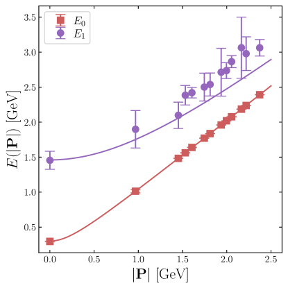
As mentioned in the main text, by employing the spectral decomposition formula along with 2-state or 3-state fits of the pion two-point correlators [62, 70, 71, 72, 73], we extract energy values of both the ground and excited states of the pion, as well as the corresponding amplitudes. We show the results of the ground and the first excited state energy for different momenta in Fig. 12. We can see that the fit results for agree well with the dispersion relation shown by the solid lines, and in most cases, the results for also agree with them within errors.
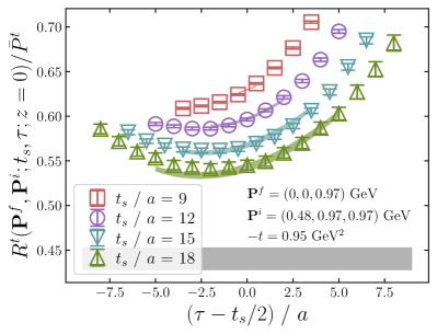
To obtain the matrix elements, we consider the ratio given by Eq. (12) and perform 2-state or 3-state fits. Here, we use the energy levels and amplitudes obtained from the corresponding fits of the two-point functions. In Fig. 13, we select two specific cases from the data of and to show the results of the ratio as . The left one belongs to the case of = 0.97 GeV and = 0.95 GeV2, while the right one corresponds to the case of = 1.94 GeV and = 1.69 GeV2, that is, the largest momentum transfer in this work. The lattice results are shown as the data points with different colors representing the different time separations. The bands with corresponding colors denote the two-state fit results of the lattice data. And the grey bands are the extrapolated results of the ratio, that is, the bare matrix elements. We collect all the bare matrix element results of the largest momentum in Fig. 14. It is evident that the results display a decreasing trend with increasing and also as the momentum transfer increases, as expected.
Appendix B Perturbative coefficient
B.1 Matching coefficient
The NNLO matching kernel with LRR and RGR can be expanded to as [58, 57]
| (23) | ||||
with
| (24) | ||||
Here, the QCD -function
| (25) |
is given by
| (26) | ||||
| (27) | ||||
| (28) |
where , , , and for our lattice ensemble. The 1-loop and 2-loop matching coefficients and are constructed as
| (29) | |||
| (30) |
where represent the normal LL/NLL/NNLL terms, denote the LL/NLL terms in the hybrid scheme. In the last line of Eq. (23), is the LRR term in the hybrid scheme [58, 57]
| (31) | ||||
where is a small exponential decaying factor, , , and means a plus function. Additionally, represents the rest LRR term
| (32) | ||||
where is the generalized exponential integral, denotes the real part, and
| (33) | ||||
with .
B.2 Evolution coefficient
The NNLL matching requires the 3-loop DGLAP evolution kernel, which can be expressed as
| (34) | ||||
where , , is the 1-loop splitting function, and and are the 2-loop and 3-loop splitting functions for the valence quark [81, 82]. They are given by
| (35) | ||||
where the definitions of , , and can be found in Ref. [81]. As for , we take the approximate solution in Eq. (4.23) of Ref. [82].
Note that after the inverse matching, one obtains the matched GPDs at a varying scale in . To implement the DGLAP evolution, we set GeV and and obtain the evolution kernel as a triangular matrix down to a minimal value . Then we invert the triangular matrix and apply it to the matched GPDs , which leads to at the fixed scale down to .
We could also express the evolution kernel as a perturbative series in , but it gives a smaller scale variation as remains small. Instead, we use as a perturbative series in . The latter becomes large at small , which gives us a more conservative estimate of the scale variation uncertainty.