Feature-Specific Coefficients of Determination in Tree Ensembles
Abstract
Tree ensemble methods provide promising predictions with models difficult to interpret. Recent introduction of Shapley values for individualized feature contributions, accompanied with several fast computing algorithms for predicted values, shows intriguing results. However, individualizing coefficients of determination, aka , for each feature is challenged by the underlying quadratic losses, although these coefficients allow us to comparatively assess single feature’s contribution to tree ensembles. Here we propose an efficient algorithm, Q-SHAP, that reduces the computational complexity to polynomial time when calculating Shapley values related to quadratic losses. Our extensive simulation studies demonstrate that this approach not only enhances computational efficiency but also improves estimation accuracy of feature-specific coefficients of determination.
Our proposed Q-SHAP algorithm significantly advances the interpretability of tree ensemble methods by reducing the computational complexity of calculating Shapley values for quadratic losses, such as , to polynomial time. By enabling an efficient and accurate decomposition of , Q-SHAP fosters greater understanding and transparency in machine learning applications, particularly in biomedical fields where model interpretability is paramount. Furthermore, Q-SHAP’s framework has the potential to extend to general loss functions via approximation, opening new avenues for research and broadening its applicability across various machine learning models. This work significantly contributes to making complex models more understandable and trustworthy, enhancing their adoption and impact across diverse domains.
Explainable artificial intelligence (XAI), Shapley values, coeffcients of determination, tree ensembles
1 Introduction
Models built with tree ensembles are powerful but often complicated, making it challenging to understand the influence of inputs. Feature importance plays a critical role in demystifying these models and enhancing their interpretability by assigning each input feature a score. This is crucial in domains like healthcare and biomedicine, where trust and interpretation of the model are essential [1, 2]. Common feature importance measures like gain can be inconsistent [3] while permutation importance lacks theoretical foundations [4].
Shapley values, derived from cooperative game theory and introduced by Shapley [5], offer a robust method for the fair distribution of payoffs generated by a coalition of players. This can be analogously applied to assess the contribution of each feature in a machine learning model. It ensures that each feature’s contribution is assessed by considering all possible combinations of features, thereby providing a comprehensive understanding of feature impacts. Recent applications of Shapley values have focused on local interpretation [6, 3, 7], where they are employed to examine the influence of individual features on specific predictions. Nonetheless, there are numerous scenarios where global importance is preferred, such as analysis of the role of a feature across the entire dataset [8, 9].
Among the works that compute Shapley values in a global context, a popular approach is to use model variance decomposition. Lipovetsky and Conklin [10] decomposed in linear regression, offering consistent interpretations even in the presence of multicollinearity. Owen and Prieur [11] also conducted a conceptual analysis of Shapley values for the variance. However, computation remains a significant challenge, as the calculation of Shapley values grows exponentially with the number of features. To address this issue, several Monte Carlo-based methods have been proposed to effectively reduce the computational burden [12, 9, 13].
Although Monte Carlo-based, model-agnostic methods are more efficient than brute-force approaches, they are still computationally intensive, especially when dealing with high-dimensional data that requires extensive feature permutation sampling to ensure consistency [6, 14]. This challenge has prompted the development of methods that leverage the specific structures of tree-based models. However, much of the focus has been on explaining individual predictions, as seen with TreeSHAP [3], FastTreeSHAP [15], and LinearTreeSHAP [16]. Bénard et al. [17] considered population-level importance using , specifically tailored for random forests [18].
To the best of our knowledge, there is no available method to calculate Shapley values of quadratic losses by leveraging structures of decision trees for fast computation. In this paper, we propose Q-SHAP, which can decompose quadratic terms of predicted values of a decision tree into each feature’s attribute in polynomial time. It leads to fast computation of feature-specific for a decision tree. We also extend our approach to Gradient Boosted Decision Trees.
The rest of the paper is structured as follows. In Section 2, we provide a brief overview of Shapley values of . In Section 3, we present our proposed algorithm Q-SHAP to calculate Shapley values of in polynomial time for single trees, and then extend the approach for tree ensembles in Section 4. We justify the efficacy and efficiency of the algorithm using extensive simulations in Section 5 and real data analysis in high dimension in Section 6. We conclude the paper with a discussion in Section 7.
2 Shapley Values of for Individual Features
2.1 Model specification
Here we investigate a specific label and its explainability by a full set of features . For any subset , we define the corresponding set of features as .
Suppose that, for any set of feature , an oracle model can be built such that, for any specific value ,
The Shapley value of -th feature, in terms of its contribution to the total variation, is defined as
| (1) | |||||
where is the number of features in . The term is the variance explained by feature set and the term is the variance explained solely by set . This definition is analogous to Covert et al. [9] and Williamson and Feng [13]. By averaging over all possible feature combinations, the Shapley values are the only solution that satisfies the desired properties of symmetry, efficiency, additivity, and dummy [5].
Note that can be used to describe the general association of feature with the label . In fact, when a linear model is under consideration with independent features , we have
i.e., measures the scale of Pearson’s correlation between and . Therefore, extends the concept of correlation from a linear model to a general nonlinear model.
2.2 Empirical Estimation
Suppose we have a set of data with sample size observed for both label and features as
Accordingly, we denote the observed data of features in subset as
Suppose that, for each subset of features, a single optimal model is built on data . Then the -th label can be predicted with
2.3 From to a Quadratic Loss
We will establish the connection of to a quadratic loss through equation (1). We define the quadratic loss on the optimal model as
| (2) |
for any set of features . With , we have
Following the law of total variance, we can estimate by
Thus, an empirical estimate of (1) is
which is proportional to a Shapley value for the sum of squared errors, i.e., the quadratic loss in (2).
2.4 From Quadratic Loss to Q-SHAP
We now further reduce Shapley values of the sum of squared errors to Shapley values of linear and quadratic terms of predicted values. Expanding the loss function in (2), we can rewrite,
To calculate this, we define the Shapley value for each sample as,
which is a linear combination of two sets of Shapley values, i.e., Shapley values of predicted value , which are ready to be calculated [3, 15, 16], and Shapley values of the quadratic term of predicted value , i.e.,
| (3) | |||||
for which we will develop the algorithm Q-SHAP to calculate. For the rest of the paper, we will focus on computing the Shapley values in Equation (3) in polynomial time for tree-based models and carrying it over to calculate feature-specific .
3 The Algorithm Q-SHAP for Single Trees
Unlike most regression problems that can yield infinitely many predictions across the diverse input space , decision trees restrict predictions to a finite set, specifically to the values at each leaf node. This nature revitalizes hope in previously unattainable solutions to Shapley values in decision tree-based models. The main idea of our algorithm lies on the fact that Shapley values with various targets such as predictions and various loss functions, are essentially weighted functions of the leaf predictions. While Lundberg et al. [14] suggests that explaining the loss function for a “path-dependent” algorithm is challenging, we provide an exact solution to decomposing quadratic losses using our Q-SHAP. Q-SHAP works for tree ensembles. For simplicity, we here illustrate it with a single decision tree.
3.1 Notations
We assume the underlying decision tree has the maximum depth at and a total of leaves, and use to denote a specific leaf. We further introduce a dot product for polynomials for subsequent calculation. For two polynomials
we define their dot product as
3.2 Distributing the prediction to leaves
Decision trees match each data point to one leaf for prediction. However, for our prediction defined on any subset , a data point can fall into multiple leaves due to the uncertainty by unspecified features . We can calculate , following TreeSHAP, as the empirical mean by aggregating the weighted prediction on each leaf,
| (4) |
where is the weighted prediction from leaf in a tree built on feature set .
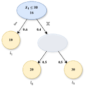
Given an oracle tree built on all available features, we try to recover the oracle tree for a subset of features without rebuilding, following Bifet et al. [16] and Karczmarz et al. [19]. For example, let us take the tree built on two features and as shown in Figure 2. Figure 2 can be viewed as the oracle tree built solely on feature , and hence no longer exists in the tree. Therefore, we replace it with a pseudo internal node to preserve the structure of the original full oracle tree and pave the way for further formulation.
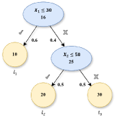
With a data point , we illustrate the calculation in Equation (4) by first calculating the predicted value for the tree in Figure 2,
When the tree is built with an additional feature as shown in Figure 2, we have the predicted value
where the bold numbers reweight for .
Let us take a closer look at these weights, each corresponding to one leaf. For leaf , the weight is 1 since the newly added feature is not involved in its path and the reweighted prediction remains as zero. For leaf , the reweighted prediction is lifted up with the weight inversely proportional to the previous probability because follows its path to the leaf with probability 1. On the other hand, although the path to leaf includes the newly added feature but doesn’t follow this path, resulting in a weight at 0. Next we will generalize such a reweighting strategy to calculate (4) for trees with different sets of features.
Denote the features involved in the path to leaf and the subset of whose decision criteria are satisfied by . Note that each feature may appear multiple times in the path to leaf so we denote the number of samples passing through the node which is attached to the -th appearance. We similarly define for each feature .
For any feature , we can define the weight function based on a partition of into three subsets , , and ,
Therefore, for , we have
Recursive application of the above formula leads to
where with the sample size at leaf , the total sample size, and the predicted value at leaf based on the model built on all features.
When , the above result reduces to
so the optimal prediction is just the mean for all data points, which is consistent with .
We can rewrite (3) as
We further define, for leaves and ,
| (5) | |||||
and we have
Therefore, we will focus on the calculation of in (5) the rest of this section.
We can reduce the calculation of in (5) by only calculating with
because
In combination with the proposition below, computation in (5) can be dramatically reduced from the full feature set to a set only related to the corresponding leaves in a tree.
Proposition 1
For any well-defined ,
We leave the proof of Proposition 1 in Appendix .1. Further denote and a polynomial of ,
We then define a coefficient polynomial
Theorem 1
We further notice that is the coefficient of in polynomial , hence the equation holds with adjusting the weight based on the size of set .
We only need to consider feature as, otherwise, we have following the definition of . Note that, when there is a feature in set that doesn’t belong to , we have
Thus we can further simplify the term to
Consequently, the evaluation of can be reduced to a much smaller set.
3.3 The Algorithm
In this section, we will introduce our algorithms. Theorem 1 demonstrates that we can construct a polynomial form of the NP-problem. Now we introduce a fast and stable evaluation for the dot product of a coefficient polynomial where we know the coefficients and a polynomial with a known product form, involved in Theorem 1.
Proposition 2
Let be a vector of the complex -th roots of unity whose element is for , c the coefficient vector of , and IFFT the Inverse Fast Fourier Transformation. Then
The proof of Proposition 2 is shown in Appendix .1. We facilitate the computation via the complex roots of unity because of their numerical stability and fast operations in matrix multiplications. Due to the potential issue of ill condition, especially at large degrees, our calculation avoids inversion of the Vandermonde matrices, although it has been proposed to facilitate the computing by Bifet et al. [16]. In addition, for each sample size , we only need calculate IFFT once, up to order in operations, and the results can be saved for the rest of calculation through Q-SHAP. Note that term and term in are complex conjugates, and, for a real vector , IFFT also has the conjugate property for paired term and term . Consequently, the dot product of and IFFT inherits the conjugate property and its imaginary parts are canceled upon addition. Therefore, we only need evaluate the dot product at half of the complex roots.
We can aggregate the values of leaf combinations to derive the Shapley values of squared predictions using Q-SHAP as in Algorithm 1 and then calculate the Shapley values of using RSQ-SHAP as in Algorithm 2. The calculation of feature-specific uses the iterative Algorithm 1 instead of a recursive one. The time complexity of the algorithm is for a single tree, which is super fast when the maximum tree depth is not too large.
4 The Algorithm Q-SHAP for Tree Ensembles from Boosting
Tree ensembles from Gradient Boosted Machines (GBM) [20] greatly improve predictive performance by aggregating many weak learners [21, 22, 23]. Each tree, say tree , is constructed on the residuals from the previous tree, i.e., tree . We assume that there are a total of trees in the ensemble and the quadratic loss by the first trees, with all features in , is . Denoting , the -th tree reduces the loss by
with the tree ensemble reducing the total loss by
Per our interest in feature-specific , we resort to the quadratic loss defined as the sum of squared errors in (2).
On the other hand, the -th tree provides the prediction . Therefore, the prediction by the first trees can be recursively calculated as
where is the learning rate and . Note that the residuals after building tree are
which are taken to build the -th tree. Thus,
Therefore, the decomposition of for feature-specific Shapley values in the -th tree is again subject to the decomposition of two sets of values, i.e., both the predicted value and its quadartic term, which can be similarly dealt with the algorithms proposed in the previous section.
5 Simulation Study
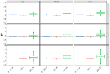
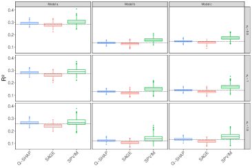
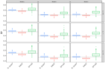
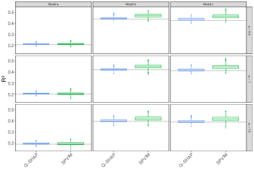
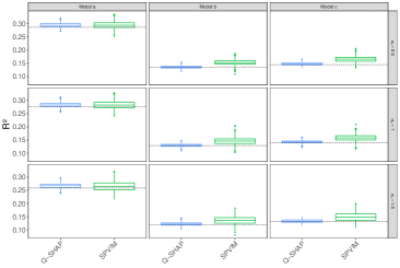
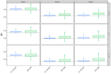
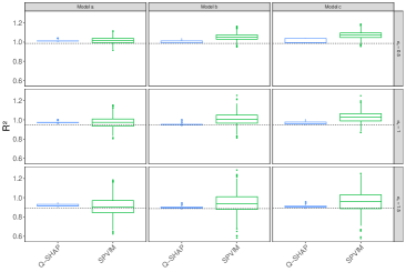
One of the challenges in assessing methods that explain predictions is the typical absence of a definitive ground truth. Therefore, to fairly demonstrate the fidelity of our methodology, we must rely on synthetic data that allows for the calculation of the theoretical Shapley values. Here we consider three different models,
All three features involved in the models are generated from Bernoulli distributions,
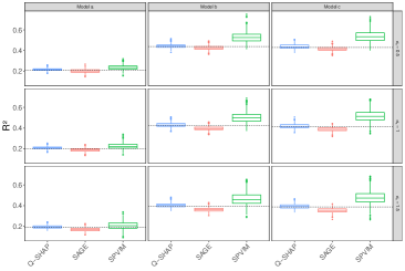
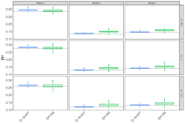
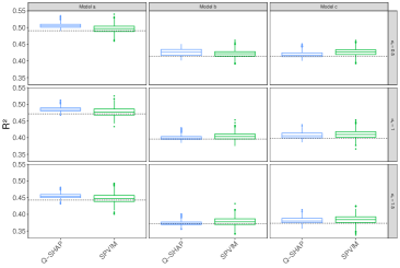
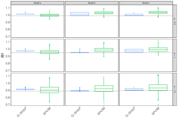
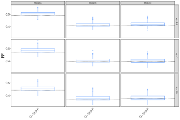
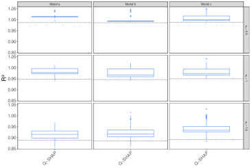
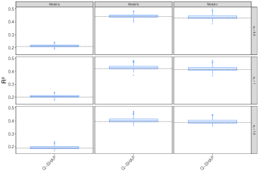
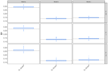
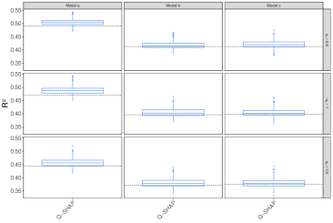
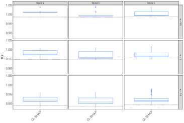
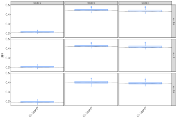
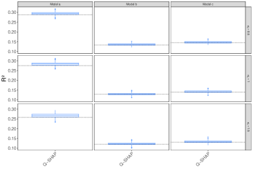
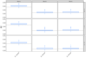
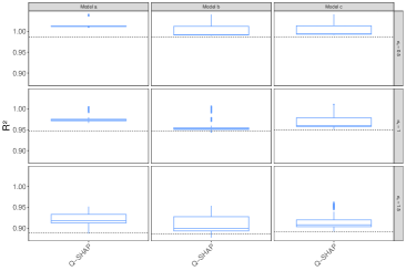
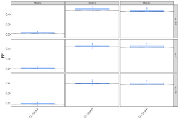
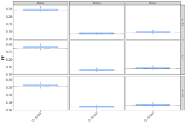
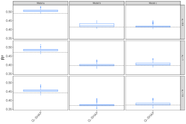
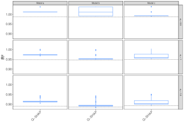
We also simulate additional nuisance features independently from to make the total number of features and , respectively. The error term is generated from with at three different levels, i.e., , , and . The theoretical values of total and feature-specific are shown in Table 1 of Appendix .2 as well as indicated by dashed lines in Figure 3.
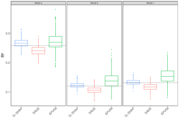
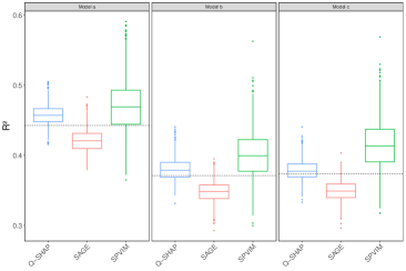
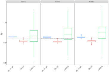
We evaluate the performance of three different methods, our proposed Q-SHAP, SAGE by Covert et al. [9], and SPVIM by Williamson and Feng [13], in calculating the feature-specific for the above three models with data sets of different sample sizes at , and . We use package sage-importance for SAGE and package vimpy for SPVIM to calculate feature-specific Shapley values of total explained variance, which are divided by the total variance for corresponding feature-specific values.
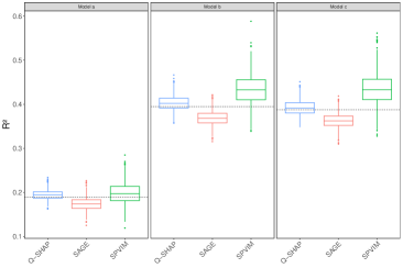
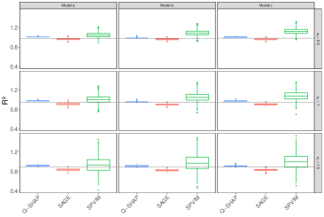
For each setting, we generated 1,000 data sets. For each data set, we built a tree ensemble using XGBoost [21] with tuning parameters optimized via 5-fold cross-validation and grid search in a parameter space specified with the learning rate in and number of estimators in . We fixed the maximum depth of Models a, b, and c at 1, 2, and 3 respectively. Figure 3 show the calculated feature-specific for the first three features as well as the sum of all feature-specific for all three models with , , and . The results of the three models in other settings are shown in Appendix .3. Overall, Q-SHAP provides a more stable and accurate calculation of feature-specific than the other two methods.
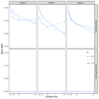
We divide all features into two groups, signal features (the first three) and nuisance features (the rest). For each group, we calculated the mean absolute error (MAE) by comparing feature-specific values to the theoretical ones in each of the 1,000 datasets and averaged MAE over the 1,000 datasets, shown in Figure 4. Note that, by limiting memory to 2GB, SAGE can only report for the data sets with sample size at 500 and 1,000.
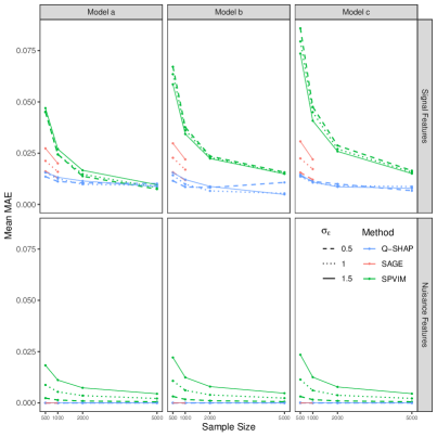
For both signal and nuisance features, Q-SHAP and SAGE exhibit consistent behavior across all models. In contrast, SPVIM tends to bias the calculation, especially for small sample sizes, indicated by the rapid increase of MMAE when the sample size goes down. Among signal features, Q-SHAP has better accuracy than SAGE, followed by SPVIM in general. All methods tend to have better accuracy when sample size increases.
For the nuisance features, only SPVIM is biased away from 0. On the other hand, both Q-SHAP and SAGE have almost no bias for nuisance features across different sample sizes. For all three methods, of signal features tends to have a larger bias than nuisance features.
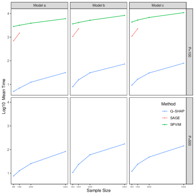
We compared the computational time of the three different methods by running all algorithms in parallel on a full node consisting of two AMD CPUs@2.2GHz with 128 cores and 256 GB memory. We unified the environment with the help of a Singularity container [24] built under Python version 3.11.6. Due to the large size of the simulation, we limit all methods to a maximum wall time of 4 hours per dataset on a single core, with memory limited to 2 GB. The running times are shown in Figure 5. Both SAGE and SPVIM demanded a long time to compute even with only 100 features. Q-SHAP is hundreds of times faster than both SAGE and SPVIM in general and is the only method that can be completed when the dimension is 500 in constrained computation time and memory.
6 Real Data Analysis
We illustrate the utility of Q-SHAP by applying it to predicting Gleason score, a grading prognosis of men with prostate cancer, with gene expressions. The dataset was gerenated by The Cancer Genome Atlas Program (TCGA) [25], including 551 samples and 17,261 features. The Gleason score was retrieved through TCGAbiolinks [26] and further adjusted for age and race as potential confounding factors. The gene expression data was downloaded from UCSC Xena [27] and preprocessed using SIGNET [28].
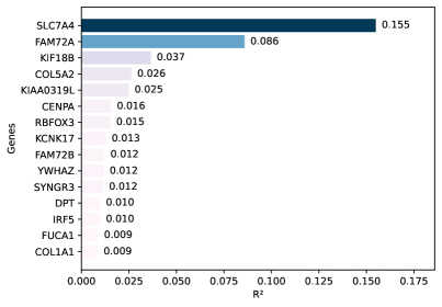
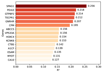
We first constructed the tree ensemble using XGBoost with tuning parameters optimized via 5-fold cross-validation and random research in a parameter space specified with the number of trees in , maximum depth in , and learning rate in . As both SAGE and SPVIM cannot manage this large number of features, we only applied Q-SHAP to the tree ensemble built on 17,261 features, which took 11 minutes to compute and reported the sum of all feature-specific at which is equivalent to the model . The 15 highest feature-specific values are reported in Figure 6.
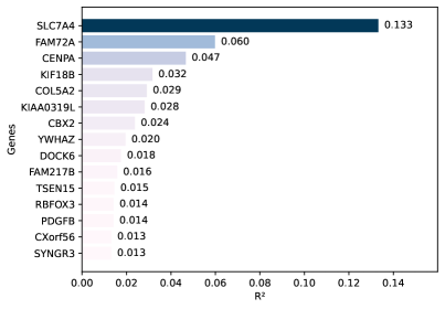
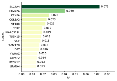
To allow the application of both SAGE and SPVIM, we selected the top 100 features based the result of Q-SHAP, and rebuilt the tree ensemble with the selected 100 features using XGBoost. The rebuilt tree ensemble reported a total of at . Calculating the 100 feature-specific values took about 10 seconds of Q-SHAP, 16 minutes of SAGE, and 67 hours of SPVIM. As shown in Figures 7-9, SPVIM tends to overstate the feature-specific although all of its feature-specific only sums up to 0.72, much lower than 0.93 reported by Q-SHAP. On the other hand, SAGE tends to underestimate the feature-specific and all its feature-specific also sums up to only 0.73, but its top 15 features match well with those by Q-SHAP. In summary, the real data analysis shows consistent results with the simulation study, confirming that Q-SHAP is superior in both computational time and the accuracy of feature-specific .
7 Conclusion
The coefficient of determination, aka , measures the proportion of the total variation explained by available features. Its additive decomposition, following Shapley [5], provides an ideal evaluation of each feature’s attribute to explaining the total variation. However, the calculation of corresponding Shapley values is an NP-hard problem, and further complicated by complexities involved in building tree ensembles. Recently, several methods [3, 15, 16] have been developed to leverage the structure of tree-based models and provide computationally efficient algorithms to decompose the predicted values. However, decomposing demands the decomposition of a quadratic loss reduction by multiple trees. We have shown in Section 4 that we can attribute the total loss reduction by the tree ensemble to each single tree, and the tree-specific loss reductions are subject to further decomposition to each feature. However, decomposing a quadratic loss of a single tree need work with the squared terms of predicted values, invalidating previously developed methods for predicted values. Thus we developed Q-SHAP algorithm to calculate Shapley values of squared terms of predicted values in polynomial time. The algorithm works not only for but also for general quadratic losses. Ultimately, it may provide a framework for more general loss functions via approximation.
Acknowledgment
We gratefully acknowledge the financial support from NIH grant R01GM131491 and NCI Grant R03 CA235363. The results shown in Section 6 are in part based upon data generated by the TCGA Research Network: https://www.cancer.gov/tcga.
References
- Stiglic et al. [2020] G. Stiglic, P. Kocbek, N. Fijacko, M. Zitnik, K. Verbert, and L. Cilar, “Interpretability of machine learning-based prediction models in healthcare,” Wiley Interdisciplinary Reviews: Data Mining and Knowledge Discovery, vol. 10, no. 5, p. e1379, 2020.
- Bussmann et al. [2021] N. Bussmann, P. Giudici, D. Marinelli, and J. Papenbrock, “Explainable machine learning in credit risk management,” Computational Economics, vol. 57, no. 1, pp. 203–216, 2021.
- Lundberg and Lee [2017a] S. M. Lundberg and S.-I. Lee, “Consistent feature attribution for tree ensembles,” Workshop on Human Interpretability in Machine Learning, 2017.
- Ishwaran [2007] H. Ishwaran, “Variable importance in binary regression trees and forests,” Elecctronic Journal of Statistics, vol. 1, pp. 519–537, 2007.
- Shapley [1953] L. S. Shapley, “A value for N-person games,” Contributions to the Theory of Games, vol. 2(28), p. 307–317, 1953.
- Lundberg and Lee [2017b] S. M. Lundberg and S.-I. Lee, “A unified approach to interpreting model predictions,” Advances in Neural Information Processing Systems, vol. 30, 2017.
- Chau et al. [2022] S. L. Chau, R. Hu, J. Gonzalez, and D. Sejdinovic, “RKHS-SHAP: Shapley values for kernel methods,” Advances in Neural Information Processing Systems, vol. 35, pp. 13 050–13 063, 2022.
- Molnar [2020] C. Molnar, Interpretable Machine Learning. lulu.com, 2020.
- Covert et al. [2020] I. Covert, S. M. Lundberg, and S.-I. Lee, “Understanding global feature contributions with additive importance measures,” Advances in Neural Information Processing Systems, vol. 33, pp. 17 212–17 223, 2020.
- Lipovetsky and Conklin [2001] S. Lipovetsky and M. Conklin, “Analysis of regression in game theory approach,” Applied Stochastic Models in Business and Industry, vol. 17, no. 4, pp. 319–330, 2001.
- Owen and Prieur [2017] A. B. Owen and C. Prieur, “On Shapley value for measuring importance of dependent inputs,” SIAM/ASA Journal on Uncertainty Quantification, vol. 5, no. 1, pp. 986–1002, 2017.
- Song et al. [2016] E. Song, B. L. Nelson, and J. Staum, “Shapley effects for global sensitivity analysis: theory and computation,” SIAM/ASA Journal on Uncertainty Quantification, vol. 4, no. 1, pp. 1060–1083, 2016.
- Williamson and Feng [2020] B. Williamson and J. Feng, “Efficient nonparametric statistical inference on population feature importance using Shapley values,” in International Conference on Machine Learning. PMLR, 2020, pp. 10 282–10 291.
- Lundberg et al. [2020] S. M. Lundberg, G. Erion, H. Chen, A. DeGrave, J. M. Prutkin, B. Nair, R. Katz, J. Himmelfarb, N. Bansal, and S.-I. Lee, “From local explanations to global understanding with explainable ai for trees,” Nature Machine Intelligence, vol. 2, no. 1, pp. 56–67, 2020.
- Yang [2021] J. Yang, “Fast Treeshap: Accelerating SHAP value computation for trees,” Advances in Neural Information Processing Systems, vol. 34, 2021.
- Bifet et al. [2022] A. Bifet, J. Read, C. Xu et al., “Linear TreeShap,” Advances in Neural Information Processing Systems, vol. 35, pp. 25 818–25 828, 2022.
- Bénard et al. [2022] C. Bénard, G. Biau, S. Da Veiga, and E. Scornet, “SHAFF: Fast and consistent SHApley eFfect estimates via random Forests,” in International Conference on Artificial Intelligence and Statistics. PMLR, 2022, pp. 5563–5582.
- Breiman [2001] L. Breiman, “Random Forests,” Machine Learning, vol. 45, pp. 5–32, 2001.
- Karczmarz et al. [2022] A. Karczmarz, T. Michalak, A. Mukherjee, P. Sankowski, and P. Wygocki, “Improved Feature Importance Computation for Tree Models based on the Banzhaf Value,” in Proceedings of the Thirty-Eight Conference on Uncertainty in Artificial Intelligence, 2022, pp. 969–979.
- Friedman [2001] J. H. Friedman, “Greedy function approximation: A gradient boosting machine,” Annals of Statistics, pp. 1189–1232, 2001.
- Chen and Guestrin [2016] T. Chen and C. Guestrin, “XGBoost: A scalable tree boosting system,” in Proceedings of the 22nd ACM SIGKDD International Conference on Knowledge Discovery and Data Mining, 2016, pp. 785–794.
- Ke et al. [2017] G. Ke, Q. Meng, T. Finley, T. Wang, W. Chen, W. Ma, Q. Ye, and T.-Y. Liu, “Lightgbm: A highly efficient gradient boosting decision tree,” Advances in Neural Information Processing Systems, vol. 30, 2017.
- Prokhorenkova et al. [2018] L. Prokhorenkova, G. Gusev, A. Vorobev, A. V. Dorogush, and A. Gulin, “Catboost: unbiased boosting with categorical features,” Advances in Neural Information Processing Systems, vol. 31, 2018.
- Kurtzer et al. [2017] G. M. Kurtzer, V. Sochat, and M. W. Bauer, “Singularity: Scientific containers for mobility of compute,” PLOS ONE, vol. 12, no. 5, p. e0177459, 2017.
- Weinstein et al. [2013] J. N. Weinstein, E. A. Collisson, G. B. Mills, K. R. Shaw, B. A. Ozenberger, K. Ellrott, I. Shmulevich, C. Sander, and J. M. Stuart, “The cancer genome atlas pan-cancer analysis project,” Nature Genetics, vol. 45, no. 10, pp. 1113–1120, 2013.
- Colaprico et al. [2016] A. Colaprico, T. C. Silva, C. Olsen, L. Garofano, C. Cava, D. Garolini, T. S. Sabedot, T. M. Malta, S. M. Pagnotta, I. Castiglioni et al., “TCGAbiolinks: an R/Bioconductor package for integrative analysis of TCGA data,” Nucleic Acids Research, vol. 44, no. 8, p. e71, 2016.
- Goldman et al. [2020] M. J. Goldman, B. Craft, M. Hastie, K. Repečka, F. McDade, A. Kamath, A. Banerjee, Y. Luo, D. Rogers, A. N. Brooks et al., “Visualizing and interpreting cancer genomics data via the Xena platform,” Nature Biotechnology, vol. 38, no. 6, pp. 675–678, 2020.
- Jiang et al. [2023] Z. Jiang, C. Chen, Z. Xu, X. Wang, M. Zhang, and D. Zhang, “SIGNET: Transcriptome-wide causal inference for gene regulatory networks,” Scientific Reports, vol. 13, no. 1, p. 19371, 2023.
- Gould [1972] H. W. Gould, Combinatorial Identities. Morgantown Printing and Binding Co, 1972.
- Geddes et al. [1992] K. O. Geddes, S. R. Czapor, and G. Labahn, Algorithms for Computer Algebra. Springer Science & Business Media, 1992.
.1 Proofs
We first establish the following lemma.
Lemma 1
Proof. Using Gould’s identity [29], we have
where we used the Hockey-Stick Identity in the last step.
Proof of Proposition 2. We first rewrite the two polynomials
where is the Vandermonde matrix for vector , and and are the coefficients of polynomials and , respectively. Then the inner product
Letting
and noting that the Vandermonde matrix evaluated at is symmetric, we have
whose multiplication with is just the Inverse Fast Fourier transformation (IFFT) over [30]. Hence the proposition holds.
.2 Calculation of Theoretical Shapley Values of
Here we will calculate the theoretical feature-specific values of the following three models,
With all three features generated from Bernoulli distribution, we have
For Model a, we have
For Model b, we have
For Model c, we have
For all of the cases the Shapley values can be calculated as
Therefore, the theoretical feature-specific in the three models can be evaluated and are shown in Table 1.
| Model | Total | ||||
|---|---|---|---|---|---|
| 0.50 | 0.9864 | 0.2094 | 0.2863 | 0.4907 | |
| a | 1.00 | 0.9477 | 0.2012 | 0.2750 | 0.4715 |
| 1.50 | 0.8894 | 0.1888 | 0.2581 | 0.4425 | |
| 0.50 | 0.9860 | 0.4390 | 0.1341 | 0.4129 | |
| b | 1.00 | 0.9459 | 0.4212 | 0.1286 | 0.3961 |
| 1.50 | 0.8860 | 0.3945 | 0.1205 | 0.3710 | |
| 0.50 | 0.9868 | 0.4288 | 0.1450 | 0.4130 | |
| c | 1.00 | 0.9491 | 0.4124 | 0.1395 | 0.3972 |
| 1.50 | 0.8925 | 0.3878 | 0.1312 | 0.3735 | |
.3 Boxplots of the First Three Feature-Specific and Total Values
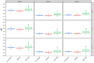
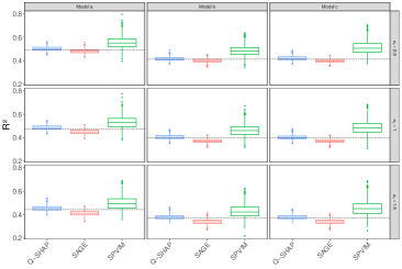
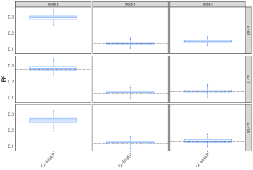
We have compare the preformance of three different methods, i.e., our proposed Q-SHAP, SAGE by Covert et al. [9], and SPVIM by Williamson and Feng [13], in calculating the feature-specific as well as the sum of all feature-specific for the three models specified in Section 5, with different settings, i.e., , , and . The results are shown in Fig. 10-17. Note that the results of SAGE are unavailable in Fig. 12-17 because it cannot report those with our limited computational resources, and the results of SPVIM are unavailable in Fig. 14-17 because it demands too much time to complete the computation when .


.4 Plots of the mean absolute error (MAE)
Similar to Fig. 4, we show in Fig. 18 the mean absolute error (MAE) of feature-specific for both signal and nuisance features averaged over 1,000 datasets when . Note that the results of SAGE and SPVIM are unavailable because none of them can complete the computation for with the limited computational resources.