Polarons in supersolids:
path-integral treatment of an impurity in a one-dimensional dipolar supersolid

Abstract

The supersolid phase of a dipolar Bose-Einstein condensate has an intriguing excitation spectrum displaying a band structure. Here, the dressing of an impurity in a one-dimensional dipolar supersolid with the excitations of the supersolid is studied. The ground-state energy of the supersolid polaron is calculated using a variational path integral approach, which obtained accurate results for other polaron systems within the Bogoliubov and Fröhlich approximations. A divergence is observed at the superfluid-supersolid phase transition. The polaron radius is also computed, showing that for strong impurity-atom interactions, the polaron can become localized to a single droplet, behaving like a small solid-state polaron.

I Introduction

A supersolid is a state of matter that exhibits at the same time properties of a superfluid, such as frictionless flow, and properties of a solid, such as periodic density modulations unrelated to external potentials [1, 2, 3, 4, 5]. There are three main features associated with supersolidity: spontaneously arising periodic density modulations, global phase coherence (due to the superfluid fraction of the supersolid), and phase rigidity [5]. Solid helium has been a candidate system for supersolidity. However, early experimental claims of supersolidity in solid helium [6] were later disproved [7], and no new evidence has emerged at the time of writing [1, 5, 8]. Recently, supersolidity has been observed in ultracold gases such as spin-orbit-coupled Bose-Einstein condensates (BECs) and dipolar BECs [8, 5, 9, 1, 10]. The dipolar supersolid realization is of great interest as the supersolidity comes from the intrinsic dipole-dipole interactions and is not due to, for example, a superimposed optical lattice. Different systems and properties of dipolar supersolids have been studied recently, such as vortices, excitations, and its superfluid fraction [11, 12, 2, 13]. However, the effect of an impurity has yet to be studied in the context of a dipolar supersolid. The problem of an impurity in a Bose-Einstein condensate has been studied extensively for superfluid contact and dipolar Bose gases [14, 15, 16, 17, 18, 19, 20, 21, 22, 23, 24, 25, 26, 27, 28, 29]. The polaron effect, where the impurity gets dressed by the excitations of the system, is particularly interesting as in the supersolid regime the excitation spectrum displays a band structure with two Goldstone phonon modes compared to the single phonon mode of a superfluid Bose gas [2].

This paper studies the dressing of a neutral impurity, which can have a finite magnetic moment, with the excitations of a one-dimensional dipolar supersolid. The polaronic energy is calculated within the Fröhlich and Bogoliubov approximations suited for weak impurity-atom and atom-atom interactions. The variational Feynman path-integral method is used, which has been shown to give results comparable to Monte Carlo methods while being numerically less intensive and time-consuming for other polaron problems [21, 25, 30]. The effect of different system parameters on the polaronic energy is studied. A divergence in the polaronic energy is observed when crossing into the supersolid region, which can be another indication of supersolidity experimentally. The radius of the polaron is calculated, and it is found that for specific values, the polaron becomes localized to a single droplet of the supersolid and behaves like a small solid-state polaron, hopping from one droplet to another.

The paper is organized as follows. In Section II, the Hamiltonian describing the supersolid polaron is derived within the Bogoliubov and Fröhlich approximations. Section III discusses the description of the one-dimensional dipolar supersolid itself. The wavefunction is calculated, and the Bogoliubov-de Gennes equation is solved to obtain the excitations. The polaronic energy and polaron radius are calculated in Section IV using the variational path-integral method, and the results are discussed. The conclusion and outlook are given in the last section, Section V.

II Polaron Hamiltonian in the supersolid regime

The Hamiltonian describing an impurity with mass $m_{I}$ in a one-dimensional dipolar Bose gas is given by

$$\hat{H} =\frac{\hat{p}_{I}^{2}}{2m_{I}}+\sum_{q}\left(\frac{\hbar^{2}q^{2}}{2m_{B}}-\mu+E_{t}\right)\hat{a}^{\dagger}_{q}\hat{a}_{q}$$

$$+\frac{1}{2L}\sum_{k,k^{\prime},q}V(q)\hat{a}^{\dagger}_{k^{\prime}-q}\hat{a}^{\dagger}_{k+q}\hat{a}_{k}\hat{a}_{k^{\prime}}$$

$$+\frac{1}{L}\sum_{k,q}V_{IB}(q)\hat{\rho}_{I}(q)\hat{a}^{\dagger}_{k-q}\hat{a}_{k}.$$ (1)

The first two terms represent the free impurity and a gas of non-interacting bosons, respectively, where $\hat{a}^{\dagger}_{q}$ and $\hat{a}_{q}$ are the creation and annihilation operators of a dipolar atom of mass $m_{B}$ with momentum $q$, $\mu$ is the chemical potential, and $E_{t}$ is the contribution of the transverse confinement to the energy. The third term represents the interaction between the dipolar atoms characterized by an interaction amplitude given by the effective one-dimensional dipolar interaction potential in momentum space $V(q)$. The interaction between the impurity and the bosons is described by the last term, where $\hat{\rho}_{I}(q)=\exp(iq\hat{z}_{I})$ is the impurity density and $V_{IB}(q)$ is the Fourier transform of the impurity-atom interaction potential. The one-dimensional dipolar Bose gas is formed by tightly confining the condensate in the $x$ and $y$ directions using a harmonic trap with oscillator length $l_{\perp}$. The transverse degrees of freedom can be integrated out by using the following ansatz [31, 32]

$$\psi_{\perp}(x,y)=\frac{1}{\sqrt{\pi}\sigma l_{\perp}}\exp\left(-\frac{\nu x^{2}+y^{2}/\nu}{2(\sigma l_{\perp})^{2}}\right).$$ (2)

$\sigma$ and $\nu$ are variational parameters that can be obtained by minimizing the energy of the condensate. $E_{t}=\hbar^{2}(1/\nu+\nu)(1/\sigma^{2}+\sigma^{2})/(4m_{B}l_{\perp})$ is the transverse trap energy corresponding to the above transverse wavefunction[31, 32]. There is no analytical form for the Fourier transform of the effective one-dimensional dipolar interaction potential. Nonetheless, it has been shown that it can be described well by the following analytical expression [31, 32]

$$V(q)=g_{1D}^{(B)}\left(1+\epsilon^{(B)}_{dd}\left(\frac{3\left(1+Qe^{Q}\text{Ei}(-Q)\right)}{1+\nu}-1\right)\right),$$ (3)

with $g_{1D}^{(B)}=2\hbar^{2}a^{(B)}_{s}/(m_{B}\sigma^{2}l_{\perp}^{2})$ the 1D s-wave interaction strength of the dipolar bosons and $a^{(B)}_{s}$ the s-wave scattering length of the dipolar bosons. The strength of the dipole-dipole interaction is characterized by $\epsilon^{(B)}_{dd}=\mu_{0}\mu_{B}^{2}m_{B}/(12\pi\hbar^{2}a^{(B)}_{s})$ where $\mu_{0}$ is the vacuum permeability, and $\mu_{B}$ is the dipole moment of the atoms, $Q=\sqrt{\nu}(q\sigma l_{\perp})^{2}/2$, and $\text{Ei}(Q)$ the exponential integral.

The impurity-atom interaction potential in momentum space, $V_{IB}(q)$, has the same form as $V(q)$, expression (3), but with $g_{1D}^{(B)}$ and $\epsilon^{(B)}_{dd}$ replaced by their impurity-boson counterparts $g_{1D}^{(IB)}$ and $\epsilon^{(IB)}_{dd}$, respectively. In particular, $g_{1D}^{(IB)}=\hbar^{2}a^{(IB)}_{s}/(m_{r}\sigma^{2}l_{\perp}^{2})$ is the 1D s-wave interaction strength of the dipolar boson-impurity interaction, $a^{(IB)}_{s}$ the s-wave scattering length for the impurity-atom interactions, $\epsilon^{(IB)}_{dd}=\mu_{0}\mu_{I}\mu_{B}m_{r}/(6\pi\hbar^{2}a^{(IB)}_{s})$ where $\mu_{I}$ is the impurity dipole moment, and $m_{r}=(m_{B}^{-1}+m_{I}^{-1})^{-1}$ the reduced mass.

In the supersolid regime where there is a density modulation, the ground state wavefunction of the dipolar gas is no longer given by the constant $\sqrt{n}$ but can be described by [31]

$$\psi_{0}(z)=\sqrt{n_{0}}\left(1+\sum_{l=1}^{\infty}\Delta_{l}\cos(lk_{s}z)\right),$$ (4)

with $n_{0}=N_{0}/L$ the density of atoms in the zero-momentum mode, $k_{s}$ the momentum characterizing the density modulation, and the order parameters $\Delta_{l}$ describing the contribution of mode $l$ to the wavefunction. As translational symmetry is broken, a dipolar atom of the supersolid can be described by $q$, which is restricted to the first Brillouin zone (BZ) given by $[-k_{s}/2,k_{s}/2]$ and an integer $l$ [31]. The momentum of the atom is then given by $q+lk_{s}$. The Hamiltonian becomes

$$\hat{H} =\frac{\hat{p}_{I}^{2}}{2m_{I}}+\sum_{q,l}\left(\frac{\hbar^{2}(q+lk_{s})^{2}}{2m_{B}}-\mu+E_{t}\right)\hat{a}^{\dagger}_{q,l}\hat{a}_{q,l}$$

$$+\frac{1}{2L}\sum_{k,k^{\prime},q,l,m,s}V(q+sk_{s})\hat{a}^{\dagger}_{k^{\prime}-q,m-s}\hat{a}^{\dagger}_{k+q,l+s}\hat{a}_{k,l}\hat{a}_{k^{\prime},m}$$

$$+\frac{1}{L}\sum_{k,q,l,l^{\prime}}V_{IB}(q+lk_{s})\hat{\rho}_{I}(q+lk_{s})\hat{a}^{\dagger}_{k-q,l^{\prime}-l}\hat{a}_{k,l^{\prime}}.$$ (5)

Here, $\hat{a}^{\dagger}_{q,l}$ and $\hat{a}_{q,l}$ are the creation and annihilation operators of a dipolar atom of mass $m_{B}$ with momentum $q$ in mode $l$. Similarly to the case of a neutral [18] and charged [33] impurity in a Bose gas, the Bogoliubov approximation and transformation can be applied. However, because of the broken translational symmetry, other modes with momentum $q=lk_{s}$ apart from the zero-momentum mode are also macroscopically occupied [31]. The Bogoliubov approximation is now given by $\hat{a}_{0,l}\rightarrow\Delta_{l}\sqrt{N_{0}}/2$ with $\Delta_{0}=2$ and $\Delta_{-l}=\Delta_{l}$ [31]. A Bogoliubov transformation

$$\hat{a}_{q,l}=\sum_{l^{\prime}}u^{l^{\prime}}_{l}(q)\hat{\alpha}_{q,l^{\prime}}+v^{l^{\prime}}_{l}(q)\hat{\alpha}^{\dagger}_{-q,l^{\prime}},$$ (6)

can be found such that the supersolid term of the Hamiltonian diagonalizes with $u^{l^{\prime}}_{l},v^{l^{\prime}}_{l}$ the Bogoliubov coefficients and $\hat{\alpha}^{\dagger}_{q,l},\hat{\alpha}_{q,l}$ the Bogoliubov creation and annihilation operators of a dipolar boson with momentum $q$ in mode $l$. The Bogoliubov coefficients are normalized by the following relation, which is derived by enforcing the bosonic commutation relation

$$\sum_{l^{\prime}}[(u_{l}^{l^{\prime}}(q))^{2}-(v_{l}^{l^{\prime}}(q))^{2}]=1.$$ (7)

Applying it to the Hamiltonian results in

$$\hat{H}= \frac{\hat{p}_{I}^{2}}{2m_{I}}+\sum_{q,l}\epsilon_{l}(q)\hat{\alpha}^{\dagger}_{q,l}\hat{\alpha}_{q,l}+U(\hat{z_{I}})$$

$$+\sum_{q,l}V_{l}(q,\hat{z_{I}})\left(\hat{\alpha}_{q,l}+\hat{\alpha}^{\dagger}_{-q,l}\right),$$ (8)

where

$$V_{l}(q,\hat{z}_{I})= \frac{\sqrt{N_{0}}}{2L}\sum_{m,m^{\prime}}V_{IB}(q+mk_{s})e^{i(q+mk_{s})\hat{z}_{I}}$$

$$\times\Delta_{m^{\prime}}\left(u^{l}_{m-m^{\prime}}(q)+v^{l}_{m-m^{\prime}}(q))\right),$$ (9)

and

$$U(\hat{z}_{I})=\frac{n_{0}}{4}\sum_{l,l^{\prime}}V_{IB}(lk_{s})\Delta_{l^{\prime}-l}\Delta_{l^{\prime}}e^{ilk_{s}\hat{z}_{I}}.$$ (10)

This is the Hamiltonian describing an impurity in a one-dimensional dipolar supersolid within the Bogoliubov and Fröhlich approximation. Terms with two creation and/or annihilation operators, beyond-Fröhlich terms characterizing the absorption and emission of two Bogoliubov excitations, are neglected and out of scope for this paper. Compared to the neutral and charged Bose polaron problems, the term without any creation or annihilation operators is not constant and acts as an external periodic potential on the impurity. Therefore, it cannot be discarded and will be denoted by $U(z_{I})$ from now on. The problem of an impurity in a dipolar supersolid has been reduced to an impurity interacting with multiple excitation bands via a Fröhlich-like vertex in a periodic background potential $U(z_{I})$. The order parameters will be calculated in the next section, and the Bogoliubov-de Gennes eigenproblem will be solved.

III Supersolid wavefunction and excitations, without impurity

To calculate the wavefunction and order parameters, the total energy of the supersolid needs to be minimized. The (extended) Gross-Pitaevskii energy can be used as an energy functional, which is given by [31]

$$E_{GP}[\psi] =-\int dz\psi^{*}(z)\frac{\hbar^{2}}{2m_{B}}\frac{d^{2}}{dz^{2}}\psi(z)+NE_{t}$$

$$+\frac{1}{2}\int dz\int dz^{\prime}V(z-z^{\prime})|\psi(z)|^{2}|\psi(z^{\prime})|^{2}$$

$$+\frac{2}{5}\gamma\int dz|\psi(z)|^{5}.$$ (11)

The first line is the kinetic energy and the transverse trap energy, while the second and third lines are the dipolar interaction energy and Lee-Huang-Yang (LHY) beyond-mean-field contribution, respectively. The parameter $\gamma$ quantifies the LHY correction and is given by [31, 34]

$$\gamma=\frac{256}{15\pi}\frac{\hbar^{2}(a_{s}^{(B)})^{5/2}}{m_{B}(\sigma l_{\perp})^{3}}\int_{0}^{1}du(1-\epsilon_{dd}^{(B)}+3\epsilon_{dd}^{(B)}u^{2})^{5/2}.$$ (12)

The LHY contribution is taken into account as it prevents collapse and is essential to describe the supersolid state. Using the ansatz (4) results in an expression for the energy in terms of the order parameters $\Delta_{l}$ and the variational parameters $\sigma$ and $\nu$. To obtain an analytical expression for the LHY contribution to the energy, it is assumed that the wavefunction is always positive or zero:

$$1-\sum_{l=1}^{\infty}\Delta_{l}\geq 0,$$ (13)

such that the absolute value can be discarded. This is valid close to the superfluid-supersolid transition. The energy divided by the number of atoms $N$ is given by

$$\frac{E_{GP}[\Delta_{l},k_{s},\sigma,\nu]}{N}=\frac{\hbar^{2}k_{s}^{2}}{4m_{B}}\frac{\sum_{l=1}^{\infty}l^{2}\Delta_{l}^{2}}{1+\sum_{l=1}^{\infty}\Delta_{l}^{2}/2}+E_{t}$$

$$+\frac{n}{32}\frac{\sum_{l,m,p=-\infty}^{\infty}\Delta_{l}\Delta_{m}\Delta_{p}\Delta_{l+m+p}V[(l+m)k_{s}]}{(1+\sum_{l=1}^{\infty}\Delta_{l}^{2}/2)^{2}}$$

$$+\frac{\gamma n^{3/2}}{80}\frac{\sum_{l,m,p,s=-\infty}^{\infty}\Delta_{l}\Delta_{m}\Delta_{p}\Delta_{s}\Delta_{l+m+p+s}}{(1+\sum_{l=1}^{\infty}\Delta_{l}^{2}/2)^{5/2}}.$$ (14)

The above expression can be minimized numerically for $\Delta_{l}$, $k_{s}$, $\sigma$, and $\nu$, which can be substitued into (4) to obtain the ground-state wavefunction of the supersolid.

The excitation spectrum and Bogoliubov coefficients can be obtained by expanding the supersolid part of the Hamiltonian up to second order in creation and annihilation operators. The LHY contribution can be taken into account by using the following Hamiltonian, which results in the correct speed of sound and energy correction [31]

$$\hat{H}_{LHY}=\frac{2}{5}\gamma\int dz\left(\hat{\psi}^{\dagger}(z)\hat{\psi}^{\dagger}(z)\hat{\psi}(z)\hat{\psi}(z)\right)^{5/4},$$ (15)

with

$$\hat{\psi}(z)=\psi_{0}(z)+\frac{1}{\sqrt{L}}\sum_{q\neq 0,l}e^{i(q+lk_{s})z}\hat{a}_{q,l}.$$ (16)

The resulting quadratic Hamiltonian can be written as

$$\hat{H}_{B}= \sum_{q,l,m}\left(h_{q,l,m}\hat{a}^{\dagger}_{q,l}\hat{a}_{q,m}+\frac{1}{2}g_{q,l,m}\hat{a}^{\dagger}_{q,l}\hat{a}^{\dagger}_{-q,m}\right.$$

$$\left.+\frac{1}{2}g_{q,l,m}\hat{a}_{-q,m}\hat{a}_{q,l}\right),$$ (17)

with

$$h_{q,l,m}= \left(\frac{\hbar^{2}(q+lk_{s})^{2}}{2m}-\mu+E_{t}\right)\delta_{l,m}$$

$$+\frac{n_{0}}{4}\sum_{s}V(q+sk_{s})\Delta_{m-s}\Delta_{l-s}$$

$$+\frac{n_{0}}{4}\sum_{s}V((m-l)k_{s})\Delta_{s}\Delta_{s-(l-m)}$$

$$+\frac{5}{2}\gamma n_{0}^{3/2}\sum_{s,s^{\prime}}\frac{\Delta_{s}\Delta_{s^{\prime}}\Delta_{l-m+s+s^{\prime}}}{8},$$ (18)

and

$$g_{q,l,m}= \frac{n_{0}}{4}\sum_{s}V(q+sk_{s})\Delta_{m+s}\Delta_{l-s}$$

$$+\frac{3}{2}\gamma n_{0}^{3/2}\sum_{s,s^{\prime}}\frac{\Delta_{s}\Delta_{s^{\prime}}\Delta_{l+m+s+s^{\prime}}}{8}.$$ (19)

The Bogoliubov-de Gennes eigenproblem is then given by

$$\begin{pmatrix}h_{q}&g_{q}\\ -g_{q}^{T}&-h_{-q}^{T}\end{pmatrix}\begin{pmatrix}u\\ v\end{pmatrix}=\hbar\omega_{q,l}\begin{pmatrix}u\\ v\end{pmatrix}.$$ (20)

Solving the above eigenproblem results in the excitation spectrum and Bogoliubov coefficients for the dipolar supersolid. In Figure 1, the excitation spectrum of a one-dimensional dipolar supersolid is shown for realistic parameters $n=2386.2/l_{\perp}$ and $a^{(B)}_{s}=0.005l_{\perp}$ (which are taken from Ref. [31]) for different dipolar interaction strengths $\epsilon_{dd}^{(B)}$. In this case, the critical value of $\epsilon_{dd}^{(B)}$ is approximately $1.340$. For $\epsilon_{dd}^{(B)}<\epsilon_{dd,c}^{(B)}$, the excitation spectrum is the same as the analytical Bogoliubov dispersion, and a roton minimum is visible, as expected. If $\epsilon_{dd}^{(B)}$ becomes larger than the critical value, a band structure appears with two phononic modes: a crystal phonon mode and a superfluid phonon mode. The larger $\epsilon_{dd}^{(B)}$ becomes, the smaller the superfluid phonon mode becomes until the independent droplet regime is reached, where only the crystal phonon mode remains. For the values shown, the supersolid can be described by three order parameters $\Delta_{1}$, $\Delta_{2}$, and $\Delta_{3}$, and the condition (13) is fulfilled.

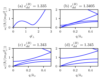
Figure 1: The excitation spectrum of a one-dimensional dipolar supersolid with parameters $n=2386.2$ and $a_{s}^{(B)}=0.005$ in units of $\hbar=m_{B}=l_{\perp}=1$ for different values of $\epsilon^{(B)}_{dd}$. The critical value is given by $\epsilon^{(B)}_{dd,c}=1.34$. The results are equivalent to the ones from Refs. [31, 35].

IV Polaronic energy and polaron radius

For a system with action $S$, an upper bound on the free energy can be found by introducing an exactly solvable variational trial action $S_{0}$ and minimizing for the variational parameters. It is given by the Feynman-Jensen inequality

$$F\leq F_{0}+\frac{1}{\hbar\beta}\langle S-S_{0}\rangle_{0},$$ (21)

where $F_{0}$ is the free energy of the trial action and $\beta=1/(k_{B}T)$ the inverse temperature. For the trial action, a general exactly solvable quadratic trial action is used, which was also applied to other polaron problems and gave results comparable to numerically exact Monte Carlo methods (within the Fröhlich and Bogoliubov approximations) [36, 30],

$$S_{0}=\int\limits_{0}^{\hbar\beta}\frac{m_{I}}{2}\dot{\mathbf{r}}^{2}(\tau)d\tau+\frac{m_{I}}{2\hbar\beta}\int\limits_{0}^{\hbar\beta}\int\limits_{0}^{\hbar\beta}x(\tau-\sigma)\mathbf{r}(\tau)\cdot\mathbf{r}(\sigma)d\tau d\sigma.$$ (22)

Here $x(\tau-\sigma)$ is a variational memory kernel [36, 30]. The kernel statisfies two conditions: it is imaginary-time periodic $x(\hbar\beta-\tau)=x(\tau)$ and $\int_{0}^{\hbar\beta}x(\tau)d\tau=0$ [30]. The free energy and expectation value of the trial action can be found in Ref. [30].

An imaginary-time action corresponding to Hamiltonian (8) can be derived similarly as for the Bose polaron problem [18], and the phonon degrees of freedom can be integrated out as it is the path integral of a forced harmonic oscillator. The resulting effective action is

$$S= \int_{0}^{\hbar\beta}\left(\frac{m_{I}}{2}\dot{z}_{I}(\tau)^{2}+U(z_{I}(\tau))\right)d\tau$$

$$-\frac{1}{\hbar}\sum_{q,l}\int_{0}^{\hbar\beta}d\tau\int_{0}^{\hbar\beta}d\sigma\frac{\cosh(\omega_{q,l}(\hbar\beta/2-|\tau-\sigma|))}{\cosh(\omega_{q,l}\hbar\beta/2)}$$

$$\times V^{*}_{l}(q,z_{I}(\tau))V_{l}(q,z_{I}(\sigma)).$$ (23)

Using the Feynman-Jensen inequality, an upper bound is found for the free energy depending on the kernel used in the trial action $x(\nu)$. An equation for the kernel can be derived by taking the functional derivative of the free energy with respect to the kernel, and putting it equal to zero. The free energy can then be calculated iteratively numerically. The set of equations are

$$F \leq\frac{\hbar}{2\pi}\int_{0}^{\infty}d\nu\left(\log\left(1+\frac{x(\nu)}{\nu^{2}}\right)-\frac{x(\nu)}{x(\nu)+\nu^{2}}\right)+\frac{n_{0}}{4}\sum_{l,l^{\prime}}V_{IB}(lk_{s})\Delta_{l-l^{\prime}}\Delta_{l^{\prime}}\exp\left(-\frac{\hbar l^{2}k_{s}^{2}}{2m_{I}\pi}\int_{0}^{\infty}d\nu\frac{1}{x(\nu)+\nu^{2}}\right)$$

$$-\frac{n_{0}}{4\pi\hbar}\int_{0}^{k_{s}/2}dq\sum_{l,m,m^{\prime},s,s^{\prime}}V_{IB}(q+mk_{s})V_{IB}(q+sk_{s})\Delta_{m^{\prime}}\Delta_{s^{\prime}}(u^{l}_{m-m^{\prime}}(q)+v^{l}_{m-m^{\prime}}(q))(u^{l}_{s-s^{\prime}}(q)+v^{l}_{s-s^{\prime}}(q))$$

$$\int_{0}^{\infty}du\exp\left(-\omega_{q,l}u-\frac{\hbar}{2m_{I}\pi}\int_{0}^{\infty}\frac{d\nu}{x(\nu)+\nu^{2}}((q+mk_{s})^{2}+(q+sk_{s})^{2}-2(q+mk_{s})(q+sk_{s})\cos(\nu u))\right),$$ (24)

and

$$x(\nu) =-\frac{n_{0}k_{s}^{2}}{4m_{I}}\sum_{l,l^{\prime}}l^{2}V_{IB}(lk_{s})\Delta_{l-l^{\prime}}\Delta_{l^{\prime}}\exp\left(-\frac{\hbar l^{2}k_{s}^{2}}{2m_{I}\pi}\int_{0}^{\infty}d\nu\frac{1}{x(\nu)+\nu^{2}}\right)+\frac{n_{0}}{4\pi\hbar m_{I}}\int_{0}^{k_{s}/2}dq\sum_{l,m,m^{\prime},s,s^{\prime}}V_{IB}(q+mk_{s})$$

$$V_{IB}(q+sk_{s})\Delta_{m^{\prime}}\Delta_{s^{\prime}}(u^{l}_{m-m^{\prime}}(q)+v^{l}_{m-m^{\prime}}(q))(u^{l}_{s-s^{\prime}}(q)+v^{l}_{s-s^{\prime}}(q))\int_{0}^{\infty}du((q+mk_{s})^{2}+(q+sk_{s})^{2}-2(q+mk_{s})$$

$$(q+sk_{s})\cos(\nu u))\exp\left(-\omega_{q,l}u-\frac{\hbar}{2m_{I}\pi}\int_{0}^{\infty}\frac{d\nu}{x(\nu)+\nu^{2}}((q+mk_{s})^{2}+(q+sk_{s})^{2}-2(q+mk_{s})(q+sk_{s})\cos(\nu u))\right).$$ (25)

The iterative procedure is started using the Lee-Low-Pines kernel given by $x(\nu)=0$. We consider the upper bound to be converged if the difference with the last value is less than $0.1\%$. A Gauss-Legendre quadrature with $20$ points with $100$ subintervals was used as in Refs. [36, 33] for the polaronic energy calculation. The polaronic energy $F-nV_{IB}(0)$ for $n=2386.2/l_{\perp}$, $a^{(B)}_{s}=0.005l_{\perp}$, $a^{(IB)}_{s}=0.007l_{\perp}$, and $m_{I}=m_{B}$ across the transition as a function of $\epsilon^{(B)}_{dd}-\epsilon^{(B)}_{dd,c}$ is shown in Figure 2. The blue line is for $\epsilon^{(IB)}_{dd}=0$ where the impurity does not have a magnetic moment and is not dipolar. In the superfluid regime, the energy decreases as the system gets closer to the phase transition. There is a divergence visible at the transition $\epsilon^{(B)}_{dd}=\epsilon^{(B)}_{dd,c}$ which was also seen in [26] using the Lee-Low-Pines method in the superfluid regime for a two-dimensional dipolar gas. The divergence from the superfluid regime is driven by the softening of the roton mode [26], while the divergence coming from the supersolid regime is driven by the lowering of the first excitation band. This can be seen by studying the contribution of the different modes $l$ to the ground-state energy. For the values used here, the contribution of the periodic background potential to the ground-state energy is zero except for the mean-field energy contribution $nV_{IB}(0)$. In the supersolid regime, the energy increases as the first excitation band and others become larger. The green dash-dotted line shows the polaronic energy when the impurity is dipolar and has a finite magnetic moment resulting in $\epsilon^{(IB)}_{dd}=0.1$. The additional dipole-dipole interaction for the impurity decreases the impurity-atom interaction potential resulting in an increase of the polaronic energy and a weaker polaron. In Figure 3, the dependence of the polaronic energy on the s-wave scattering length $a^{(IB)}_{s}$ in the supersolid regime is shown for $n=2386.2/l_{\perp}$, $a^{(B)}_{s}=0.005l_{\perp}$, $m_{I}=m_{B}$, $\epsilon^{(B)}_{dd}=1.345$, and $\epsilon^{(IB)}_{dd}=0$ or $0.1$. Similar to the charged Bose polaron problem [33], the energy is always negative and decreases as $a^{(IB)}_{s}$ increases. Even when the impurity has a finite magnetic moment, which increases the polaronic energy, the polaronic energy is always negative within the Fröhlich approximation used here. In the supersolid regime, it can be possible that for strong interaction strengths, the polaron becomes localized to a single droplet (or single “lattice point”) of the supersolid. To study the localization of the polaron, the polaron radius needs to be calculated. The polaron radius can be calculated using [37, 33]

$$r_{p}=\sqrt{\frac{\pi\hbar}{4m_{I}}\left(\int_{0}^{\infty}d\nu\frac{x(\nu)}{x(\nu)+\nu^{2}}\right)^{-1}}.$$ (26)

The above equation was used to calculate the polaron radius for the charged Bose polaron [33] and the anharmonic solid-state polaron [37]. Other methods are also possible [18, 38]. In Figure 4, the polaron radius multiplied by the density modulation momentum $k_{s}$ is plotted across the transition for $n=2386.2/l_{\perp}$, $a^{(B)}_{s}=0.005l_{\perp}$, $a^{(IB)}_{s}=0.007l_{\perp}$, and $m_{I}=m_{B}$ against $\epsilon^{(B)}_{dd}-\epsilon^{(B)}_{dd,c}$. The blue line is for a non-dipolar impurity $\epsilon^{(IB)}_{dd}=0$, while the green dash-dotted line is for an impurity with a finite magnetic moment $\epsilon^{(IB)}_{dd}=0.1$. The polaron radius behaves similar to the ground-state energy as a divergence is observed at the transition due to softening of the roton mode and lowering of the first excitation band. The finite magnetic moment of the impurity increases the size of the polaron. For $k_{s}$ in the superfluid regime, the value of $k_{s}$ for the supersolid close to the transition is used. For the values used here, $r_{p}k_{s}$ is larger than one, indicating a polaron that is not localized to a droplet. Figure 5 shows the polaron radius as a function of $a^{(IB)}_{s}$ for $n=2386.2/l_{\perp}$, $a^{(B)}_{s}=0.005l_{\perp}$, $m_{I}=m_{B}$, $\epsilon^{(B)}_{dd}=1.345$, and $\epsilon^{(IB)}_{dd}=0$. The polaron radius decreases as $a^{(IB)}_{s}$ increases as expected, and at a certain value of $a^{(IB)}_{s}$, the polaron radius falls below $1/k_{s}$, and the polaron is localized to a single droplet. In this case, polaron motion will be best described by hopping from one droplet to another, similar to a small solid-state polaron.

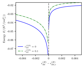
Figure 2: The polaronic energy for $n=2386.2/l_{\perp}$, $a^{(B)}_{s}=0.005l_{\perp}$, $a^{(IB)}_{s}=0.007l_{\perp}$, and $m_{I}=m_{B}$ as a function of $\epsilon^{(B)}_{dd}-\epsilon^{(B)}_{dd,c}$. The blue line is the polaronic energy for the non-dipolar impurity, while the green dash-dotted line is the polaronic energy of an impurity with a finite magnetic moment. The grey dashed line indicates the transition from the superfluid to the supersolid phase.

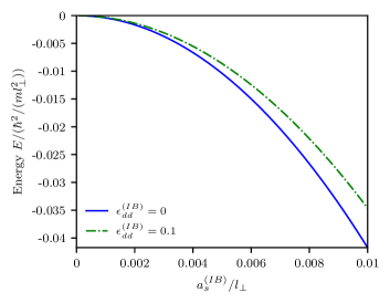
Figure 3: The polaronic energy as a function of the s-wave scattering length $a^{(IB)}_{s}$ in the supersolid regime for $n=2386.2/l_{\perp}$, $a^{(B)}_{s}=0.005l_{\perp}$, $m_{I}=m_{B}$, $\epsilon^{(B)}_{dd}=1.345$, and $\epsilon^{(IB)}_{dd}=0$ (blue line) or $0.1$ (green dash-dotted line).

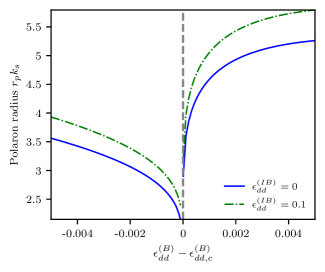
Figure 4: The polaron radius $r_{p}$ in units of $1/k_{s}$ as a function of $\epsilon^{(B)}_{dd}-\epsilon^{(B)}_{dd,c}$ for $n=2386.2/l_{\perp}$, $a^{(B)}_{s}=0.005l_{\perp}$, $a^{(IB)}_{s}=0.007l_{\perp}$, and $m_{I}=m_{B}$. The blue line is the polaronic energy for the non-dipolar impurity, while the green dash-dotted line is the polaronic energy of an impurity with a finite magnetic moment. The grey dashed line indicates the transition from the superfluid to the supersolid phase.

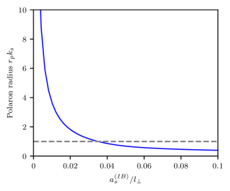
Figure 5: The polaron radius $r_{p}$ in units of $1/k_{s}$ in the supersolid regime as a function of $a^{(IB)}_{s}$ for $n=2386.2/l_{\perp}$, $a^{(B)}_{s}=0.005l_{\perp}$, $m_{I}=m_{B}$, $\epsilon^{(B)}_{dd}=1.345$, and $\epsilon^{(IB)}_{dd}=0$. The grey line indicates the $r_{p}=1/k_{s}$ threshold where the impurity gets localized to a single droplet of the supersolid.

V Conclusion and Outlook

The wavefunction of a one-dimensional dipolar supersolid and the corresponding excitations have been reviewed and discussed. The ground-state energy of an impurity dressed by the excitations of the supersolid has been calculated using the Feynman path-integral method within the Bogoliubov and Fröhlich approximations. A divergence was observed when the supersolid regime was entered. An additional impurity-atom dipole interaction from a finite impurity magnetic moment results in a larger ground-state energy. The polaron radius has also been calculated, showing that for most values, the polaron radius is larger than the size of a single droplet of the supersolid. However, for large enough impurity-atom interaction strengths, the polaron can get localized to a single droplet, behaving like a small polaron. An interesting next step would be to experimentally study the system of an impurity in a dipolar supersolid and compare the results to the path-integral method shown here. Additionally, there are no numerically exact Monte Carlo results for comparison yet for the supersolid polaron system.