Prices and Concentration: A U-shape?
Theory and Evidence from Renewables

Abstract

We study firms’ strategic interactions when each firm may own multiple production technologies, each with its own marginal cost and capacity. Increasing industry concentration by reallocating non-efficient capacity to the largest and most efficient firm can decrease market prices as it incentivizes the firm to outcompete its rivals. However, with large reallocations, the standard monotonic relationship between concentration and prices re-emerges as competition weakens due to the rival’s lower capacity. Thus, we demonstrate a U-shaped relationship between market prices and industry concentration when firms are diversified. This result does not rely on economies of scale or scope. We find consistent evidence from the Colombian wholesale energy market, where strategic firms are diversified with fossil-fuel and renewable technologies, exploiting exogenous variation in renewable capacities. Our findings not only apply to the green transition but also to other industries and suggest new insights for antitrust policies.

JEL classifications: L25, D24, Q21
Keywords: diversified production technologies, energy transition, renewable energy, hydropower, storage, supply function equilibrium, oligopoly

1 Introduction

Economic models typically assume firms use a single technology or production function, resulting in a single marginal cost for any level of production (e.g., Olley and Pakes, 1996). However, firms can often produce the same good using multiple technologies, each with different capacities and marginal costs. These technologies can act as substitutes, replacing each other in production or as complements, providing a firm with the opportunity to influence market prices by simultaneously producing with different technologies. Nonetheless, there is a lack of understanding about how firms make production and pricing decisions with multiple technologies. This gap is crucial for energy firms, where environmental challenges require them to diversify their technology portfolio by including renewables (e.g., Elliott, 2024, Gonzales et al., 2023).

How do firms with multiple production techonologies compete? In this paper, we define a firm as diversified if it can produce the same good using technologies with different marginal costs and capacities. We introduce new theoretical and empirical evidence to study the strategic decisions of such firms. Our analysis is based on the Colombian wholesale energy market, where major suppliers own both renewable (dams) and conventional thermal generators (fossil fuels). Droughts provide exogenous variations in a firm’s renewable capacities without affecting those of conventional generators. Typically, a firm responds to a drought by reducing its hydropower supply, which increases the market price but lowers the firm’s market share. A diversified firm, however, can maintain its market share by increasing production with its conventional generators, as illustrated in Figure 1. This additional supply (gap between red and blue curves) lowers the market price and helps the firm conserve water, as production shifts from hydro to conventional sources. The steeper the firm’s demand curve, the greater its market power, but the more prices will drop as the firm increases its conventional supply. This demonstrates how considerations of market power become non-trivial with diversified firms. Similar incentives may arise in other industries due to mergers (e.g., Morck et al., 1990, Atalay et al., 2019) or trade disruptions altering firms’ boundaries (e.g., Acemoglu and Tahbaz-Salehi, 2024).

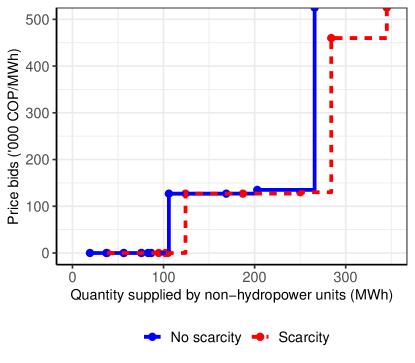
Figure 1: Impact of scarcity on non-affected generators

The figure plots the supply schedule of the non-hydropower generators owned by a Colombian diversified energy firm when it either faces scarcity (red dashed line) or not at its dams. Scarcity is defined as observing a water inflow in the first two deciles of its distribution. The red supply schedule was submitted by ENDG on December 12, 2010 at noon, whereas the blue schedule was submitted two weeks before. Total demand differ by less than 1% in the two markets.

Our main finding is a novel U-shaped relationship between market prices and industry concentration when firms are diversified and face uncertain demand. This U-shaped pattern arises because a firm with a highly efficient technology can disrupt its competitors by producing at their marginal cost, potentially driving them out of the market. When the market leader has limited efficient capacity, we show that reallocating a small amount of inefficient capacity from its competitors to the market leader incentivizes the leader to crowd them out further in low-demand scenarios while relying on the newly added inefficient capacity in high-demand situations. This increase in market concentration can lower market prices as competitors expand their supply to maintain market shares. Conversely, complete crowding out may not always be the optimal strategy, as a firm might prefer raising prices when competition decreases. We demonstrate that large capacity reallocations increase prices as competition weakens due to rivals’ low capacity, resulting in a U-shaped relationship between prices and industry concentration. Quantitatively, our structural model finds that prices drop by up to 10% for small capacity reallocations to the market leader but increase substantially for larger transfers.

Thus, the impact of concentration on prices hinges on two factors: the efficiency of each technology a firm possesses and its overall capacity, which generate Bertrand and Cournot forces, respectively. Market prices generally decrease with small capacity reallocations as firms employ their most efficient technology more but increase with larger reallocations, forming a U-shaped pattern. In contrast, prices will always rise with concentration if the market leader has abundant low-cost capacity, because, in essence, the leader is not diversified, eliminating any crowding-out incentives. The latter result echoes standard trade and industrial organization models (e.g., Atkeson and Burstein, 2008, Nocke and Whinston, 2022), where markups increase with a firm’s market share, justifying the usage of Herfindahl Indices (HHI) as a measure of industry market power. A consequence of our results is that such measures lose meaning when firms are diversified.

More broadly, in oligopolistic industries where the efficient technology is scarce, a larger diversified market leader might result in smaller market prices than if its inefficient technology were allocated to a smaller rival. Our results also extend to studying the price effect of mergers rather than capacity transfers while relaxing the common assumption that the new firm’s marginal cost equals the minimum of the merging parties. Our insights find applications across diverse sectors. For example, in the industrial sectors, firms commonly produce aluminum with various technologies (Collard-Wexler and De Loecker, 2015). In oil and gas, a firm owns reservoirs with different costs and capacities (Asker et al., 2019, Fioretti et al., 2022). In healthcare, hospitals can complement doctors’ advice with cheaper artificial intelligence algorithms (Agarwal et al., 2023).

We theoretically examine the behavior of diversified firms through a static homogeneous-good oligopoly game where firms confront demand uncertainty and own both low- and high-cost technologies, representing hydropower and thermal generation, respectively. Each technology features its own cost curve, which becomes vertical at capacity. A firm’s total cost is the horizontal sum of its technologies’ cost curves, and, hence, it is increasing in the quantity produced. The equilibrium price is determined by firms submitting supply schedules detailing the quantity they are willing to produce at various market prices, following the supply function equilibrium concept proposed by Klemperer and Meyer (1989). This concept, unlike traditional models such as Cournot and Bertrand, is ex-post optimal and encompasses them as extreme cases by permitting any non-negative slope at different market prices.

Initially, in this market, no firm is diversified and the largest firm also has the most efficient technology. We then study what happens when we diversify it by reallocating high-cost capacity to this market-leading firm in different scenarios. If the leader’s low-cost capacity was substantially larger than that of its rivals before the transfer, as under the abundance of hydropower, we find that the transfer reduces its rivals’ ability to compete, leading to higher prices. Therefore, when the leader’s market power comes from its total size, reallocating capacity to the leader effectively “removes resources from the market,” as the leader prioritizes its low-cost technology in production over the high-cost one to minimize costs, following the so-called merit order.

Conversely, the same reallocation of high-cost capacity “brings capacity back into the market” when the leader’s relative capacity advantage is not as large even though being the largest firm. Because of the merit order, the new capacity will be produced only after the exhaustion of its low-cost one, hence only in high-demand situations. However, the firm cannot expand its supply only from a high price onward because this strategy encourages undercutting by its rivals. Hence, both the market leader and its competitors expand their supply schedules, resulting in lower prices than before the reallocation despite more capacity concentration. Importantly, standard synergies like economies of scale play no role in this economy because average costs stay unchanged at the realized market price. Therefore, our results illustrate two sources of market power when firms are diversified: total capacity, driving prices up, and relative efficiency, driving them down.

Alternatively, if a significantly large portion of the high-cost capacity is transferred to the market leader – imagine the extreme scenario where it becomes a monopolist – we demonstrate that market prices invariably increase. This is because the firm can now reduce its production to raise prices without losing inframarginal units, explaining the U-shaped relationship between prices and concentration.

Our empirical investigation centers on the Colombian energy market for several reasons. Firstly, all major players in this market operate diversified production, utilizing a mix of hydropower and thermal energy. Secondly, regulatory requirements ensure the availability of data on firms’ desired production for each technology they employ, a rarity in many other industries. Thirdly, natural fluctuations in weather patterns provide an exogenous factor affecting hydropower capacity, allowing us to study market power and concentration without relying on potentially endogenous events like mergers.

To quantify the impact of diversification on market prices, we extend the theoretical model to account for the main features of the Colombian energy market. In particular, thermal capacity is consistently available, while dry and abundant spells directly influence a firm’s hydropower capacity by altering the opportunity cost of its supply. Empirically, we exploit variation in this opportunity cost as a shifter to a firm’s hydropower capacity, as it does not affect its operating cost and the costs and capacities of other technologies.

To causally identify this U-shape in the data, we simulate market prices in different scenarios where we exogenously endow the market-leading firm with increasing fractions of its competitors’ thermal capacity. The model primitives – the marginal cost of thermal and hydropower generators and the intertemporal opportunity cost of holding water – are identified from the first-order conditions. We estimate the model on hourly markets between 2010 and 2015 and show that the model fits the data well.

Our findings reveal that during droughts, average market prices decline by up to 10% if we double the size of the market leader’s thermal capacity. However, for larger reallocations, prices increase substantially, aligning with the conclusions from models featuring non-diversified firms. During abundant periods, reallocations diminish rivals’ competitiveness, resulting in higher market prices. Notably, the disparity in prices between dry and abundant spells can be significant, with prices during droughts reaching up to ten times higher. This underscores the welfare benefit of diversification, particularly evident in situations where the low-cost technology is scarce.

Earlier investigations have warned against joining renewable and thermal generators because when firms compete à la Cournot, they benefit by reducing their thermal supplies when they also have renewables, as renewables induce a more inelastic demand (Bushnell, 2003, Acemoglu et al., 2017). In contrast, concurrent work by Fabra and Llobet (2023) shows that diversifying suppliers competing à la Bertrand can lead to lower prices if a firm has private information about its realized renewable capacity, as is common for solar and wind farms. However, in our case, we observe different behavior: firms increase rather than decrease thermal generation when facing scarcity.

We provide a unifying account featuring results from both types of conduct that allows us to discuss when diversifying production increases or decreases market prices. Instead of asymmetric information, as Colombian suppliers are aware of each others’ water stocks, we explain the thermal generators’ strategies through their market power, which pushes them to steal market shares when they internalize higher prices due to scarcity. As the storability of solar and wind resources continues to improve (Schmalensee, 2019, Koohi-Fayegh and Rosen, 2020, Andrés-Cerezo and Fabra, 2023), we expect our results to apply also to other renewables, in which case firms could substitute across renewables technologies, without the need for polluting thermal generators, thereby speeding the transition by solving renewables’ intermittency problems (Gowrisankaran et al., 2016, Vehviläinen, 2021) and making it more affordable (Butters et al., 2021).

How might our findings guide policy decisions? Antitrust regulation emerges as an innovative tool for driving down the costs of the green transition, complementing standard approaches like subsidies (Acemoglu et al., 2012, Abrell et al., 2019, Ambec and Crampes, 2019). While existing literature examines subsidy regulations for renewable capacities and grid integration to foster competition and maintain low energy prices (e.g., De Frutos and Fabra, 2011, Ryan, 2021, Elliott, 2024, Gowrisankaran et al., 2022, Gonzales et al., 2023), it often overlooks how ownership of new and old technologies affects pricing. Our findings open new questions regarding firms’ efficient ownership structures. For example, Colombia limits firms to holding no more than 25% of the total installed capacity to prevent market power abuses. However, this threshold also hampers the advantages of diversified production. Although determining the ideal threshold exceeds the scope of this paper, we contend that it should vary according to a firm’s technological capabilities.

Despite an extensive literature questioning the treatment of capital as a homogeneous input (e.g., Robinson, 1953, Solow, 1955, Sraffa, 1960), previous studies have primarily focused on competition among multiproduct firms (e.g., Nocke and Schutz, 2018b) or capacity constraints in firms operating with a single production technology (Kreps and Scheinkman, 1983, Bresnahan and Suslow, 1989, Staiger and Wolak, 1992, Froeb et al., 2003). This paper explores how diversification generates strategic complementarities within firms and across competitors. Our findings highlight two key implications. First, conventional production function estimation methods may fail to capture productivity gains from factor-augmenting technologies (e.g., Demirer, 2022) without specific technology-level data. Second, our results inform antitrust policies regarding divestitures required of merging entities (Compte et al., 2002, Friberg and Romahn, 2015), suggesting that divestitures could inadvertently raise prices by reducing technology diversification.

The paper is structured as follows: Sections 2 and 3 introduce the Colombian wholesale market, describe the data, and present empirical patterns of supply decisions during scarcity and abundance periods. Section 4 explains these patterns through a simple theoretical framework, which forms the basis of our empirical analysis developed in Sections 5 and 6. Finally, Section 7 concludes by discussing our contributions to antitrust policies and the green transition.

2 The Colombian Wholesale Energy Market

This section provides an overview of the Colombian energy market, focusing on the available technologies and its institutions.

2.1 Generation

Colombia boasts a daily energy production of approximately 170 GWh. Between 2011 and 2015, the market featured around 190 generators owned by 50 firms. However, it exhibits significant concentration, with six major firms possessing over 50% of all generators and approximately 75% of total generation capacities. The majority of firms operate a single generator with limited production capacity.

These major players diversify their portfolios, engaging in dam and other generation types, including thermal sources such as fossil fuel-based generators (coal and gas). Additional sources comprise renewables like wind farms and run-of-river, which utilizes turbines on rivers without water storage capabilities. Figure 2a illustrates the hourly production capacities (MW) for each technology from 2008 to 2016, revealing that hydropower (blue) and thermal capacity (black) constitute 60% and 30% of the industry’s capacity, respectively. Run-of-river (green) accounts for less than 6%. Solar, wind, and cogeneration technologies producing energy from other industrial processes are marginal.

Despite the presence of various sources, hydropower dominates production, averaging around 75% of total dispatched units. The remaining energy needs are met by thermal generation (approximately 20% of total production) and run-of-river (5%). However, production varies over time, as shown in Panel (b) of the same figure, which contrasts production across technologies with dry seasons represented by periods of high temperature or low rainfall at dams (gray bars). During dry spells, hydropower production decreases, and thermal generation compensates for water scarcity. Firms strategically stockpile fossil fuels like coal and gas ahead of anticipated dry spells (Joskow, 2011), with their prices closely tied to global commodity markets. In contrast, run-of-river energy lacks storage capabilities, limiting its ability to offset hydropower shortages.

Thermal generation typically incurs higher marginal costs than hydropower. Figure 3 highlights that wholesale energy prices more than double during scarcity periods. Prices experienced a further increase during the sustained dry spell caused by El Niño in 2016 and the annual dry seasons (December to March).

Figure 2: Installed capacity and production volumes by technology over time

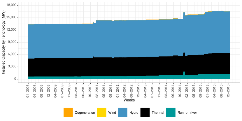
(a) Total installed capacity by technology

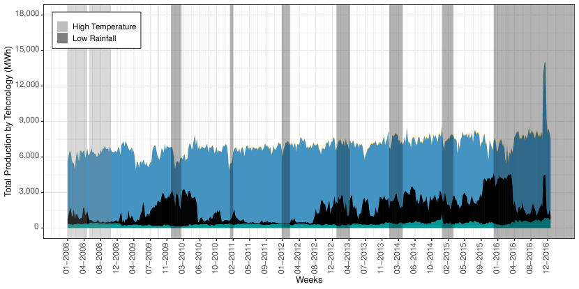
(b) Total weekly production by technology

Note: The figure illustrates the total installed capacity (top panel) and production volumes (bottom) by technology. The vertical bars in Panel (b) refer to periods where a hydropower generator experiences a temperature (rainfall) that is at least one standard deviation above (below) its long-run average.

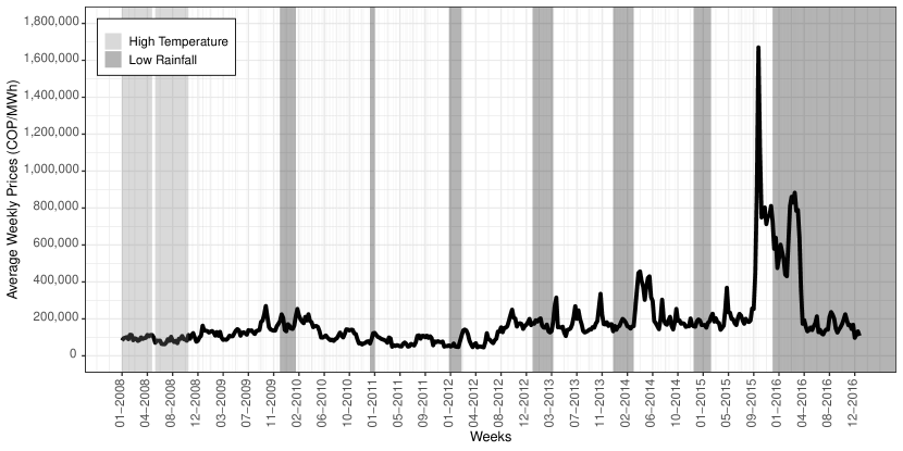
Figure 3: Market prices

Note: Average market prices across weeks. The vertical gray columns refer to periods where a hydropower generator experiences a temperature (rainfall) that is at least one standard deviation above (below) its long-run average. 2,900 COP $\simeq$ 1 US$.

2.2 Institutional Background

The Colombian wholesale energy market is an oligopolistic market with high barriers to entry, as suggested by the fact that the total hourly capacity in Panel (a) of Figure 2 is almost constant over time, and especially so in the period 2010-2015, on which we focus in the following analysis. In this period, only nine generators entered the market (out of 190), all belonging to different fringe firms, leading to a mild increase in market capacity (+4%). The market is highly regulated and consists of a spot and a forward market.

The spot market. The spot market, also known as day-ahead market, sets the output of each generator. It takes the form of a multi-unit uniform-price auction in which Colombian energy producers compete by submitting bids to produce energy the following day. Through this bidding process, each generator submits one quantity bid per hour and one price bid per day. Quantity bids state the maximum amount (MWh) a generator is willing to produce in a given hour, while price bids indicate the lowest price (COP/MW) acceptable for production. Each generator bids its own supply schedule, potentially considering the payoffs to the other generators owned by the same firm, which we call siblings of the focal generator.

Spot market-clearing. Before bidding, the market operator (XM) provides all generators with estimated market demand for each hour of the following day. After bidding, XM ranks bid schedules from least to most expensive to identify the lowest price satisfying demand for each hour. XM communicates the auction outcomes or despacho economico to all generators. During the production day, actual generation may differ due to production constraints or transmission failures. The spot hourly price is set at the value of the price bid of the marginal generator, with all dispatched units paid the same price.

Forward market. The forward market comprises bilateral contracts between pairs of agents. These contracts allow agents to decide the financial position of each generator weeks in advance, serving to hedge against uncertainty in spot market prices. In our dataset, we observe each generator’s overall contract position for each hourly market.

2.3 Data

The data come from XM for the period 2006–2017. We observe all quantity and price bids and forward contract positions. The data also includes the ownership, geolocalization, and capacity for each generator, and daily water inflows and stocks for dams. We complement this dataset with weather information drawn from the Colombian Institute of Hydrology, Meteorology, and Environmental Studies (IDEAM). This information contains daily measures of rainfall and temperature from 303 measurement stations.

Rainfall forecasts are constructed using monthly summaries of el Niño, la Niña, and the Southern Oscillation (ENSO), based on the NINO3.4 index from the International Research Institute (IRI) of Columbia University. ENSO forecasts, published on the 19th of each month, provide probability forecasts for the following nine months, aiding dams in predicting inflows. We have monthly information from 2004 to 2017.

This dataset is complemented with daily prices of oil, gas, coal, liquid fuels, and ethanol – commodities integral to energy production through thermal or cogeneration (e.g., sugar manufacturing) generators.

3 Diversified Production: Empirical Evidence

This section leverages exogenous variations in water inflow forecasts, impacting the capacities of dams, to offer novel perspectives on the production decisions made by diversified firms. Sections 3.1 and 3.2 delineate the empirical methodology and present the primary findings. Finally, Section 3.3 examines the ramifications for market clearing prices.

3.1 Empirical Strategy

This section outlines the empirical strategy used to assess the responses of a firm’s hydro and thermal supplies to variations in its hydropower capacity, utilizing data from periods of drought and abundance within firms.

We construct inflow forecasts for each hydropower generator employing a flexible autoregressive distributed-lag (ARDL) model (Pesaran and Shin, 1995). In essence, these forecasts are derived through OLS regressions of a generator’s weekly average net water inflow, encompassing evaporation, on the water inflows in past weeks and past temperatures, rainfalls, and el Niño probability forecasts. A two-year moving window is used to generate monthly forecasts up to 5 months ahead for the period between 2010 and 2015, where we observe little entry of new plans and no new dams. The forecasting technique is discussed in detail in Appendix B, which also presents goodness of fit statistics.

We investigate generators’ reactions to forthcoming inflows by analyzing the equation:

$$y_{ij,th} =\sum^{L}_{l=1}\left(\beta_{l}^{low}\text{adverse}_{ij,t+l}+\beta_{l}^{high}\,\text{favorable}_{ij,t+l}\right)$$ (1)

$$+\,\textbf{x}_{ij,t-1}\alpha+\mu_{j,m(t)}+\tau_{t}+\tau_{h}+\epsilon_{ij,th}.$$

This equation explores how generator $j$ of firm $i$ updates its current supply schedule $y_{ij,th}$ based on anticipations of favorable ($\text{favorable}_{ij,t+l}$) or adverse ($\text{adverse}_{ij,t+l}$) forecasts $l$ months ahead relative to its average forecast. To minimize autocorrelation, we aggregate bids over weeks ($t$) per hour ($h$). Instances where a generator’s quantity bid falls below the 5^th percentile of the distribution of quantity bids placed by generators of the same technology are excluded to mitigate contamination from unobserved maintenance periods within a week. Importantly, this truncation does not qualitatively impact the results.

The definition of the variables $\{\text{adverse}_{ij,t+l}\}_{l}$ and $\{\text{favorable}_{ij,t+l}\}_{l}$ varies across analysis. Specifically, when focusing on the supply of hydropower, these variables take the value one if dam $j$ of firm $i$ anticipates its $l$-month ahead forecast to deviate by either a standard deviation higher or lower than its long-run average (for the period 2008-2016), and zero otherwise, respectively. Conversely, when transitioning the analysis to sibling thermal generators – those owned by a firm with dams – these indicators are based on the cumulative $l$-month ahead inflow forecasts associated with the dams owned by $i$.

We control for changes in market conditions in $\textbf{x}_{ij,t-1,h}$ utilizing average market demand, water stocks, and forward contract positions (in log) for week $t-1$ and hour $h$. To account for seasonal variations that may impact generators differently, fixed effects are included at the generator-by-month and firm-by-year levels ($\mu_{j,m(t)}$). Macro unobservables, such as variations in demand, are captured through fixed effects at the week-by-year ($\tau_{t}$) and hour levels ($\tau_{h}$). The standard errors are clustered by generator, month, and year.

Exclusion restriction. Identification in (1) relies on the credible assumption that a firm’s current bidding does not directly depend on past temperatures and rains at the dams but only indirectly through water inflows. This restriction is credible because a generator should only care for its water availability rather than the weather per se – due to their rural locations, the local weather at the dam is unlikely to influence other variables of interest to a generator, like energy demand in Colombia, which is controlled for in the estimation. Appendix C is dedicated to robustness checks and also proposes an alternative estimation strategy where generators respond symmetrically to favorable and adverse forecasts. The Appendix also discusses the information content of our inflow forecasts by showing that generators’ responses to forecast errors – the observed inflow minus the forecasted inflow – are insignificant.

3.2 Results

3.2.1 Hydropower Generators

Figure 4 displays the coefficients, $\{\beta^{low}_{l}$,$\beta^{high}_{l}\}_{l}$, from (1). The dependent variable is the logarithm of hydropower generator $j$’s price bid in Panel (a) and quantity bid in Panel (b). Coefficient magnitudes represent percentage changes when facing an adverse forecast (red circles) or a favorable forecast (blue triangles) one, three, or five months ahead.

Dams strategically adjust their supply schedules in anticipation of extreme events. They adapt their supplies mainly by changing their quantity bids rather than their price bids because, having low marginal costs, they always produce and the market asks for hourly quantity bids but only daily price bids. We find that dams decrease their supply schedules ahead of adverse events, recognizing the negative impact of capacity constraints (e.g., Balat et al., 2015), and increase them ahead of favorable forecasts. Notably, generators are more responsive to adverse events: generation decreases by 7.1% for one-month adverse forecasts and 1.3% for two-month adverse forecasts, whereas it only increases by approximately 3.7% one month ahead of a favorable forecast.

3.2.2 “Sibling” Thermal Generators

Figure 5 presents the estimation results of (1) on thermal generators that are sibling to dams. Due to the absence of water stocks for thermal generators, we include a control for a firm’s lagged total water stock in $\textbf{x}_{ij,t-1}$. The results unveil distinct responses of sibling thermal generators to forecast inflows compared to hydropower generators. Sibling thermal generators increase their supply schedule before favorable events (blue triangles) and decrease it before adverse ones (red circles). They primarily adjust through their price bids because, given their high marginal costs, they are not operational at all times and lack the flexibly to vary production across hourly markets. Finally, although the analysis indicates that they respond to extreme events well before hydropower generators, it is worth noting that this analysis focuses on extreme firm-level forecasts rather than generator-level forecasts as in the previous section, which might be less severe.

Figure 4: Hydropower generators’ responses to inflow forecasts

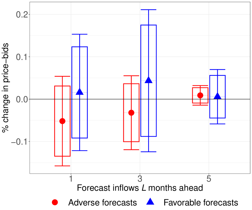
(a) Price bids

(b) Quantity bids

Notes: The figure studies how hydropower generators respond to favorable or adverse future water forecasts according to (1). Each plot reports estimates of $\{\beta^{low}_{l}\}$ in red and $\{\beta^{high}_{l}\}$ in blue for one, three, and five months ahead. Error bars (boxes) report the 95% (90%) CI.

Figure 5: Thermal generators responses to sibling hydro generators’ inflow forecasts

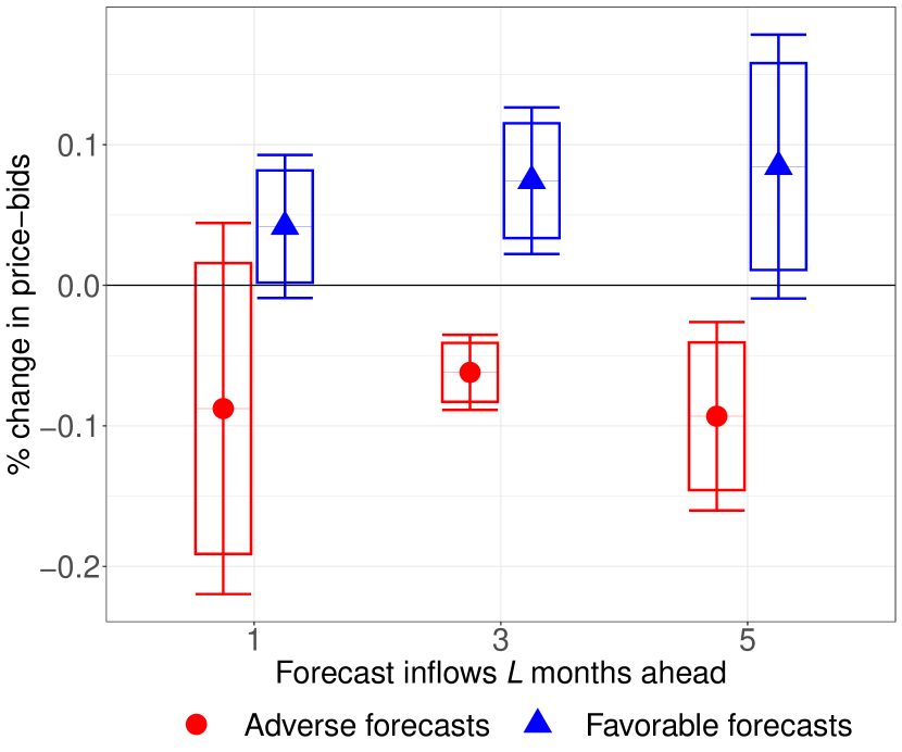
(a) Price bids

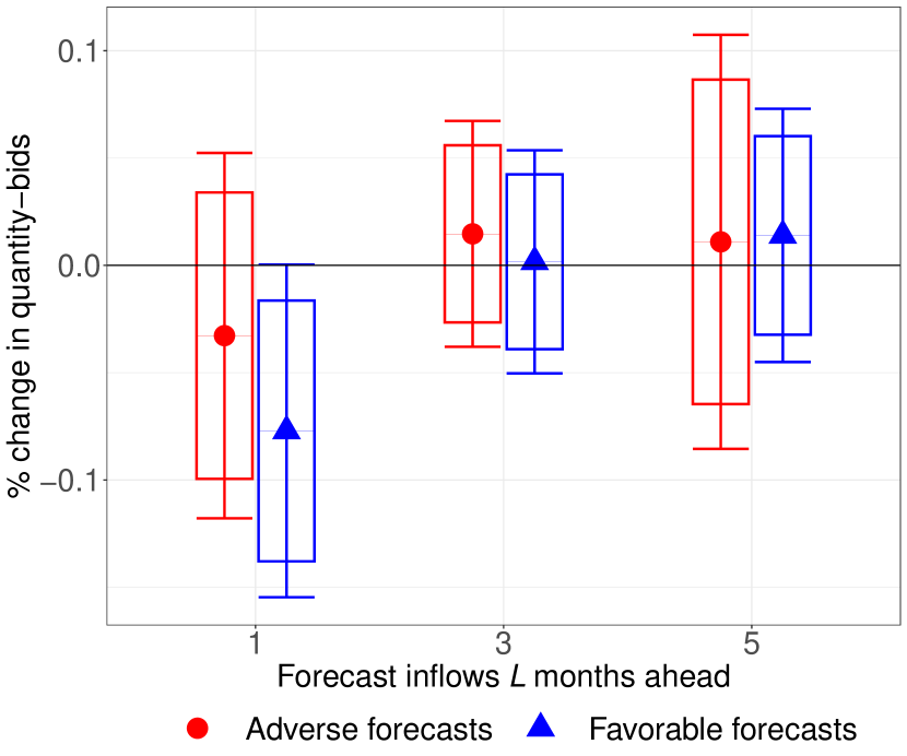
(b) Quantity bids

Notes: The figure studies how sibling thermal generators respond to favorable or adverse future water forecasts according to (1). Each plot reports estimates of $\{\beta^{low}_{l}\}$ in red and $\{\beta^{high}_{l}\}$ in blue for one, three, and five months ahead. Error bars (boxes) report the 95% (90%) CI.

3.2.3 Competitors’ Inflow Forecasts

To comprehensively understand firms’ responses to future shocks, we explore whether hydropower generators incorporate reactions to competitors’ forecasts. We model adverse and favorable inflows in (1) based on the sum of inflows at a firm’s competitors. We allow for distinct slopes for each generator’s water stock to control adequately for current water availability at various dams in $\textbf{x}_{ij,t-1}$. Figure 6 reveals minimal movement in a firm’s bid concerning its competitors’ forecasts, with magnitude changes generally within $\pm 1\%$ and lacking statistical significance. Separate joint significance tests for adverse and favorable forecasts do not reject the null hypothesis that they are zero at standard levels.

Figure 6: Responses to competitors’ inflow forecasts

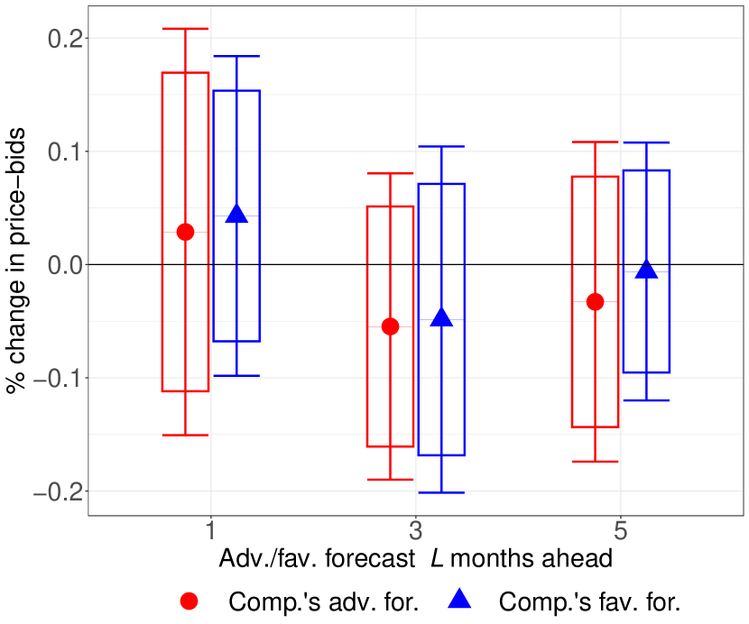
(a) Price bids

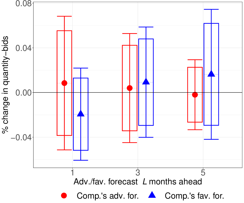
(b) Quantity bids

Notes: The figure studies how generators respond to favorable or adverse future water forecasts accruing to competitors according to (1). Each plot reports estimates of $\{\beta^{low}_{l}\}$ in red and $\{\beta^{high}_{l}\}$ in blue for one, three, and five months ahead. Error bars (boxes) report the 95% (90%) CI.

Appendix C.1.3 further extends this analysis in two dimensions. First, it demonstrates that generators respond to their own inflow forecasts but not to the inflow forecasts of competitors. Second, despite the potential informativeness of competitors’ water stocks, it offers suggestive evidence against this hypothesis. Consequently, generators do not appear to react substantially to the crucial potential state variables of their competitors. This observation, while potentially counterintuitive in a competitive context, finds parallels in industrial organization literature. For instance, Hortaçsu et al. (2021) show that airline carriers employ simple heuristics in pricing, disregarding the pricing of other airline companies. Similar to hydropower generators, airline firms grapple with forecasting seat demand (inflows) across various routes (dams). In both scenarios, focusing on their own state variable while overlooking those of competitors may simplify a complex problem.

3.3 Implications for Market Prices

Firms strategically deploy their thermal technology differently during periods of abundance (high inflows) and scarcity (low inflow). To assess whether a greater unshocked capacity (i.e., thermal) can alleviate the price hike resulting from dry spells, we capitalize on the exogenous occurrence of such periods across firms with different thermal capacity.

We base our analysis on the following regression model,

$$\ln(p_{th}) =\sum^{L}_{l=1}\Big{[}\gamma_{l}^{low}\sum_{i}\Big{(}\text{adverse}_{i,t+l}\,K^{T}_{it}\Big{)}+\gamma_{l}^{high}\sum_{i}\Big{(}\text{favorable}_{i,t+l}\,K^{T}_{it}\Big{)}\Big{]}$$ (2)

$$+\sum^{L}_{l=1}\Big{[}\beta_{l}^{low}\sum_{i}\text{adverse}_{i,t+l}+\beta_{l}^{high}\,\sum_{i}\text{favorable}_{i,t+l}\Big{]}$$

$$+\gamma^{cap}\sum_{i}K^{T}_{it}+{\textbf{x}}_{t-1,h}\mathbf{\alpha}+\tau_{th}+\epsilon_{t},$$

where the logarithm of the hourly average weekly price is on the left-hand side. On the right-hand side, the first line of (2) features the interaction between whether a firm expects adverse or favorable inflow forecasts $l$-months ahead with its total sibling thermal capacity in GWh, $K^{T}_{it}$. We expect that the greater thermal capacity available to generators with adverse forecasts, the lower the price ($\gamma^{low}_{l}<0$), and vice-versa for favorable inflows ($\gamma^{high}_{l}>0$) if thermal generators do not operate in similar periods (cf. Figure 5). The remaining two lines of (2) control for the direct effect of adverse and favorable forecasts and total thermal capacity on spot prices. Finally, ${\textbf{x}}_{t-1,h}$ includes lagged market outcomes, such as hourly average weekly demand and forward contracts, in logs. As error terms are likely correlated across seasons and hourly markets, we cluster the standard errors at the month and year level.

Table 1: The impact of technology substitution on spot prices

(1) (2) (3) (4) Average weekly price in hour $h$ ($\ln p_{ht}$) Adverse inflows (3 months), $\gamma^{low}_{3}$ 0.166 0.210^∗∗ 0.334^∗∗ (0.284) (0.058) (0.077) Adverse inflows (5 months), $\gamma^{low}_{5}$ 0.413^∗∗ -0.127 -0.241 (0.126) (0.094) (0.117) Thermal cap. available to adv. inflows (3 months), $\beta^{low}_{3}$ -1.303 -1.746^∗∗ -2.769^∗∗ (2.539) (0.540) (0.747) Thermal cap. available to adv. inflows (5 months), $\beta^{low}_{5}$ -3.508^∗∗∗ 0.875 1.979 (0.492) (0.721) (0.944) Favorable inflows (3 months), $\gamma^{high}_{3}$ 0.032 0.021 -0.162^∗∗ (0.203) (0.037) (0.044) Favorable inflows (5 months), $\gamma^{high}_{5}$ 0.374 0.001 -0.368^∗ (0.195) (0.083) (0.154) Thermal cap. available to fav. inflows (3 months), $\beta^{high}_{3}$ -0.038 -0.045 1.380^∗∗ (1.654) (0.249) (0.348) Thermal cap. available to fav. inflows (5 months), $\beta^{high}_{5}$ -2.939 0.064 3.133^∗ (1.722) (0.741) (1.322) Total sibling thermal capacity (GW), $\gamma^{cap}$ -0.012^∗∗ -0.007^∗∗∗ -0.005^∗∗∗ -0.020^∗∗∗ (0.003) (0.001) (0.001) (0.003) Lag demand (ln) $\checkmark$ $\checkmark$ $\checkmark$ Lag contract position (ln) $\checkmark$ $\checkmark$ $\checkmark$ Lag water stock (ln) $\checkmark$ Lag spot price (ln) $\checkmark$ FE: Hour $\checkmark$ $\checkmark$ $\checkmark$ $\checkmark$ FE: Year-by-season $\checkmark$ FE: Year-by-month $\checkmark$ $\checkmark$ $\checkmark$ Subset All All Dry season Wet season $N$ 7,464 7,464 2,424 5,040 R2 Adj. 0.639 0.934 0.920 0.915 * – $p<0.1$; ** – $p<0.05$; ^∗∗∗ – $p<0.01$

• Notes: This table shows the estimated coefficients from (2). The main regressors are the number of adverse (rows 1 and 2) and favorable inflows (rows 5 and 6) and their interactions with the thermal capacity available to the firms that expect an adverse (rows 3 and 4) and a favorable inflow (rows 7 and 8). All variables are standardized. Column 1 includes fixed effects by year-by-season, while the remaining columns have fixed effects by year-by-month. Column 3 examines adverse inflow in dry seasons (from December to March) and Column 4 examines favorable inflows in wet seasons (from April to November). Standard errors clustered by year and month.

Table 1 presents the results, where we focus on forecasts three and five months ahead to avoid the correlation between the current total water stocks and the one- and two-month ahead forecasts. Column (1) controls for current market conditions using lag demand and forward contract position, as well as hydropower availability using total water stock. Fixed effects are at the hour and at the year-by-season (dry or rainy) level. Column (2) utilizes lag spot prices to control for market conditions and month-by-year fixed effects to account for hydropower availability. All regressors, including those that are a function of multiple variables, are standardized.

The estimates in Column (1) indicate that a one standard deviation increase in the number of adverse inflows expected three to five months ahead increases current prices. However, a concurrent one-standard-deviation increase in the sibling thermal capacity available partially compensates for these higher prices. Column (2) produces qualitatively similar findings, with the primary difference being that the largest effect appears three months ahead instead of five. This result can be attributed to the different controls, as including the lagged water stock in Column (1) captures some variation pertaining to three-month forecasts, as it correlates more strongly with the three-month forecasts than the five-month ones.

The results are less clear for favorable inflows, likely stemming from a correlation across forecasts. To gain deeper insights into the impact of favorable inflows on market prices, we refine our analysis by subsetting the sample in Columns (3) and (4). Specifically, we focus on adverse forecasts during dry seasons and favorable forecasts during wet seasons to further highlight the capacity constraint mechanism. The analysis confirms the previous results during droughts (Column 3). However, the opposite holds during wet seasons (Column 4). Here, prices are, on average, lower ahead of favorable inflows as dams expand their supplies. At the same time, thermal generators decrease their own supplies according to the mechanism outlined in Section 3.2.2. Therefore, more thermal capacity at firms expecting abundance increases market prices as these firms “take capacity out of the market” by decreasing their thermal supplies.

These findings hold significant implications for policy. The concentration of thermal capacity around firms expecting droughts may potentially decrease market prices, while conversely, it could raise prices during periods of expected abundance of renewables. To fully understand this result, the following sections introduce an oligopoly model to examine how diversified firms wield their market power under diverse capacity configurations. Then, we extend and estimate the model using data from the Colombian wholesale energy market, conducting counterfactual exercises to quantify the price benefits resulting from moving thermal capacity to renewable suppliers.

4 A Competition Model With Diversified Firms

This section introduces an oligopoly model that reproduces the key empirical findings from the preceding section. Firms exhibit diversified production, enabling each to produce the same homogeneous good by means of technologies with differing marginal costs and capacities. In this context, market dominance hinges on either a firm’s larger overall capacity or the superior efficiency of one of its technologies. When a firm dominates in capacities, it acts as a monopolist on the market unsatisfied by its competitors. Conversely, having the most efficient technology helps a firm “crowd out” its competitors by selling below their marginal cost. We find that the opposing impacts of these two sources of market power on market outcomes produce the empirical patterns in Section 3.2.

The firm’s problem. Consider an oligopolistic market where firms sell a homogeneous good, such as electricity, and face an inelastic market demand, $D(\epsilon)$, subject to an exogenous shock $\epsilon$ shifting demand horizontally, with a strictly positive density in $[\underline{\epsilon},\overline{\epsilon}]$. Before $\epsilon$ is realized, firm $i$ commits to a supply schedule, $S_{i}(p)$, which maximizes

$$\max_{S_{i}(\cdot)}E_{\epsilon}\Big{[}\pi_{i}\Big{]}=E_{\epsilon}\Big{[}p\cdot S_{i}(p)-C_{i}\left(S_{i}(p)\right)\Big{]},\,\,\,\,\text{s.t.}\,\,\,\,S_{i}(p)=D(\epsilon)-\sum_{j\neq i}S_{j}(p),$$ (3)

where $C(\cdot)$ is firm $i$’s cost of producing $S_{i}(p^{*})$ at the market price, $p^{*}$. The market clearing constraint forces firm $i$’s supply to equate its residual demand, $D^{R}_{i}(p^{*},\epsilon)\equiv D(\epsilon)-\sum_{j\neq i}S_{j}(p^{*})$, which is the demand not satisfied by $i$’s competitors at $p^{*}$.

We adopt the supply function equilibrium (SFE) concept proposed in the seminal work of Klemperer and Meyer (1989), in which firm $i$ selects $S_{i}(p)$ by best-responding to the supply of its competitors, $S_{-i}(p)$, to maximize (3). SFEs come with two key advantages. First, we need no assumption on firm’s beliefs about the random demand shock $\epsilon$: Klemperer and Meyer (1989) demonstrate that maximizing (3) with respect to a function, $S_{i}(p)$, is equivalent to choosing the optimal price $p$ for every possible demand realizations $D(\hat{\epsilon})$, or $\max_{p}\pi_{i}(p,\hat{\epsilon})=p\cdot D^{R}_{i}(p,\hat{\epsilon})-C_{i}(D^{R}_{i}(p,\hat{\epsilon}))$. By varying $\hat{\epsilon}$, we obtain all possible realizations of $D^{R}_{i}(p,\hat{\epsilon})$ in which firm $i$ best responds to all its competitors: these quantity-price combinations, $(D^{R}_{i}\big{(}p(\hat{\epsilon}),\hat{\epsilon}\big{)},p(\hat{\epsilon}))$, depict the $S_{i}(p)$ that solves (3).

Second, this ex-post optimality property does not apply to other standard models of competition like Bertrand and Cournot under demand uncertainty and increasing marginal costs. This property makes SFEs a natural equilibrium concept to examine the behavior of a firm whose technologies have different marginal costs and capacities. In addition, by allowing any non-negative supply slope, SFEs include these competition models as limiting cases: a horizontal schedule (a price for all quantities) aligns with Bertrand, while a vertical schedule (a quantity for all prices) aligns with Cournot.

Baseline (non-diversified firms). There are three production technologies: a low-, a high-, and a fringe-cost technology, with constant unit costs $c^{l}$, $c^{h}$, and $c^{f}$, respectively, with $c^{l}<c^{h}<c^{f}$, non-negative, and finite. Firm $i$’s technology portfolio $K_{i}$ is a vector detailing its capacity of low-, high- and fringe-cost technologies, namely, $K_{i}=(K_{i}^{l},K_{i}^{h},K_{i}^{f})$. Hence, $C_{i}=\sum_{\tau}c^{\tau}\cdot S_{i}^{\tau}(p)$ depends on its technology-specific supply, $S_{i}^{\tau}(p)$, at price $p$.

There are $N>1$ firms, with none of the firms being diversified in this baseline scenario. The technology portfolios of the strategic firms are $K_{1}=(K_{1}^{l},0,0)$ for Firm 1 and $K_{2}=(0,K_{2}^{h},0)$ for Firm 2. Firm 1 can be viewed as a supplier of cheap renewable energy, such as a dam, and Firm 2 as a fossil-based generator. Given the size of dams in the empirical application, we assume that $K_{1}^{l}>K_{2}^{h}>0$, making Firm 1 the market leader. The technology portfolio of fringe firm $i\in(3,...,N)$ is $K_{i}=(0,0,K_{i}^{f})$ and includes only the fringe technology: since $K_{i}^{f}$ is small, these firms are price takers.

The equilibrium supply for strategic firm $i\in(1,2)$ depends on the market price. either firm produces for $p<c^{h}$, as Firm 2, whose marginal cost is $c^{h}$, would make a loss in this price range, while Firm 1 can unilaterally inflate $p$ to (an $\varepsilon>0$ below) $c^{h}$ by not producing for any $p\in[c^{l},c^{h})$ as in Bertran competition. For $p\in[c^{h},c^{f})$, firm $i$’s first-order condition (FOC) is:

$$S_{i}(p)=S^{\prime}_{-i}(p)\cdot(p-c^{\tau}_{i}),\hskip 14.22636pt\mathrm{for}\hskip 14.22636pti\in(1,2).$$ (4)

Hence, in this price range, $S_{i}(p)$ depends on the slope of its competitors’ supply, $S^{\prime}_{-i}(p)$, and the unit cost of the marginal technology that firm $i$ uses in production $\tau\in(l,h)$, resulting in different slopes given a different market price and marginal technology. At $p=c^{f}$, firm $i$ exhausts all its capacity to prevent being crowded out by the fringe firms (i.e., $S_{i}(c^{f})=\sum_{j}K_{i}^{j}$). $S_{i}(p)$ are continuous for any $p$ as a discontinuous supply provides opponents with a profitable deviation by increasing production at a slightly lower price.

Before presenting a formal proposition, we numerically illustrate the equilibrium outcomes in this market in the left panels of Figure 4 and use them to visually compare the impact of diversification, which we illustrate in the right panels. The red (blue) dotted lines report the assumed cost structures of Firm 1 (Firm 2). Under abundance (Panel a), Firm 1’s low-cost capacity is $K_{1}^{l}=9$ but only $K_{1}^{l}=5$ under scarcity (Panel c). The other primitives are constant across scenarios at $c^{l}=0$, $c^{h}=1$, $c^{f}=2$, and $K_{2}^{h}=4$. Solid lines report equilibrium outcomes from the point of view of Firm 1. The solid red line is Firm 1’s supply, $S_{1}(p)$, and its residual demand, $D^{R}_{1}(p)$, is in black. Without loss of generality, we fix the realized market demand at 6 (vertical gray line).

The shape of $S_{1}$ follows (4) and, hence, is quite similar across panels. As mentioned above, $S_{1}(p)=0$ for $p<c^{h}$. At the price level $p=c^{h}$, Firm 1 undercuts its opponent thanks to the greater efficiency of its low-cost technology, similar to the equilibrium that we would observe under Bertrand competition with asymmetric firms. Unlike Bertrand, Firm 1 does not employ all its capacity at this price because firms have incentives to reduce their production, similar to a Cournot game. For every $p\in[c^{h},c^{f})$, the FOC in (4) entails comparing the profits from pricing the marginal unit at $p$ against the alternative case of selling at $p^{\prime}>p$, thereby losing the marginal unit to competitors while raising higher revenues from the inframarginal ones. Hence, the slope of $S_{1}$ becomes positive at large enough quantities and similarly for Firm 2. This tradeoff disappears at $p=c^{f}$, the price at which fringe firms flood the market, so that $S_{i}(c^{f})$ becomes vertical at capacity.

$S_{2}$ has a similar shape to $S_{1}$. $S_{2}$ can be found as the horizontal difference between the gray ($D$) and the black ($D^{R}$) lines, with part of $D^{R}$’s horizontal segment at $p=c^{f}$ shared with the fringe firms, as Firm 2 can price its last units slightly below $c^{f}$ to avoid being crowded out. To avoid cluttering Figure 4, we plot $S_{2}$ in Appendix Figure A1.

Since, in equilibrium, at least one of the two firms must exhaust all its capacity, a key difference arises across the two panels. In Panel (a), Firm 2 exhausts all its capacity as $p\to c^{f}$, while $S_{1}(c^{f})$ is horizontal meaning that Firm 1 is willing to sell multiple units at $p=c^{f}$. This outcome is reversed under scarcity in Panel (c). Here, Firm 2 has a greater ability to unilaterally raise prices for greater demand realizations since Firm 1’s capacity is smaller. As both firms supply less compared to Panel (a), Firm 1 exactly exhausts its capacity as $p\to c^{f}$, while Firm 2 has idle capacity at this price. Scarcity does not prevent Firm 1 from crowding out Firm 2 for low-demand realizations; however, the horizontal segment of $S_{1}$ is now shorter compared to that in Panel (a) as Firm 1 rumps up production earlier to exhaust capacity at $p\to c^{f}$. Equilibrium prices are higher in Panel (c) than in Panel (a), echoing the results in Table 1, which shows that adverse inflows and lower capacities are associated with higher prices.

Figure 7: Equilibrium before and after diversifying Firm 1

(a) Top panel: Abundance of low-cost technology

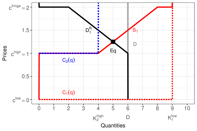
(b) Before the transfer
$K_{1}=(9,0,0)$ & $K_{2}=(0,4,0)$

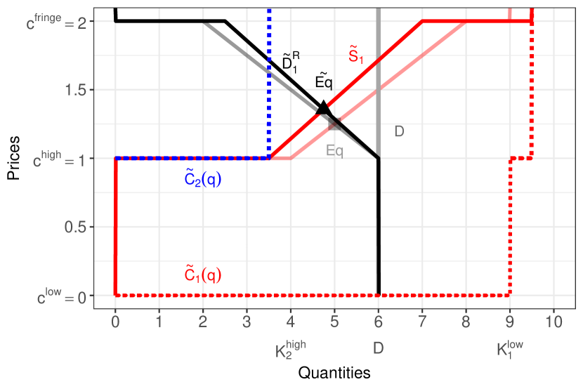
(c) After the transfer
$\tilde{K}_{1}=(9,0.5,0)$ & $\tilde{K}_{2}=(0,3.5,0)$

(d) Bottom panel: Scarcity of low-cost technology

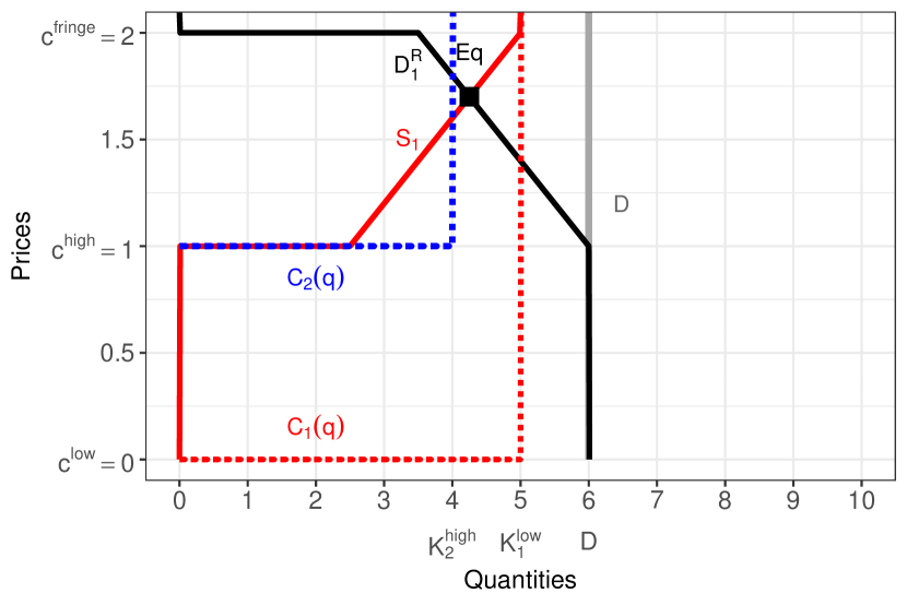
(e) Before the transfer
$K_{1}=(5,0,0)$ & $K_{2}=(0,4,0)$

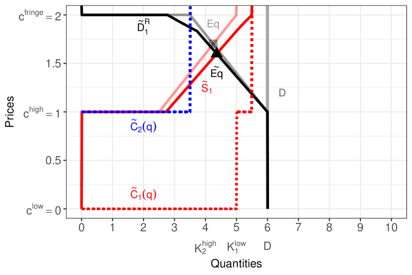
(f) After the transfer
$\tilde{K}_{1}=(5,0.5,0)$ & $\tilde{K}_{2}=(0,3.5,0)$

Notes: Each panel illustrates equilibrium outcomes from the perspective of Firm 1. Solid lines represent equilibrium outcomes, while dotted lines depict marginal cost curves for Firm 1 (red) and Firm 2 (blue). In each panel, the left plot shows outcomes before a capacity transfer, and the right plot shows outcomes after transferring 0.5 units of high-cost capacity from Firm 2 to Firm 1. The shaded square ($Eq$) and curves in the right plot represent the pre-transfer equilibrium, and symbols with a $\sim$ denote post-transfer equilibrium variables. Each subcaption details the technology profile of each firm as $K_{i}=(K_{i}^{l},K_{i}^{h},K_{i}^{f})$. Market demand is constant at 6 (gray solid line), and the cost parameters are $c^{l}=0$, $c^{h}=1$, and $c^{f}=2$.

Equilibrium with diversified firms. To replicate the analysis in Table 1, where we studied market price changes when the firm experiencing a drought (low $K_{1}^{l}$) or abundance (high $K_{1}^{l}$) had more or less thermal capacity ($K_{1}^{h}=0$ or $K_{1}^{h}=\delta>0$), we diversify Firm 1 by considering a reallocation of $\delta=0.5$ units of high-cost technology from Firm 2 to Firm 1. As a result, the technology portfolios in Panels (b) and (d) of Figure 4 change to $\tilde{K}_{1}=(K_{1}^{l},\delta,0)$ and $\tilde{K}_{2}=(0,K_{2}^{h}-\delta,0)$, where we overlaid and shaded the original $S_{1}$ and $D^{R}_{1}$ to compare the market outcome with the relevant baseline scenario.

We find that diversifying Firm 1 has opposite effects on market prices in the two scenarios. First, notice that the new marginal cost curves, $\tilde{C}_{1}$ and $\tilde{C}_{2}$, denote a greater capacity concentration around Firm 1 in Panels (b) and (d) compared to Panels (a) and (c), respectively. Panel (b) presents the standard effects of concentration in oligopolistic markets: as Firm 1 prioritizes its low-cost capacity to its new high-cost one – the so-called, merit order – it employs its high-cost capacity only at $p=c^{f}$. Before the transfer, this capacity was sold by Firm 2 for $p<c^{f}$. Both firms react by decreasing their supply schedules, leading to higher prices, consistent with the role of greater thermal concentration during wet periods, as in Column 4 of Table 1.

In contrast, a similar technology transfer decreases prices under scarcity. In Panel (d), Firm 1 has more capacity than in Panel (c), but it still exhausts its overall capacity ($K^{l}_{1}+\delta$) at $p=c^{f}$ in equilibrium because $\delta$ is small relative to the size of Firm 2 – note that its supply was flat for 1.5 units at $p=c^{f}$ in Panel (c), which effectively are not produced in that equilibrium (Appendix Figure A1). In Panel (d), the transfer enables the firm to employ more of its low-cost technology to outcompete its rivals more than in Panel (c), even though its low-cost capacity $K_{1}^{l}$ stays unchanged, because it alters Firm 1’s trade-off between marginal and inframarginal units at all $p\in[c^{h},c^{f})$, with the new $\delta$ high-cost units utilized for $p$ approaching $c^{f}$. Therefore, after the transfer, Firm 1’s hydropower supply is still steeper under scarcity than under abundance (Panel b), but it expands in Panel (d) compared to Panel (c). On the other hand, comparing Panels (b) and (d), Firm 1’s high-cost capacity is priced at a higher price under abundance than scarcity, which matches the empirical evidence from Panel (a) of Figure 5.

Turning to Firm 2’s best response, the gap between $\tilde{D}^{R}_{1}$ and the shaded pre-transfer $D^{R}_{1}$ whitness Firm 2’s new agressive pricing strategy, as its supply expands for all $p\in[c^{h},c^{f})$ to limit its revenue loss due to Firm 1’s more aggressive pricing. This response is easily detected for prices above the price at which Firm 1 exhausts its $K_{1}^{l}$ units ($p>1.6$). As Firm 2 priced the transferred $\delta$ units exactly at $c^{f}$ before the transfer, but Firm 1 sells them for $p\leq c^{f}$ after it, equilibrium prices decrease compared to Panel (c). This result mirrors the finding in Table 1 that increased thermal capacity among firms anticipating droughts helps temper price surges. It is worth noting that across all panels, Firm 1 exclusively utilizes its low-cost technology at the equilibrium $p$, highlighting the absence of economies of scale because the average cost stays unchanged.

The following proposition generalizes these numerical examples.

Proposition 1

A marginal capacity transfer from Firm 2 to Firm 1 increases the equilibrium price if $K_{1}^{l}>\frac{c^{f}-c^{l}}{c^{f}-c^{h}}K_{2}^{h}$ (abundance scenario) and decreases it if $K_{1}^{l}<\frac{c^{f}-c^{l}}{c^{f}-c^{h}}K_{2}^{h}$ (scarcity scenario).

Proof. See Appendices A.1.1 – A.2.3. $\Box$

The proposition demonstrates that the lower (higher) prices observed when the firm experiencing relative scarcity (abundance) has more high-cost thermal capacity, as depicted in Table 1, are attributable to strategic competition. In addition, the proposition clarifies the exact meaning of scarcity and abundance, as Firm 1’s relative capacity compared to Firm 2, taking into account its cost advantage through the ratio $\frac{c^{f}-c^{l}}{c^{f}-c^{h}}$. In Appendix A.1.1, we show that this equilibrium exists and is unique.

Therefore, diversification can incentivize a more efficient usage of the low-cost technology. If firms had the same technologies, moving capacity from a small to a large firm would always result in higher prices, as it severs Bertrand forces, making one’s capacity the sole source of market power. Similarly, if both Firms 1 and 2 were diversified with the same capacity profile $(K^{l},K^{h},0)$ with $K^{l}>0$ and $K^{h}>0$, moving high-cost capacity from Firm 2 to 1 raises market prices as Firm 2 becomes less competitive at high prices due to Firm 1’s larger high-cost capacity (the proof is in Appendix A.1.3).

Concentration & market power. Our analysis underscores a novel U-shaped relationship between concentration and market prices when efficiency dominates. To see it, focus on the scarcity scenario and imagine that all the capacity of Firm 2 is transferred to Firm 1 instead of just $\delta=0.5$ units, making $S_{2}(p)=0\,\forall p$. Due to such a dominant capacity position, Firm 1 will best respond by selling all its capacity at $c^{f}$, meaning a higher equilibrium price than in Panel (d).

Therefore, if firms are diversified, a small $\delta$-reallocation to the most efficient firm pushes the price down as the receiving firm expands its supply to crowd out its competitors – i.e., Bertrand forces. Further increases in $\delta$ lead to smaller marginal drops in prices, as the greater capacity provides the firm with the standard monopolistic incentives to exclude consumers by raising prices – i.e., Cournot forces. Prices will first drop, reach a plateau, and then increase as shares of capacities are transferred. When capacity dominates instead, any capacity transfers of less efficient technologies to the dominant firm can only raise prices due to the merit order.

General framework. Extending the game presented in the previous section to $N$ strategic players and a downward-sloping market demand, Appendix A.1 finds that when the market clears and uncertainty resolves,

$$\underbrace{\frac{p-c_{i}(S_{i}(p))}{p}}_{\text{Markup}}=\underbrace{\frac{s_{i}}{\eta}}_{\begin{subarray}{c}i\text{'s share of}\\ \text{price elasticity}\end{subarray}}\,\times\,\,\,\,\,\underbrace{\left(1-\frac{S^{\prime}_{i}(p)}{{D^{R}_{i}}^{\prime}(p)}\right)}_{\begin{subarray}{c}\textit{Crowd out ratio }\\ (\geq 1)\end{subarray}}.$$ (5)

As in Cournot, the left-hand side portrays firm $i$’s markup. Unlike Cournot, the right-hand side features not only the price elasticity of demand faced by firm $i$ but also the ratio of the slopes of firm $i$’s supply and residual demand at price $p$, which we term “crowd out.” The ratio in parenthesis is non-negative: if greater than one, $i$ gains market shares from its rivals and loses to them when smaller than one, as $p$ changes marginally. The equilibrium supply balances a firm’s efficiency, as measured by the merit order of $i$’s production technologies, $c_{i}(S_{i}(p))$, with a firm’s capacity dominance, which relates the firm’s technology portfolio to that of its competitors through $S^{\prime}_{i}(p)$ and ${D^{R}_{i}}^{\prime}(p)$.

To gain intuition, imagine either plot in Figure 4 as a grid where prices and quantities are discretized: if at a given price increase $p+h$ competitors increase their supply more than $i$, then $i$ loses quotes of the market as $S_{i}(p+h)-S_{i}(p)<D^{R}_{i}(p)-D^{R}_{i}(p+h)$. In standard oligopoly games, firms only internalize that increasing production decreases prices through the price elasticity, (${s_{i}}/{\eta}$), but do not internalize the strategic response of their competitors through the slope of their supplies (${D^{R}_{i}}^{\prime}(p)=D^{\prime}(p)-S^{\prime}_{-i}(p)$). As a result, firms’ equilibrium schedules in (5) are strategic complements, as we prove in Proposition 3 in Appendix A.1 and as illustrated from the best-responses in Figure 4.

In the remainder of the paper, we use the insights developed in this section to quantify the benefits of diversification in the Colombian wholesale energy market.

5 Quantitative Model

This section extends our framework to account for the main institutional and competitive aspects of the Colombian energy market, namely, the structure of the spot market and responses to the expectation of future water availability. The latter will provide exogenous variation in a firm’s low-cost capacity, which we use to quantify the efficiency and capacity forces introduced in Section 4.

Generation. Each firm $i$ is equipped with $J_{i}\geq 1$ generators indexed by $j$. For simplicity, as illustrated in Figure 2, we focus on two technologies: hydro, characterized by a marginal cost $c^{H}$, and thermal, with a marginal cost $c^{T}$. Let $\mathcal{H}_{i}$ ($\mathcal{T}_{i}$) represent the set of hydropower (thermal) generators owned by firm $i$. If both sets $\mathcal{H}_{i}$ and $\mathcal{T}_{i}$ are not empty, then firm $i$ is diversified with technology portfolio $K_{i}=(K_{i}^{H},K_{i}^{T})$. This analytical framework can be extended seamlessly to incorporate additional technologies.

Institutions. In the spot market at time $t$, each generator $j$ from firm $i$ submits a price bid, $b_{ijt}$, along with hourly quantity bids, ${\{q_{ijht}\}}_{j=0}^{23}$. As in the previous section, the hourly demand, denoted as $D_{ht}(\epsilon_{ht})$, is vertical and is only known to firms up to a noise parameter, $\epsilon_{ht}$ with zero-mean and full support. The system operator crosses the supply schedules submitted by each firm, $S_{iht}(p_{ht})=\sum_{j=1}^{J_{i}}\mathds{1}_{[b_{ijt}\leq p_{ht}]}q_{ijht}$, against the realized demand $D_{ht}(\hat{\epsilon})$ to ascertain the lowest price, $p_{ht}(\hat{\epsilon})$, such that demand equals supply:

$$D_{ht}=\sum_{i=1}^{N}S_{iht}(p_{ht}),\;\;\;\mathrm{for\ all}\;h=\{0,...,23\}\,\ \mathrm{and}\ \,t.$$ (6)

Thus, firm $i$’s profits in hour $h$ of day $t$ hinge on $\epsilon_{ht}$ and $p_{ht}$ and can be expressed as:

$$\pi_{iht}(\epsilon_{ht})=\underbrace{D^{R}_{iht}(p_{ht},\epsilon_{ht})\cdot p_{ht}-C_{iht}}_{\text{Spot market}}+\underbrace{(PC_{iht}-p_{ht})\cdot QC_{iht}}_{\text{Forward market}}+\underbrace{\mathds{1}_{[p_{ht}>\overline{p}_{t}]}(\overline{p}_{t}-p_{ht})\cdot\overline{q}_{ijt}}_{\text{Reliability charge}}.$$ (7)

Here, the first term is $i$’s spot market profits similar to that in (3). Additionally, firm $i$’s profits are influenced by its forward contract position, resulting in an economic loss (profits) if it sells $QC_{iht}$ MWh at $PC_{iht}$ below (above) $p_{ht}$. The reliability charge mechanism, known as cargo por confiabilidad, mandates generators to produce $\overline{q}_{ijt}$ whenever the spot price exceeds a scarcity price, $\overline{p}_{t}$, also contributes to firm $i$’s overall profits.

Law of motion of water. Hydropower capacity depends on water inflows, and firms take it into account in their pricing decisions, as shown in Section 3.2. Drawing from the hydrology literature (e.g., Lloyd, 1963, Garcia et al., 2001), a generator’s water stock depends on the past water stock, the water inflow net of evaporation and other outflows, and the water used in production. At the firm level, the law of motion of a firm’s overall water stock can be summarised through the following “water balance equation” as,

$$w_{it+1}=w_{it}-\underbrace{\sum_{h=0}^{23}S_{iht}^{H}(p_{ht})}_{\text{Water used in production}}+\underbrace{\sum_{j\in\mathcal{H}_{i}}\delta_{ijt}}_{\text{Water inflows}},$$ (8)

where $w_{it}\,(\in[\underline{w}_{i},\overline{w}_{i}]\equiv\mathcal{W}_{i})$ denotes the observed water stock of firm $i$ in period $t$ in MWh, $S_{iht}^{H}(p_{ht})=\sum_{j\in\mathcal{H}_{i}}\mathds{1}_{[b_{ijt}\leq p_{ht}]}\;q_{ijht}$ is hydropower supplied by firm $i$’s generators at the market price in each market hour, and $\delta_{ijt}$ is the water inflow of generator $j$ in day $t$.

The law of motion in (8) is at the firm level for various reasons. First, our findings indicate that the generators of the same technology that a firm owns respond to forecasts accruing to the whole firm, suggesting that the locus of control is the firm itself. Second, dams belonging to the same firm tend to be on nearby rivers (Figure 8), meaning dependence on the water inflow of dams owned by the same firm. In contrast, the inflow correlation across firms’ water stocks – after accounting for seasons and lagged inflows – is less than $0.2$. Such a low correlation depends on riverbeds acting as “fixed points” for the perturbation in an area: given the spatial distribution of dam ownership in Colombia, local rainfalls accrue to just one firm, reducing the correlation across firms.

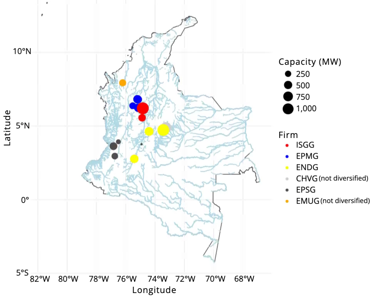
Figure 8: Dam locations

Notes: The location of Colombia dams by firm (color) and capacity (size). Colombia’s West border is with the Pacific Ocean while rivers streaming East continue through Brazil and Venezuela. To give a sense of the extension of Colombia, its size is approximately that of Texas and New Mexico combined.

Strategic firms. We consider all firms with at least a dam as strategic. For these firms, the actual value of holding water results in a trade-off between current and future production. To the extent that firms take into account future inflows, a firm will choose a supply schedule to maximize the sum of its current and future profits according to

$$\Pi_{it}=\mathbb{E}_{\epsilon}\left[\sum_{l=t}^{\infty}\beta^{l-t}\sum_{h=0}^{23}\pi_{ihl}(\epsilon_{h\iota})\right],$$

where the expectation is taken over the market demand uncertainty, $\epsilon_{ht}$, and $\beta\in(0,1)$ is the discount factor. Using a recursive formulation, a firm’s objective function becomes

$$V(\textbf{w}_{t})=\mathbb{E}_{\epsilon}\left[\sum_{h=0}^{23}\pi_{iht}+\beta\int_{\mathbb{W}}V(\textbf{u})\,f\left(\textbf{u}\big{|}\mathbf{\Omega}_{t}\right)\,\textnormal{d}\textbf{u}\right],$$ (9)

where vectors are in bold font. The state variable is the vector of water stocks, $\textbf{w}_{t}$ with domain $\mathbb{W}\equiv\{\mathcal{W}_{i}\}^{N}_{i}$, and transition matrix $f(\cdot|\mathbf{\Omega}_{t})$ following (8). The inputs in $\mathbf{\Omega}_{t}$ are the water stocks, the realized hydropower productions, and the water inflows on day $t$.

Competitive fringe. As in Section 4, the supply schedules of fringe firms is zero for prices below their marginal cost. They supply all their capacity for higher prices.

5.1 Market Power and Market Prices with Diversified Firms

In this section, we derive the optimal quantity bid submitted by generator $j$ of firm $i$. Our focus on quantity bids is grounded on the fact that generators submit hourly quantity bids but only daily price bids, providing greater flexibility in selecting quantities than price bids. We then study how market power affects pricing with differentiated firms.

Generators’ supply schedules are characterized by step functions, which makes them not differentiable (Kastl, 2011). To study the FOCs from (9), we smooth supply schedules for each firm following Wolak (2007) and Reguant (2014) (see Appendix E for the smoothing procedure). We analyze the change in discounted profits for firm $i$ resulting from a marginal change in generator $j$’s quantity bid, $q_{ijht}$, where $j$ is either a hydro ($\tau_{ij}=H$) or thermal ($\tau_{ij}=T$) generator. Omitting the expectation with respect to $\epsilon$ and the firm and generator indices ($ij$) of technology $\tau_{ij}$ for clarity, the FOCs are:

$$\frac{\partial V(\textbf{w}_{t})}{\partial q_{ijht}}=0\,:\,\, \underbrace{\left(p_{ht}\frac{\partial D^{R}_{iht}}{\partial p_{ht}}+D^{R}_{iht}\right)\frac{\partial p_{ht}}{\partial q_{ijht}}-\frac{\partial p_{ht}}{\partial q_{ijht}}\left(QC_{ijht}+\mathds{1}_{\{p_{ht}>\overline{p}\}}\overline{q}_{ijt}\right)}_{\text{Marginal revenue}}$$

$$-\underbrace{\sum_{\tau\in\{H,T\}}\left(\frac{\partial S_{iht}^{\tau}}{\partial q_{ijht}}+\frac{\partial S_{iht}^{\tau}}{\partial p_{ht}}\frac{\partial p_{ht}}{\partial q_{ijht}}\right)c^{\tau}_{it}}_{\text{Marginal cost}}$$ (10)

$$+\underbrace{\left(\frac{\partial S_{iht}^{H}}{\partial q_{ijht}}+\frac{\partial S_{iht}^{H}}{\partial p_{ht}}\frac{\partial p_{ht}}{\partial q_{ijht}}\right)\int_{\mathbb{W}}\beta\,V(\textbf{u})\frac{\partial f(\textbf{u}|\mathbf{\Omega}_{t})}{\partial S_{iht}^{H}}\textnormal{d}\textbf{u}}_{\text{Marginal value of holding water}}$$

$$+\underbrace{\sum_{k\neq i}^{N}\frac{\partial S_{kht}^{H}}{\partial p_{ht}}\frac{\partial p_{ht}}{\partial q_{ijht}}\int_{\mathbb{W}}\beta\,V(\textbf{u})\frac{\partial f(\textbf{u}|\mathbf{\Omega}_{t})}{\partial S_{kht}^{H}}\textnormal{d}\textbf{u}}_{\text{Marginal value from competitor $k$'s holding water}}\;\;=\;\;0.$$

The derivative of firm $i$’s current revenues from (7) with respect to $q_{ijht}$ is in the first line of (5.1). The first term in parenthesis is the marginal revenue in the spot market. Market power lowers marginal revenues below market prices, $p_{ht}$, if $\frac{\partial p_{ht}}{\partial q_{ijht}}<0$. Conversely, if the firm is a price taker ($\frac{\partial p_{ht}}{\partial q_{ijht}}=0$), it is paid precisely $p_{ht}$ on its marginal unit. This capacity channel prompts firm $i$ to reduce $q_{ijht}$ for all its technologies when market power increases, akin to the capacity effect witnessed in Panel (b) of Figure 4, in which market power resulted from an exogenous capacity transfer. The second term in the same line addresses how the forward contract position and the reliability payment system influence bidding in the spot market.

Market power affects equilibrium outcomes also through an efficiency channel. The actual marginal cost is the sum of its operating marginal costs, $\{c^{H},c^{T}\}$, in line two, and its intertemporal opportunity cost, in the remaining lines of (5.1), which endogeneizes the firm’s capacity constraint through a tradeoff between current and future production. By allocating more capacity to the current hydro supply, this tradeoff intensifies as it decreases the firm’s future water stock and profits. Hence, the integral in line three of (5.1) is non-positive. Since $c^{\tau}$ is constant over time, this intertemporal opportunity cost contracts or expands $i$’s cost curve for different realizations of $\mathbf{\Omega}_{t}$ setting the firm under scarcity when $\frac{\partial f(\textbf{u}|\mathbf{\Omega}_{t})}{\partial S_{iht}^{H}}<0$, or abundance when $\frac{\partial f(\textbf{u}|\mathbf{\Omega}_{t})}{\partial S_{iht}^{H}}=0$.

Generator $j$ adjusts its response to scarcity based on its market power. In the absence of market power, when $\frac{\partial p_{ht}}{\partial q_{ijht}}=0$, the firm experiences a decrease in its future profits that its equal to the change in the water stock, $\frac{\partial S_{iht}^{H}}{\partial q_{ijht}}>0$, times the expected change in future profits as in the integral in line three. The introduction of market power, denoted as $\frac{\partial p_{ht}}{\partial q_{ijht}}<0$, counteracts this loss. With market power, the firm recognizes that increasing $q_{ijht}$ marginally decreases $p_{ht}$, resulting in a smaller portion of its hydropower supply being satisfied in equilibrium as $\frac{\partial S_{iht}^{H}}{\partial p_{ht}}\frac{\partial p_{ht}}{\partial q_{ijht}}<0$. Consequently, the two terms in parentheses in the third line of (11) exert opposing influences on marginal costs during scarcity events, leading to a net positive effect for hydropower generators, which is consistent with the drop in supply ahead of droughts in Figure 4. In contrast, thermal generators cannot directly impact the firm’s hydropower supply ($\frac{\partial S_{iht}^{H}}{\partial q_{ijht}}=0$). In this case, the net effect is negative, prompting a firm to raise its thermal supply ahead of a drought to preserve its hydropower capacity. This observation is in line with results in Figure 5.

We join these observations regarding the supplies of hydro and thermal generators in the following proposition,

Proposition 2

If a firm’s revenue function is strictly concave and twice differentiable, the marginal benefit of holding water decreases in its thermal capacity $K_{i}$, i.e., $\frac{\partial^{2}V_{i}(\cdot)}{\partial w_{i}\partial K_{i}}<0$.

Proof. See Appendix A.3. $\Box$

This proposition reveals that a firm’s hydropower production increases in its thermal capacity, which squares with the theoretical analysis in the bottom panels of Figure 4. The availability of high-cost supply eases Firm 1’s resource constraint, leading to increased hydro production. Intuitively, thermal capacity reduces future water requirements, diminishing the value of holding water now. Thus, examining the efficiency channel in isolation shows that a diversified firm’s output surpasses that of two specialized firms, each with either thermal or hydro generators.

Finally, notice that the state space includes all firms’ current water stocks, $\textbf{w}_{t}$: the last line of (5.1) considers how a change in a competitor’s hydropower generator impacts $\textbf{w}_{t}$ and, thus, $i$’s expected profits through the market clearing ($\frac{\partial S_{kht}^{H}}{\partial p_{ht}}\frac{\partial p_{ht}}{\partial q_{ijht}}\leq 0$). Because this channel does not affect firm $i$’s thermal and hydro generators differently, it does not shed light on the implications of diversified technologies, on which this paper focuses.

5.1.1 Capacity vs. Efficiency in the Data

Combining the capacity and efficiency channels described above, Figure 9 illustrates the relationship between market prices (y-axis) and the slope of a firm’s residual demand (x-axis), which is flat at 0 (indicating the firm is a price taker) and vertical at 1. In Panel (a), the focus is on scarcity periods where firm $i$ has water stocks below its 30^th percentile, whereas Panel (b) considers water-abundant periods with firm $i$’s water stock above its 70^th percentile. Each scatter plot represents the average of hour-by-day markets with similar $(x,y)$ coordinates over 100 points per firm.

Viewing variation in market power as induced by variation in the technology portfolio of the firms facing scarcity, Panel (a) reveals a U-shaped relationship between prices and market power similar to that discussed in Section 4. Efficiency dominates when market power is low, causing an initial drop in market prices as demand becomes more inelastic. As market power increases, firms opt to reduce production across all technologies, leading to higher prices due to the marginal revenue effect. In contrast, the U-shape is less pronounced in Panel (b) of Figure 9, where $\frac{\partial f(\cdot|\mathbf{\Omega}t)}{\partial S{iht}^{H}}\to 0$, reducing the dependence of future profits on current production. Interestingly, this U-shape relationship is entirely driven by the crowd out ratio, which we introduced in (5) (Appendix Figure D1).

Figure 9: A U-shaped relationship between prices and the slope of the residual demand

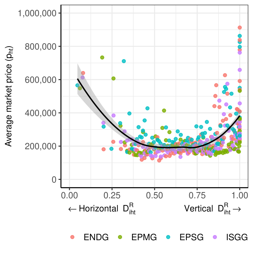
(a) Scarcity periods

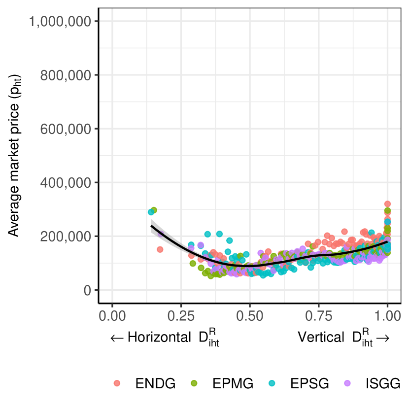
(b) Abundant periods

Notes: The figure presents binned scatter plots of the market prices (y-axis) for different slopes of a firm’s residual demand (x-axis), computed as $\frac{\partial D^{R}_{iht}}{\partial p_{ht}}\,\frac{\partial p_{ht}}{\partial q_{ijht}}$, with 100 bins per firm. Only diversified firms with dams whose bids are dispatched are considered. The black line fits the data through a spline (the 95% CI is in gray). Panel (a) focuses on markets where firm $i$ has less than the 30^th percentile of its long-run water stock. Panel (b) focuses on periods where $i$’s water stock is greater than its 70^th percentile.

5.2 Identification and Estimation

The extensive state space outlined in (5.1) presents a dimensionality challenge in estimating the relevant primitives. Existing literature offers two primary strategies to address this issue. The first method involves leveraging terminal actions (Arcidiacono and Miller, 2011, 2019), which eliminates the need to compute the value function during estimation. This approach is not applicable to our study since no exit occurred in our sample.

Our proposed solution approximates the value function with a low-dimensional function of the state space, denoted as $V(w)\simeq\sum_{r=1}^{R}\gamma_{r}\cdot B_{r}(w_{r})$, where $B_{r}(w_{r})$ are appropriately chosen basis functions. This approach echoes the work of Sweeting (2013), who introduced a nested iterative procedure. In his procedure, given an initial policy function $\sigma$ detailing the optimal course of action for each generator in a market, the algorithm (i) simulates forward the static profits $\pi_{iht}$ in (9) for $M>1$ days for each potential initial value of firm $i$’s water stock $w$ given a discount factor $\beta$, (ii) regresses the discounted sum of the $M$ daily profits on $w$ to estimate the $\gamma_{r}$ parameters of $V(w)$, and (iii) finally estimates the cost parameters in (9) given the approximated $V(w;\hat{\gamma},B)$. The iterative process halts when the implied policy from maximizing $V(w;\hat{\gamma},B)$, $\sigma^{\prime}$, is sufficiently close to the previous one. Alas, we cannot simulate forward the contribution of forward markets to current profits $\pi_{ijht}$ in step (i), as we do not observe the price of forward contracts in (7), $PC_{iht}$. Therefore, disregarding $PC_{iht}$ in the regression of discounted profits in step (ii), $\sum_{t=1}^{M}\beta^{t}\sum_{h}\pi_{ijht}(w)$, on water stocks, $w$, will not identify the $\gamma_{r}$ coefficients, as the left-hand side is a poor proxy of discounted cumulative profits, $V(w)$.

To overcome these problems, we follow Wolak (2007) and Reguant (2014) and base our analysis on the FOCs with respect to a firm’s quantity bids (5.1), which do not require knowledge of $PC_{iht}$. We rewrite (5.1) as follows:

$$\footnotesize mr_{ijht}=\sum_{\tau\in\{H,T\}}X^{\tau}_{ijht}c^{\tau}-X^{H}_{ijht}\int_{\mathbb{W}}\beta V(\textbf{u})\frac{\partial f(\textbf{u}|\mathbf{\Omega}_{t})}{\partial S_{iht}^{H}}\textnormal{d}\textbf{u}-\sum_{k\neq i}^{N}\tilde{X}^{H}_{ijht}\int_{\mathbb{W}}\beta V(\textbf{u})\frac{\partial f(\textbf{u}|\mathbf{\Omega}_{t})}{\partial S_{kht}^{H}}\textnormal{d}\textbf{u},$$ (11)

where we grouped known terms into the following variables. The left-hand side, $mr$, is the marginal revenue or the first line of (5.1). On the right-hand side, we denote the sum of the direct and indirect effects, $\frac{\partial S_{iht}^{\tau}}{\partial q_{ijht}}+\frac{\partial S_{iht}^{\tau}}{\partial p_{ht}}\frac{\partial p_{ht}}{\partial q_{ijht}}$, by $X^{\tau}$; the superscript $\tau$ indicates the technology of generator $j$, whether hidro $H$ or thermal $T$. In the last term, $\tilde{X}^{H}$ denotes the sum of the indirect effects at $i$’s competitors in the last line of (5.1). These terms and $f(\cdot|\mathbf{\Omega}_{t})$ are directly identified from the data. The only unknowns are $c^{\tau}$ and $\beta\,V(\cdot)$. Given the linearity of the FOCs, variation in $X^{\tau}$ and $\tilde{X}^{H}$ identifies $c^{\tau}$ and the coefficient vectors $\{\gamma_{r}\}_{r=1}^{R}$ approximating $V(\cdot)$. We postpone the analysis of the policy function to the next section where we run counterfactual analyses.

5.2.1 Estimation

Estimation requires fixing the number of coefficients, $R$, and the bases $B_{r}$, for approximating $V(\cdot)$. Typically, a standard spline approximation of a univariate function necessitates five bases, or knots (e.g., Stone and Koo, 1985, Durrleman and Simon, 1989). Hence, five parameters must be estimated to approximate a function in one dimension. With four firms, allowing for interactions between all the bases would require estimating $5^{4}$ parameters, which is not feasible, given that we need to instrument them. Our working assumption, echoed by the empirical results in Section 3.2.3, is that a firm only considers its future water stock when bidding. With this assumption, the transition matrix $f(\textbf{w}|\mathbf{\Omega}_{t})$ simplifies to $f(w|\mathbf{\Omega}_{t})$, and a firm’s future profits, $\beta\,V(w)$, depend on its future water stock and its law of motion (8) through $\mathbf{\Omega}_{it}$ but on $\mathbf{w}_{-it}$ only through $D^{R}_{iht}$.

We allow the transition matrix to vary across firms, $f_{i}(\cdot|\mathbf{\Omega}_{it})$. We model firm-level water inflows using an ARDL model mirroring the estimation of inflow forecasts in Section 3 (Pesaran and Shin, 1995). The unexplained portion, or model residual, informs the probability that firm $i$ will have a certain water stock tomorrow, given the current water stock and net inflows. For each firm, we fit this data with a Type IV Pearson distribution, a commonly used distribution in hydrology. This distribution’s asymmetric tails assist in exploring firms’ behaviors during water-scarce and abundant periods. Appendix B outlines the estimation of the transition matrix and discusses its goodness of fit.

Under these assumptions, the moment condition is expressed as:

$$mr_{ijht}=\sum_{\tau\in\{H,T\}}c^{\tau}X_{ijht}^{\tau}-X_{ijht}^{H}\sum_{r=1}^{5}\gamma_{r}\,\int_{\underline{w}_{i}}^{\overline{w}_{i}}B_{r}(u)\,\frac{\partial f_{i}(u|\mathbf{\Omega}_{it})}{\partial S_{iht}^{{H}}}\text{d}u+FE+\varepsilon_{ijht},$$ (12)

where we modeled $\beta\cdot V(w)\simeq\sum_{r=1}^{5}\gamma_{r}\cdot B_{r}(w_{r})$ so that no assumption about the discount factor is needed. We assume that both the marginal costs and the value functions have a non-deterministic i.i.d. component, which gives rise to the error term $\varepsilon_{ijht}$ in (12).

The estimation of $\{c^{\tau}\}_{\tau\in\{H,T\}}$ and $\{\gamma_{r}\}^{5}_{r=1}$ requires instruments as unobserved variation in supply and demand (e.g., an especially hot day) might be correlated with $X^{\tau}$. We employ variables shifting a generator’s cost to control for endogeneity. We also include various fixed effects in $FE$ to account for constant differences across firms and generators – in the real world, generators’ operating costs may differ within the hydro and thermal cathegories – and time-varying factors that affect equally all generators of a certain technology like changes in gas prices.

5.2.2 Estimation Results

We estimate (12) on daily data from January 1, 2010, to December 31, 2015. We use two-stage least squares and show the results in Table 2. We change the fixed effects used in each column. Columns (1) and (2) have fixed effects by week, while Columns (3) and (4) use daily fixed effects. Columns (2) and (4) also include month-by-technology fixed effects, in addition to fixed effects by firm, generator, and time. These adjustments help us control for seasonal factors differently affecting technologies over time.

The table has four panels. The first two panels show estimates for thermal ($c^{T}$) and hydro ($c^{H}$) marginal costs and for the five value function parameters ($\gamma_{r}$). The third panel indicates the fixed effects, whereas the last panel displays test statistics for the IVs.

Table 2: Estimated model primitives

(1) (2) (3) (4) Marginal Costs (COP/MWh) Thermal $(\psi^{thermal})$ 20,3677.62 ^∗∗∗ 141,668.46 ^∗∗∗ 22,1304.18 ^∗∗∗ 144,744.21 ^∗∗∗ (1,711.10) (1,875.29) (1,665.82) (1,561.62) Hydropower $(\psi^{hydro})$ 64,258.02 ^∗∗∗ 20,123.07 ^∗∗∗ 29,187.79 ^∗∗∗ 52,755.37 ^∗∗∗ (6,692.81) (5,309.73) (3,931.92) (3,731.31) Intertemporal Value of Water (COP/MWh) Spline 1 $(\gamma_{1})$ –2,950.20 ^∗∗∗ –6,812.77 ^∗∗∗ –11664.64 ^∗∗∗ –3,812.18 ^∗∗∗ (908.25) (528.12) (526.66) (385.60) Spline 2 $(\gamma_{2})$ –2.301e-03 ^∗∗∗ –1.546e-04 6.286e-04 ^∗∗∗ –8.402e-04 ^∗∗∗ (3.213e-04) (1.456e-04) (1.819e-04) (1.036e-04) Spline 3 $(\gamma_{3})$ –3.527e-09 ^∗∗∗ 1.919e-08 ^∗∗∗ –1.932e-08 ^∗∗∗ 1.712e-08 ^∗∗∗ (1.282e-09) (1.041e-09) (1.174e-09) (8.106e-10) Spline 4 $(\gamma_{4})$ 3.246e-08 ^∗∗∗ –3.119e-08 ^∗∗∗ 4.536e-08 ^∗∗∗ –2.729e-08 ^∗∗∗ (2.422e-09) (1.894e-09) (2.057e-09) (1.492e-09) Spline 5 $(\gamma_{5})$ –1.414e-08 ^∗∗∗ 9.357e-08 ^∗∗∗ 5.167e-08 ^∗∗∗ 8.566e-08 ^∗∗∗ (3.053e-09) (2.950e-09) (2.480e-09) (2.568e-09) Fixed Effects Firm $\checkmark$ $\checkmark$ $\checkmark$ $\checkmark$ Generator $\checkmark$ $\checkmark$ $\checkmark$ $\checkmark$ Month-by-technology $\checkmark$ $\checkmark$ Hour $\checkmark$ $\checkmark$ $\checkmark$ $\checkmark$ Week-by-year $\checkmark$ $\checkmark$ Date $\checkmark$ $\checkmark$ SW F $(\psi^{thermal})$ 194.34 162.86 1,919.25 168.62 SW F $(\psi^{thermal})$ 3,300.46 1,170.68 2,889.26 1,000.69 SW F $(\psi^{hydro})$ 458.72 267.20 877.47 360.16 SW F $(\psi^{\gamma_{1}})$ 272.15 201.92 274.58 214.83 SW F $(\psi^{\gamma_{2}})$ 220.24 266.10 266.58 292.22 SW F $(\psi^{\gamma_{3}})$ 466.55 494.96 291.98 491.58 SW F $(\psi^{\gamma_{4}})$ 570.57 577.42 292.40 566.81 SW F $(\psi^{\gamma_{5}})$ 419.44 1,156.74 432.57 920.39 Anderson Rubin F 1,213.31 1,395.05 1,527.77 1,539.08 KP Wald 143.70 142.85 138.91 147.23 N 1,451,592 1,451,592 1,451,592 1,451,592 * – $p<0.1$; ** – $p<0.05$; *** – $p<0.01$

• Notes: This table presents the coefficients obtained estimating (12) by two-stage least squares on daily data between January 1, 2010, and December 31, 2015. The top panels separate the marginal cost estimates and the value function parameters from the fixed effects used in estimation, which vary across columns. Our favorite specification is in Column (4), which includes day-fixed effects. The bottom panel provides diagnostic tests in the first stage. Robust standard errors. 2,900 COP $\simeq$ 1 US$.

Focusing on Columns (2) and (4), which control for seasonal variation by technology, we find that thermal marginal costs are about 140K Colombian pesos (COP) per MWh, or about the average price observed in the market between 2008 and 2016 (Figure 3) confirming that these units operate only during draughts, as Panel (b) of Figure 2 indicates. Consistently, the cost of operating hydropower is considerably lower, making this technology the inframarginal one. Because of the spline approximation, the $\gamma_{r}$ estimates have, instead, no economic interpretation.

Although direct comparison with other papers are challenging as engineer estimates often report the levelized cost of hydropower, which is the discounted sum of investments and operations over the lifetime of a dam, we can still compare our thermal marginal cost estimates. In USD, these estimates range between $45.57 and $70.44 per MWh in US dollars, considering fluctuations in the peso-to-dollar exchange rate over the sample period. Our findings align with other studies and engineering assessments, which typically estimate operating costs for coal-fired plants between $20 and $40 per MWh and for gas-fired plants between $40 and $80 per MWh (e.g., Blumsack, 2023).

We present several robustness checks in the appendix. First, we show that changing the number of knots to approximate $\beta\,V(\cdot)$ is inconsequential. Appendix Table D1 estimates the model using four knots instead of five and finds similar results. We also find consistent results when we use a normal distribution for the transition matrix instead of a Pearson Type IV distribution either (Appendix Tables D2 and D3).

In the next section, we use the estimated primitives to assess the price consequences of moving thermal capacity to the market leader.

6 Quantifying the Benefits of Diversification

This section first explains our simulation framework (Section 6.1) and investigates its goodness of fit (Section 6.2). Then, Section 6.3 performs counterfactual analyses by reallocating thermal capacity in the spirit of Section 4.

6.1 The Simulation Model

We base our simulation exercises on a firm’s objective function (9) because the first-order conditions in (5.1) alone are not sufficient for optimality. However, solving for the supply function equilibrium of the whole game for each firm and hourly market of the six years in our sample is computationally unfeasible. Therefore, following the approach of Reguant (2014), we construct a computational model based on (9). This model numerically determines a firm’s optimal response given the strategies of other firms in each hourly market, employing a mixed-linear integer programming solver. In essence, we evaluate the model’s performance by simulating the bids of EPMG, the leading firm in the market, while treating the bids of its competitor as given.

To ensure a global optimum, the solver requires that we discretize the technology-specific supplies over $K$ steps each. On each day $t$, the firm selects the $K$-dimensional vector of hourly quantities $\{\textbf{q}^{\tau}_{ht,k}\}_{h=0}^{23}$ for each technology $\tau$ (hydro or thermal) to solve:

$$\max_{\left\{q_{ht,k}^{\tau}\right\}_{k,h,\tau}^{K,23,\mathcal{T}}}\;\;\;\sum_{h=0}^{23}\Big{[}GR(\bar{D}_{ht}^{R})-\sum_{\tau\in\{H,T\}}\sum_{k=1}^{K}{\hat{c}^{\tau}}q_{ht,k}^{\tau}\Big{]} +\beta\sum_{m=1}^{M}\mathbb{E}\hat{V}_{t+1,m}(w_{t+1}|w_{t},\sum_{k=1}^{K}\sum_{h=1}^{23}q_{ht,k}^{H}),$$

$$s. t.$$

[Market-clearing:] $$\,\,\,\bar{D}_{ht}^{R}(p_{ht})=\sum_{\tau\in\{H,T\}}\sum_{k=1}^{K}q_{ht,k}^{\tau},\,\,\,\textnormal{$\forall\;h$},$$ (13)

[Constraints on residual demand steps:] $$\,\,\,0\leq D_{ht,z}^{R}(p_{ht})\leq\sum_{\tau\in\{H,T\}}cap^{\tau}_{ht}/Z,\,\,\,\textnormal{$\forall\;h,z$},$$

[Constraints on supply steps:] $$\,\,\,0\leq q_{ht,k}^{\tau}\leq cap^{\tau}_{ht}/K,\,\,\,\textnormal{$\forall\;h,\tau,k$},$$

[Constraints on value function steps:] $$\,\,\,0\leq\mathbb{E}\hat{V}_{t+1,m}\leq cap^{H}_{ht}/M,\,\,\,\textnormal{$\forall\;h,\tau,m$}.$$

Here, we dropped the subscript $i$ because the focus is on EPMG. The gross revenue function, $GR(\bar{D}_{ht}^{R})$, is a discretized version of the static revenues in (7). It depends on $\bar{D}_{ht}^{R}(p_{ht})=\sum_{z=1}^{Z}\mathds{1}_{[p_{ht,z}\leq p_{ht}]}D_{ht,z}^{R}$, a step function composed of $Z$ steps describing how EPMG’s residual demand varies with the market price, $p_{ht}$. The cost function is equal to the cost of producing $\sum_{k}q^{\tau}_{ht,k}$ MWh of energy using the technology-specific marginal costs estimated in Column (4) of Table 2. The remaining term of (6.1) is the expected value function, which depends on the water stock at $t$, the total MW of hydro generation produced in the 24 hourly markets of day $t$, the transition matrix, and the value function parameters $\hat{\gamma}_{r}$ estimated in Section 5.2.2. We discretize the value function over $M$ steps.

Our main focus is on the intertemporal allocation of production capacity across technologies during prolonged extreme events. Therefore, rather than simulating each daily market from 2010 to 2015, we aggregate the daily data across weeks and hours. We then determine EPMG’s optimal response using (6.1) for each hour-week combination. This strategy significantly reduces computation time while maintaining precision, as we demonstrate next.

6.2 Model Fit

In Figure 10, we compare the observed average weekly prices (red line) with the simulated ones (blue line). The model demonstrates remarkable accuracy in reproducing price volatility, particularly over the initial four years. However, the occurrence of El Niño in 2016, an unprecedented dry spell in our sample, likely influenced the transition matrix in late 2015, resulting in a gap between simulated and observed prices. While the model does not capture the extreme spike observed in late 2015, where prices surged by over tenfold, it does predict a five to sevenfold increase. Appendix Table F1 examines price variation across hours, further demonstrating a strong fit. Overall, despite being very parsimonious – using only seven parameters – the computational model effectively reproduces price volatility in Colombia over a long period.

Figure 10: Model fit: simulated (red) vs. observed prices (blue)

Note: Comparison between observed (blue) and fitted (red) prices from solving EMPG’s profit maximization problem (6.1). The solver employs ten steps to discretize the residual demand, the supply, and the value function ($M=K=Z=10$). 2,900 COP $\simeq$ 1 US$.

6.3 Counterfactual Exercises

To quantify the two sources of market power introduced in 4, this section simulates market prices by varying EPMG’s thermal capacity through capacity transfers from its competitors. Using the computational model (6.1), the counterfactuals slack EPMG’s thermal capacity constraint and affect its residual demand. Note that the estimated value function parameters ($\{\gamma_{r}\}_{r=1}^{R}$) might vary under different industry configurations if we viewed them as equilibrium objects. To solve for the new parameters, we would need to observe the counterfactual quantity submitted, which is unfeasible. However, if we could solve for the new equilibrium parameters ($\{\gamma^{\prime}_{r}\}_{r=1}^{R}$), Proposition 2 suggests that the marginal benefit of holding water decreases with a firm’s thermal capacity: we would expect EPMG to offload even more water than our counterfactual predicts for every possible demand realization, meaning lower prices on average. Therefore, this counterfactual analysis is identified in the spirit of Kalouptsidi et al. (2021).

Figure 11 summarises the results from the counterfactual exercises. In Panel (a), we move capacity from fringe firms (i.e., all the firms with no dams). The generators of these firms submit positive quantity bids for prices equal to their marginal cost: when we transfer $\kappa\%$ of generator $k$’s capacity, we do not update generator $k$’s supply if its unused capacity is large enough. Otherwise, we reduce $k$’s quantity bid accordingly. We transfer capacity from all firms in Panel (b), including EPMG’s strategic competitors. Theoretically, we should update the bids of the strategic firms in every scenario according to (6.1), but it is computationally infeasible. However, because of strategic complementarities in bidding (see Section 4), price changes can be interpreted as lower bounds for the magnitude of the actual price drop (increase) when EPMG expands (reduces) its supply after a change in its thermal capacity. For this reason, we do not investigate overall price changes from a transfer but rather focus on quantifying the scarcity / abundance scenarios from Section 4.

Each panel displays a heatmap depicting market rankings based on the severity of drought experienced by EPMG on the $x$-axis (categorized into deciles of its water stock) and the magnitude of capacity transfer on the $y$-axis. Each cell within the heatmap illustrates the average disparity between the counterfactual and status quo market prices: darker shades of blue (red) indicate lower (higher) counterfactual prices. It’s important to note that the water stock serves as a basic measure of drought, devoid of considerations about future inflows. Appendix G provides additional robustness checks using inflows on the $x$-axis. Given that these metrics only partially capture drought occurrences, the color transition across columns does not necessarily have to be smooth.

Figure 11: The price effect of a capacity transfer to the market leader

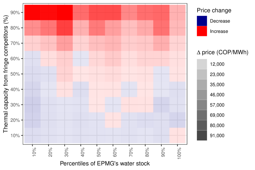
(a) Transferring $\kappa\%$ from all fringe firms

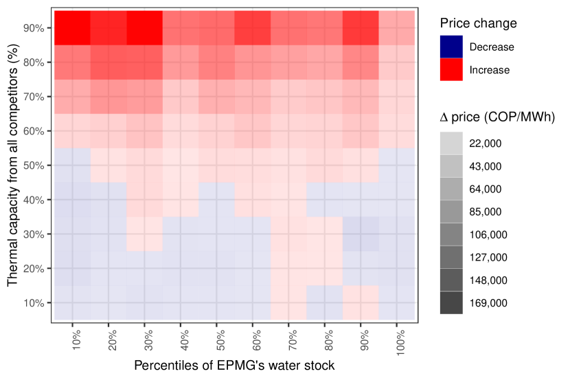
(b) Transferring $\kappa\%$ from all firms

Notes: The figure presents the results from comparing counterfactual market prices as we endow the market leading firm with greater fractions of its competitors’ thermal capacities (y-axis) for varying scarcity levels (x-axis) with baseline prices. Top (bottom) panels proxy scarcity by grouping markets based on the deciles of the firm’s water inflow (stock): each cell reports the average price difference between the simulated market and the status quo with different shades of red and blue colors based on the sign and magnitude. The left (right) panels move capacity from fringe (all) firms. The average market price is approximately 150,000 COP/MWh. 2,900 COP $\simeq$ 1 US$.

Varying capacity transfers. We first compare outcomes across transfer levels – i.e., within columns. In the first row of in Panel (a), EPMG is endowed with 10% of the fringe firms’ thermal capacity. We find lower energy market prices on average across almost all periods but the highest decile. Zooming in on transfers lower than 50% to better appreciate the magnitude changes, Panels (a) and (c) of Appendix Figure G1 show that most of the price gains are in dry periods (southwest portion of the plot). Here, price gains can be substantial, reaching values between 8,000 and 13,000 COP/MWh (slightly less than 10% of the average energy price) when moving 20% to 30% of the capacity available to the fringe firms.

In contrast, counterfactual prices mostly increase for large transfers, especially in the driest periods. During these periods, EPMG behaves as the standard textbook model would predict for a non-diversified firm that faces an increasingly vertical residual demand: it lowers output, leading to higher prices. Hence, prices first decrease for low transfers and reach a bottom level before increasing for higher transfers – a similar pattern to that observed in Panel (b) of Figure 4 where the capacity channel dominates the efficiency channel at first.

Varying drought severity. We now turn to comparing outcomes across drought severity – i.e., within rows. Panel (a) suggests a diagonal division between red and blue areas running South East (abundance and low transfers) from the North West side of the plot (scarcity and high transfers). Zooming in again on transfers smaller than 50% in Appendix Figure G1, we find that, given a transfer decile (row), cells become gradually less blue, and especially so in the first row (10% transfer). Thus, the gains from the transfers are generally larger in dry spells compared to wet periods.

Percentage price changes. A 10,000 COP price increase during drought is very different compared to a similar change during an abundant period, where prices are lower. To better compare prices across columns, we rebase the difference between counterfactual and simulated prices by the latter and present its average value in each cell (i.e., $\frac{1}{H\cdot T}\sum_{h,t}^{H,T}\frac{p^{\kappa\%}_{ht}-p^{base}_{ht}}{p^{base}_{ht}}$, where superscripts $\kappa\%$ and $base$ denotes counterfactual and baseline prices, respectively). Appendix Figure G2 presents the same analysis produced above using these percentage deviations. Also after controlling for baseline market prices, there are no gains from transferring thermal capacity when the firm has a large amount of hydropower capacity, but there are gains in the order of 10% of market prices from limited reallocations of capacity during scarcity.

Reallocating from fringe or strategic firms? Finally, Panel (b) of Figure 11 investigate when the thermal capacity transfers come from all firms, including the other diversified firms. In this case, the magnitude of the price increase (gains) is larger (smaller) compared to Panel (a) as EPMG’s residual demand is now steeper. Large transfers from strategic firms reduce the capacity available to them, decreasing the extent of market competition more than if capacity transfers were from fringe firms only.

7 Concluding Remarks

Conventional wisdom holds that market power hinges on demand factors such as elasticities, while supply factors act more like benchmarks (e.g., Nocke and Whinston, 2022). Mergers, for instance, are scrutinized for potential anti-competitive effects if they are expected to exceed the claimed cost synergies. Our paper diverges from this standard narrative by placing technology at the forefront of market power analysis. We argue that firms should be viewed as portfolios of various technologies, each with its own marginal cost and production capacity, rendering them “diversified.”

Drawing from the Colombian energy sector, whose regulatory framework mandates energy suppliers to report production by technology, we demonstrate both empirically and theoretically that oligopolistic competition among diversified firms results in a trade-off between capacity and efficiency forces. On the one hand, larger firms can cover a greater portion of the market demand, incentivizing them to decrease production to raise prices. On the other, monopolistic rents may result from a technology’s relative efficiency and may push firms to crowding out competitors, thereby decreasing prices. Moreover, we show that the mere availability of multiple technologies creates complementarities within a firm, as access to less efficient technologies relaxes the capacity constraints of the efficient ones, prompting firms to increase production across the board. These findings have implications for the way we measure capital, antitrust policies, and the transition toward greener energy markets, which we discuss further in the following sections.

7.1 Remarks on Antitrust Policies with Diversified Firms

Capital, in economic models, is typically treated as a homogeneous input, representing the aggregate of all investments a firm has made since its inception (e.g., Olley and Pakes, 1996). While economists recognize this as a necessary simplification, there has been limited exploration into the implications of this assumption due to several factors. Firstly, if introducing heterogeneity merely minimizes measurement errors, the benefits might be outweighed by the loss of tractability. Secondly, data on production by technology is scarce, making it uncertain whether firms truly engage in diversified production.

Our paper addresses this gap by revealing that heterogeneous capital holds strategic significance within standard oligopoly models. Specifically, when a firm with a cheap technology but limited capacity adds a more expensive technology, the value of the cheap technology increases for the firm. As a result, the firm is willing to use more of the cheap technology to dominate the market. In response, competitors adopt aggressive pricing strategies to safeguard their market share, even if it means sacrificing revenues on marginal units.

The key takeaway from our analysis is that we should consider a broader view when we analyze market concentration. In industries with high barriers to entry where firms have significant pricing power, achieving the optimal technology mix can drive prices down more than policies focused solely on limiting firm size. For instance, Colombian regulations cap firm capacity at 25% of the industry, hindering diversification due to the scale of dam projects.

These insights also shed light on the landscape of horizontal merger policies, which traditionally rely on concentration as a primary gauge of market distortions (e.g., Benkard et al., 2021). In particular, standard tools used by antitrust agencies to curb concentration post-merger, such as divestitures, may be anti-competitive. Beyond simply reducing capacities, divestiture can also diminish firms’ diversification, thereby limiting their ability to respond to scarcity events like periods of high input costs. This could trigger less aggressive pricing from competitors and lead to higher market prices.

Our findings are not driven by standard synergies typically associated with merging parties benefiting from economies of scale or scope. For example, it is common to model the marginal cost of a merger between two firms, each with costs $c^{a}$ and $c^{b}$, as $\min\{c^{a},c^{b}\}$, often attributed to improved managerial practices (e.g., Braguinsky et al., 2015, Demirer and Karaduman, 2022) or technological advancements (e.g., Ashenfelter et al., 2015, Miller and Weinberg, 2017). However, in our framework, “synergies” come from equilibrium responses rather than from economies of scale or scope. These synergies are similar to those seen in mergers of multiproduct firms, as described by (Nocke and Schutz, 2018a). In such mergers, the markup that the merged company charges for a specific product reflects demand elasticity and the cannibalization effects across its other various products. Similarly, our equation shows that a firm’s markups, when selling a homogeneous product from multiple technology, depend on demand elasticity and crowding-out incentives created by the opportunity to undercut competitors with one specific technology.

We believe that our model and results are widely applicable. Firstly, based on Klemperer and Meyer (1989)’s discussion, we believe our model and insights can be effectively applied to multi-product firms. Second, our model operates on the premise of uncertain demand, with firms committing to a supply curve before demand is realized. In reality, large firms are likely to have some private information about their residual demand, and the quantity supplied will depend on this information. So effectively, firms do commit to a supply curve, and hence, our model also applies to other industries where firms are diversified across multiple technologies. For example, Collard-Wexler and De Loecker (2015) studies various methods for alumina production, while labor inputs may also exhibit diverse efficiency – based on worker types – and capacity – based on total headcounts – (e.g., Bonhomme et al., 2019).

7.2 Remarks on the Green Transition with Diversified Firms

The energy sector is responsible for a large share of global CO₂ emissions (IEA, 2023), necessitating a transition to less-carbon-intensive technologies such as renewables (e.g., Elliott, 2024). While renewables are generally inexpensive, their intermittent nature can lead to high prices during periods of scarcity. As energy prices, like those of other utilities, decrease consumers’ disposable income, disproportionately affecting low-income consumers (Reguant, 2019, Haar, 2020), the energy transition might widen current inequality trends, highlighting the need for governmental agencies to actively manage and mitigate high energy price scenarios during the transition.

To encourage generators to produce more during scarcity events, governments have implemented policies like the reliability charge outlined in Section 5. These policies require generators to produce a set amount of energy when prices rise above a certain threshold, with subsidies as incentives. However, these subsidies are costly and can provide incentives to firms with market power to increase prices to access the subsidies (McRae and Wolak, 2020).

The question of ownership of the means of production has long been contentious in transitioning economies (e.g., Murphy et al., 1992), and the pursuit of the green transition is no exception. In this context, our research introduces a novel approach to tackle intermittencies in the energy sector by leveraging ownership links. We find that generators unaffected by scarcity can absorb the scarcity experienced by renewable generators owned by the same firm, especially when the firm holds market power. While perfect competition would ideally lead to the first-best outcome, this might be hard to enforce by policymakers because the marginal cost of a renewable generator is the sum of operating costs and intertemporal opportunity costs, which might be unknown to policymakers. Thus, our results suggest policymakers can look for the optimal level of diversification within firms instead to lower energy prices. Our analysis suggests that transferring non-renewable capacity to a firm anticipating a drought could reduce price spikes by around 5 to 10% (see Appendix Figure G2), as these generators internalize scarcity periods at sibling dams, a meaningful reduction particularly during drought periods with little cost during abundance periods.

In Colombia, hedging against energy scarcity predominantly relies on fossil fuels, contributing to increased CO₂ emissions and impeding the transition to green energy. This reliance stems from the geographical concentration of dam ownership, a legacy of privatizations in the 1990s. Had dam ownership been more diversified across regions – as opposed to the ownership structure depicted in Figure 8 – reliance on dams with varying inflow seasonality could have provided an alternative form of hedging, potentially reducing emissions and enhancing welfare compared to the current situation.

As of 2024, Colombia’s renewable energy capacity from solar and wind sources remains limited, constituting only 1.5% of the total installed capacity. However, there were notable developments, with twelve wind projects totaling 2,072 MW and six solar projects totaling 908 MW under construction by the end of 2022. Additionally, the Colombian governmental agency responsible for natural resource management, Unidad de Planeación Minero Energética, approved several other solar and wind farm projects set to commence operations by 2027 (Arias-Gaviria et al., 2019, Rueda-Bayona et al., 2019, Moreno Rocha et al., 2022). Once operational, these projects are projected to contribute approximately 38% of Colombia’s installed capacity (SEI, 2023). With ongoing advancements in storage technology and declining battery costs (Koohi-Fayegh and Rosen, 2020), renewables are poised to emerge as a more cost-effective alternative to fossil fuels for hedging against energy scarcity, particularly for hydropower.

Diversified firms are well-positioned to internalize scarcity efficiently. Further investments in renewable energy infrastructure and a well-designed ownership structure promise to facilitate a swift and economical transition toward a greener economy.

Prices and Concentration: A U-shape?
Theory and Evidence from Renewables

Michele Fioretti                   Junnan He                   Jorge Tamayo

Online Appendix

Part Online Appendix

Appendix A Theoretical Appendix

Appendix A.1 defines supply function equilibria and derives the FOCs using ex post optimization. Appendix A.1.1 analyze an asymmetric duopoly for which we can assess the impact of technology reallocation analytically. These counterfactual analysis are in Appendices A.1.2, with proofs in A.2.2, and A.2.3. Appendix A.1.3 solves for a different counterfactual where firms are symmetric and have access to both technologies. Appendix A.2.1 hosts a set of lemmas and proofs for the existence and uniqueness of the SFE.

Appendix A.3 proves Proposition 2, which we introduced in the structural model in Section 5. It demonstrates that the marginal benefits of holding water decrease in a firm’s thermal capacity.

A.1 Theoretical Model of Section 4

An industry has $N$ firms producing a homogeneous good. The industry demand is inelastic $D$ and is subject to an exogenous shock $\epsilon$, where $\epsilon$ is a random variable and that $D(\epsilon)>0$ can take any positive value. The $\epsilon$ can be a horizontal translation of $D$ as in klemperer1989supply.

Assume that Firm $i\in\{1,...,N\}$ has total cost function $C_{i}(S)\geq 0$ when $i$ produces $S$ units of goods. Intuitively, when $S$ is larger than $i$’s capacity, the cost of production becomes $\infty$.

A strategy for firm $i$ is a non-decreasing, left-continuous, and almost everywhere differentiable function mapping prices to a maximum level of output for that price, i.e., $S_{i}(p):[0,\infty)\to[0,\infty)$. Firms choose their supply functions simultaneously without knowledge of the realization of $\epsilon$. The market price, $p^{*}$, is the smallest $p$ such that $D(\epsilon)$ is satisfied. That is, industry demand matches industry supply according to the market clearing condition:

$$p^{*}(\epsilon):=\min\left\{p\in[0,\infty)\text{ such that }\sum_{j}S_{j}(p)\geq D(\epsilon)\right\}.$$ (A1)

The minimum is well defined for $S_{i}$ are non-decreasing and left-continuous. We denote $p^{*}(\epsilon)$ simply by $p^{*}$ to reduce notation from now on.

After the realization of $\epsilon$, supply functions are implemented by each firm producing at $(p^{*},S_{i}(p^{*}))$. Firm $i$ sells $S_{i}(p^{*})$ and gets $p^{*}$ on each unit it sells. Its profit is

$$\pi_{i}(p^{*})=p^{*}\cdot S_{i}(p^{*})-C_{i}(S_{i}(p^{*})).$$ (A2)

We denote $i$’s residual demand as $D^{R}_{i}(p,\epsilon)\equiv\max\{0,D(\epsilon)-\sum_{j\neq i}S_{j}(p)\}$. In equilibrium (to be defined next), $i$’s quantity supplied equates to its residual demand at the market clearing $p^{*}$, i.e. $S_{i}(p^{*})=D^{R}_{i}(p^{*},\epsilon)$. Hence, firm $i$’s ex post profit is equivalently

$$\pi_{i}(p^{*})=p^{*}\cdot D^{R}_{i}(p^{*},\epsilon)-C_{i}(D^{R}_{i}(p^{*},\epsilon)).$$ (A3)

Ex post optimization. As in klemperer1989supply, the ex post profit-maximizing level of production for each firm depends on the realization of its residual demand curve. Given the strategy of the other firms, the residual demand curve for $i$ changes as $\epsilon$ varies. Given each $\epsilon$ if there is a profit maximizing level of production $q_{i}$ with an associated market clearing price level $p$. As $\epsilon$ varies, these two quantity can be described by a supply function $q_{i}=S_{i}(p)$. It can be seen that by committing to $S_{i}$, $i$ can achieve ex post optimality for every realization of the demand.

Definition A.1

Supply Function Equilibrium (SFE). An equilibrium is an $N$-tuple of functions $(S_{l}(p))_{l=1}^{N}$ such that given each firm $j\neq i$ chooses $S_{j}(p)$, for every realization of $\epsilon$, $S_{i}(p^{*})=D^{R}_{i}(p^{*},\epsilon)$ for which $p^{*}$ maximizes $i$’s ex post profit in (A3).

FOCs using ex post optimality. The ex post optimality can be obtained when $i$ solves at every $\epsilon$:

$$\max_{p}\pi_{i}(p):=p\cdot\Big{(}D(\epsilon)-\sum_{j\neq i}S_{j}(p)\Big{)}-C_{i}(D^{R}_{i}(p,\epsilon)),$$ (A4)

which admits the following FOCs almost everywhere with $i$ supplying positive quantity,

$$p\frac{\partial D_{i}^{R}(p,\epsilon)}{\partial p}+D_{i}^{R}(p,\epsilon)-C_{i}^{\prime}\cdot\frac{\partial D_{i}^{R}(p,\epsilon)}{\partial p}=0\Longleftrightarrow\left(p-C_{i}^{\prime}\right)S_{-i}^{\prime}(p)=S_{i}(p),$$ (A5)

where the second equality follows from market clearing $S_{i}=D^{R}_{i}(p,\epsilon)$ and we use $S_{-i}(p):=\sum_{j\neq i}S_{j}(p)$. If for instance, (A3) is globally strictly concave in $p$, then (A5) implicitly determines $i$’s unique profit maximizing price $p_{i}^{*}(\epsilon)$ for each value of $\epsilon$. The corresponding profit maximizing quantity is $D(\epsilon)-\sum_{j\neq i}S_{j}(p^{*}_{i}(\epsilon))\equiv q^{*}_{i}(\epsilon)$.

From (A5), one can observe that when $C^{\prime}_{i}=c_{i}$ on some open interval of production levels, the model exhibits strategic complementarities and the markup reflects the elasticity of demand and a crowding out ratio.

Proposition 3

Strategic complementarities. When $C^{\prime}_{i}=c_{i}$, $i$’s best response $S_{i}$ to $S_{-i}$ is increasing in $S_{-i}^{\prime}$, and $S_{i}^{\prime}$ is increasing in the level of $S_{-i}^{\prime}$.

It follows immediate from (A5) and its total derivative w.r.t. $p$: $\left(p-c_{i}\right)S_{-i}^{\prime\prime}+S_{-i}^{\prime}=S_{i}^{\prime}.$

Clearly, firms react by bidding more aggressively (increase both $S_{i}$ and $S_{i}^{\prime}$) when opponents bid more aggressively (increase $S_{-i}^{\prime}$ to $S_{-i}^{\prime}+constant$). Hence, both the intercept and the slope of $S_{i}(p)$ increase with the supply of the competitors, resulting in strategic complementarity.

Proposition 4

Crowding-out ratio. Firm $i$’s markup satisfies $\frac{p-C_{i}^{\prime}}{p}=\frac{s_{i}}{\eta}\cdot\left(\frac{S^{\prime}_{i}(p)}{-{D^{R}_{i}}^{\prime}(p)}+1\right),$ where $s_{i}$ is its market share, and $\eta$ is the price elasticity of demand. The crowding-out ratio is $\frac{S^{\prime}_{i}(p)}{-{D^{R}_{i}}^{\prime}(p)}+1$.

This proposition follows immediately from (A5). Denote $S(p):=\sum_{j=1}^{N}+S_{j}(p)$ and $s_{i}:=\frac{S_{i}(p)}{S(p)}$, rewrite (A5) as

$$\frac{p-C_{i}^{\prime}}{p}\cdot\underbrace{\left(\frac{S^{\prime}(p)}{S(p)}\cdot p\right)}_{\eta}\cdot\frac{S_{-i}^{\prime}(p)}{S^{\prime}(p)}=\underbrace{\frac{S_{i}(p)}{S(p)}}_{s_{i}}\Leftrightarrow\frac{p-C_{i}^{\prime}}{p}=\frac{s_{i}}{\eta}\cdot\left(\frac{S^{\prime}_{i}(p)}{-{D^{R}_{i}}^{\prime}(p)}+1\right)$$

where we obtain the price elasticity of demand $\eta$ using the identiy $S(p)=D(\epsilon)$. In particular, we have $S^{\prime}(p)\cdot\frac{dp}{dD}=1$, and hence $S^{\prime}(p)=\frac{dD}{dp}$. Define $\eta$ as $S^{\prime}(p)\cdot\frac{S(p)}{p}$, then $\eta=\frac{dD}{dp}\cdot\frac{S(p)}{p}=\frac{dD}{dp}\cdot\frac{D}{p}$ by market clearing. Hence $\frac{1}{\eta}=\frac{dp}{dD}\cdot\frac{p}{D}$ is the price elasticity of demand.

A.1.1 Duopoly Competition with Analytical Solutions

We now specifies the two cases studied in the main text using the theoretical framework above, and then analytically solve for the equilibrium.

Costs. Firms have access to three types of technologies, high-, low-, and fringe-cost, such that $c^{l}<c^{h}<c^{f}$. The technology set is $\mathcal{T}=\{l,h,f\}$. The total cost of firm $i$ is $C_{i}\equiv\sum_{\tau\in\mathcal{T}}c^{\tau}S_{i}^{\tau}(p)$, where we denote $i$’s supply with technology $\tau$ by $S_{i}^{\tau}(p)$. Firm $i$ has a given capacity of each technology $K_{i}^{\tau}$, so that $S_{i}^{\tau}\in[0,K_{i}^{\tau}]$. Notice that due to the merit order, each firm always supply with the cheapest technology before adopting the more expensive ones. Therefore at every total quantity of production, there is a unique cost-minimizing production allocation to each technology within a firm. So there is a one-to-one correspondence between (the cost minimizing) total supply function of a firm and the tuple of supply function by technologies, that $S_{i}(p)=\sum_{\tau\in\mathcal{T}}S_{i}^{\tau}(p)$.

Capacities. A firm is described by a technology portfolio, that is a vector $K_{i}=(K_{i}^{l},K_{i}^{h},K_{i}^{f})$, describing the capacity available to firm $i$ for each technology.

Baseline capacities. In general, all the capacities are non-negative. We will focus on the setting where Firm 1’s technology portfolio is $K_{1}=(K_{1}^{l},K_{1}^{h},0)$, where $K_{1}^{h}$ is either 0 as in Section 4 or a small enough number (to be defined in the proof of Appendix A.2.3, Firm 2’s technology portfolio is $K_{2}=(0,K_{2}^{h},0)$, and non-strategic (fringe) firm $i$’s technology portfolio for $i\in(3,...,N)$ is $K_{i}=(0,0,K_{i}^{f})$. We also assume that $K_{i}^{f}$ is of negligible size for all fringe firms, and hence these fringe firms will behave competitively.

Counterfactual scenario. We move $\delta$ units of $K_{2}^{h}$ from Firm 2 to Firm 1. The new technology portfolios are $\tilde{K}_{1}=(K_{1}^{l},K_{1}^{h}+\delta,0)$, $\tilde{K}_{2}=(0,K_{2}^{h}-\delta,0)$, and $\tilde{K}_{i}=(0,0,K_{i}^{f})$ for $i\in(3,...,N)$ .

Demand. Demand is inelastic and subject to a shock $\epsilon$ as usual.

Market clearing. There is a large enough number of non-strategic firms. They enter the market only when the price at least covers their marginal cost, $c^{f}$. At this price, they supply all their capacity. Hence, their supply function is $S_{i}=1_{\{p>c^{f}\}}K^{f}_{i}$ for $i\in(3,...,N)$ and $\sum_{j=3}^{N}K_{j}^{f}$ is large enough, so that the market always clears for $p\geq c^{f}$.

Without loss of generality, we assume that in equilibrium, the strategic firms have priority in production over the fringe firms at price $p=c^{f}$. Hence, for any realization $D$ of $D(\epsilon)$, given the schedules $S_{i}(p)$, the market clearing price from (A1) becomes

$$p^{*}=\min\Big{\{}c^{f},\inf\big{\{}p\big{|}\sum_{i}^{N}S_{i}(p)\geq D\big{\}}\Big{\}}.$$ (A6)

Residual demand. Therefore, for $i=1,2$, Firm $i$’s residual demand function is

$$D_{i}^{R}(p,\epsilon)=\begin{cases}D(\epsilon)-S_{-i}(p),&\text{ for }p\in[0,c^{f}),\\ \min\{D(\epsilon)-S_{-i}(p),\sum_{\tau}K_{i}^{\tau}\},&\text{ for }p=c^{f},\\ 0,&\text{ for }p>c^{f},\end{cases}$$

where $S_{-i}(p)\equiv\sum_{j\neq i}S_{j}(p)$.

Profits and best responses. We update (A3) according to the new cost functions. Given the opponent’s strategy, the profit of firm $i$ with cost function $C_{i}$ at the market clearing price $p$ is

$$\pi_{i}(p)=D_{i}^{R}(p,\epsilon)\cdot p-\sum_{\tau\in\mathcal{T}}c^{\tau}S_{i}^{\tau}(p).$$ (A7)

Following the definition of an SFE (A.1), in this duopoly context, an SFE is a pair of supply functions $S_{i}(p)=\sum_{\tau}S_{i}^{\tau}(p)$ for $i\in\{1,2\}$ that maximizes the ex post profit (A7) for each $i$ at every possible level of $D(\epsilon)$ and for which the price $p$ clears the market. Moreover, Each non-strategic firm, being a marginal player, sell its entire capacity whenever $p\geq c^{f}$ and do not produce otherwise.

The following lemmas are useful to compute the SFE, on which we turn next.

Lemma A.1: in equilibrium, the supply functions are strictly increasing on $(c^{h},c^{f})$ and no firm exhausts its total capacity for $p<c^{f}$. Intuition: when such $p$ is realized, the constrained firm can reduce production by $\epsilon$, causing the price to have a discrete jump to $c^{f}$, a profitable deviation.

Lemma A.2: one of the two firms will exhaust its capacity as $p\to c^{f}$ from below. Intuition: If both firms do not exhaust their capacity at $c^{f}$, one of them can deviate and choose to exhaust the capacity at price $c^{f}-\epsilon$ to engage in a Bertrand style competition to increase its profit.

Lemma A.3: production decisions based on the merit order are optimal (i.e., a diversified firm first exhausts its low-cost capacity before moving to the high-cost one).

Lemma A.4: supply functions are differentiable almost everywhere for $p\in(c^{h},c^{f})$. Intuition: $(S_{i}(p))_{i=\{1,2\}}$ are the solutions of a system of differential equations that are increasing and continuous. The only point where $S_{i}(p)$ is not differentiable is at $\hat{p}$ s.t. $S_{1}(\hat{p})=S_{1}^{l}(\hat{p})=K_{1}^{l}$, that is the price at which Firm 1 exhausts its low-cost capacity and starts producing with its high-cost capacity.

Lemma A.5: technical step proving that the conditions under which the equilibrium supply functions computed in the next section are unique.

With the above Lemmas, one can show that an SFE exists and is unique.

Proposition 5

The duopoly competition defined in Appendix A.1.1 has a unique SFE.

We postpone the proofs of the Lemmas and the Proposition to Appendix A.2.1. Below we study the comparative static of relocating capacities from Firm 2 to Firm 1 and its effect on market prices.

A.1.2 Reallocation of Capacities

We consider a small capacity reallocation $\delta>0$ from Firm 2 to Firm 1, so that the new technology portfolios become $\tilde{K}_{1}=(K_{1}^{l},K_{1}^{h}+\delta,0)$, $\tilde{K}_{2}=(0,K_{1}^{h}-\delta,0)$, and $\tilde{K}_{l}=(0,0,K_{l}^{f})$ for fringe firm $l=(3,...,N)$.

Proposition 1 A marginal capacity transfer from Firm 2 to Firm 1 increases the equilibrium price if $K_{1}^{l}>\frac{c^{f}-c^{l}}{c^{f}-c^{h}}K_{2}^{h}$ (abundance scenario) and decreases it if $K_{1}^{l}<\frac{c^{f}-c^{l}}{c^{f}-c^{h}}K_{2}^{h}$ (scarcity scenario).

We prove the part relating the abundance scenario in Appendix A.2.2 and the part relating to the scarcity scenario in Appendix A.2.3.

To understand the proof of Proposition 1, observe that Firm 1 has a dominating capacity in the abundance scenario. Reallocating $\delta$ capacity to Firm 1 exacerbates its position of market power vis-à-vis Firm 2. As Firm 2 exhausts its capacity as $p\to c^{f}$ from below, the proof shows that Firm 1 uses the $\delta$ capacity only for $p=c^{f}$. Effectively, the transfers remove capacity from the market for $p\in(c^{h},c^{f})$, leading to higher prices for non-extreme realizations of $D(\epsilon)$. That is, Firm 1 gains from the inframarginal units sold at a higher market price. The same proof can be used to show that the analogous result holds when there is no diversification. Any reallocation from the smaller firm to the larger firm when both own the same technology increases the market price.

On the other hand, a marginal transfer of $\delta$ in the scarcity scenario incentivizes the Firm 1 to employ its low-cost technology to crow-out Firm 2 for every realizations of $D(\epsilon)$. The proof shows that in this situation, Firm 1 exhausts all its capacity before Firm 2 as $p\to c^{f}$ from below. Hence the $\delta$ greater capacity slacks the cost constraint faced by Firm 1, and Firm 1’s equilibrium supply schedule expands after the transfer. Firm 2’s supply expands as well because of strategic complementarity (Section A.1). We call these two forces the “crowding out” incentives. Loosely speaking, they arise because SFEs include Bertrand competition as an extreme case.

Figure A1: Supplies of Firm 2 and fringe firms before and after the transfer

(a) Abundance scenario
$K_{1}=(9,0,0)\,\&\,K_{2}=(0,4,0)$

(b) Scarcity scenario
$K_{1}=(5,0,0)\,\&\,K_{2}=(0,4,0)$

Notes: Each panel illustrates the equilibrium supply of Firm 2 and the supply of fringe firms (gray dotted lines) under abundance in Panel (a) and scarcity in Panel (b) using the parameters as in Figure 4. The cost of Firm 2 is the dotted blue line. Solid (shaded) lines refer to Firm 2’s costs and supply after (before) the capacity transfer of 0.5 units from Firm 2 to Firm 1.

A.1.3 Reallocation Under Symmetry

This section studies a similar capacity reallocation of high-cost technologies from Firm 2 to Firm 1 under the case where both Firm 1 and Firm 2 have the same technology portfolio $K_{1}=K_{2}=(K^{h},K^{l},0)$. The technology portfolio of the fringe firms stay unchanged.

Proposition 6

In the duopoly competition defined in Section A.1.3, a marginal capacity transfer from Firm 2 to Firm 1 increases the market price.

The proof is in Appendix A.2.4. One can view the symmetric case as the optimal benchmark. No reallocation can increase competition in the market. Indeed, reallocating high-cost capacities, decreases the competitivity of one firm similar to the abundance scenario.

A.2 Proofs of Propositions and Lemmas

A.2.1 Proof of Proposition 5 (Existence and Uniqueness of the SFE)

The proof relies on the following Lemmas.

Lemma A.1

In equilibrium, $S_{i}(p)<\sum_{\tau}K_{i}^{\tau}$ for every $p<c^{f}$. Moreover, $S_{i}(p)$ is strictly increasing on the interval $(c^{h},c^{f})$.

Proof. Suppose on the contrary that firm $i$ exhausts all its capacity at some price s.t. $S_{i}(\hat{p})=\sum_{\tau}K_{i}^{\tau}$ for $\hat{p}<c^{f}$. Since $S_{i}(p)$ is right continuous, let $\underline{p}$ be the smallest such price for $i$. Then the best response of $i$’s competitor, denoted by $j$, satisfies $S_{j}(p)=S_{j}(\underline{p})$ on $p\in(\underline{p},c^{f})$. This is because if there exists $\dot{p}\in(\underline{p},c^{f})$ such that $S_{j}(\dot{p})-S_{j}(\underline{p})>0$, then $S_{j}(p)=S_{j}(\underline{p})$ is not a best response and has a profitable deviation since $j$ has capacity available and $\dot{p}>c^{h}$. In the event that this $\dot{p}$ clears the market, $j$ can benefit from deviating to produce slightly less at $\dot{p}$ and causing the market clearing price to increase. Since $\dot{p}$ is arbitrary, $S_{j}(p)=S_{j}(\underline{p})$ is the best-response of $S_{i}(p)=S_{i}(\underline{p})$.

Now, if $S_{i}(p)=S_{i}(\underline{p})$ on $p\in(\underline{p},c^{f})$ for both $i\in\{1,2\}$, then in the event where $\underline{p}$ clears the market, either firm can profitably deviate by slightly reducing production and causing the price to jump up to $c^{f}$. Hence, it is not optimal to exhaust capacity for $p<c^{f}$.

To see the second assertion, if there exist two prices $\underline{p}<\overline{p}$ in the interval $(c^{h},c^{f})$ such that $S_{i}(\underline{p})=S_{i}(\overline{p})<K_{i}$, we can apply a similar argument as above and conclude that the best response for $j$ is $S_{j}(\underline{p})=S_{j}(\overline{p})$. W.l.o.g., let $\overline{p}$ be the sup of all the prices for which this equality holds. In the case when $\overline{p}+\epsilon$ is the market clearing price for all small enough $\epsilon>0$, increasing the production at the price $\overline{p}$ is a profitable deviation for at least one of the players. $\Box$

Lemma A.2

In equilibrium, there exists $i\in\{1,2\}$ such that $\lim_{p\to c^{f-}}S_{i}(p)=\sum_{\tau}K_{i}^{\tau}$.

Proof. At least one of the firms exhausts its capacity in the left limit of $c^{f}$. This is because fringe firms enter and there will be no market for $p>c^{f}$. So any remaining capacity will be produced at $c^{f}$, that is $S_{i}(c^{f})=\sum_{\tau}K_{i}^{\tau}$ for both $i$. If both firms do not exhaust their capacity in the left limit of $c^{f}$, then both supply schedules have a discrete jump at $c^{f}$. In the event that the market demand is met at $c^{f}$ but $D(\epsilon)<\sum_{i,\tau}K_{i}^{\tau}$, one of them can deviate by exhausting its capacity at the price just epsilon below $c^{f}$ to capture more demand, a profitable deviation. $\Box$

Lemma A.3

The production cost for firm 1 at different market-clearing prices satisfies

$$C_{1}=\begin{cases}c^{l}S_{1}^{h}(p)&\text{ iff }S_{1}^{h}(p)<K_{1}^{h};\\ c^{l}K_{1}^{l}+c^{h}S_{1}^{h}(p)&\text{ iff }S_{1}^{l}(p)=K_{1}^{l}.\end{cases}$$

Proof. Since $C_{i}$ is the minimal cost function for producing a given quantity of electricity, because the marginal cost of hydro production is lower, firm 1 will necessarily first produce with hydro and only start thermal production when hydro capacity is exhausted. $\Box$

Lemma A.4

For $i\in\{1,2\}$ the function $S_{i}(p)=S_{i}^{l}(p)+S_{i}^{h}(p)$ is continuous on the interval $(c^{h},c^{f})$. It is continuously differentiable except possibly for $S_{2}(p)$ at $p$ for which $S_{1}(p)=K_{1}^{l}$.

Proof. The supply functions are non-decreasing by definition. Hence, a discontinuity of $i$’s supply at some price $p\in(c^{h},c^{f})$ is, therefore, a discrete jump in $i$’s production. In the event that such $p$ clears the market, firm $j$ has a profitable deviation to increase its production at $p-\epsilon$ for any $\epsilon$ small enough. Therefore, in equilibrium, the total supply function of each firm is continuous at every $p\in(c^{h},c^{f})$.

By Lemma A.3, it holds except for the case where $i=1$ and $S_{1}(p)=S_{1}^{l}(p)=K_{1}^{l}$, that for any small enough interval $U\subset(c^{h},c^{f})$, there exists $\tau\in\{l,h\}$, such that all $p,p^{\prime}$ on that small interval,

$$C_{i}(S_{i}(p))-C_{i}[S_{i}(p)+S_{j}(p)-S_{j}(p^{\prime})]=-c^{\tau}\left(S_{j}(p)-S_{j}(p^{\prime})\right).$$ (A8)

Now consider the case that $p\in(c^{h},c^{f})$ clears the market, firm $i$ is maximizing by producing $S_{i}(p)$ and $S_{1}(p)+S_{2}(p)=D(\epsilon)$. Therefore, any $p^{\prime}$ on the same interval satisfies

$$S_{i}(p)\cdot p-C_{i}(S_{i}(p))\geq[D(\epsilon)-S_{-i}(p^{\prime})]\cdot p^{\prime}-C_{i}[D(\epsilon)-S_{-i}(p^{\prime})],$$

that is if $i$ deviates its production so that the market clearing price changes to $p^{\prime}$, it would not be a profitable deviation. Therefore with (A8) we have

$$S_{i}(p)\cdot p-C_{i}(S_{i}(p)) \geq[S_{i}(p)+S_{-i}(p)-S_{-i}(p^{\prime})]\cdot p^{\prime}-C_{i}[S_{i}(p)+S_{-i}(p)-S_{-i}(p^{\prime})]$$

$$\Leftrightarrow$$

$$S_{i}(p)\cdot(p-p^{\prime}) \geq[S_{-i}(p)-S_{-i}(p^{\prime})]\cdot[p^{\prime}-c^{\tau}]$$

$$\Leftrightarrow$$

$$\frac{S_{i}(p)}{p^{\prime}-c^{\tau}}(p-p^{\prime}) \geq S_{-i}(p)-S_{-i}(p^{\prime}).$$

Similarly, consider market clearing at $p^{\prime}$ gives

$$\frac{S_{i}(p^{\prime})}{p-c^{\tau}}(p^{\prime}-p)\geq S_{-i}(p^{\prime})-S_{-i}(p).$$

Therefore, for any $p,p^{\prime}\in U$ with $p-p^{\prime}=\delta>0$ we have

$$\frac{S_{i}(p)}{p^{\prime}-c^{\tau}}\geq\frac{S_{-i}(p)-S_{-i}(p^{\prime})}{p-p^{\prime}}\geq\frac{S_{i}(p^{\prime})}{p-c^{\tau}}.$$

Since this holds for all $\delta$ near $0$, by continuity of $S_{i}$ (Lemma A.3) we have

$$\limsup_{\delta\to 0-}\frac{S_{-i}(p+\delta)-S_{-i}(p)}{\delta}\leq\frac{S_{i}(p)}{p-c^{\tau}}\leq\liminf_{\delta\to 0+}\frac{S_{-i}(p+\delta)-S_{-i}(p)}{\delta}.$$

which implies $S_{-i}$ is continuously differentiable on $(c^{h},c^{f})$. The only exception is when $i=1$ and $S_{1}(p)=K_{1}^{h}$, then $S_{j}(p)=S_{2}(p)$ is allowed to be non-smooth at $p$ where $S_{1}(p)=K_{1}^{h}$. $\Box$  

Lemma A.5

Using $c_{3},c_{4}$ solved in $c_{1}$ as in (A14), whenever $c_{1}\geq\frac{K_{1}^{l}}{c^{f}-c^{l}}$ we have

1. $c_{3}(c^{f}-c^{h})-c_{4}/(c^{f}-c^{h})\geq c_{1}(c^{f}-c^{h})$ where the equality holds iff $c_{1}=\frac{K_{1}^{l}}{c^{f}-c^{l}}$;

2. $c_{3}(c^{f}-c^{h})+c_{4}/(c^{f}-c^{h})\geq c_{1}(c^{f}-c^{l})$ where the equality holds iff $c_{1}=\frac{K_{1}^{l}}{c^{f}-c^{l}}$;

3. $c_{3}(c^{f}-c^{h})-c_{4}/(c^{f}-c^{h})$ and $c_{3}(c^{f}-c^{h})+c_{4}/(c^{f}-c^{h})$, as functions in $c_{1}$, are continuous and strictly increasing to $\infty$.

Proof. Item 1: Using the above notations, we have

$$c_{3}(c^{f}-c^{h})-c_{4}/(c^{f}-c^{h})-c_{1}(c^{f}-c^{h})$$

$$= \frac{c_{1}}{2}\left(1+\frac{\alpha}{\alpha-c_{1}}\right)(c^{f}-c^{h})-\frac{(c^{h}-c^{l})^{2}}{2}\frac{\alpha-c_{1}}{c^{f}-c^{h}}-c_{1}(c^{f}-c^{h})$$

$$= \frac{c_{1}}{2}\frac{c_{1}}{\alpha-c_{1}}(c^{f}-c^{h})-\frac{(c^{h}-c^{l})^{2}}{2}\frac{\alpha-c_{1}}{c^{f}-c^{h}},$$

which is an increasing function in $c_{1}$. Its minimum is at $c_{1}=\frac{K_{1}^{l}}{c^{f}-c^{l}}$, for which we have

$$\frac{c_{1}}{2}\frac{c_{1}}{\alpha-c_{1}}(c^{f}-c^{h})-\frac{(c^{h}-c^{l})^{2}}{2}\frac{\alpha-c_{1}}{c^{f}-c^{h}}=\frac{c_{1}}{2}(c^{h}-c^{l})-\frac{(c^{h}-c^{l})}{2}\frac{K_{1}^{l}}{c^{f}-c^{l}}=0.$$

Item 3: The first part of Item 3 is straightforward. To see the second part, we have

$$c_{3}(c^{f}-c^{h})+c_{4}/(c^{f}-c^{h})=\frac{c_{1}}{2}\left(2+\frac{c_{1}}{\alpha-c_{1}}\right)(c^{f}-c^{h})+\frac{(c^{h}-c^{l})^{2}}{2}\frac{\alpha-c_{1}}{c^{f}-c^{h}},$$

Differentiate with respect to $c_{1}$ gives

$$c^{f}-c^{h}+\frac{2c_{1}(c^{f}-c^{h})}{2(\alpha-c_{1})}+\frac{c_{1}^{2}(c^{f}-c^{h})}{2(\alpha-c_{1})^{2}}-\frac{(c^{h}-c^{l})^{2}}{2(c^{f}-c^{h})},$$

which is increasing in $c_{1}$. Substitute in $c_{1}=\frac{K_{1}^{l}}{c^{f}-c^{l}}$ to obtain its lower bound as

$$\left(c^{f}-c^{h}+\frac{2c_{1}(c^{f}-c^{h})}{2(\alpha-c_{1})}\right)+\frac{\left(\frac{K_{1}^{l}}{c^{f}-c^{l}}\right)^{2}(c^{f}-c^{h})}{2(\alpha-c_{1})^{2}}-\frac{(c^{h}-c^{l})^{2}}{2(c^{f}-c^{h})}$$

$$= \left(c^{f}-c^{h}+\frac{2c_{1}(c^{f}-c^{h})}{2(\alpha-c_{1})}\right)+\frac{\left(\frac{K_{1}^{l}}{c^{f}-c^{l}}\right)^{2}(c^{f}-c^{h})}{2\left(\frac{(c^{f}-c^{h})K_{1}^{l}}{(c^{h}-c^{l})(c^{f}-c^{l})}\right)^{2}}-\frac{(c^{h}-c^{l})^{2}}{2(c^{f}-c^{h})}$$

$$= c^{f}-c^{h}+\frac{2c_{1}(c^{f}-c^{h})}{2(\alpha-c_{1})}.$$

To finish the proof for Item 3, it is easy to see as $c_{1}\to\alpha$, both expressions in Item 3 go to $\infty$.

Item 2: we have that

$$c_{3}(c^{f}-c^{h})+c_{4}/(c^{f}-c^{h})-c_{1}(c^{f}-c^{l})$$

$$= \frac{c_{1}}{2}\left(2+\frac{c_{1}}{\alpha-c_{1}}\right)(c^{f}-c^{h})+\frac{(c^{h}-c^{l})^{2}}{2}\frac{\alpha-c_{1}}{c^{f}-c^{h}}-c_{1}(c^{f}-c^{l})$$

$$= \frac{c_{1}}{2}\frac{c_{1}}{\alpha-c_{1}}(c^{f}-c^{h})+\frac{(c^{h}-c^{l})^{2}}{2}\frac{\alpha-c_{1}}{c^{f}-c^{h}}-c_{1}(c^{h}-c^{l}).$$

Its derivative is increasing in $c_{1}$ and hence

$$\frac{2c_{1}(c^{f}-c^{h})}{2(\alpha-c_{1})}+\frac{c_{1}^{2}(c^{f}-c^{h})}{2(\alpha-c_{1})^{2}}-\frac{(c^{h}-c^{l})^{2}}{2(c^{f}-c^{h})}-(c^{h}-c^{l})$$

$$\geq \frac{c_{1}(c^{f}-c^{h})}{(\alpha-c_{1})}-(c^{h}-c^{l})$$

$$= \frac{\frac{K_{1}^{l}}{c^{f}-c^{l}}(c^{f}-c^{h})}{\left(\frac{(c^{f}-c^{h})K_{1}^{l}}{(c^{h}-c^{l})(c^{f}-c^{l})}\right)}-(c^{h}-c^{l})=0.$$

Therefore $c_{3}(c^{f}-c^{h})+c_{4}/(c^{f}-c^{h})-c_{1}(c^{f}-c^{l})$ is increasing in $c_{1}$, and its minimum is at $c_{1}=\frac{K_{1}^{l}}{c^{f}-c^{l}}$ which is

$$\frac{c_{1}}{2}\frac{c_{1}}{\alpha-c_{1}}(c^{f}-c^{h})+\frac{(c^{h}-c^{l})^{2}}{2}\frac{\alpha-c_{1}}{c^{f}-c^{h}}-c_{1}(c^{h}-c^{l})$$

$$= \frac{c_{1}}{2}(c^{h}-c^{l})+\frac{1}{2}(c^{h}-c^{l})\frac{K_{1}^{l}}{c^{f}-c^{l}}--c_{1}(c^{h}-c^{l})=0.$$

$\Box$

Main proof of Proposition 5 (Existence and Uniqueness)  

Proof. From the FOCs in (A5), firm $i$’s best response to $-i$ is

$$S_{i}(p)=(p-c^{\tau})S_{-i}^{\prime}(p)$$

for each firm $i=(1,2)$. We partition $S_{i}(p)$ in four intervals

1. $p<c^{h}$,

2. $p\in[c^{h},c^{f})$ and $S_{1}^{l}(p)<K_{1}^{l}$,

3. $p\in[c^{h},c^{f})$ and $S_{1}^{l}(p)=K_{1}^{l}$,

4. $p\geq c^{f}$.

Because of Lemma A.4, $S_{i}(p)$ must be continuous across these intervals, and thus we proceed to characterize $S_{i}(p)$ in each interval separately.

1. Interval: $p<c^{h}$.
   To avoid negative profits, firm $i$ does not produce using the $\tau$ technology for prices $p$ s.t. $p<c^{\tau}$, meaning that $S_{i}^{\tau}(p)=0$ at these prices (Lemma A.3). In addition, since $S_{2}(p)=0$ for $p<c^{h}$, also $S_{1}(p)=0$ in this range because Firm 1 has no incentive to produce as it is the monopolist in this interval and can raise the price all the way to $c^{h}$ by not producing as in Bertrand competition. Hence, both $S_{1}(p)$ and $S_{2}(p)$ can exhibit a discrete jump at $p=c^{h}$. The equilibrium supply functions in this interval are:

   $$\begin{cases}S_{1}(p)=0,&\textnormal{if }p<c^{h},\\ S_{2}(p)=0,&\textnormal{if }p<c^{h}.\end{cases}$$ (A9)

2. Interval: $p\geq c^{h}$ and $S_{1}^{l}(p)<K_{1}^{l}$.
   From the FOCs (A5), Firm 1 solves:

   $$S_{1}(p)=S_{1}^{l}(p)=S_{2}^{\prime}(p)\cdot(p-c^{l}),$$

   as Firm 1 will exhaust all its low-cost capacity before moving to the high-cost one (Lemma A.3). Firm 2’s supply solves:

   $$S_{2}(p)={S_{1}^{l}}^{\prime}(p)\cdot(p-c^{h}).$$

   Solving these two partial differential equations gives

   $$\begin{cases}S_{1}^{l}(p)&=c_{2}\frac{(p-c^{l})\log(p-c^{h})+(c^{l}-p)\log(p-c^{l})-c^{l}+c^{h}}{(c^{l}-c^{h})^{2}}+c_{1}(p-c^{l}),\\ S_{2}(p)&=c_{2}\frac{(p-c^{h})\left(\frac{{c^{l}}^{2}-2c^{l}p+c^{h}p}{(c^{l}-p)(c^{h}-p)}+\frac{c^{l}}{p-c^{l}}-\log(p-c^{l})+\log(p-c^{h})\right)}{(c^{l}-c^{h})^{2}}+c_{1}(p-c^{h}),\end{cases}$$

   where $c_{1}$ and $c_{2}$ are the two undetermined coefficients. Since the supply functions has to be strictly increasing by Lemma A.1, we have $c_{2}=0$. Therefore, the supply schedules in this interval are,
   

   $$\begin{cases}S_{1}^{l}(p)=c_{1}(p-c^{l})\\ S_{2}(p)=c_{1}(p-c^{h})\end{cases}\textnormal{when }p\geq c^{h}\,\&\,S_{1}^{l}(p)<K_{1}^{l},$$ (A10)

   where both $S_{1}^{l}(p)$ and $S_{2}(p)$ are non-negative and non-decreasing for an undetermined coefficient $c_{1}$ (we solve for $c_{1}$ later).

3. Interval: $p\geq c^{h}$ and $S_{1}^{l}(p)=K_{1}^{l}$.
   Firm 1 exhausted its low-cost technology, so that $S_{1}^{l}(p)=K_{1}^{l}$ in this interval. Its total supply curve is

   $$S_{1}(p)=S_{1}^{l}(p)+S_{1}^{h}(p)=K_{1}^{l}+S_{1}^{h}(p)=S_{2}^{\prime}(p)\cdot(p-c^{h}).$$

   At the same time, Firm 2’s supply solves

   $$S_{2}(p)={S_{1}^{h}}^{\prime}(p)\cdot(p-c^{h}).$$

   Solving this system of differential equations obtains the following solutions with undetermined coefficients $c_{3}$ and $c_{4}$ (we solve for $c_{3}$ and $c_{4}$ later):

   $$\begin{cases}S_{1}(p)=c_{3}\left(p-c^{h}\right)+c_{4}\frac{1}{p-c^{h}}\\ S_{2}(p)=c_{3}\left(p-c^{h}\right)-c_{4}\frac{1}{p-c^{h}}\end{cases}\textnormal{when }p\geq c^{h}\,\&\,S_{1}^{l}(p)=K_{1}^{l}.$$ (A11)

4. Interval: $p\geq c^{f}$
   Following Lemmas A.1 and A.2 it is optimal to exhaust a firm’s capacity exactly at $p=c^{f}$ to prevent the entry of fringe firms.

   $$\begin{cases}S_{1}(p)=\sum_{\tau}K_{i}^{\tau},&\textnormal{if }p\geq c^{f},\\ S_{2}(p)=\sum_{\tau}K_{i}^{\tau},&\textnormal{if }p\geq c^{f}.\end{cases}$$ (A12)

We now solve for $\{c_{1},c_{3},c_{4}\}$. Since there cannot be any discontinuity for $p\in(c^{h},c^{f})$, (A10), (A11), and the boundary condition $S_{1}(\hat{p})=K_{1}^{l}$ yield a system of three equations in three unknowns $\{c_{1},c_{3},c_{4}\}$ at the price $\hat{p}$

$$\begin{cases}K_{1}^{l}&=c_{1}(\hat{p}-c^{l}),\\ c_{1}(\hat{p}-c^{l})&=c_{3}(\hat{p}-c^{h})+c_{4}\frac{1}{\hat{p}-c^{h}},\\ c_{1}(\hat{p}-c^{h})&=c_{3}(\hat{p}-c^{h})-c_{4}\frac{1}{\hat{p}-c^{h}},\end{cases}$$

which we can simplify as follows. Subtract the third line from the second line and rearrange to obtain

$$\hat{p}=\frac{2c_{4}}{c_{1}(c^{h}-c^{l})}+c^{h}.$$ (A13)

Then, substitute this equation in the first and third line to obtain

$$\begin{cases}K_{1}^{l}&=c_{1}(c^{h}-c^{l})+\frac{2c_{4}}{c^{h}-c^{l}},\\ \frac{c_{4}}{c^{h}-c^{h}}&=\frac{c_{1}^{2}(c^{h}-c^{l})}{4(c_{3}-c_{1})}.\end{cases}$$

Use $c_{1}$ to solve for $c_{3}$ and $c_{4}$ to get

$$\begin{cases}c_{4}&=\frac{(c^{h}-c^{l})^{2}}{2}\left(\alpha-c_{1}\right),\\ c_{3}&=\frac{c_{1}}{2}\left(1+\frac{\alpha}{\alpha-c_{1}}\right),\\ \hat{p}-c^{h}&=\frac{(c^{h}-c^{l})}{c_{1}}\left(\alpha-c_{1}\right),\end{cases}$$ (A14)

where we defined $\alpha\equiv\frac{K_{1}^{l}}{c^{h}-c^{l}}$ and the $\hat{p}$ in the last line is s.t. $S_{i}(p)=K^{l}_{1}$.

The solution in (A10) implies $c_{1}>0$, or else the supply function will not be strictly increasing, violating Lemma A.1. On the other hand, if $c_{1}>\alpha$, substitute in $p=c^{h}$ into (A10) to see that

$$S_{1}^{l}(c^{h})=c_{1}(c^{h}-c^{l})>K_{1}^{l}.$$

This exceeds the capacity, implying when $c_{1}>\alpha$, Firm 1 will exhaust its low-cost capacity at some price strictly less than $c^{h}$. This contradicts Lemma A.1, since Firm 1 will not produce with high-cost capacity at prices below $c^{h}$, and hence its supply function cannot be strictly increasing.

Consider the values of the (left) limits $\lim_{p\to c^{f-}}S_{1}(p)$ and $\lim_{p\to c^{f-}}S_{2}(p)$ as functions of $c_{1}\in(0,\alpha)$. For $c_{1}<\frac{K_{1}^{l}}{c^{f}-c^{l}}$, we have from (A13) that

$$\hat{p}=\frac{K_{1}^{l}}{c_{1}}+c^{l}>c^{f}.$$

With this value of $c_{1}$, Firm 1 does not exhaust low-cost capacity when $p\to c^{f}$ from below. In this case both left limits $\lim_{p\to c^{f-}}S_{1}(p)$ and $\lim_{p\to c^{f-}}S_{2}(p)$ are defined by the solution in (A10). It is clear that both limits are increasing in $c_{1}$ on the interval $(0,\frac{K_{1}^{l}}{c^{f}-c^{l}})$.

For $c_{1}\in(\frac{K_{1}^{l}}{c^{f}-c^{l}},\alpha)$, we have $\hat{p}<c^{f}$, and Firm 1 exhausts low-cost capacity when $p\leq c^{f}$. In this case both left limits $\lim_{p\to c^{f-}}S_{1}(p)$ and $\lim_{p\to c^{f-}}S_{2}(p)$ are defined using the solution in (A11). It follows from Lemma A.5 that these left limits are monotonically increasing for $c_{1}\in(0,\alpha)$.

By Lemma A.2, now the equilibrium can be pinned down by monotonically increasing $c_{1}\in(0,\alpha)$ until the first $c_{1}$ that satisfies the boundary condition $\lim_{p\to c^{f-}}S_{i}(p)=\sum_{\tau}K_{i}^{\tau}$ is found for some $i\in\{1,2\}$. Such an equilibrium always exists due to Lemma A.5.3. Moreover, any larger $c_{1}$ will imply that $S_{i}$ exceeds $i$’s capacity as $p\to c^{f}$ from below due to the monotonicity. Therefore the equilibrium exists and is unique. $\Box$

A.2.2 Proof of Proposition 1 Under Abundance

We break Proposition 1 in two cases. Case “a” refers to abundance and “b” (below) refers to scarcity.

Proposition 1.a The market price, $p$, increases in $\delta$ under abundance.

Proof. We compute the equilibrium in this case that Firm 2 exhausts its capacity in equilibrium. From the second equation in (A10), we have that $S_{2}^{l}(p)=c_{1}\cdot(p-c^{h})$. For $p\to c^{f-}$, $S_{2}^{l}(p)\to K_{2}^{h}$, pinpointing $c_{1}=\frac{K_{2}^{h}}{c^{f}-c^{h}}$. Since Firm 1 still has low-cost capacity in this case, from the first equation in (A10), we have that $S_{1}(p)=S_{1}^{l}(p)=\frac{K_{2}^{h}}{c^{f}-c^{h}}\cdot(p-c^{l})$. Hence as $p\to c^{f-}$, $K_{1}^{l}>\frac{p-c^{l}}{c^{f}-c^{h}}\big{|}_{p=c^{f}}\cdot K_{2}^{h}=S_{1}^{l}(c^{f})$. Given this value for $c_{1}$ we can compute $c_{3}$ and $c_{4}$ from (A14), thereby constructing $S_{i}(p)$ for $i=\{1,2\}$.

Joining the systems (A9), (A10), and (A12) yields

$$S_{1}=\begin{cases}0,&\text{ when }p<c^{h},\\ c_{1}(p-c^{l}),&\text{ when }p\in[c^{h},c^{f}),\\ K_{1}^{l}+K_{1}^{h},&\text{ when }p=c^{f},\end{cases}\text{ and }S_{2}=\begin{cases}0,&\text{ when }p<c^{h},\\ c_{1}(p-c^{h}),&\text{ when }p\in[c^{h},c^{f}].\end{cases}$$

If we locally reduce $K_{2}^{h}$ to $K_{2}^{h}-\delta$ and increase $K_{1}^{h}$ to $K_{1}^{h}+\delta$ for a small enough $\delta>0$, it will still hold that Firm 2 just exhausts its capacity at $p\to c^{f}$ and hence $c_{1}=\frac{K^{h}_{2}-\delta}{c^{f}-c^{h}}$ still holds. Therefore, $c_{1}$ decreases and the market-wide production

$$S_{1}(p)+S_{2}(p)=\begin{cases}0&\text{ when }p<c^{h}\\ \frac{K^{h}_{2}-\delta}{c^{f}-c^{h}}(2p-c^{l}-c^{h})&\text{ when }p\in[c^{h},c^{f})\\ K_{1}^{l}+K_{1}^{h}+K_{2}^{h}&\text{ when }p=c^{f}\end{cases}$$

decreases at every price level as $\delta$ increases. Hence the market clearing price increases. $\Box$

A.2.3 Proof of Proposition 1 Under Scarcity

We break Proposition 1 in two cases. Case “a” (above) refers to abundance and “b” refers to scarcity.

Proposition 1.b The market price, $p$, decreases in $\delta$ under scarcity.

Proof. We shall consider the equilibrium that there exists $\hat{p}$ such that, for $p\in[\hat{p},c^{f}]$, $S_{1}^{h}(p)>0$ and $S_{1}^{l}(p)=K_{1}^{l}$ as Firm 1 exhausts its low-cost capacity at $p=\hat{p}$. In addition, we will consider the equilibrium that at the same time, Firm 1 also exhausts its high-cost capacity in the limit as $p\to c^{f-}$. Since we assumed $K_{1}^{h}$ to be small enough, this will be the (unique) equilibrium of the game.

To see that $K_{1}^{h}$ being small enough is sufficient, we first consider the hypothetical situation that Firm 2 exhausts its capacity as $p\to c^{f-}$. From (A11), Firm 2’s production schedule at $p=c^{f}$ is

$$S_{2}(c^{f})=c_{3}(c^{f}-c^{h})-\frac{c_{4}}{c^{f}-c^{h}}.$$

By Lemma A.5, $S_{2}(c^{f})$ is increasing in $c_{1}$ and so there is a unique $\tilde{c}_{1}$ such that $S_{2}(c^{f})=K_{2}^{h}$. Since in this scenario Firm 1 produces also with thermal, and that $S_{1}^{l}(p)=K_{1}^{l}$ for some switching price $p\leq c^{f}$. At this price $K_{1}^{l}=S_{1}^{l}(p)=\tilde{c}_{1}(p-c^{l})$, which means that $\tilde{c}_{1}=\frac{K_{1}^{l}}{p-c^{l}}\geq\frac{K_{1}^{l}}{c^{f}-c^{l}}$ since $c^{f}\geq p$. Denote by

$$\tilde{S}_{1}(c^{f})=\tilde{c}_{3}(c^{f}-c^{h})+\frac{\tilde{c}_{4}}{c^{f}-c^{h}},$$

where $\tilde{c}_{3}$ and $\tilde{c}_{4}$ are the corresponding coefficients evaluated at $\tilde{c}_{1}$. Since Firm 1 is also producing with the high-cost technology,

$$\tilde{S}_{1}(c^{f})-K_{1}^{l}>0.$$

Suppose that $K_{1}^{h}$ is small enough so that $\tilde{S}_{1}(c^{f})-K_{1}^{l}>K_{1}^{h}$, where the left-hand side is a function of the primitives $\{K_{2}^{h},K_{1}^{l},c^{h},c^{l},c^{f}\}$ but not of $K_{1}^{h}$. Hence, for small enough $K_{1}^{h}$, $\tilde{S}_{1}(c^{f})>K_{1}^{l}+K_{1}^{h}$ as $p\to c^{f-}$, which is infeasible. Therefore it must be that Firm 1 exhausts capacity as $p\to c^{f-}$ in equilibrium.

Therefore, we must have an alternative coefficient $c_{1}^{\prime}$ such that Firm 1 just exhausts its capacity as $p\to c^{f-}$. Lemma A.5 then implies $c_{1}^{\prime}<\tilde{c}_{1}$: Firm 2 has extra capacity in the limit $p\to c^{f}$. Because of this lemma, the equilibrium parameter $c_{1}^{\prime}$ is uniquely solved for $\lim_{p\to{c^{f}}^{-}}S_{1}(p)=K_{1}^{h}+K_{1}^{l}$

$$c_{3}(c^{f}-c^{h})+\frac{c_{4}}{c^{f}-c^{h}} =K_{1}^{h}+K_{1}^{l},$$

$$\Longleftrightarrow$$

$$\frac{c^{\prime}_{1}}{2}\left(2+\frac{c^{\prime}_{1}}{\alpha-c^{\prime}_{1}}\right)(c^{f}-c^{h})+\frac{(c^{h}-c^{l})^{2}}{2}\frac{\alpha-c^{\prime}_{1}}{c^{f}-c^{h}} =K_{1}^{h}+K_{1}^{l},$$

where the second line follows from plugging in the coefficients from $c_{3}$ and $c_{4}$ from (A14). There exists a unique $c_{1}^{\prime}$, which can be found numerically.

Joining the systems of equations (A9), (A10), (A11), and (A12) and expliciting $c_{3}$ and $c_{4}$ in terms of this $c_{1}^{\prime}$, the equilibrium solution is found by :

$$S_{1}=\begin{cases}0,&\text{ if }p<c^{h},\\ c_{1}^{\prime}(p-c^{l}),&\text{ if }p\in[c^{h},\hat{p}),\\ \frac{c^{\prime}_{1}}{2}\frac{2\alpha-c^{\prime}_{1}}{\alpha-c^{\prime}_{1}}(p-c^{h})+\frac{(c^{h}-c^{l})^{2}}{2}\frac{\alpha-c^{\prime}_{1}}{p-c^{h}},&\text{ if }p\in[\hat{p},c^{f}],\end{cases}$$

and

$$S_{2}=\begin{cases}0,&\text{ if }p<c^{h},\\ c_{1}^{\prime}(p-c^{h}),&\text{ if }p\in[c^{h},\hat{p}),\\ \frac{c^{\prime}_{1}}{2}\frac{2\alpha-c^{\prime}_{1}}{\alpha-c^{\prime}_{1}}(p-c^{h})-\frac{(c^{h}-c^{l})^{2}}{2}\frac{\alpha-c^{\prime}_{1}}{p-c^{h}},&\text{ if }p\in[\hat{p},c^{f}),\\ K_{2}^{h}&\text{ if }p=c^{f},\end{cases}$$

where $\hat{p}$ is the price at which $S_{1}^{l}(p)=K_{1}^{l}$. At this price, due to Lemma A.4 $\lim_{p\to\hat{p}^{-}}S_{2}(p)=\lim_{p\to\hat{p}^{+}}S_{2}(p)$, and hence $\hat{p}$ is found by expressing the $c_{3}$ a and $c_{4}$ in the second line of (A11) as a function of $c_{1}^{\prime}$ and equating it to the second line of (A10) as follows:

$$c_{1}^{\prime}(\hat{p}-c^{h}) =\frac{c^{\prime}_{1}}{2}\frac{2\alpha-c^{\prime}_{1}}{\alpha-c^{\prime}_{1}}(\hat{p}-c^{h})-\frac{(c^{h}-c^{l})^{2}}{2}\frac{\alpha-c^{\prime}_{1}}{\hat{p}-c^{h}},$$

$$c_{1}^{\prime}\left(1-\frac{2\alpha-c_{1}}{\alpha-c_{1}}\frac{1}{2}\right) =-\frac{(c^{h}-c^{l})^{2}}{2}\frac{\alpha-c^{\prime}_{1}}{(\hat{p}-c^{h})^{2}},$$

$$(\hat{p}-c^{h})^{2} =\left(\frac{\alpha-c_{1}^{\prime}}{c_{1}^{\prime}}\right)^{2}\cdot\left(c^{h}-c^{l}\right)^{2},$$

$$\hat{p} =c^{h}+\frac{\alpha-c_{1}^{\prime}}{c_{1}^{\prime}}\cdot\left(c^{h}-c^{l}\right).$$

Now if we reduce $K_{2}^{h}$ to $K_{2}^{h}-\delta$ and increase $K_{1}^{h}$ by $\delta>0$ small enough, it will still hold that Firm 1 just exhausts its capacity at $p\to c^{f}$. Hence,

$$\frac{c^{\prime}_{1}}{2}\left(2+\frac{c^{\prime}_{1}}{\alpha-c^{\prime}_{1}}\right)(c^{f}-c^{h})+\frac{(c^{h}-c^{l})^{2}}{2}\frac{\alpha-c^{\prime}_{1}}{c^{f}-c^{h}}=K_{1}^{h}+K_{1}^{l}+\delta.$$

By Lemma A.5 we have $c_{1}^{\prime}$ is increasing in $\delta$. Therefore the market-wide production

$$S_{1}+S_{2}=\begin{cases}0,&\text{ if }p<c^{h},\\ c_{1}^{\prime}(2p-c^{h}-c^{l}),&\text{ if }p\in[c^{h},\hat{p}),\\ c^{\prime}_{1}\left(1+\frac{\alpha}{\alpha-c^{\prime}_{1}}\right)(p-c^{h}),&\text{ if }p\in[\hat{p},c^{f}),\\ K_{2}^{h}+K_{1}^{h}+K_{1}^{l},&\text{ if }p=c^{f},\end{cases}$$

is increasing at every price level as $\delta$ increases. Hence the market clearing price decreases. $\Box$

A.2.4 Proof of Proposition 6 (Symmetric Case)

Proof. We start by describing $i$’s supply. Between the extreme intervals where $S_{i}(p)=0$ for $p<c^{l}$ and $S_{i}(p)=K^{h}+K^{l}$ for $p\geq c^{f}$, we have two more intervals. In each of them, each firm best responds to its competitors according to the FOCs in (A5):

$$S_{i}(p)=S_{-i}^{\prime}(p)\cdot(p-c^{\tau})$$ (A15)

Because of the merit order (Lemma A.3), in the interval for $p\in(c^{h},\hat{p})$ firms compete using only $\tau=l$, so that $c^{\tau}=c^{l}$. $\hat{p}$ is the price at which $S_{i}(p)=K^{l}$. After this price, firms compete using $\tau=h$, so that $c^{\tau}=c^{h}$.

Let’s first solve the system of equations (A15), for $p\in[\hat{p},c^{f})$. The solution is

$$\begin{cases}S_{1}(p)&=\frac{c_{5}}{p-c^{h}}+c_{6}\cdot(p-c^{h}),\text{if }p\in[\hat{p},c^{f}),\\ S_{2}(p)&=-\frac{c_{5}}{p-c^{h}}+c_{6}\cdot(p-c^{h}),\text{if }p\in[\hat{p},c^{f}).\end{cases}$$ (A16)

Because of symmetry (and the boundary condition), $c_{5}=0$. To pin down $c_{6}$, note that the firms exhausts $K^{l}+K^{h}$ exactly at $p=c^{f}$. Hence, $K^{l}+K^{h}=c_{6}\cdot(c^{f}-c^{h})$, meaning that $c_{6}=\frac{K^{l}+K^{h}}{c^{f}-c^{h}}$. We can then determine $\hat{p}$ as the solution of:

$$K^{l} =\lim_{p\to\hat{p}^{+}}S_{i}(p),$$

$$\Longleftrightarrow$$

$$K^{l} =\frac{K^{l}+K^{h}}{c^{f}-c^{h}}\cdot(\hat{p}-c^{h}),$$

$$K^{l}\cdot(c^{f}-c^{h}) =(K^{l}+K^{h})\cdot(\hat{p}-c^{h}),$$

$$\hat{p} =\frac{c^{h}K^{h}+c^{f}K^{l}}{K^{l}+K^{h}}$$

Therefore, the optimal response in this interval is:

$$S_{i}(p)=\frac{K^{l}+K^{h}}{c^{f}-c^{h}}\cdot(p-c^{h}),\;\;\;\text{if }p\in\Bigg{[}\frac{c^{h}K^{h}+c^{f}K^{l}}{K^{l}+K^{h}},c^{f}\Bigg{)}.$$ (A17)

Turning to the interval $p\in[c^{l},\frac{c^{h}K^{h}+c^{f}K^{l}}{K^{l}+K^{h}})$, a similar system of differential equations to (A16) holds with $c^{l}$ instead of $c^{h}$, $c_{7}$ instead of $c_{6}$, and $c_{5}=0$. To pin down $c_{7}$, notice that $S_{i}(p)=K^{l}$ for $p\to\frac{c^{h}K^{h}+c^{f}K^{l}}{K^{l}+K^{h}}$. Therefore,

$$K^{l} =\lim_{p\to\hat{p}^{-}}S_{i}(p),$$

$$\Longleftrightarrow$$

$$K^{l} =c_{7}\cdot\left(\frac{c^{h}K^{h}+c^{f}K^{l}}{K^{l}+K^{h}}-c^{l}\right)$$

$$c_{7} =\frac{K^{l}(K^{l}+K^{h})}{(c^{h}-c^{l})K^{h}+(c^{f}-c^{l})K^{l}}$$

Therefore, the optimal response in this interval is:

$$S_{i}(p)=\frac{K^{l}(K^{l}+K^{h})}{(c^{h}-c^{l})K^{h}+(c^{f}-c^{l})K^{l}}\cdot(p-c^{l}),\text{if }p\in p\in\Bigg{[}c^{l},\frac{c^{h}K^{h}+c^{f}K^{l}}{K^{l}+K^{h}}\Bigg{)}.$$ (A18)

Joining all the intervals, we find that $i$ supplies:

$$S_{i}(p)=\begin{cases}0&p\in[0,c^{l}),\\ \frac{K^{l}(K^{l}+K^{h})}{(c^{h}-c^{l})K^{h}+(c^{f}-c^{l})K^{l}}(p-c^{l})&p\in[c^{l},\frac{c^{h}K^{h}+c^{f}K^{l}}{K^{l}+K^{h}}),\\ \frac{K^{l}+K^{h}}{c^{f}-c^{h}}(p-c^{h}),&p\in[\frac{K^{h}c^{h}+K^{l}c^{f}}{K^{l}+K^{h}},c^{f}),\\ K^{l}+K^{h},&p\in[c^{f},\infty).\end{cases}$$

Substitute in any numbers $0\leq c^{l}<c^{h}<c^{f}$ and any $K^{l},K^{h}>0$. The residual demand is simply

$$D_{i}^{R}=\begin{cases}D(\epsilon)-S_{-i},&p\in(0,c^{f}),\\ 0,&p\geq c^{f}.\end{cases}$$

Reallocation. We move $\delta$ units of high-cost capacity from Firm 2 to Firm 1. The new supply functions are:

$$S_{1}(p)=\begin{cases}0,&p\in[0,c^{l}),\\ \frac{K^{l}(K^{l}+K^{h}-\delta)}{(c^{h}-c^{l})(K^{h}-\delta)+(c^{f}-c^{l})K^{l}}(p-c^{l}),&p\in[c^{l},\frac{c^{h}(K^{h}-\delta)+c^{f}K^{l}}{K^{l}+K^{h}-\delta}),\\ \frac{K^{l}+K^{h}-\delta}{c^{f}-c^{h}}(p-c^{h}),&p\in[\frac{(K^{h}-\delta)c^{h}+K^{l}c^{f}}{K^{l}+K^{h}-\delta},c^{f}),\\ K^{l}+K^{h}+\delta,&p\in[c^{f},\infty),\end{cases}$$

and

$$S_{2}(p)=\begin{cases}0,&p\in[0,c^{l}),\\ \frac{K^{l}(K^{l}+K^{h}-\delta)}{(c^{h}-c^{l})(K^{h}-\delta)+(c^{f}-c^{l})K^{l}}(p-c^{l}),&p\in[c^{l},\frac{c^{h}(K^{h}-\delta)+c^{f}K^{l}}{K^{l}+K^{h}-\delta}),\\ \frac{K^{l}+K^{h}-\delta}{c^{f}-c^{h}}(p-c^{h}),&p\in[\frac{(K^{h}-\delta)c^{h}+K^{l}c^{f}}{K^{l}+K^{h}-\delta},c^{f}),\\ K^{l}+K^{h}-\delta,&p\in[c^{f},\infty).\end{cases}$$

That is, from $p\in(0,c^{f})$ the two supply schedules are the same as each other, replacing $K^{h}$ by $K^{h}-\delta$ in all the formula. When $p\geq c^{f}$ the supply of firm 1 jump to $K^{l}+K^{h}+\delta$ but firm 2 remains at $K^{l}+K^{h}-\delta$.

It is clear that the supplies decrease at every price level when $\delta$ increase. This concludes the proof. For completeness, we also specify below the residual demand curves after the transfer

$$D_{1}^{R}=\begin{cases}D(\epsilon)-S_{-2},&p\in(0,c^{f}),\\ \min\{D(\epsilon)-K^{l}+K^{h}-\delta,2\delta\},&p=c^{f},\\ 0,&p>c^{f},\end{cases}$$

$$D_{2}^{R}=\begin{cases}D(\epsilon)-S_{-1},&p\in(0,c^{f}),\\ 0,&p\geq c^{f}.\end{cases}$$

$\Box$

A.3 The Marginal Benefit of Holding Water

This section shows that that the marginal benefit of holding water decreases as thermal capacity increases. We begin by considering the Gross Revenue function at each time $t$ as $GR(w_{t}+\delta_{t}-w_{t+1}+q_{t})$, in which the quantity $w_{t}+\delta_{t}-w_{t+1}+q_{t}$ is the total output during period $t$ and $w_{t}+\delta_{t}-w_{t+1}$ is the hydro output and $q_{t}$ is the thermal output. Denote by $c^{t}$ and $c^{h}$ the marginal costs for thermal and hydro respectively, then we have the profit function for each period t

$$\Pi(w_{t}+\delta_{t}-w_{t+1},q_{t}):=GR(w_{t}+\delta_{t}-w_{t+1}+q_{t})-c^{t}q_{t}-c^{h}(w_{t}+\delta_{t}-w_{t+1})$$

Therefore, the value function for the dynamic optimization problem is given as below

$$V(w_{0},K):=\mathbb{E}_{\bf\delta}\left[\max_{\begin{subarray}{c}w_{t+1}(w_{t}+\delta_{t},K)\\ q_{t}(w_{t}+\delta_{t},K)\end{subarray}}\sum_{t=0}^{\infty}\beta^{t}\Pi(w_{t}+\delta_{t}-w_{t+1},q_{t})\right]$$ (A19)

where the maximum is taken over policy functions satisfying $w_{t+1}\in[0,w_{t}+\delta_{t}]$ and $q_{t}\in[0,K]$ where $K$ is the thermal capacity. In particular, standard arguments shows that when $\delta_{t}$ is a Markovian process, the value function satisfies the functional equation

$$V(w_{0},K)=\mathbb{E}_{\delta_{0}}\left[\max_{\begin{subarray}{c}w_{1}\leq w_{0}+\delta_{0}\\ q_{0}\leq K\end{subarray}}\left\{\Pi(w_{0}+\delta_{0}-w_{1},q_{0})+\beta V(w_{1},K)\right\}\right]$$ (A20)

Proposition 2 If a firm’s revenue function is strictly concave and twice differentiable, the marginal benefit of holding water decreases in its thermal capacity $K_{i}$, i.e., $\frac{\partial^{2}V_{i}(\cdot)}{\partial w_{i}\partial K_{i}}<0$.

Proof. Since the gross revenue $GR$ is strictly concave (Appendix Figure A2), it follows from standard arguments that $V(\cdot)$ is also strictly concave.

Consider formulation (A20) at time $t$, given $\delta_{t},w_{t}$, the future water stock $w_{t+1}$ is determined by FOC:

$$\frac{\partial}{\partial w_{t+1}}\Pi(w_{t}+\delta_{t}-w_{t+1},q_{t})+\beta V_{1}(w_{t+1},K)=0$$

which can be equivalently expressed as

$$-GR^{\prime}(w_{t}+\delta_{t}-w_{t+1}+q_{t})+c^{h}+\beta V_{1}(w_{t+1},K)=0.$$

Differentiating this FOC with respect to $w_{t}$ gives

$$-\left(1-\frac{\partial w_{t+1}}{\partial w_{t}}\right)GR^{\prime\prime}(w_{t}+\delta_{t}-w_{t+1}+q_{t})+\frac{\partial w_{t+1}}{\partial w_{t}}\beta V_{11}(w_{t+1},K)=0.$$

Rearranging the equation gives

$$\frac{\partial w_{t+1}}{\partial w_{t}}=\frac{GR^{\prime\prime}(w_{t}+\delta_{t}-w_{t+1}+q_{t})}{GR^{\prime\prime}(w_{t}+\delta_{t}-w_{t+1}+q_{t})+\beta V_{11}(w_{t+1},K)}$$

where it follows from concavity of $GR$ and $V$ that $\frac{\partial w_{t+1}}{\partial w_{t}}\in(0,1)$.

Now consider formulation (A19). Denote the optimized control variables by $w_{t+1}$ and $q_{t}$ for all $t$. Partially differentiate the value function with respect to $K$ gives

$$\frac{\partial}{\partial K}V(w_{0},K) =\mathbb{E}_{\bf\delta}\left[\sum_{t=0}^{\infty}\beta^{t}\frac{\partial}{\partial K}\Pi(w_{t}+\delta_{t}-w_{t+1},q_{t})\right]$$

$$=\mathbb{E}_{\bf\delta}\left[\sum_{t=0}^{\infty}\beta^{t}\left[GR^{\prime}(w_{t}+\delta_{t}-w_{t+1}+q_{t})-c^{t}\right]\frac{\partial q_{t}}{\partial K}\right]$$

$$=\mathbb{E}_{\bf\delta}\left[\sum_{t=0}^{\infty}\beta^{t}\left[GR^{\prime}(w_{t}+\delta_{t}-w_{t+1}+K)-c^{t}\right]\mathbf{1}\{q_{t}=K\}\right]$$

where the second and third equality follows from the Envelope Theorem and the fact that $K$ only affects the boundary of $q_{t}$, and the corner solution satisfies $\frac{\partial q_{t}}{\partial K}=1$ and $GR^{\prime}(w_{t}+\delta_{t}-w_{t+1}+K)-c^{t}>0$ when the optimal $q_{t}=K$.

Therefore, we have

$$V_{21}(w_{0},K)= \frac{\partial}{\partial w_{0}}\frac{\partial}{\partial K}V(w_{0},K)$$

$$= \mathbb{E}_{\bf\delta}\left[\sum_{t=0}^{\infty}\beta^{t}\frac{\partial}{\partial w_{0}}\left[GR^{\prime}(w_{t}+\delta_{t}-w_{t+1}+K)-c^{t}\right]\mathbf{1}\{q_{t}=K\}\right]$$

$$= \mathbb{E}_{\bf\delta}\left[\sum_{t=0}^{\infty}\beta^{t}\left[\frac{\partial}{\partial w_{0}}GR^{\prime}(w_{t}+\delta_{t}-w_{t+1}+K)\right]\mathbf{1}\{q_{t}=K\}\right]$$

$$= \mathbb{E}_{\bf\delta}\left[\sum_{t=0}^{\infty}\beta^{t}\left[\left(\prod_{i=0}^{t-1}\frac{\partial w_{i+1}}{\partial w_{i}}\right)\frac{\partial}{\partial w_{t}}GR^{\prime}(w_{t}+\delta_{t}-w_{t+1}+K)\right]\mathbf{1}\{q_{t}=K\}\right]$$

$$= \mathbb{E}_{\bf\delta}\left[\sum_{t=0}^{\infty}\beta^{t}\left[\left(\prod_{i=0}^{t-1}\frac{\partial w_{i+1}}{\partial w_{i}}\right)\left(1-\frac{\partial w_{t+1}}{\partial w_{t}}\right)GR^{\prime\prime}\right]\mathbf{1}\{q_{t}=K\}\right]$$

Recall that we have shown $\frac{\partial w_{t+1}}{\partial w_{t}}\in(0,1)$ for all $t\geq 0$, therefore for all $t$,

$$\left(\prod_{i=0}^{t-1}\frac{\partial w_{i+1}}{\partial w_{i}}\right)\left(1-\frac{\partial w_{t+1}}{\partial w_{t}}\right)>0.$$

Since $GR^{\prime\prime}<0$, it follows that $V_{21}<0$. This completes the proof. $\Box$

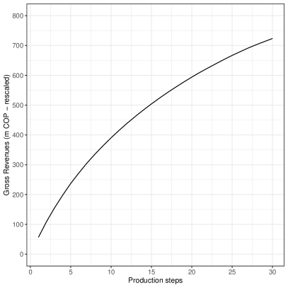
Figure A2: Concavity of the expected gross revenue function

Notes: Average gross revenues for EPMG.

Appendix B Inflow Forecasts

First, we run the following ARDL model using the weekly inflows of each generator $j$ as dependent variable,

$$\delta_{j,t}=\mu_{0}+\sum_{1\leq p\leq t}\alpha_{p}\delta_{j,t-p}+\sum_{1\leq q\leq t}\mathbf{\beta}_{q}\mathbf{x}_{j,t-q}+\epsilon_{j,t}\,\,\forall j$$ (B1)

We denote by $\delta_{j,t}$ the inflow to the focal dam in week $t$. $\mathbf{x}_{j,t}$ is a vector that includes the average maximum temperature and rainfalls in the past week at dam $j$, and information about the future probabilities of el niño. We average the data at the weekly level to reduce the extent of autocorrelation in the error term. Importantly for forecasting, the model does not include the contemporaneous effect of the explanatory variables.

Forecasting. For forecasting, we first determine the optimal number of lags for $P$ and $Q$ for each dam $j$ using the BIC criterion. Given the potential space of these two variables, we set $Q=P$ in (B1) to reduce the computation burden. For an h-ahead week forecast, we then run the following regression:

$$\delta_{j,t+h}=\hat{{\mu}}_{0}+\hat{\alpha}_{1}\delta_{t}+\cdots+\hat{\alpha}_{P}\delta_{j,t-P+1}+\sum_{k=1}^{K}\hat{\beta}_{1,k}x_{j,t,k}+\cdots+\hat{\beta}_{q,k}x_{j,t-Q+1,k}+\epsilon_{t},$$ (B2)

where $K$ denotes the number of control variables in $\textbf{x}_{j,t-q}$.

Forecasting algorithm. For each week $t$ of time series of dam $j$, we estimate (B2) for $h\in\{4,8,12,16,20\}$ weeks ahead (i.e., for each month up to five months ahead) using only data for the 104 weeks (2 years) before week $t$. In the analysis, we only keep dams for which we have at least 2 years of data to perform the forecast. Dropping this requirement does not affect the results.

Quality of the fit. Figures B1 and B2 report the autocorrelation function and the Ljung-box test for the error term $\epsilon_{t}$ in (B2) for the largest dams in Colombia in the period we consider. The p-values of Ljung-box test never reject the null of autocorrelation.

Analysis at the firm level. In the structural model, we estimate a transition matrix by using an ARLD model similar to that in (B1), with the only difference that the explanatory variables are averaged over months rather than weeks to better capture heterogeneity across seasons. We also control for early dummies to better account for long-term time variation like el niño. We present the autocorrelation function and Ljung-box tests in Appendix Figures B3 and B4. For estimation, we model the error term $\epsilon_{j,t}$ in (B1) through a Pearson Type IV distribution as commonly done in the hydrology literature. This distribution feats our purposes because it is not symmetric, meaning different probabilities at the tails (dry vs wet seasons). We show that this distribution fits well the data for the largest four diversified firms (ENDG, EPMG, EPSG, and ISGG) in Figures 3(a), 3(b), 3(c), and 3(d).

Figure B1: ARDL model diagnostics for some of the largest dams in Colombia in our sample period

(a) Guatape

(b) Pagua

(c) Guavio

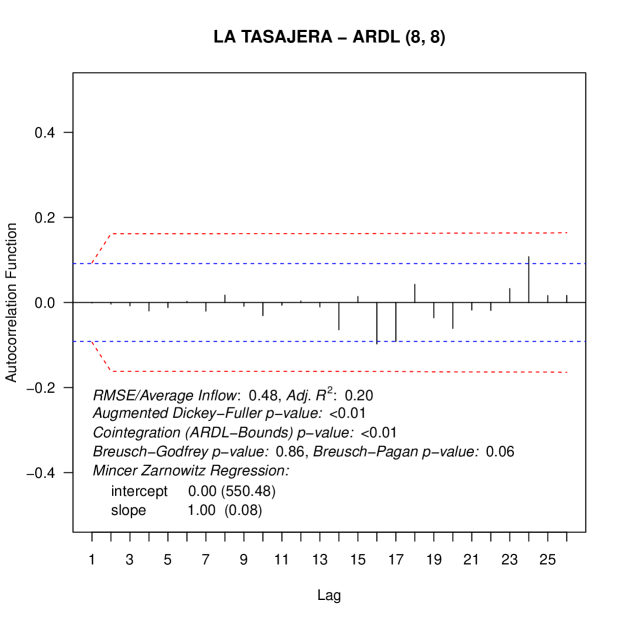
(d) La Tasajera

Notes: The plot shows the autocorrelation plots for the residuals of the ARDL model used to forecast future inflows. The title indicates the number of lagged dependent variables and explanatory variables selected by the algorithm. The test indicates the extent of autocorrelation and heteroskedasticity in the error terms.

Figure B2: Ljung boxes for some of the largest dams in Colombia

(a) Guatape

(b) Pagua

(c) Guavio

(d) La Tasajera

Notes: The plot shows the p-values of Ljung-box tests of whether any of a group of autocorrelations of a time series are different from zero.

Figure B3: ARDL model diagnostics at firm level

(a) ENDG

(b) EPMG

(c) EPSG

(d) ISGG

Notes: The plot shows the autocorrelation plots for the residuals of the ARDL model used to forecast future inflows at the firm level. The title indicates the number of lagged dependent variables and explanatory variables selected by the algorithm. The test indicates the extent of autocorrelation and heteroskedasticity in the error terms.

Figure B4: Ljung boxes at the firm level

(a) ENDG

(b) Pagua

(c) EPSG

(d) ISGG

Notes: The plot shows the p-values of Ljung-box tests of whether any of a group of autocorrelations of a time series are different from zero.

Figure B5: Transition matrix for ENDG

Note: The plots show the quality of the fit of the normal, logistic, and Pearson Type IV distribution to the error term from the ARDL model.

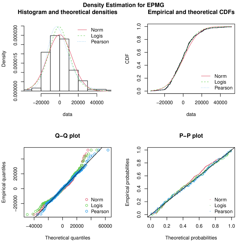
Figure B6: Transition matrix for EPMG

Note: The plots show the quality of the fit of the normal, logistic, and Pearson Type IV distribution to the error term from the ARDL model.

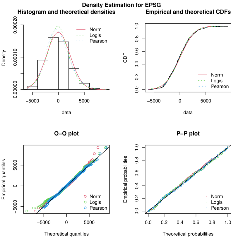
Figure B7: Transition matrix for EPSG

Note: The plots show the quality of the fit of the normal, logistic, and Pearson Type IV distribution to the error term from the ARDL model.

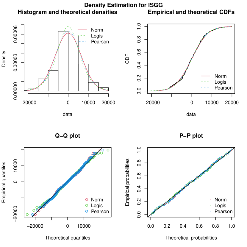
Figure B8: Transition matrix for ISGG

Note: The plots show the quality of the fit of the normal, logistic, and Pearson Type IV distribution to the error term from the ARDL model.

Appendix C Generators’ Responses to Inflow Forecasts

C.1 Symmetric Responses to Favorable and Adverse Forecasts

The main text focuses on generators’ responses to extreme forecasts. This section shows consistent results with a less flexible specification that forces firms to respond equally to favorable and adverse shocks. We employ the following specification:

$$y_{ij,th}=\sum^{L}_{l=1}\beta_{l}\,\widehat{inflow}_{ij,t+l}+\textbf{x}_{ij,t-1,h}\,\alpha+\mu_{j,m(t)}+\tau_{t}+\tau_{h}+\varepsilon_{ij,th},$$ (B3)

where the sole departure from (1) is that $\{\widehat{inflow}_{ij,t+l}\}_{l}$ is a vector of forecasted inflows $l$ months ahead. We also allow the slope of $j$’s lagged water stock to vary across generators to control for reservoir size across seasons to avoid the mechanical association between high forecast inflows and large reservoirs.

Zooming in on sibling thermal generators, we define $\{\widehat{inflow}_{ij,t+l}\}_{l}$ as the sum of the $l$-forecast inflows accruing to firm $i$, and by controlling for lagged total water stock by firms as in Section 3.2.2. In this case, we let the slope of this variable vary across firms.

C.1.1 The Response of Hydropower Generators

The top panel of Figure 1(f) plots the main coefficient of interest, $\beta_{l}$, for inflow forecasts one, three, and five months ahead. Panel (a) finds that dams are willing to produce approximately 5 % more per standard deviation increase in inflow forecast. The effect fades away for later forecasts. Generators respond mostly through quantity bids (black bars) rather than price bids (gray bars). To show that our predictions indeed capture variation that is material for firms, Panel (b) performs the same analysis as in (B3) using the forecast residuals (i.e., $inflow_{ij,t+l}-\widehat{inflow}_{ij,t+l}$), instead of the forecast. Reassuringly, we find that bids do not react to “unexpected inflows,” pointing to no additional information in the forecast residuals.

Figure C1: Symmetric hydropower generators’ responses to inflow forecasts

(a) Top Panel. All $l$-forecasts in the same regressions

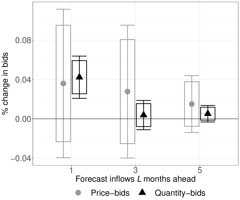
(b) Expected inflows (standardized forecasts)

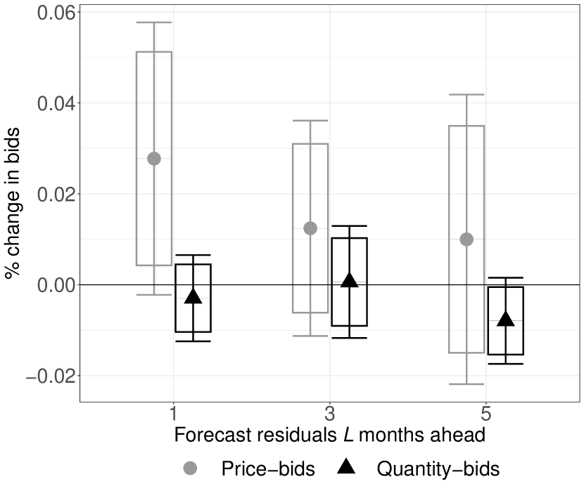
(c) Unexpected inflows (forecast residuals)

(d) Bottom Panel. Separate regressions for each month-ahead forecast

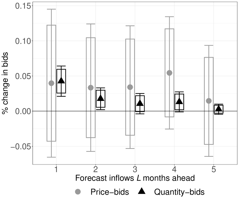
(e) Expected inflows (standardized forecasts)

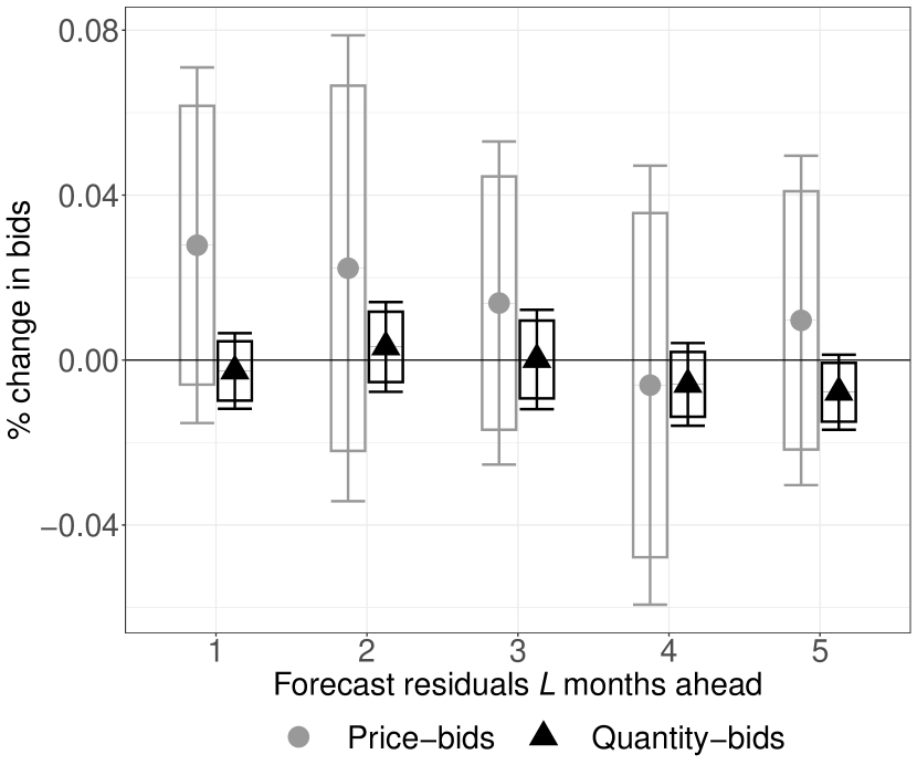
(f) Unexpected inflows (forecast residuals)

Notes: All plots report estimates of $\{\beta_{l}\}_{l}$ from (B3) for one, three, and five months ahead using either price- (gray) or quantity-bids as dependent variables. The bottom panels report coefficients for separate regressions (one for each month-ahead forecast). Left and right panels use the forecasted inflows or the forecast errors from the prediction exercise as independent variables, respectively. Error bars (boxes) report the 95% (90%) CI.

C.1.2 The Response of “Sibling” Thermal Generators

The coefficient estimates are in Figure C2. As in Section 3.2.2, sibling thermal generators respond mostly with their price-bids. The effect is particularly evident in Panel (b), which runs separate regressions for each monthly forecast in (B3) and shows that current thermal generators reflect inflow forecasts that are two to four months ahead.

Figure C2: Symmetric response of sibling thermal generators

(a) Single regression

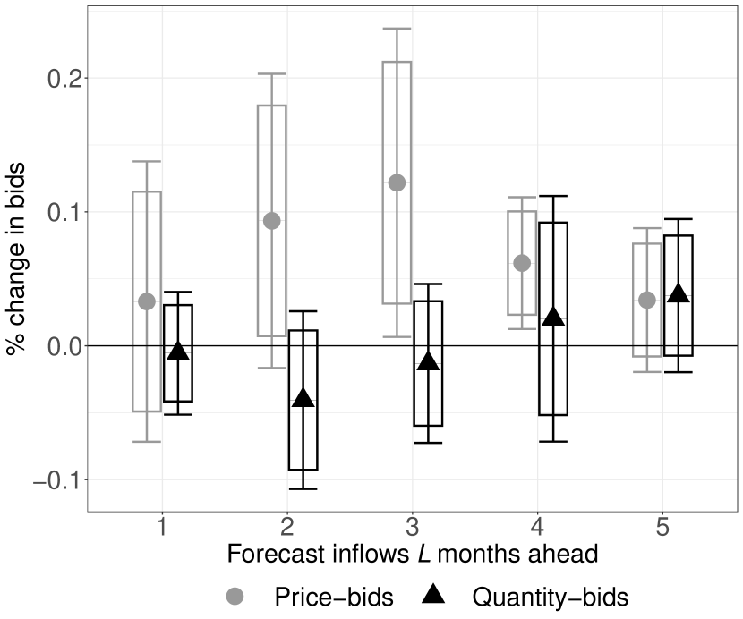
(b) Separate regressions

Notes: The figure reports estimates of $\{\beta_{l}\}_{l}$ from a modified version of (B3) where the focus is on water inflows accruing to a firm rather than to a generator between one and five months ahead. Since water inflow forecasts can be correlated over time, Panel (b) plots the estimates from five separate regressions with each regression focusing on a specific month. Error bars (boxes) report the 95% (90%) CI.

C.1.3 The Response to Competitors’ Inflow Forecasts

We include $\widehat{\text{infolow}}_{-i,t+l}$, the sum of the forecasted inflows of firm $i$’s competitors $l$ months ahead, in (B3) and estimate coefficients for both own-forecasts and competitors’ forecasts. Figure C3 shows the estimated coefficients for competitors’ and own’s forecasts in blue and green, respectively. Two results emerge. First, generators do not respond to competitors. We test and do not reject the joint hypothesis that the coefficients pertaining to the competitors are jointly equal to zero. Second, a dam’s responses to its own forecasts are quantitatively similar to those in Panel (a) of Figure 1(f), indicating little correlation between its own forecasts and competitors’ forecasts.

Figure C3: Generators’ response to competitors and own forecasts

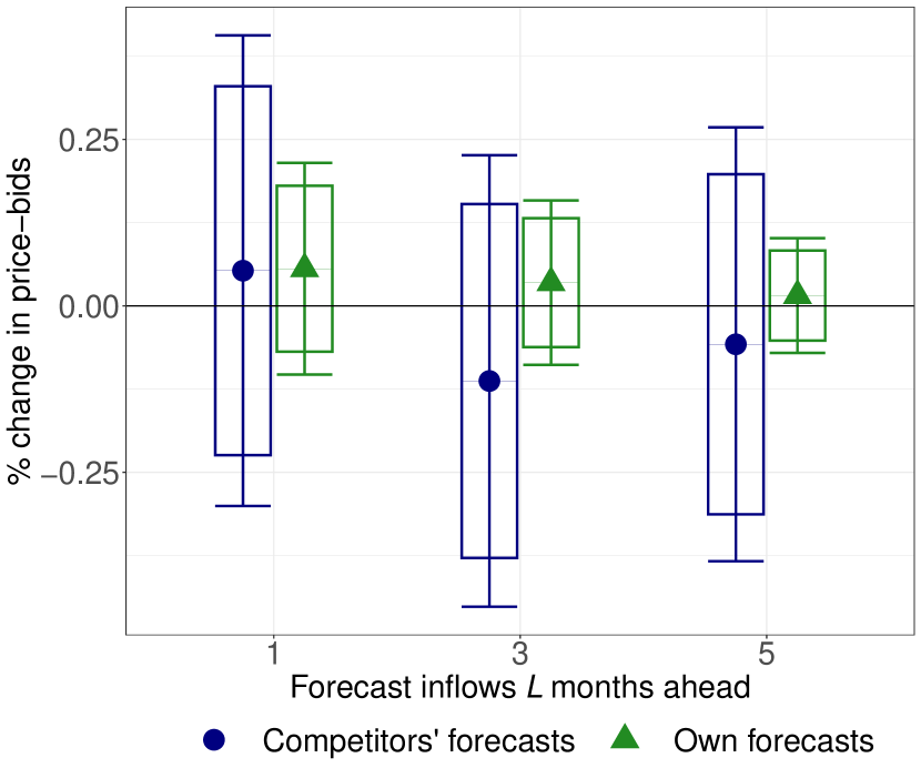
(a) Price bids

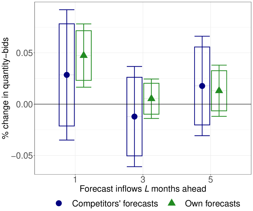
(b) Quantity bids

Notes: The figure reports the estimates from a modified version of (B3) where we include both a generator’s water forecasted inflow (green) and that of its competitors (blue). Joint test p-values for competitors’ forecasts are 0.6763 for price bids and 0.594 for quantity bids. Error bars (boxes) report the 95% (90%) CI. Error bars (boxes) report the 95% (90%) CI.

Current water stocks. Intrigued by the fact that generators do not respond to dry spells accruing to competitors, we extend our analysis to investigate firms’ responses to other firms. We propose a simple framework where we regress a firm’s hourly quantity- and price-bids (in logs) on a firm’s current water stock, the water stock of its competitors, and the interaction of these two variables. As before, we average variables across weeks. We account for unobserved heterogeneity at the level of a generator or the macro level (e.g., demand) using fixed effects by generators, week-by-year, and market hours. Table C2 finds that firms only respond to their own water stocks: not only the response to competitors is not statistically significant, but also its magnitude is shadowed by that observed for own water stocks. In addition, the interaction term is small and insignificant, indicating that firms do not strategize based on their potential competitive advantage.

Table C1: Firm response to competitors’ water stock, two-by-two matrices

	(1)		(2)		(3)		(4)		(5)		(6)		(7)		(8)
	Quantity-bids ($\ln$)								Price-bids ($\ln$)
Panel a. Controlling for a Competitors’ Water Stocks
Low water stock for $i$	–0.166				–0.160				0.004				0.004
	(0.101)				(0.092)				(0.085)				(0.086)
Low water stock for $i$’s comp.	–0.044		0.043						0.003		0.004
	(0.085)		(0.068)						(0.055)		(0.079)
High water stock for $i$			0.062	∗∗			0.048				–0.089				–0.077
			(0.021)				(0.028)				(0.061)				(0.068)
High water stock for $i$’s comp.					–0.096		–0.061						0.105		0.050
					(0.055)		(0.071)						(0.092)		(0.115)
$N$	135,048		135,048		135,048		135,048		135,048		135,048		135,048		135,048
Adjusted R-squared	0.7874		0.7850		0.7877		0.7850		0.6316		0.6323		0.6319		0.6324
Panel b. Responding to Competitors’ Water Stocks
Low water stock for $i$	–0.196		–0.167						–0.047		0.006
	(0.133)		(0.095)						(0.107)		(0.096)
Low water stock for $i$’s comp.	–0.069				0.042				–0.041				0.015
	(0.103)				(0.066)				(0.025)				(0.077)
Low water stock for $i$ $\times$ Low water stock for $i$’s comp.	0.090								0.155
	(0.114)								(0.122)
High water stock for $i$’s comp.			–0.102				–0.061				0.107				0.072
			(0.054)				(0.089)				(0.094)				(0.109)
Low water stock for $i$ $\times$ High water stock for $i$’s comp.			0.130								–0.048
			(0.092)								(0.195)
High water stock for $i$					0.060	∗	0.047						–0.073		–0.054
					(0.025)		(0.048)						(0.055)		(0.064)
High water stock for $i$ $\times$ Low water stock for $i$’s comp.					0.028								–0.249
					(0.051)								(0.235)
High water stock for $i$ $\times$ High water stock for $i$’s comp.							0.003								–0.066
							(0.077)								(0.044)
$N$	135,048		135,048		135,048		135,048		135,048		135,048		135,048		135,048
Adjusted R-squared	0.7876		0.7877		0.7850		0.7850		0.6321		0.6319		0.6327		0.6324
FE: Generator, week-by-year, and hour	$\checkmark$		$\checkmark$		$\checkmark$		$\checkmark$		$\checkmark$		$\checkmark$		$\checkmark$		$\checkmark$
Clustered s.e., generator, month, and year	$\checkmark$		$\checkmark$		$\checkmark$		$\checkmark$		$\checkmark$		$\checkmark$		$\checkmark$		$\checkmark$
* – $p<0.1$; ** – $p<0.05$; *** – $p<0.01$

• Notes: The top panel presents the coefficient estimates from the following regression

  $$\ln bid_{ijht}=\alpha_{0}+\beta_{i}\mathds{1}_{it}+\beta_{-i}\mathds{1}_{-it}+\beta_{2}\delta_{ijt}+FE_{jht}+\varepsilon_{ijht},$$

  where $t$ indices weeks, so that price- and quantity-bids are averaged across weeks for each hour. The definition of $\mathds{1}_{it}$ varies across “Low water stocks,” when it takes the value of one if the sum of the water stocks of firm $i$ in week $t$ is below its 20^th percentile, or “High water stocks,” when the sum is above its 80^th percentile. $\mathds{1}_{-it}$ is defined analogously for firm $i$’s competitors. Panel b also includes $\mathds{1}_{it}\cdot\mathds{1}_{-it}$ as a regressor, namely the interaction between a firm’s current status (whether $i$’s water stock is above or below a certain threshold and that of its average competitor). All regression control for a generator’s current inflow ($\delta_{ijt}$, unreported), and generator, week-by-year, and hour-fixed effects.

Table C2: Firm response to competitors’ water stock

	(1)		(2)		(3)		(4)		(5)		(6)
	Quantity-bids ($\ln$)						Price-bids ($\ln$)
Ln competitors’ water stock (std)	–0.106	∗	0.169		0.225		0.250		0.368		0.522
	(0.042)		(0.087)		(0.126)		(0.194)		(0.275)		(0.312)
Ln firm $i$’s water stock (std)			0.537	∗∗	0.584	∗∗			0.231		0.359	∗
			(0.179)		(0.191)				(0.185)		(0.148)
Ln competitors’ water stock (std) $\times$ Ln firm $i$’s water stock (std)					–0.029						–0.079
					(0.030)						(0.061)
Constant	5.778	∗∗∗	5.778	∗∗∗	5.762	∗∗∗	11.716	∗∗∗	11.716	∗∗∗	11.670	∗∗∗
	(0.001)		(0.009)		(0.016)		(0.000)		(0.008)		(0.038)
FE: Generator, week-by-year, and hour	$\checkmark$		$\checkmark$		$\checkmark$		$\checkmark$		$\checkmark$		$\checkmark$
Clustered s.e. by generator, month, and year	$\checkmark$		$\checkmark$		$\checkmark$		$\checkmark$		$\checkmark$		$\checkmark$
$N$	135,048		135,048		135,048		135,048		135,048		135,048
Adjusted R-squared	0.7776		0.7856		0.7858		0.6246		0.6259		0.6277
* – $p<0.1$; ** – $p<0.05$; *** – $p<0.01$

• Notes: This table presents the coefficient estimates from the following regression

  $$\ln bid_{ijht}=\alpha_{0}+\beta_{i}\ln w_{it}+\beta_{-i}\ln w_{-it}+\beta_{int}\ln w_{it}\cdot\ln w_{-it}+FE_{jht}+\varepsilon_{ijht},$$

  where $t$ indices weeks, so that price- and quantity-bids are averaged across weeks for each hour. $w_{it}$ and $w_{-it}$ are the average weekly water stocks of firm $i$ and firm $i$’s competitors in week $t$. Continuous variables are standardized.

C.2 Robustness

Figure C4: Hydropower generators’ responses to inflow forecasts over 1, 2, and 3 months

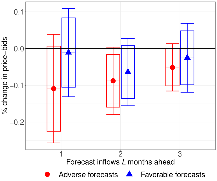
(a) Price bids

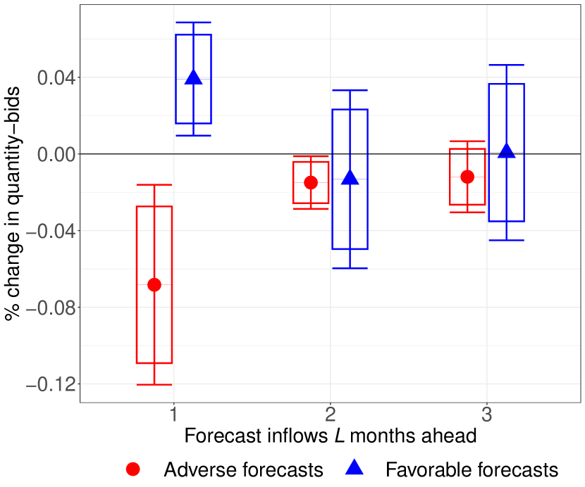
(b) Quantity bids

Notes: The figure studies how hydropower generators respond to favorable or adverse future water forecasts according to (1). Each plot reports estimates of $\{\beta^{low}_{l}\}$ in red and $\{\beta^{high}_{l}\}$ in blue for one, three, and five months ahead. Error bars (boxes) report the 95% (90%) CI.

Figure C5: Hydropower generators’ responses to inflow forecasts - separate regressions

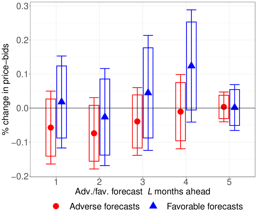
(a) Price bids

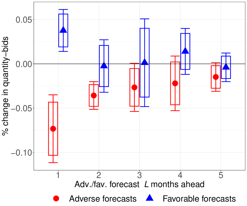
(b) Quantity bids

Notes: The figure studies how hydropower generators respond to favorable or adverse future water forecasts by running (1) five times – i.e., in each regression, we keep only one pair of adverse and favorable variable for each one of the five monthly forecasts reported in the figure. Each plot reports estimates of $\{\beta^{low}_{l}\}$ in red and $\{\beta^{high}_{l}\}$ in blue for one, three, and five months ahead. Error bars (boxes) report the 95% (90%) CI.

Figure C6: Sibling thermal generators’ responses over 1, 2, and 3 months

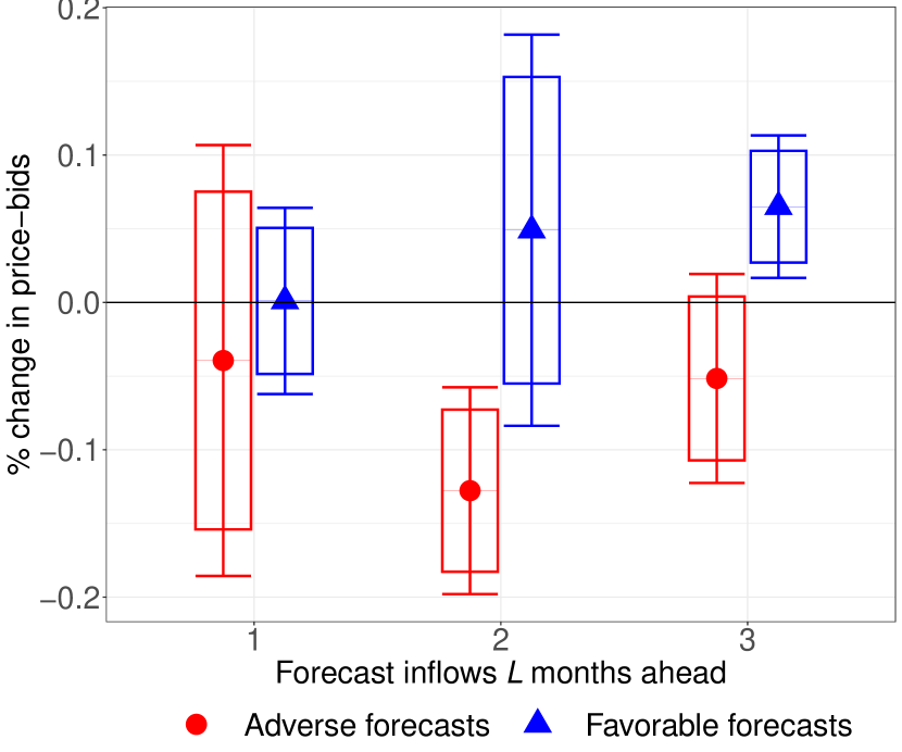
(a) Price bids

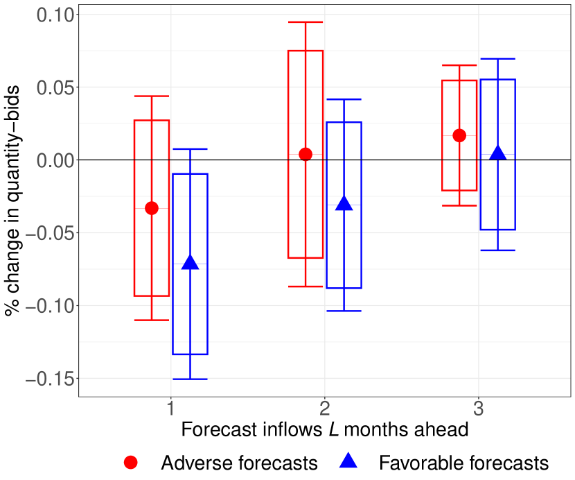
(b) Quantity bids

Notes: The figure studies how sibling thermal generators respond to favorable or adverse future water forecasts according to (1). Each plot reports estimates of $\{\beta^{low}_{l}\}$ in red and $\{\beta^{high}_{l}\}$ in blue for one, three, and five months ahead. Error bars (boxes) report the 95% (90%) CI.

Figure C7: Hydro generator’s responses to competitors’ forecasts over 1, 2, and 3 months

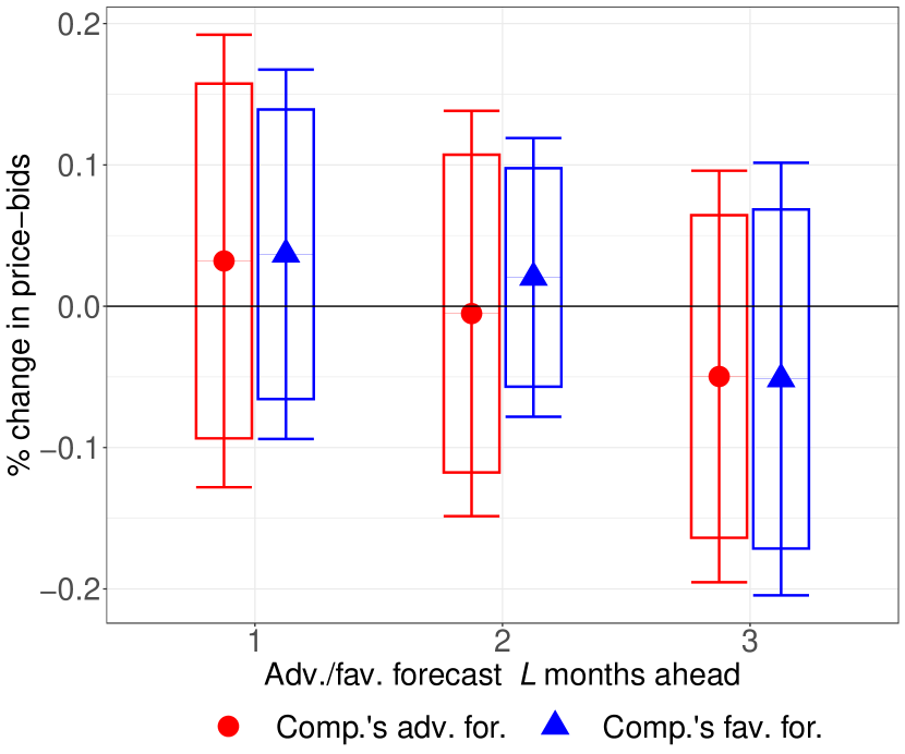
(a) Price bids

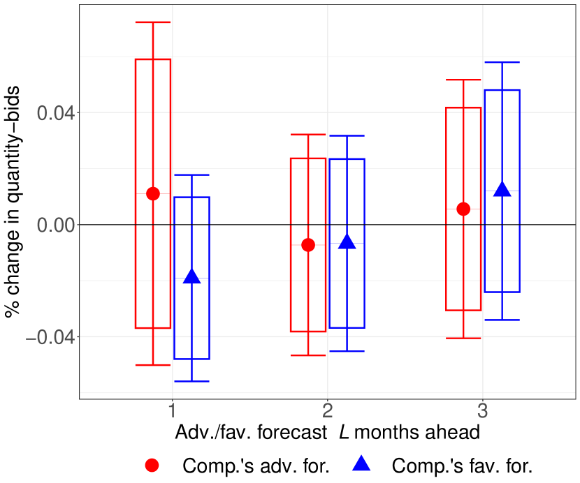
(b) Quantity bids

Notes: The figure studies how generators respond to favorable or adverse future water forecasts accruing to competitors according to (1). Error bars (boxes) report the 95% (90%) CI. Joint tests for $\{\beta^{low}_{l}\}_{l=1}^{3}$ and $\{\beta^{high}_{l}\}_{l=1}^{3}$ reject the null hypothesis that these coefficients are zero.

Appendix D Exhibits from the Structural Model

Figure D1: Relationship between prices and business stealing

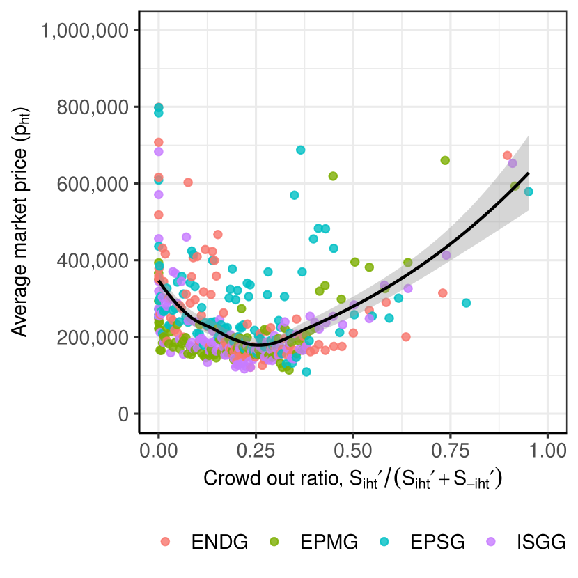
(a) Scarcity periods

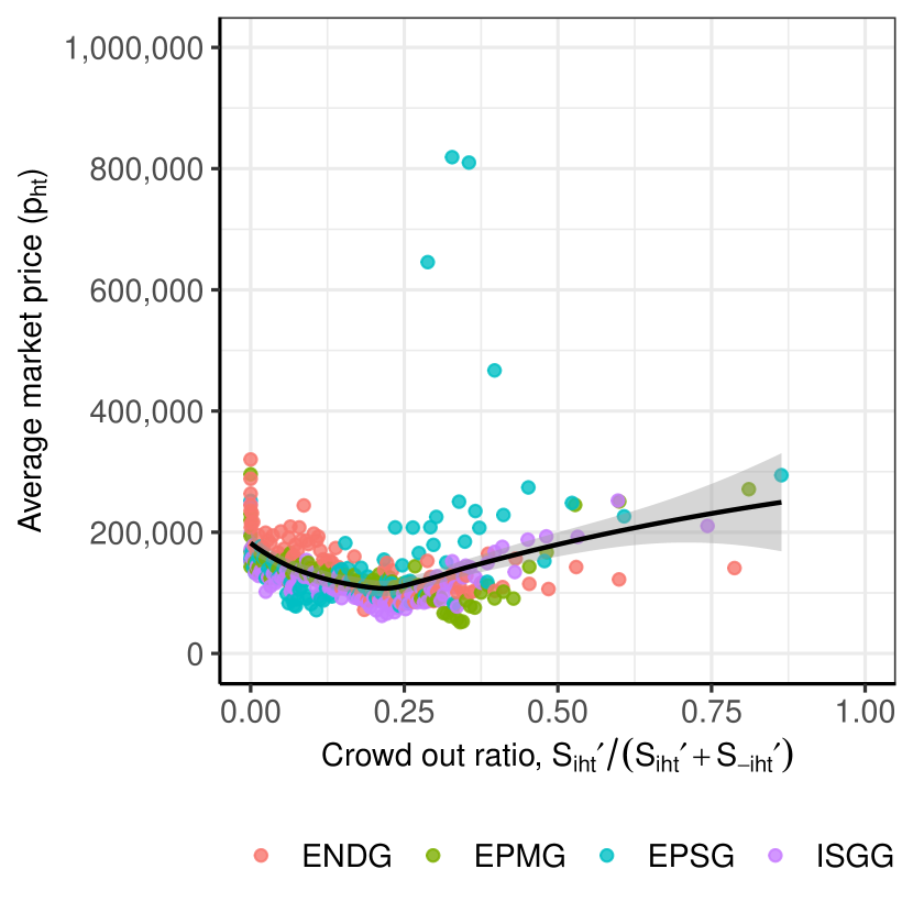
(b) Abundant periods

Notes: The figure presents binned scatter plots (100 bins per firm) of the market prices ($y$-axis) for different levels of business stealing ($x$-axis). To avoid dividing by zero when ${D^{R}_{i}}^{\prime}=0$, we let the x-axis be ${S_{iht}^{\prime}(p)}/({S_{iht}^{\prime}(p)}+{S_{-iht}^{\prime}(p)})$. The denominator is the sum of ${S_{iht}^{\prime}(p)}+{S_{-iht}^{\prime}(p)}$ instead of just $S_{-iht}^{\prime}(p)={D^{R}_{iht}}^{\prime}(p)$ as in (5) to account for ${D^{R}_{iht}}^{\prime}(p)\simeq 0$ without truncating the data. Only diversified firms with a dam are considered. The black line fits the data through a spline (the 95% CI is in gray). Panel (a) focuses on markets where firm $i$ has less than the 30^th percentile of its long-run water stock. Panel (b) focuses on periods where it has more than the 70^th percentile.

Table D1: Estimated primitives – four spline parameters

(1) (2) (3) (4) Marginal costs (COP/MWh) Thermal $(\psi^{thermal})$ 204460.10 ^∗∗∗ 151965.08 ^∗∗∗ 213177.19 ^∗∗∗ 149699.10 ^∗∗∗ (1,880.65) (1,840.22) (1,626.95) (1,624.97) Hydropower $(\psi^{hydro})$ 76,022.12 ^∗∗∗ 28,820.29 ^∗∗∗ 44,941.37 ^∗∗∗ 51,297.15 ^∗∗∗ (6,601.03) (6,290.74) (3,368.43) (4,638.29) Intertemporal value of water (COP/MWh) Spline 1 $(\gamma_{1})$ –2,216.01 ^∗∗∗ 6,992.47 ^∗∗∗ 2,297.60 ^∗∗∗ 10,797.46 ^∗∗∗ (710.63) (524.16) (372.92) (474.35) Spline 2 $(\gamma_{2})$ –2.773e-03 ^∗∗∗ –2.668e-03 ^∗∗∗ –3.672e-03 ^∗∗∗ –3.576e-03 ^∗∗∗ (2.612e-04) (1.550e-04) (1.398e-04) (1.402e-04) Spline 3 $(\gamma_{3})$ 5.359e-09 ^∗∗∗ 1.386e-08 ^∗∗∗ 5.512e-09 ^∗∗∗ 1.382e-08 ^∗∗∗ (6.862e-10) (6.043e-10) (4.654e-10) (5.307e-10) Spline 4 $(\gamma_{4})$ 2.364e-08 ^∗∗∗ –1.893e-08 ^∗∗∗ 1.220e-08 ^∗∗∗ –1.996e-08 ^∗∗∗ (2.347e-09) (1.773e-09) (1.382e-09) (1.536e-09) Fixed Effects Firm $\checkmark$ $\checkmark$ $\checkmark$ $\checkmark$ Generator $\checkmark$ Month-by-technology $\checkmark$ $\checkmark$ Hour $\checkmark$ $\checkmark$ $\checkmark$ $\checkmark$ Week-by-year $\checkmark$ $\checkmark$ Date $\checkmark$ $\checkmark$ Clustered s.e. Generator Generator Generator Generator SW F $(\psi^{thermal})$ 32.93 842.34 30.56 129.27 SW F $(\psi^{thermal})$ 2,314.39 760.89 3,458.28 700.41 SW F $(\psi^{hydro})$ 425.23 245.77 866.70 333.94 SW F $(\gamma_{1})$ 318.26 242.54 392.31 269.99 SW F $(\gamma_{2})$ 244.94 275.53 366.43 323.50 SW F $(\gamma_{3})$ 623.17 484.66 519.66 491.27 SW F $(\gamma_{4})$ 394.17 448.36 445.26 446.16 Anderson Rubin F 1,213.31 1,395.05 1,527.77 1,539.08 N 1,451,592 1,451,592 1,451,592 1,451,592 * – $p<0.1$; ** – $p<0.05$; *** – $p<0.01$

• Notes: This table presents the coefficients obtained estimating (12) by two-stage least squares on daily data between January 1, 2010, and December 31, 2015. Unlike the results presented in the main text (Table 2), these estimates are based on an approximation of the value function over four knots instead of five, meaning that we estimate only four $\{\gamma\}_{r=1}^{4}$. The top panels separate the marginal cost estimates and the value function parameters from the fixed effects used in estimation, which vary across columns. Our favorite specification is in Column (4), which includes day-fixed effects. The bottom panel provides diagnostic tests in the first stage. 2,900 COP $\simeq$ 1 US$

Table D2: Estimated primitives – employing a normal density for the transition matrix

(1) (2) (3) (4) Marginal costs (COP/MWh) Thermal $(\psi^{thermal})$ 204727.14 ^∗∗∗ 143319.87 ^∗∗∗ 220441.60 ^∗∗∗ 146635.86 ^∗∗∗ (1,803.36) (1,843.71) (1,644.41) (1,529.32) Hydropower $(\psi^{hydro})$ 46,491.28 ^∗∗∗ 28,163.59 ^∗∗∗ 28,458.10 ^∗∗∗ 60,353.00 ^∗∗∗ (7,097.17) (5,026.09) (3,774.68) (3,616.79) Intertemporal value of water (COP/MWh) Spline 1 $(\gamma_{1})$ –797.45 –6,751.10 ^∗∗∗ –9,712.11 ^∗∗∗ –3,744.90 ^∗∗∗ (1,018.26) (504.77) (526.92) (364.28) Spline 2 $(\gamma_{2})$ –3.346e-03 ^∗∗∗ –3.154e-04 ^∗∗ –2.173e-04 –1.064e-03 ^∗∗∗ (3.548e-04) (1.421e-04) (1.806e-04) (1.016e-04) Spline 3 $(\gamma_{3})$ –4.894e-09 ^∗∗∗ 2.009e-08 ^∗∗∗ –1.621e-08 ^∗∗∗ 1.837e-08 ^∗∗∗ (1.497e-09) (1.055e-09) (1.093e-09) (8.171e-10) Spline 4 $(\gamma_{4})$ 4.070e-08 ^∗∗∗ –3.179e-08 ^∗∗∗ 4.205e-08 ^∗∗∗ –2.848e-08 ^∗∗∗ (2.795e-09) (1.931e-09) (1.926e-09) (1.508e-09) Spline 5 $(\gamma_{5})$ –2.216e-08 ^∗∗∗ 8.949e-08 ^∗∗∗ 4.422e-08 ^∗∗∗ 8.251e-08 ^∗∗∗ (3.405e-09) (2.893e-09) (2.274e-09) (2.500e-09) Fixed Effects Firm $\checkmark$ $\checkmark$ $\checkmark$ $\checkmark$ Generator $\checkmark$ $\checkmark$ $\checkmark$ $\checkmark$ Month-by-technology $\checkmark$ $\checkmark$ Hour $\checkmark$ $\checkmark$ $\checkmark$ $\checkmark$ Week-by-year $\checkmark$ $\checkmark$ FE: Date $\checkmark$ $\checkmark$ SW F $(\psi^{thermal})$ 3,129.14 1,257.31 2,991.60 1,097.29 SW F $(\psi^{hydro})$ 443.62 272.74 883.91 367.55 SW F $(\psi^{\gamma_{1}})$ 251.73 213.67 285.62 225.96 SW F $(\psi^{\gamma_{2}})$ 219.64 273.32 270.25 300.83 SW F $(\psi^{\gamma_{3}})$ 441.27 476.05 297.84 482.88 SW F $(\psi^{\gamma_{4}})$ 522.38 550.59 296.71 553.52 SW F $(\psi^{\gamma_{5}})$ 403.80 1,255.92 485.36 1,018.15 Anderson Rubin F 1,213.31 1,395.05 1,527.77 1,539.08 KP Wald 156.38 156.56 139.15 159.40 N 1,451,592 1,451,592 1,451,592 1,451,592 * – $p<0.1$; ** – $p<0.05$; *** – $p<0.01$

• Notes: This table presents the coefficients obtained estimating (12) by two-stage least squares on daily data between January 1, 2010, and December 31, 2015. Unlike the results presented in the main text (Table 2), these estimates assume that the transition matrix is normally distributed. The top panels separate the marginal cost estimates and the value function parameters from the fixed effects used in estimation, which vary across columns. Our favorite specification is in Column (4), which includes day-fixed effects. The bottom panel provides diagnostic tests in the first stage. 2,900 COP $\simeq$ 1 US$

Table D3: Estimated primitives – employing a normal density for the transition matrix

(1) (2) (3) (4) Marginal costs (COP/MWh) Thermal $(\psi^{thermal})$ 195271.35 ^∗∗∗ 152621.02 ^∗∗∗ 194831.41 ^∗∗∗ 151112.79 ^∗∗∗ (1,605.71) (1,807.59) (1,229.58) (1,573.39) Hydropower $(\psi^{hydro})$ 120408.48 ^∗∗∗ 32,919.28 ^∗∗∗ 128840.47 ^∗∗∗ 59,085.78 ^∗∗∗ (1,313.47) (5,997.03) (871.55) (4,459.66) Intertemporal value of water (COP/MWh) Spline 1 $(\gamma_{1})$ –2,720.98 ^∗∗∗ 6,297.20 ^∗∗∗ 1,569.04 ^∗∗∗ 10,291.14 ^∗∗∗ (635.73) (515.56) (329.00) (461.14) Spline 2 $(\gamma_{2})$ –2.752e-03 ^∗∗∗ –2.829e-03 ^∗∗∗ –3.485e-03 ^∗∗∗ –3.836e-03 ^∗∗∗ (2.242e-04) (1.588e-04) (1.235e-04) (1.425e-04) Spline 3 $(\gamma_{3})$ 7.278e-09 ^∗∗∗ 1.527e-08 ^∗∗∗ 1.025e-08 ^∗∗∗ 1.538e-08 ^∗∗∗ (7.491e-10) (6.213e-10) (4.369e-10) (5.414e-10) Spline 4 $(\gamma_{4})$ 1.844e-08 ^∗∗∗ –2.010e-08 ^∗∗∗ –4.491e-09 ^∗∗∗ –2.165e-08 ^∗∗∗ (2.351e-09) (1.804e-09) (1.222e-09) (1.550e-09) Fixed Effects FE: Firm $\checkmark$ $\checkmark$ $\checkmark$ $\checkmark$ FE: Generator $\checkmark$ $\checkmark$ FE: Month-by-technology $\checkmark$ $\checkmark$ FE: Hour $\checkmark$ $\checkmark$ $\checkmark$ $\checkmark$ FE: Week-by-year $\checkmark$ $\checkmark$ FE: Date $\checkmark$ $\checkmark$ Clustered s.e. Generator Generator Generator Generator SW F $(\psi^{thermal})$ 36.41 113.62 34.13 94.59 SW F $(\psi^{hydro})$ 124.43 300.57 139.18 2,474.37 SW F $({\gamma_{1}})$ 616.23 652.90 483.22 617.59 SW F $({\gamma_{2}})$ 1,401.71 364.00 194.38 284.03 SW F $({\gamma_{3}})$ 76.56 93.11 644.24 248.55 SW F $({\gamma_{4}})$ 45.66 86.99 1,139.58 82.71 Anderson Rubin F 19.74 111.61 196.42 106.90 KP Wald 7.16 10.80 6.61 19.28 Overid. p-value 0.19 0.21 0.11 0.14 N 1,451,592 1,451,592 1,451,592 1,451,592 * – $p<0.1$; ** – $p<0.05$; *** – $p<0.01$

• Notes: This table presents the coefficients obtained estimating (12) by two-stage least squares on daily data between January 1, 2010, and December 31, 2015. Unlike the results presented in the main text (Table 2), these estimates assume that the transition matrix is normally distributed and are based on an approximation of the value function over four knots instead of five, meaning that we estimate only four $\{\gamma\}_{r=1}^{4}$. The top panels separate the marginal cost estimates and the value function parameters from the fixed effects used in estimation, which vary across columns. Our favorite specification is in Column (4), which includes day-fixed effects. The bottom panel provides diagnostic tests in the first stage. 2,900 COP $\simeq$ 1 US$

Appendix E Smoothing Variables

This section details the smoothing approach that allows interchanging differentiation and expectation after taking the first-order conditions of the value function (9) – that is, $\frac{\partial\int_{\epsilon}V(w,p(\epsilon))f_{\epsilon}(\epsilon)\text{d}\epsilon}{\partial p}=\int_{\epsilon}\frac{\partial V(w,p(\epsilon))}{\partial p}f_{\epsilon}(\epsilon)\text{d}\epsilon$ – simplifying the interpretation and identification in Section 5. The smoothing procedure replaces indicators in supply and demand variables with their smoothed version.

Residual demand of firm $i$. Following the notation in Section 5, the residual demand to firm $i$ is $\tilde{D}^{R}_{iht}(p,\epsilon)=D_{ht}(\epsilon)-\tilde{S}_{-iht}(p)$, where the notation $\tilde{x}$ means that variable $x$ is smoothed. Smoothing the residual demand follows from smoothing the supply of the competitors of firm $i$, $\tilde{S}_{-iht}(p)=\sum_{m\neq i}^{N}\sum_{j=1}^{J_{m}}q_{mjht}\mathcal{K}\Big{(}\frac{p-b_{mjt}}{bw}\Big{)}$, where $J_{m}$ is the number of generation units owned by firm $m$. Let $\mathcal{K}(\cdot)$ denote the smoothing kernel, which we choose to be the standard normal distribution in the estimation wolak2007quantifying. We follow ryan2021competitive and set $bw$ equal to 10% of the expected price in MWh. The derivative of $D^{R}_{iht}(p,\epsilon)$ with respect to the market price in hour $h$ and day $t$ is

$$\frac{\partial\tilde{D}^{R}_{iht}(p,\epsilon)}{\partial p_{ht}}=-\sum_{m\neq i}^{N}\sum_{k=1}^{K_{m}}q_{mkht}\frac{\partial\mathcal{K}\big{(}\frac{p-b_{mkt}}{bw}\big{)}}{\partial p_{ht}}.$$

Supply of firm $i$. The supply of firm $i$ becomes, $\tilde{S}_{iht}(p_{ht})=\sum_{j=1}^{J_{i}}q_{ijht}\mathcal{K}\Big{(}\frac{p-b_{ijt}}{bw}\Big{)}$, leading to the following smoothed derivatives,

$$\frac{\partial\tilde{S}_{iht}}{\partial p_{ht}}=\sum_{j=1}^{J_{i}}q_{ijht}\frac{\partial\mathcal{K}\big{(}\frac{p-b_{mkt}}{bw}\big{)}}{\partial p_{ht}},\hskip 8.61108pt\frac{\partial\tilde{S}_{iht}}{\partial q_{ijht}}=\mathcal{K}\Big{(}\frac{p-b_{ijt}}{bw}\Big{)},\hskip 4.30554pt\frac{\partial\tilde{S}_{iht}}{\partial b_{ijt}}=-q_{ijht}\frac{\partial\mathcal{K}\big{(}\frac{p-b_{ijt}}{bw}\big{)}}{\partial b_{ijt}}.$$

The derivatives of the smoothed supply functions by technology $\tau$ are found analogously:

$$\frac{\partial\tilde{S}_{iht}^{\tau}}{\partial p_{ht}} =\sum_{k\in\tau}q_{ikht}\frac{\partial\mathcal{K}\big{(}\frac{p-b_{ikt}}{bw}\big{)}}{\partial p_{ht}},$$

$$\frac{\partial\tilde{S}_{iht}^{\tau}}{\partial q_{ijht}} =\begin{cases}\mathcal{K}\Big{(}\frac{p-b_{ijt}}{bw}\Big{)}&\textnormal{ if $j$ has technology }\tau,\\ 0&\textnormal{ otherwise, }\end{cases}$$

$$\frac{\partial\tilde{S}_{iht}^{\tau}}{\partial b_{ijt}} =\begin{cases}-q_{ijht}\frac{\partial\mathcal{K}\big{(}\frac{p-b_{ijt}}{bw}\big{)}}{\partial b_{ijt}}&\textnormal{ if $j$ has technology }\tau,\\ 0&\textnormal{ otherwise. }\end{cases}$$

Market price. The derivatives of the market price with respect to price- and quantity-bids in (9) are computed using the envelop theorem. Their smoothed versions are

$$\frac{\partial p_{ht}}{\partial b_{ijt}}=\frac{\frac{\partial\tilde{S}_{iht}}{\partial b_{ijt}}}{\frac{\partial\tilde{D}^{R}_{iht}}{\partial p_{ht}}-\frac{\partial\tilde{S}_{iht}}{\partial p_{ht}}},\hskip 85.35826pt\frac{\partial p_{ht}}{\partial q_{ijht}}=\frac{\frac{\partial\tilde{S}_{iht}}{\partial q_{ijht}}}{\frac{\partial\tilde{D}^{R}_{iht}}{\partial p_{ht}}-\frac{\partial\tilde{S}_{iht}}{\partial p_{ht}}}.$$

Appendix F Model Fit

Table F1: Hourly prices across simulations

	(1)	(2)	(3)	(4)		(5)	(6)	(7)	(8)
Hour	Avg.Prices	Avg.Sim Prices	Avg.Price Dif	Avg.Price Dif	Hour	Avg. Prices	Avg.Sim Prices	Avg.Price Dif	Avg.Price Dif
	Cop MWh	Cop MWh	Cop MWh	Cop MWh%		Cop MWh	Cop MWh	Cop MWh	Cop MWh%
10 steps for all variables
0	161,252.60	135,273.40	-25,979.24	-6.26	12	195,531.40	163,482.30	-32,049.12	-11.77
1	156,664.90	130,628.70	-26,036.24	-6.95	13	194,709.30	163,511.20	-31,198.11	-11.86
2	152,892.30	128,465.70	-24,426.53	-6.08	14	196,454.30	164,380.80	-32,073.58	-12.15
3	151,443.70	128,594.40	-22,849.36	-6.03	15	194,546.70	162,841.40	-31,705.25	-12.01
4	154,896.60	129,640.90	-25,255.72	-7.31	16	191,133.60	160,444.40	-30,689.27	-11.30
5	163,513.80	135,057.40	-28,456.36	-8.86	17	189,147.60	159,043.90	-30,103.68	-10.45
6	165,598.20	136,721.60	-28,876.58	-9.43	18	211,991.70	177,970.30	-34,021.39	-13.46
7	174,317.70	142,618.10	-31,699.63	-10.85	19	225,075.80	185,115.50	-39,960.33	-15.82
8	183,744.00	151,396.80	-32,347.23	-11.71	20	207,064.00	173,728.10	-33,335.85	-12.43
9	188,755.90	155,528.70	-33,227.22	-12.04	21	194,239.10	162,719.60	-31,519.55	-11.23
10	194,980.90	162,327.90	-32,652.96	-12.38	22	181,601.30	151,125.00	-30,476.31	-9.83
11	200,586.40	166,731.60	-33,854.77	-13.54	23	170,168.10	139,515.30	-30,652.76	-10.08
30 steps for residual demand and value function, 10 steps for supply schedules
0	161,252.60	138,807.00	-22,445.62	-5.30	12	195,531.40	164,607.50	-30,923.88	-9.30
1	156,664.90	133,723.50	-22,941.38	-5.33	13	194,709.30	164,046.20	-30,663.15	-9.26
2	152,892.30	132,266.60	-20,625.70	-3.92	14	196,454.30	165,683.90	-30,770.43	-9.46
3	151,443.70	132,024.60	-19,419.11	-4.10	15	194,546.70	163,824.30	-30,722.39	-9.47
4	154,896.60	133,081.20	-21,815.40	-5.82	16	191,133.60	161,973.50	-29,160.14	-9.27
5	163,513.80	138,363.60	-25,150.15	-7.21	17	189,147.60	160,533.10	-28,614.54	-8.59
6	165,598.20	141,354.20	-24,243.99	-7.42	18	211,991.70	180,689.50	-31,302.22	-11.04
7	174,317.70	147,567.70	-26,750.04	-8.10	19	225,075.80	187,535.60	-37,540.19	-14.00
8	183,744.00	153,035.40	-30,708.67	-10.45	20	207,064.00	175,701.60	-31,362.38	-10.01
9	188,755.90	157,682.30	-31,073.58	-9.70	21	194,239.10	162,380.70	-31,858.44	-10.22
10	194,980.90	163,022.50	-31,958.37	-10.36	22	181,601.30	152,607.30	-28,993.96	-7.55
11	200,586.40	167,918.50	-32,667.87	-11.56	23	170,168.10	144,076.90	-26,091.15	-7.36

• Notes: The table compares average hourly prices across the simulated and actual data. The simulation model is described in Section 6.2. The simulations in this table employ a different number of steps in the first and second panels. 2,900 COP $\simeq$ 1 US$.

Figure F1: EPMG’s total installed capacity by technology

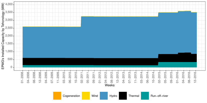
(a) EPMG’s installed capacity over time

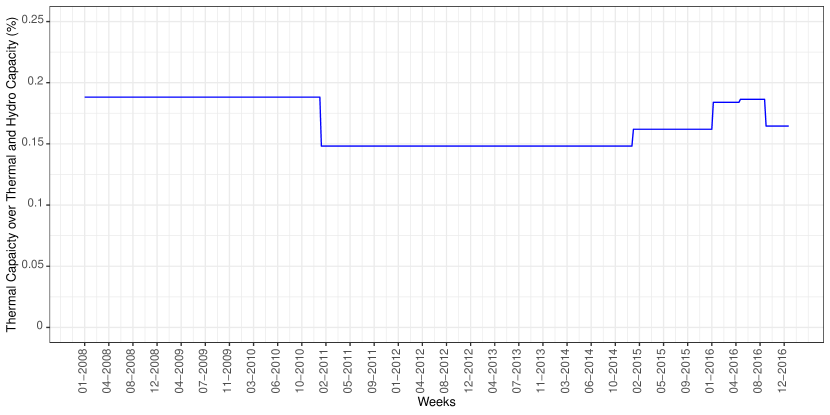
(b) Thermal capacity as a percentage of EPMG’s thermal and hydro capacity

Note: The relative contribution of different technologies to EPMG’s installed capacity over time.

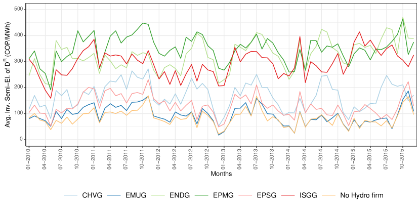
Figure F2: Monthly average inverse semi-elasticities by firm

Notes: The mean inverse elasticity for the six firms with hydro units and the average across all firms with no hydro generators (orange). The semi-elasticity is equal to the COP/MWh increase in the market-clearing price that would result from a supplier reducing the amount of energy it sells in the short-term market during hour $h$ by one percent. 2,900 COP $\simeq$ 1US$.

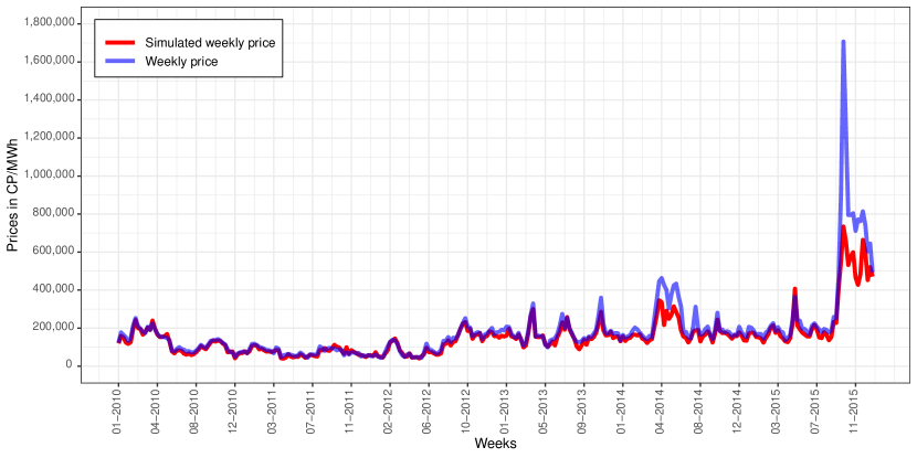
Figure F3: Model fit (30 steps for residual demand and value function

Note: The figure compares the average price over a week’s hourly markets with the market prices obtained from solving EMPG’s profit maximization problem (6.1) for each hourly market. The solver employs thirty steps to discretize the demand and the value function and 10 steps for each technology-specific supply ($M=Z=30$, $K=10$). 2,900 COP $\simeq$ 1 US$.

Appendix G Counterfactual Analyses: Tables and Figures

Figure G1: Price changes of capacity transfer to the leading firm - small transfers

Top panel: the distribution of the leader’s water inflows is on the $x$-axis

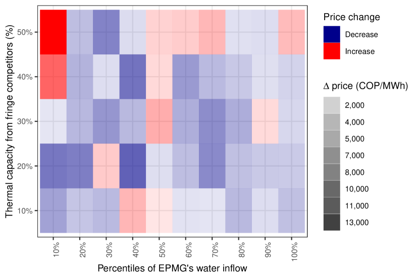
(a) Transferring $\kappa\%$ from all fringe firms

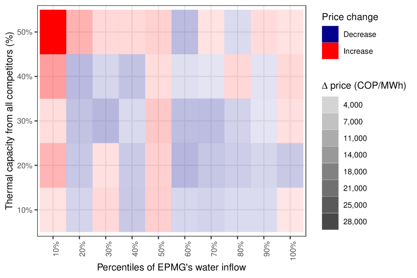
(b) Transferring $\kappa\%$ from all firms

Bottom panel: the distribution of the leader’s water stock is on the $x$-axis

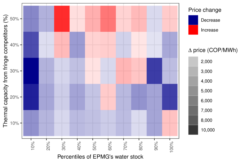
(c) Transferring $\kappa\%$ from all fringe firms

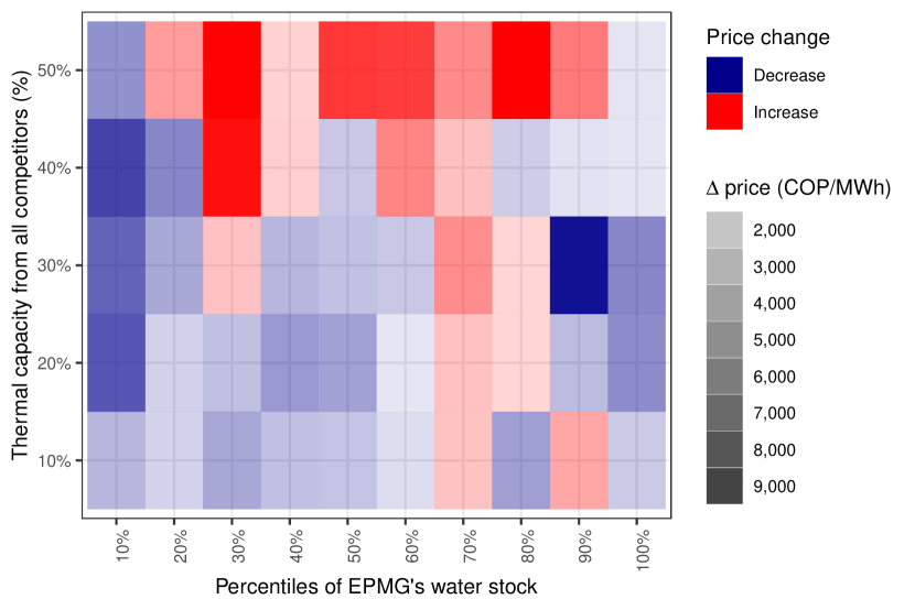
(d) Transferring $\kappa\%$ from all firms

Notes: The figure presents the results from the counterfactual exercises discussed comparing observed prices with counterfactual market prices as we endow the market leading firm with a fraction of its competitors’ thermal capacities (y-axis) for varying levels of scarcity (x-axis). Top (bottom) panels proxy scarcity by grouping markets based on the deciles of the firm’s water inflow (water stock): each cell reports the average price difference between the simulated market and the status quo with different shades of red and blue colors based on the sign and magnitude. The left (right) panels move capacity from fringe (all) firms. Unlike the plots in Figure 11, these plots cap transfer fractions to 50%. The average market price is approximately 150,000 COP/MWh. 2,900 COP $\simeq$ 1 US$.

Figure G2: Percentage price changes due to a capacity transfer to the leading firm

Top panel: the distribution of the leader’s water inflows is on the $x$-axis

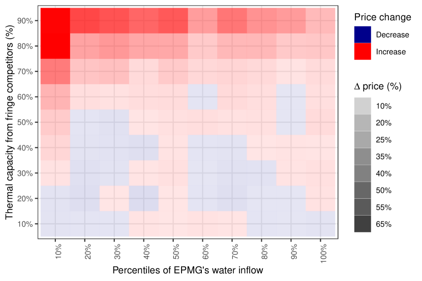
(a) Transferring $\kappa\%$ from all fringe firms

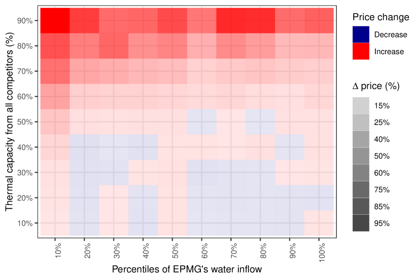
(b) Transferring $\kappa\%$ from all firms

Bottom panel: the distribution of the leader’s water stock is on the $x$-axis

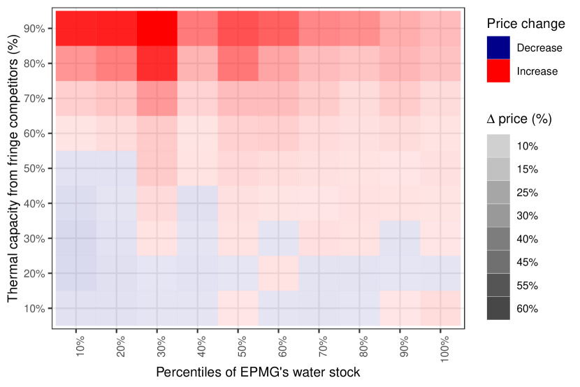
(c) Transferring $\kappa\%$ from all fringe firms

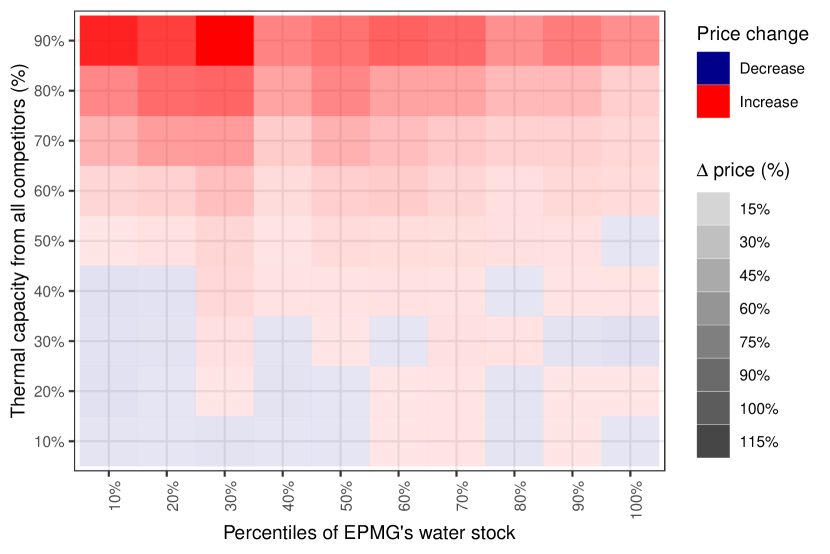
(d) Transferring $\kappa\%$ from all firms

Notes: The figure presents the results from the counterfactual exercises discussed comparing observed prices with counterfactual market prices as we endow the market leading firm with a fraction of its competitors’ thermal capacities (y-axis) for varying levels of scarcity (x-axis). Top (bottom) panels proxy scarcity by grouping markets based on the deciles of the firm’s water inflow (water stock): each cell reports the average difference between the simulated market and the status quo with different shades of red and blue colors based on the sign and magnitude. The left (right) panels move capacity from fringe (all) firms. Unlike the plots in Figure 11, which compares absolute price differences, this analysis compares percentage price differences by dividing each price difference by the baseline simulated market price ($\kappa\%=0$).

ecca sample.bib

References

- Abrell et al. (2019) Abrell, J., Rausch, S. and Streitberger, C. (2019). The economics of renewable energy support. Journal of Public Economics, 176, 94–117.
- Acemoglu et al. (2012) Acemoglu, D., Aghion, P., Bursztyn, L. and Hemous, D. (2012). The environment and directed technical change. American economic review, 102 (1), 131–166.
- Acemoglu et al. (2017) —, Kakhbod, A. and Ozdaglar, A. (2017). Competition in electricity markets with renewable energy sources. The Energy Journal, 38 (KAPSARC Special Issue).
- Acemoglu and Tahbaz-Salehi (2024) — and Tahbaz-Salehi, A. (2024). The macroeconomics of supply chain disruptions. Review of Economic Studies, p. rdae038.
- Agarwal et al. (2023) Agarwal, N., Moehring, A., Rajpurkar, P. and Salz, T. (2023). Combining human expertise with artificial intelligence: Experimental evidence from radiology. Tech. rep., National Bureau of Economic Research.
- Aghion et al. (2024) Aghion, P., Bergeaud, A., De Ridder, M. and Van Reenen, J. (2024). Lost in transition: Financial barriers to green growth.
- Alviarez et al. (2023) Alviarez, V., Fioretti, M., Kikkawa, K. and Morlacco, M. (2023). Two-sided market power in firm-to-firm trade. Tech. rep., National Bureau of Economic Research.
- Ambec and Crampes (2019) Ambec, S. and Crampes, C. (2019). Decarbonizing electricity generation with intermittent sources of energy. Journal of the Association of Environmental and Resource Economists, 6 (6), 1105–1134.
- Anderson and Hu (2008) Anderson, E. J. and Hu, X. (2008). Forward contracts and market power in an electricity market. International Journal of Industrial Organization, 26 (3), 679–694.
- Andrés-Cerezo and Fabra (2023) Andrés-Cerezo, D. and Fabra, N. (2023). Storing power: Market structure matters. The RAND Journal of Economics, 54 (1), 3–53.
- Arcidiacono and Miller (2011) Arcidiacono, P. and Miller, R. A. (2011). Conditional choice probability estimation of dynamic discrete choice models with unobserved heterogeneity. Econometrica, 79 (6), 1823–1867.
- Arcidiacono and Miller (2019) — and — (2019). Nonstationary dynamic models with finite dependence. Quantitative Economics, 10 (3), 853–890.
- Arias-Gaviria et al. (2019) Arias-Gaviria, J., Carvajal-Quintero, S. X. and Arango-Aramburo, S. (2019). Understanding dynamics and policy for renewable energy diffusion in colombia. Renewable energy, 139, 1111–1119.
- Ashenfelter et al. (2015) Ashenfelter, O. C., Hosken, D. S. and Weinberg, M. C. (2015). Efficiencies brewed: pricing and consolidation in the us beer industry. The RAND Journal of Economics, 46 (2), 328–361.
- Asker et al. (2019) Asker, J., Collard-Wexler, A. and De Loecker, J. (2019). (mis) allocation, market power, and global oil extraction. American Economic Review, 109 (4), 1568–1615.
- Atalay et al. (2019) Atalay, E., Hortaçsu, A., Li, M. J. and Syverson, C. (2019). How wide is the firm border? The Quarterly Journal of Economics, 134 (4), 1845–1882.
- Atkeson and Burstein (2008) Atkeson, A. and Burstein, A. (2008). Pricing-to-market, trade costs, and international relative prices. American Economic Review, 98 (5), 1998–2031.
- Ausubel and Cramton (2010) Ausubel, L. M. and Cramton, P. (2010). Using forward markets to improve electricity market design. Utilities Policy, 18 (4), 195–200.
- Autor et al. (2020) Autor, D., Dorn, D., Katz, L. F., Patterson, C. and Van Reenen, J. (2020). The fall of the labor share and the rise of superstar firms. The Quarterly Journal of Economics, 135 (2), 645–709.
- Balat et al. (2015) Balat, J., Carranza, J. E. and Martin, J. D. (2015). Dynamic and strategic behavior in hydropower-dominated electricity markets: Empirical evidence for colombia. Borradores de Economia, 886.
- Balat et al. (2022) —, —, —, Riascos, A. et al. (2022). The effects of changes in the regulation of the Colombian wholesale electricity market in a structural model of complex auctions. Tech. rep., Banco de la Republica de Colombia.
- Benkard et al. (2021) Benkard, C. L., Yurukoglu, A. and Zhang, A. L. (2021). Concentration in product markets. Tech. rep., National Bureau of Economic Research.
- Berger et al. (2022) Berger, D., Herkenhoff, K. and Mongey, S. (2022). Labor market power. American Economic Review, 112 (4), 1147–1193.
- Bernasconi et al. (2023) Bernasconi, M., Espinosa, M., Macchiavello, R. and Suarez, C. (2023). Relational collusion in the colombian electricity market.
- Blumsack (2023) Blumsack, S. (2023). Basic economics of power generation, transmission and distribution. The Pennsylvania State University - Energy Markets, Policy, and Regulation.
- Bodéré (2023) Bodéré, P. (2023). Dynamic spatial competition in early education: An equilibrium analysis of the preschool market in pennsylvania. Job Market Paper.
- Bonhomme et al. (2019) Bonhomme, S., Lamadon, T. and Manresa, E. (2019). A distributional framework for matched employer employee data. Econometrica, 87 (3), 699–739.
- Bornstein and Peter (2022) Bornstein, G. and Peter, A. (2022). Nonlinear pricing and misallocation.
- Braguinsky et al. (2015) Braguinsky, S., Ohyama, A., Okazaki, T. and Syverson, C. (2015). Acquisitions, productivity, and profitability: evidence from the japanese cotton spinning industry. American Economic Review, 105 (7), 2086–2119.
- Bresnahan and Suslow (1989) Bresnahan, T. F. and Suslow, V. Y. (1989). Oligopoly pricing with capacity constraints. Annales d’Économie et de Statistique, pp. 267–289.
- Bushnell (2003) Bushnell, J. (2003). A mixed complementarity model of hydrothermal electricity competition in the western united states. Operations research, 51 (1), 80–93.
- Butters et al. (2021) Butters, R. A., Dorsey, J. and Gowrisankaran, G. (2021). Soaking up the sun: Battery investment, renewable energy, and market equilibrium. Tech. rep., National Bureau of Economic Research.
- Collard-Wexler and De Loecker (2015) Collard-Wexler, A. and De Loecker, J. (2015). Reallocation and technology: Evidence from the us steel industry. American Economic Review, 105 (1), 131–171.
- Compte et al. (2002) Compte, O., Jenny, F. and Rey, P. (2002). Capacity constraints, mergers and collusion. European Economic Review, 46 (1), 1–29.
- Cramton et al. (2013) Cramton, P., Ockenfels, A. and Stoft, S. (2013). Capacity market fundamentals. economics of energy & environmental policy 2 (2): 27–46.
- Cramton and Stoft (2007) — and Stoft, S. (2007). Colombia firm energy market. In 2007 40th Annual Hawaii International Conference on System Sciences (HICSS’07), IEEE, pp. 124–124.
- Crawford et al. (2007) Crawford, G. S., Crespo, J. and Tauchen, H. (2007). Bidding asymmetries in multi-unit auctions: implications of bid function equilibria in the british spot market for electricity. International Journal of Industrial Organization, 25 (6), 1233–1268.
- de Bragança and Daglish (2016) de Bragança, G. G. F. and Daglish, T. (2016). Can market power in the electricity spot market translate into market power in the hedge market? Energy economics, 58, 11–26.
- De Frutos and Fabra (2011) De Frutos, M.-A. and Fabra, N. (2011). Endogenous capacities and price competition: The role of demand uncertainty. International Journal of Industrial Organization, 29 (4), 399–411.
- De Loecker et al. (2020) De Loecker, J., Eeckhout, J. and Unger, G. (2020). The rise of market power and the macroeconomic implications. The Quarterly Journal of Economics, 135 (2), 561–644.
- Delgado and Moreno (2004) Delgado, J. and Moreno, D. (2004). Coalition-proof supply function equilibria in oligopoly. Journal of Economic Theory, 114 (2), 231–254.
- Demirer (2022) Demirer, M. (2022). Production function estimation with factor-augmenting technology: An application to markups.
- Demirer and Karaduman (2022) — and Karaduman, O. (2022). Do mergers and acquisitions improve efficiency: Evidence from power plants. Tech. rep., Working paper.
- Durrleman and Simon (1989) Durrleman, S. and Simon, R. (1989). Flexible regression models with cubic splines. Statistics in medicine, 8 (5), 551–561.
- Elliott (2024) Elliott, J. T. (2024). Investment, emissions, and reliability in electricity markets. Tech. rep., Mimeo, John Hopkins University.
- Elliott et al. (2023) —, Houngbonon, G. V., Ivaldi, M. and Scott, P. (2023). Market structure, investment, and technical efficiencies in mobile telecommunications. Investment, and Technical Efficiencies in Mobile Telecommunications (April 25, 2023).
- Fabra and Llobet (2023) Fabra, N. and Llobet, G. (2023). Fossil fuels and renewable energy: Mix or match?
- Fioretti (2022) Fioretti, M. (2022). Caring or pretending to care? social impact, firms’ objectives, and welfare. Journal of Political Economy, 130 (11), 2898–2942.
- Fioretti et al. (2022) —, Iaria, A., Janssen, A., Mazet-Sonilhac, C. and Perrons, R. K. (2022). Innovation begets innovation and concentration: The case of upstream oil & gas in the north sea. arXiv preprint arXiv:2205.13186.
- Friberg and Romahn (2015) Friberg, R. and Romahn, A. (2015). Divestiture requirements as a tool for competition policy: A case from the swedish beer market. International journal of industrial organization, 42, 1–18.
- Froeb et al. (2003) Froeb, L., Tschantz, S. and Crooke, P. (2003). Bertrand competition with capacity constraints: mergers among parking lots. Journal of Econometrics, 113 (1), 49–67.
- Garcia et al. (2001) Garcia, A., Reitzes, J. D. and Stacchetti, E. (2001). Strategic pricing when electricity is storable. Journal of Regulatory Economics, 20 (3), 223–247.
- Gonzales et al. (2023) Gonzales, L. E., Ito, K. and Reguant, M. (2023). The investment effects of market integration: Evidence from renewable energy expansion in chile. Econometrica, 91 (5), 1659–1693.
- Gowrisankaran et al. (2022) Gowrisankaran, G., Langer, A. and Zhang, W. (2022). Policy uncertainty in the market for coal electricity: The case of air toxics standards. Tech. rep., National Bureau of Economic Research.
- Gowrisankaran et al. (2016) —, Reynolds, S. S. and Samano, M. (2016). Intermittency and the value of renewable energy. Journal of Political Economy, 124 (4), 1187–1234.
- Green and Newbery (1992) Green, R. J. and Newbery, D. M. (1992). Competition in the british electricity spot market. Journal of political economy, 100 (5), 929–953.
- Grieco et al. (2023) Grieco, P. L., Murry, C. and Yurukoglu, A. (2023). The evolution of market power in the us automobile industry. The Quarterly Journal of Economics, p. qjad047.
- Grossman (1981) Grossman, S. J. (1981). Nash equilibrium and the industrial organization of markets with large fixed costs. Econometrica: Journal of the Econometric Society, pp. 1149–1172.
- Gutiérrez and Philippon (2017) Gutiérrez, G. and Philippon, T. (2017). Declining Competition and Investment in the US. Tech. rep., National Bureau of Economic Research.
- Haar (2020) Haar, L. (2020). Inequality and renewable electricity support in the european union. In Inequality and Energy, Elsevier, pp. 189–220.
- Holmberg and Philpott (2015) Holmberg, P. and Philpott, A. (2015). Supply function equilibria in networks with transport constraints.
- Hortaçsu et al. (2018) Hortaçsu, A., Kastl, J. and Zhang, A. (2018). Bid shading and bidder surplus in the us treasury auction system. American Economic Review, 108 (1), 147–169.
- Hortaçsu et al. (2021) —, Natan, O. R., Parsley, H., Schwieg, T. and Williams, K. R. (2021). Organizational structure and pricing: Evidence from a large us airline. Tech. rep., National Bureau of Economic Research.
- Huisman et al. (2021) Huisman, R., Koolen, D. and Stet, C. (2021). Pricing forward contracts in power markets with variable renewable energy sources. Renewable Energy, 180, 1260–1265.
- IEA (2023) IEA (2023). Global co2 emissions by sector, 2019-2022.
- Jeziorski (2014) Jeziorski, P. (2014). Estimation of cost efficiencies from mergers: Application to us radio. The RAND Journal of Economics, 45 (4), 816–846.
- Jofre-Bonet and Pesendorfer (2003) Jofre-Bonet, M. and Pesendorfer, M. (2003). Estimation of a dynamic auction game. Econometrica, 71 (5), 1443–1489.
- Joskow (2011) Joskow, P. L. (2011). Comparing the costs of intermittent and dispatchable electricity generating technologies. American Economic Review, 101 (3), 238–241.
- Kalouptsidi et al. (2021) Kalouptsidi, M., Scott, P. T. and Souza-Rodrigues, E. (2021). Identification of counterfactuals in dynamic discrete choice models. Quantitative Economics, 12 (2), 351–403.
- Kastl (2011) Kastl, J. (2011). Discrete bids and empirical inference in divisible good auctions. The Review of Economic Studies, 78 (3), 974–1014.
- Klemperer and Meyer (1989) Klemperer, P. D. and Meyer, M. A. (1989). Supply function equilibria in oligopoly under uncertainty. Econometrica: Journal of the Econometric Society, pp. 1243–1277.
- Koohi-Fayegh and Rosen (2020) Koohi-Fayegh, S. and Rosen, M. A. (2020). A review of energy storage types, applications and recent developments. Journal of Energy Storage, 27, 101047.
- Kreps and Scheinkman (1983) Kreps, D. M. and Scheinkman, J. A. (1983). Quantity precommitment and bertrand competition yield cournot outcomes. The Bell Journal of Economics, pp. 326–337.
- Levenstein and Suslow (2006) Levenstein, M. C. and Suslow, V. Y. (2006). What determines cartel success? Journal of economic literature, 44 (1), 43–95.
- Lloyd (1963) Lloyd, E. (1963). A probability theory of reservoirs with serially correlated inputs. Journal of Hydrology, 1 (2), 99–128.
- McRae and Wolak (2020) McRae, S. D. and Wolak, F. A. (2020). Market power and incentive-based capacity payment mechanisms. Unpublished manuscript, Stanford University.
- Miller et al. (2021) Miller, N. H., Sheu, G. and Weinberg, M. C. (2021). Oligopolistic price leadership and mergers: The united states beer industry. American Economic Review, 111 (10), 3123–3159.
- Miller and Weinberg (2017) — and Weinberg, M. C. (2017). Understanding the price effects of the millercoors joint venture. Econometrica, 85 (6), 1763–1791.
- Morck et al. (1990) Morck, R., Shleifer, A. and Vishny, R. W. (1990). Do managerial objectives drive bad acquisitions? The journal of finance, 45 (1), 31–48.
- Moreno Rocha et al. (2022) Moreno Rocha, C. M., Milanés Batista, C., Arguello Rodríguez, W. F., Fontalvo Ballesteros, A. J. and Núñez Álvarez, J. R. (2022). Challenges and perspectives of the use of photovoltaic solar energy in colombia. International Journal of Electrical and Computer Engineering (IJECE), 12 (5), 4521–4528.
- Morlacco (2019) Morlacco, M. (2019). Market power in input markets: Theory and evidence from french manufacturing. Unpublished, March, 20, 2019.
- Murphy et al. (1992) Murphy, K. M., Shleifer, A. and Vishny, R. W. (1992). The transition to a market economy: Pitfalls of partial reform. The Quarterly Journal of Economics, 107 (3), 889–906.
- Nocke and Schutz (2018a) Nocke, V. and Schutz, N. (2018a). An aggregative games approach to merger analysis in multiproduct-firm oligopoly. Tech. rep., National Bureau of Economic Research.
- Nocke and Schutz (2018b) — and — (2018b). Multiproduct-firm oligopoly: An aggregative games approach. Econometrica, 86 (2), 523–557.
- Nocke and Whinston (2022) — and Whinston, M. D. (2022). Concentration thresholds for horizontal mergers. American Economic Review, 112 (6), 1915–1948.
- Olley and Pakes (1996) Olley, G. S. and Pakes, A. (1996). The dynamics of productivity in the telecommunications equipment industry. Econometrica, 64 (6), 1263–1297.
- Paul (2001) Paul, C. J. M. (2001). Cost economies and market power: the case of the us meat packing industry. Review of Economics and Statistics, 83 (3), 531–540.
- Pesaran and Shin (1995) Pesaran, M. H. and Shin, Y. (1995). An autoregressive distributed-lag modelling approach to cointegration analysis. Econometrics and Economic Theory in the 20th Century, pp. 371–413.
- Reguant (2014) Reguant, M. (2014). Complementary bidding mechanisms and startup costs in electricity markets. The Review of Economic Studies, 81 (4), 1708–1742.
- Reguant (2019) — (2019). The efficiency and sectoral distributional impacts of large-scale renewable energy policies. Journal of the Association of Environmental and Resource Economists, 6 (S1), S129–S168.
- Robinson (1953) Robinson, J. (1953). The production function and the theory of capital. The Review of Economic Studies, 21 (2), 81–106.
- Ruddell et al. (2017) Ruddell, K., Philpott, A. B. and Downward, A. (2017). Supply function equilibrium with taxed benefits. Operations Research, 65 (1), 1–18.
- Rueda-Bayona et al. (2019) Rueda-Bayona, J. G., Guzmán, A., Eras, J. J. C., Silva-Casarín, R., Bastidas-Arteaga, E. and Horrillo-Caraballo, J. (2019). Renewables energies in colombia and the opportunity for the offshore wind technology. Journal of Cleaner Production, 220, 529–543.
- Ryan (2021) Ryan, N. (2021). The competitive effects of transmission infrastructure in the indian electricity market. American Economic Journal: Microeconomics, 13 (2), 202–242.
- Schmalensee (2019) Schmalensee, R. (2019). On the efficiency of competitive energy storage. Available at SSRN 3405058.
- SEI (2023) SEI (2023). Solar and wind power in Colombia: 2022 policy overview.
- Solow (1955) Solow, R. M. (1955). The production function and the theory of capital. The Review of Economic Studies, 23 (2), 101–108.
- Sraffa (1960) Sraffa, P. (1960). Production of Commodities by Means of Commodities: Prelude to a Critique of Economic Theory. Cambridge University Press.
- Staiger and Wolak (1992) Staiger, R. W. and Wolak, F. A. (1992). Collusive pricing with capacity constraints in the presence of demand uncertainty. The RAND Journal of Economics, pp. 203–220.
- Stone and Koo (1985) Stone, C. J. and Koo, C.-Y. (1985). Additive splines in statistics. Proceedings of the American Statistical Association Original pagination is p, 45, 48.
- Sweeting (2013) Sweeting, A. (2013). Dynamic product positioning in differentiated product markets: The effect of fees for musical performance rights on the commercial radio industry. Econometrica, 81 (5), 1763–1803.
- Vehviläinen (2021) Vehviläinen, I. (2021). Joint assessment of generation adequacy with intermittent renewables and hydro storage: A case study in finland. Electric Power Systems Research, 199, 107385.
- Verde (2008) Verde, S. (2008). Everybody merges with somebody—the wave of m&as in the energy industry and the eu merger policy. Energy policy, 36 (3), 1125–1133.
- Vives (2011) Vives, X. (2011). Strategic supply function competition with private information. Econometrica, 79 (6), 1919–1966.
- Wilson (1979) Wilson, R. (1979). Auctions of shares. The Quarterly Journal of Economics, 93 (4), 675–689.
- Wolak (2007) Wolak, F. A. (2007). Quantifying the supply-side benefits from forward contracting in wholesale electricity markets. Journal of Applied Econometrics, 22 (7), 1179–1209.