Enhancement of Over-the-Air Federated Learning by Using AI-based Fluid Antenna System
Abstract
This letter investigates an over-the-air federated learning (OTA-FL) system that employs fluid antennas (FAs) at the access point (AP) to enhance learning performance by leveraging the additional degrees of freedom provided by antenna mobility. First, we analyze the convergence of the OTA-FL system and derive the optimality gap to illustrate the influence of FAs on learning performance. Then, we formulate a nonconvex optimization problem to minimize the optimality gap by jointly optimizing the positions of the FAs and the beamforming vector. To address the dynamic environment, we cast this optimization problem as a Markov decision process (MDP) and propose the recurrent deep deterministic policy gradient (RDPG) algorithm. Finally, extensive simulations show that the FA-assisted OTA-FL system outperforms systems with fixed-position antennas and that the RDPG algorithm surpasses the existing methods.
Index Terms:
Optimality gap, Over-the-air federated learning, Fluid antenna, Deep reinforcement learning.I Introduction
Federated learning (FL) has gained significant prominence in the field of machine learning in recent years due to its decentralized framework and robust privacy protection measures. FL leverages the computational capabilities of edge devices to collectively train a unified global model, all while ensuring that sensitive locally stored data remains confidential. This approach is particularly suitable for applications in various Internet of Mobile Things (IoMT) scenarios, including the Internet of Drones (IoD)[1] and mobile crowd sensing[2], among others. To mitigate communication latency and costs associated with FL implementation, over-the-air computation (AirComp) for model aggregation has emerged as a promising approach. It leverages the superposition property of wireless multiple access channels (MAC) [3]. However, the performance of model aggregation in over-the-air FL (OTA-FL) is severely affected by adverse wireless propagation channel conditions, especially in massive mobile IoT scenarios.
To address this challenge, previous research has extensively explored the integration of intelligent reflecting surfaces (IRSs) into OTA-FL to achieve reliable model aggregation. This is accomplished by reconfiguring wireless channels through adjusting the passive reflecting coefficients of the IRS [3]. Additionally, other studies have investigated beamforming techniques at the receiver server to enhance OTA-FL performance by leveraging the degrees of freedom (DoF) in the spatial domain [4]. However, the fixed positions of receiver antennas can impose limitations on the potential gains from beamforming. To overcome these limitations, we propose the use of fluid antennas (FAs) in OTA-FL to dynamically manipulate wireless channel conditions through adaptive movement of antennas. Unlike fixed-position antennas (FPA), FAs offer the capability to reshape channel environments, thereby introducing new DoFs to enhance OTA-FL performance [5]. Previous studies have demonstrated the superior performance of FAs over traditional FPAs in various communication systems, including AirComp systems [6], multi-user uplink communications [7, 5, 8], and mobile edge computing [9]. Moreover, FAs have been investigated to maximize network sum-rate in multiple access communication systems through deep reinforcement learning (DRL) [10]. However, the integration of FAs into OTA-FL systems has not yet been addressed in current academic literature to the best of our knowledge.
In this paper, we propose the integration of FA systems with OTA-FL to enhance convergence performance. Our objective is to minimize the optimality gap through joint optimization of the beamforming vector and the antenna position vector at the access point (AP) under practical dynamic conditions [11]. First, we derive the optimality gap between the actual loss and the optimal loss for OTA-FL to quantify the impact of the beamforming vector and antenna positioning. Subsequently, based on the convergence analysis, we formulate a non-convex optimization problem to enhance learning performance. We then reformulate it as a Markov decision process (MDP) and leverage deep reinforcement learning (DRL) techniques suitable for dynamic environments. We introduce the recurrent deep deterministic policy gradient (RDPG) algorithm, with actor and critic networks specifically designed to capture the temporal correlation of state features, enabling real-time decisions under dynamic conditions. Extensive simulations are undertaken to evaluate the performance of the integrated FAs in OTA-FL systems compared to FPA, and the performance of the proposed RDPG algorithm in comparison to standard DRL algorithms such as soft actor-critic (SAC) and deep deterministic policy gradient (DDPG). Simulation results indicate that the proposed RDPG algorithm outperforms both SAC and DDPG methods in terms of performance and stability in both scenarios. Furthermore, the FA-assisted OTA-FL system consistently outperforms the FPA scenarios.
Notations: Italicized letters represent scalars, while boldface letters denote vectors. is the transpose, the conjugate transpose, and the expectation operation. signifies the magnitude of a scalar or the cardinality of a set. The Euclidean norm of a vector is represented by .
II System Model
We consider an OTA-FL system comprising single-antenna user equipment (UE) devices, denoted as , . These devices could be include mobile IoT devices, UAVs, drones, or similar entities. The UEs are randomly distributed and move dynamically within a designated area of interest, where they collect local data samples. These samples are collaboratively utilized to train a global model at an AP equipped with FAs.
II-A OTA-FL Model
We consider an OTA-FL framework with full participation that executes sequential actions at each iteration over training rounds as follows:
-
•
Global model broadcast: The AP broadcasts the current global model to all UEs, where represents the dimensionality of the model parameter space.
-
•
Local model update: Each UE updates its local model using the gradient descent algorithm as , where is the learning rate, represents the gradient of the local loss function, and is the local dataset for with a local dataset size denoted by .
-
•
Model aggregation: Each UE transmits its local model to the AP, which then performs aggregation by averaging to update the global model as:
(1)
The procedure continues iteratively until reaching the maximum specified number of outer iterations.
II-B Communication Model
We consider the uploading phase within the OTA-FL system, where each UE synchronously transmits its updated model parameters to the AP. The AP is equipped with an array of FAs, facilitating the adjustment of each FA along a one-dimensional line segment that spans a length of . Each FA’s position is constrained within the interval with a minimum distance between adjacent FAs to prevent antenna coupling. The collective locations of all FAs are represented as the vector , with their movement along one dimension restricted by . For the purposes of brevity and clarity, time indices are omitted in this subsection. Assuming line-of-sight (LoS) propagation conditions, the channel between the and the AP, represented by , is given by
| (2) |
where , , and denote the path loss at the reference distance, the wavelength, and the path loss exponent, respectively. and represent the distance between the FAs and and the angle of arrival (AoA) of the LoS path, respectively, which are determined by the location of the UEs in each training round. In this system, we assume each UE moves within an designated area and then transmits model parameters from a stationary position [2]. Moreover, given that the signal path length significantly exceeds the FA movement area, the far field condition between the AP and UEs is assumed. Consequently, and are treated as constants during transmission, regardless of FA positional changes [9, 7].
The AP receives the local model parameters from all UEs in the -th training round as:
| (3) |
where, denotes the transmission power factor for the -th UE, and represents an additive white Gaussian noise (AWGN) matrix with elements following a complex normal distribution .
The aggregated model parameter vector, , in the -th training round is estimated by conducting post-processing on the received signal at the AP as follows:
| (4) | ||||
where, denotes the beamforming vector at the AP, and represents the scaling factor for signal amplitude alignment.
According to [4, 3], in order to minimize the mean square error (MSE) in the OTA-FL system, the transmit power factor in each client is designed as follows:
| (5) |
We consider that the transmission power allocated to each does not exceed the maximum transmission power limit , expressed as:
| (6) |
Moreover, under the assumption of full participation in FL to adhere to the maximum power budget for each client, the upper bound of must satisfy the following condition:
| (7) |
III Convergence Analysis
In order to facilitate our analysis of convergence, we incorporate the following commonly accepted assumptions as discussed in [3, 1, 12]:
Assumption 1: The global loss function is -smooth. Namely, for any given model parameters , there exists a nonnegative constant , such that
| (8) |
Assumption 2: The loss function satisfies the Polyak-Lojasiewicz inequality, where denotes the optimal global loss value and , as follows:
| (9) |
Assumption 3: The upper limit of the model parameter for is denoted as . This ensures:
| (10) |
Theorm 1: Under the conditions outlined in Assumptions III, III, and III, and setting the learning rate to , the optimality gap after rounds of training is bounded as follows:
| (11) | ||||
where, and can be represented as follows:
| (12) |
| (13) |
Proof:
See Appendix. ∎
IV Problem Formulation
In this paper, our objective is to enhance learning performance in OTA-FL through the design of FA systems within dynamic environments. According to Theorem III, the optimality gap is influenced by the configuration of the beamforming vector and the FA locations in the training iterations. Thus, we formulate an optimization problem to jointly optimize and for all , aiming to minimize the total optimality gap as follows:
| (14) | ||||
where, constrains the permissible range for FA locations, determines the order of FA placements, and enforces a minimum separation distance between adjacent FAs.
Due to the non-convex nature of the objective function and the stochasticity inherent in the dynamic environment, particularly in massive mobile IoT scenarios, traditional optimization methods face challenges in solving the original intractable problem . In order to tackle this issue, we propose transforming problem into an online optimization problem, subsequently reformulating it as an MDP. Based on Theorem III, the optimality gap at the -th training round, denoted as , is bounded as follows:
| (15) | ||||
where (15) indicates that when and the initial optimality gap are known, the optimality gap is determined by and the previous optimality gap . Thus, the problem of minimizing the optimality gap after communication rounds can be transformed into minimizing in each round. This reformulation is expressed as follows:
| (16) | |||
V Proposed DRL Algorithm
To address Problem , we deploy a DRL agent on the AP to learn an optimal decision policy that simultaneously optimizes the beamforming vector and the FA locations in each training round in order to minimize . Details of the MDP are provided below:
-
•
State Space: The state space at time slot consists of the distances between the FAs and the , and the AoA of the LoS paths , . The state space can be expressed as: .
-
•
Action space: The action space at each time slot comprises the beamforming vector and the locations of the FAs. Consequently, the action space at time slot can be expressed as:
(17) -
•
Reward function: Based on (12), in order to minimize , the reward function can be formulated as:
(18) where, the constants and are negative values that require tuning during the simulation process to achieve better convergence. Notably, the reward function is formulated as a negative value. Therefore, by maximizing this (negative) reward, the agent effectively minimizes .
Since the action space is continuous, we cannot use model-free value-based DRL algorithms such as deep Q-network (DQN), as they can only handle discrete action spaces. Instead, we utilize policy gradient-based reinforcement learning methods. The DDPG algorithm is a suitable off-policy actor-critic approach capable of managing continuous action spaces. However, the fully-connected deep neural networks (DNNs) employed in conventional DDPG are inadequate for capturing the temporal patterns of environmental dynamics, such as user mobility [13, 11]. Therefore, we adjust the RDPG approach by incorporating long short-term memory (LSTM) into the DDPG architecture to exploit temporal state patterns and adapt continuously to environmental dynamics.
The proposed RDPG algorithm utilizes four neural networks: an Actor Network (policy network) denoted by with parameter , which determines actions based on states , where is a random process added to actions for exploration; a Critic Network (Q-network) with parameters that computes Q-values for state-action pairs; a Target Actor Network, which is an older version of the actor network; and a Target Critic Network, which is an older version of the critic network.
In our optimization problem, the objective is to minimize the optimality gap by maximizing the expected reward in each training round. The goal of the RDPG, given the state and action , is to identify a policy that maximizes the expected cumulative reward, defined as:
| (19) |
to achieve this, the Actor Network is optimized based on the gradient of the objective function as follows:
| (20) |
while the critic network is trained to minimize the loss function relative to the target value , defined as:
| (21) |
The proposed RDPG method is described in Algorithm 1.
VI Simulation Results
In this section, we provide numerical results illustrating how combining FA arrays with the proposed RDPG algorithm can improve OTA-FL learning performance. We consider the distance between users and the AP to be uniformly distributed in the range m, and the AoAs to be uniformly distributed over rad. The parameters for the FA arrays are set with and . The RDPG algorithm is configured with a learning rate of 0.0005, a replay buffer size of , a batch size of 64, a soft update parameter of 0.001, and a discount factor of 0.9. For performance evaluation, we consider two comparisons. Initially, we evaluate the performance of FA relative to FPA with a predetermined location vector . Subsequently, we compare the proposed RDPG algorithm with SAC [14] and DDPG [13], which are conventional DRL algorithms. Learning performance is evaluated by computing the average rewards over 100 episodes, which is determined at episode by employing the formula , where signifies the mean reward of episode .
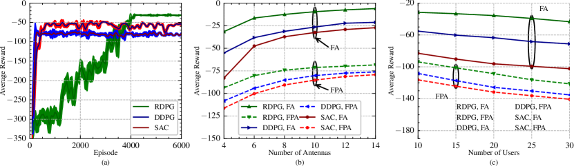
Fig. 1 (a) demonstrates the convergence characteristics of different DRL algorithms, depicting the average rewards with solid curves and showing the standard deviations as shaded regions. The RDPG algorithm exhibits higher average rewards and lower variance compared to standard DRLs, demonstrating superior performance and improved stability in dynamic environments.
To assess the performance of the proposed algorithms across varying numbers of antennas, we kept the number of clients fixed and varied the antenna count in both the FA and FPA scenarios. As depicted in Fig. 1 (b), the average reward performance of all DRL methods improves with increasing , although this improvement diminishes as continues to increase. Furthermore, due to the increased DoF provided by antenna adjustments in FA systems, FAs consistently outperform FPAs at all values . Moreover, RDPG demonstrating superior performance over other DRL algorithms.
Fig. 1(c) provides a detailed comparison of the performance of FAs and the RDPG algorithm across varying numbers of users. It is evident from the results that as the number of users increases, there is a noticeable decrease in performance for both FA and FPA scenarios. This decline is attributed to the increased challenge of optimizing the beamforming vector and the antenna position vector of the AP in the presence of more dynamic users. Despite these challenges, FAs consistently outperform FPAs in all tested scenarios, highlighting the efficacy of FAs in enhancing OTA-FL system performance. Moreover, the RDPG algorithm consistently exhibits superior performance compared to other optimization methods in mitigating the adverse effects of dynamic user dynamics on system performance.
VII Conclusion
In this study, we investigated the integration of FAs into AP to improve the performance of OTA-FL systems. Our convergence analysis highlighted the significant impact of FA positions and the beamforming vector on the optimality gap. We addressed this issue with a non-convex optimization problem and proposed the RDPG algorithm for real-time optimization. Through simulations, we demonstrated that the OTA-FL system enhanced by FAs outperformed conventional FPA systems. Moreover, RDPG demonstrates superior performance and stability compared to existing methods, validating its effectiveness in dynamic environments.
Proof of Theorem III
In the -th communication round, the global model update is formulated by integrating (5) into (4), as follows:
| (22) | ||||
where, is the global gradient and is the model aggregation error caused by wireless communication in the -th communication round. By applying (22) in Assumption III, and setting , after taking expectation, we have:
| (23) | ||||
By applying the upper bound of based on (LABEL:eta) and employing Assumption III and III, then subtracting from both sides of (23), we have:
| (24) |
By recursively operating on (24) and using the definitions of and in (12) and (13), the cumulative optimality gap is calculated as follows:
| (25) | ||||
Proof of Theorem III is complete.
Appendix A References Section
References
- [1] J. Yao and et al., “Secure federated learning by power control for internet of drones,” IEEE Transactions on Cognitive Communications and Networking, vol. 7, no. 4, pp. 1021–1031, Apr. 2021.
- [2] Y. Wang and et al., “Learning in the air: Secure federated learning for UAV-assisted crowdsensing,” IEEE Transactions on Network Science and Engineering, vol. 8, no. 2, pp. 1055–1069, Aug. 2020.
- [3] Z. Wang and et al., “Federated learning via intelligent reflecting surface,” IEEE Transactions on Wireless Communications, vol. 21, no. 2, pp. 808–822, Jul. 2021.
- [4] C. Chen and et al., “Joint client selection and receive beamforming for over-the-air federated learning with energy harvesting,” IEEE Open Journal of the Communications Society, vol. 4, pp. 1127–1140, May. 2023.
- [5] G. Hu and et al., “Fluid Antennas-Enabled Multiuser Uplink: A Low-Complexity Gradient Descent for Total Transmit Power Minimization,” IEEE Communications Letters, vol. 28, no. 3, pp. 602–606, Jan. 2024.
- [6] D. Zhang and et al., “Fluid antenna array enhanced over-the-air computation,” IEEE Wireless Communications Letters, vol. 13, no. 6, pp. 1541–1545, Mar. 2024.
- [7] H. Qin and et al., “Antenna positioning and beamforming design for fluid antenna-assisted multi-user downlink communications,” IEEE Wireless Communications Letters, vol. 13, pp. 1073–1077, Jan. 2024.
- [8] Z. Cheng and et al., “Sum-rate maximization for fluid antenna enabled multiuser communications,” IEEE Communications Letters, vol. 28, no. 5, pp. 1206–1210, Mar. 2024.
- [9] Y. Zuo and et al., “Fluid Antenna for Mobile Edge Computing,” IEEE Communications Letters, May. 2024.
- [10] N. Waqar and et al., “Opportunistic fluid antenna multiple access via team-inspired reinforcement learning,” IEEE Transactions on Wireless Communications, Apr. 2024.
- [11] X. Fan and et al., “UAV-Enabled Federated Learning in Dynamic Environments: Efficiency and Security Trade-off,” IEEE Transactions on Vehicular Technology, vol. 73, no. 5, pp. 6993–7006, Dec. 2023.
- [12] X. Cao and et al., “Transmission power control for over-the-air federated averaging at network edge,” IEEE Journal on Selected Areas in Communications, vol. 40, no. 5, pp. 1571–1586, Jan. 2022.
- [13] S. Sheikhzadeh and et al., “AI-based secure NOMA and cognitive radio-enabled green communications: Channel state information and battery value uncertainties,” IEEE Transactions on Green Communications and Networking, vol. 6, no. 2, pp. 1037–1054, Dec. 2021.
- [14] V. Konda and et al., “Actor-critic algorithms,” Advances in neural information processing systems, vol. 12, pp. 1008–1014, Dec. 1999.