Testing the equivalence between the planar Gross-Neveu and Thirring models at $N=1$

Abstract

It is known that the Fierz identities predict that the Gross-Neveu and Thirring models should be equivalent when describing systems composed of a single fermionic flavor, $N=1$. Here, we consider the planar version of both models within the framework of the optimized perturbation theory at the two loop level, in order to verify if the predicted equivalence emerges explicitly when different temperature and density regimes are considered. At vanishing densities, our results indicate that both models indeed describe exactly the same thermodynamics, provided that $N=1$. However, at finite chemical potentials we find that the $N=1$ Fierz equivalence no longer holds. After examining the relevant free energies, we have identified the contributions which lead to this puzzling discrepancy. Finally, we discuss different frameworks in which this (so far open) problem could be further understood and eventually circumvented.

I Introduction

Relativistic four-fermion theories are widely used to describe different physical scenarios in condensed matter and particle physics. In the latter case, the Nambu–Jona-Lasinio (NJL) Nambu:1961tp ; Nambu:1961fr model has been successfully used as an effective model to describe the QCD chiral phase transition. As far as condensed matter is concerned, the planar Gross-Neveu (GN) Gross:1974jv and Thirring Thirring:1958in models have been employed to describe low-energy electronic properties of materials like graphene Hands:2008id ; Ebert:2015hva ; Ebert:2018dzs , high-temperature superconductors Zhukovsky:2017hzo ; Klimenko:2012qi , Weyl semimetals Gomes:2021nem ; Gomes:2022dmf ; Gomes:2023vvu , among many other systems Caldas:2008zz ; Caldas:2009zz ; Ramos:2013aia ; Klimenko:2013gua ; Khunjua:2021fus ; Gubaeva:2022feb ; Khunjua:2022kxf .

The basic difference between the GN and Thirring models arises from the matrix structure of the four-fermion channel, $(\bar{\psi}_{k}\Gamma\psi_{k})^{2}$ ($k=1,...,N$), considered in each case. This channel has a scalar structure ($\Gamma\equiv\mathbbm{1}$) in the GN case, while a vector structure ($\Gamma\equiv\gamma^{\mu}$) is adopted within the Thirring Lagrangian density. Despite this important physical difference, the use of Fierz identities Fierz:1937wjm ; Nieves:2003in allows us to conclude that both models turn out to be equivalent when describing systems composed by a single fermionic flavor, $N=1$ (see, e.g. Ref. Rosenstein:1988zf and, for a recent discussion, Ref. Wipf:2022hqd ). This result offers an additional opportunity to explicitly test non-perturbative methods which are able to incorporate finite $N$ corrections. In this context, it is worth to mention that some of the traditional analytical methods used to study these models, such as the large-$N$ (or mean-field) approximation, cannot reliably accommodate for small values of $N$, which precludes in explicitly verifying the equivalence between the models. This represents a special issue when trying to compare the thermodynamical properties of both models. In addition, one could recur to lattice simulations in order to explicitly verify the equivalence predicted by means of the Fierz identities. However, within the domain of finite fermionic densities, these numerical simulations are plagued by the well documented sign problem Karsch:2001cy ; Muroya:2003qs . This fact produces an unfortunate situation, since the density is usually crucial for the description of many condensed matter systems. To circumvent these difficulties, one must resort to alternative analytical non-perturbative approximations that are capable of going beyond the large-$N$ limit. In this context, the optimized perturbation theory (OPT) Okopinska:1987hp ; Duncan:1988hw (see also, e.g., Ref. Yukalov:2019nhu for a recent review), offers a convenient and simple enough framework to study such a problem since, within this method, contributions of order $1/N$ typically already appear at its first non-trivial order.

The OPT has been very successful in the description of phase transitions within four-fermion theories such as the ones described by the NJL and GN models Kneur:2007vj ; Kneur:2007vm ; Kneur:2010yv ; Kneur:2013cva . Here, this approximation will be employed to describe the thermodynamic potential of the 2+1 $d$ GN and Thirring models including the crucial first $1/N$ contributions. Although the OPT results for the GN case to be considered here were originally obtained in Refs. Kneur:2007vj ; Kneur:2007vm , the present work represents the first OPT application to the Thirring model as far as we are aware of. As we shall demonstrate, the expected equivalence between the models can be explicitly confirmed at all temperatures and vanishing densities. On the other hand, at least at the first order in the OPT method considered here, the equivalence does not seem to hold exactly when finite chemical potential values are considered. We offer a discussion about the possible reasons for this unexpected result.

The manuscript is organized as follows. In Sec. II, we present both models considered in this paper, namely, the GN and Thirring models. In Sec. III, we obtain the OPT Lagrangian densities for the two models. The corresponding effective potentials for each model are presented in Sec. IV. The optimization procedure is implemented in Sec. V. The thermodynamical results are presented and discussed in Sec. VI. Finally, in Sec. VII we present our concluding remarks. Two appendices are also included to show some of the more technical details.

II The Models

The GN Gross:1974jv and Thirring Thirring:1958in models can be described using a unified notation, $\Gamma$, which represents the identity for the GN model and $\gamma^{\mu}$ for the Thirring model. The Lagrangian density for a fermion field $\psi_{k}\ (k=1,\ldots,N)$ describing both models can then be written as

$$\mathcal{L}=\bar{\psi}_{k}(i\not{\partial})\psi_{k}+m_{f}\bar{\psi}_{k}\psi_{k}+\frac{\lambda}{2N}(\bar{\psi}_{k}\Gamma\psi_{k})^{2},$$ (1)

where the summation over fermionic species, $\bar{\psi}_{k}\Gamma\psi_{k}=\sum_{k=1}^{N}\bar{\psi}_{k}\Gamma\psi_{k}$, is implied. When $m_{f}=0$, the Lagrangian density given by Eq. (1) is invariant under the discrete chiral symmetry transformation $\psi\rightarrow\gamma_{5}\psi$. At finite temperatures and densities, the grand partition function is

$$Z(\beta,\mu)=\operatorname{Tr}\exp[-\beta(H-\mu Q)],$$ (2)

where $\beta$ is the inverse temperature, $\mu$ the chemical potential, $H$ the Hamiltonian, and $Q=\int dx\;\bar{\psi}_{k}\gamma_{0}\psi_{k}$ is the conserved charge. In the Euclidean formalism and in terms of functional integration over the fermion fields, we have that

$$Z(\beta,\mu)=\int\prod_{k=1}^{N}D\bar{\psi}_{k}D\psi_{k}\exp\left\{-S_{E}\left[\bar{\psi}_{k},\psi_{k}\right]\right\},$$ (3)

with the Euclidean action given by

$$S_{E}\left[\bar{\psi}_{k},\psi_{k}\right] = \int_{0}^{\beta}d\tau\int dx\left[\bar{\psi}_{k}\left(\not{\partial}+\mu\gamma_{0}-m_{f}\right)\psi_{k}\right.$$ (4)

$$- \left.\frac{\lambda}{2N}(\bar{\psi}_{k}\Gamma\psi_{k})^{2}\right],$$

and fermion fields satisfying anti-periodic boundary conditions: $\psi_{k}(x,\tau)=-\psi_{k}(x,\tau+\beta)$.

The work in Ref. Wipf:2022hqd has employed the Fierz identities to show the equivalence between the $N=1$ Thirring and GN models in both $2d$ and $3d$. The Fierz identities are mathematical transformations that rearrange products of spinor bilinears into different combinations, revealing underlying symmetries and equivalences between seemingly distinct interaction terms Fierz:1937wjm ; Nieves:2003in . This equivalence is expressed here as

$$\frac{\lambda}{2N}\left(\bar{\psi}\gamma^{\mu}\psi\right)^{2}=-\frac{d\lambda}{2N}(\bar{\psi}\psi)^{2},\quad N=1,$$ (5)

where $d$ represents the spacetime dimension, which can be either $d=2$ or $d=3$. This result highlights that, for a single fermion flavor, the interaction term in the Thirring model, which involves a vector current-current interaction, is mathematically equivalent to the scalar-scalar interaction term in the GN model. Such duality arises due to the specific properties of the spinor components in both two and three dimensions. Since our work focuses on the three-dimensional case with $N=1$, this equivalence is directly relevant to our study.

III Interpolated Theories

The implementation of the OPT technique follows a deformation of the original Lagrangian density by adding and subtracting a Gaussian term $(1-\delta)\eta\overline{\psi}_{k}\psi_{k}$, while the coupling constant, $\lambda$, which parametrizes the four-fermion vertex becomes $\delta\lambda$. A given physical quantity can then be evaluated as a perturbative series in powers of $\delta$. Once the series is truncated at a given order-$\delta^{k}$ the bookkeeping parameter is set to its original value, $\delta=1$, while the mass parameter ($\eta$) is usually optimized in a variational fashion. In general, this procedure allows for a resummation of the original perturbative series, generating non-perturbative results Pinto:1999py ; Pinto:1999pg ; Farias:2008fs ; Rosa:2016czs ; Farias:2021ult . One of the advantages of such a method is that originally massless theories, such as the ones to be considered here, are well-behaved in the infrared limit since the variational mass parameter ($\eta$) naturally regularizes all integrals at vanishing momenta. Another welcome feature is that the actual evaluations are carried out using the usual perturbation theory framework (including the renormalization procedure).

The application of the OPT method to the Thirring model follows a similar procedure to the one used for the GN model considered in many previous works Kneur:2007vj ; Kneur:2007vm ; Kneur:2013cva . The modified Lagrangian density for this model, including a linear interpolation with the fictitious parameter $\delta$ of the OPT prescription, is given by

$$\mathcal{L}_{\text{Th}}=\bar{\psi}_{k}(i\not{\partial})\psi_{k}+(1-\delta)\eta\bar{\psi}_{k}\psi_{k}+\frac{\delta\lambda}{2N}\left(\bar{\psi}_{k}\gamma^{\mu}\psi_{k}\right)^{2}.$$ (6)

As $\delta$ varies from 0 to 1, the theory interpolates from free fermions to the original interacting theory. This formulation allows the application of the OPT method to derive non-perturbative results for the Thirring model, similar to the approach taken for the GN model Kneur:2007vj ; Kneur:2007vm ; Kneur:2013cva . The Lagrangian density (6) can also more conveniently be expressed in terms of an auxiliary vector field $v^{\mu}$ by adding the term

$$-\frac{\delta N}{2\lambda}\left(v^{\mu}+\frac{\lambda}{N}\bar{\psi}_{k}\gamma^{\mu}\psi_{k}\right)^{2}\,,$$ (7)

to it. This leads us to the interpolated model,

$$\mathcal{L}_{\text{Th}}=\bar{\psi}_{k}(i\not{\partial})\psi_{k}-\bar{\psi}_{k}\left[\eta-\delta\left(\eta-\not{v}\right)\right]\psi_{k}-\frac{\delta N}{2\lambda}v^{\mu}v_{\mu},$$ (8)

where $\not{v}=\gamma^{\mu}v_{\mu}$. The original GN Lagrangian density, when deformed in the same way, leads to Kneur:2007vm

$$\mathcal{L}_{\text{GN}}=\bar{\psi}_{k}(i\not{\partial})\psi_{k}-\bar{\psi}_{k}[\eta-\delta(\eta-\sigma)]\psi_{k}-\frac{\delta N}{2\lambda}\sigma^{2},$$ (9)

where $\sigma$ is an (auxiliary) scalar field. Note that the Euler-Lagrange equations for Eqs. (8) and (9) set the auxiliary fields to $v^{\mu}=-({\lambda}/{N})\bar{\psi}_{k}\gamma^{\mu}\psi_{k}$ and $\sigma=-({\lambda}/{N})\bar{\psi}_{k}\psi_{k}$, respectively.

From the interpolated Lagrangian densities, Eqs. (8) and (9), we can derive the new Feynman rules in Minkowski space: each Yukawa vertex carries a factor $-i\delta\Gamma$, while both auxiliary field propagators read $-i\lambda/(N\delta)$. At the same time, the fermion propagator now reads $i(\not{p}-\eta+i\epsilon)^{-1}$ and a novel (quadratic) vertex contributes with $-i\delta\eta$.

The optimization process starts by using some variational principle, such as the widely used principle of minimal sensitivity (PMS) Stevenson:1981vj . The PMS criterion consists of applying the following variational condition to the physical quantity under consideration, which in the present case is taken to be the effective potential. This means that the optimal variational mass must satisfy the relation

$$\left.\frac{dV_{\rm eff}}{d\eta}\right|_{\overline{\eta}}=0\,,$$ (10)

as we shall demonstrate in the next section.

IV The effective potentials in the OPT scheme

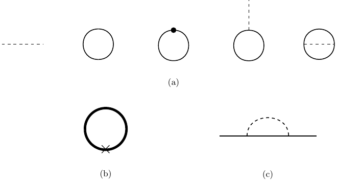
Figure 1: (a) Diagrams contributing to the effective potential at order-$\delta$. The external dashed line represents the auxiliary fields $\sigma$ (GN), or $v^{\mu}$ (Thirring). The internal dashed line represents the respective propagators associated with each auxiliary field. The thin solid lines represent the (bare) fermion propagator in terms of $\eta$. The Yukawa vertex is proportional to $\gamma_{\mu}$ (Thirring) or to the identity matrix $\mathbbm{1}$ (GN). (b) Diagram representing the quark condensate and the fermion number density when x” respectively represents the identity or $\gamma_{0}$. The thick continuous line represents the dressed (optimized) fermion propagator, in terms of $\overline{\eta}$ (c) The exchange (self-energy) fermionic one-loop contribution of order $\delta/N$.

Let us start by recalling that the Fierz equivalence relation, Eq. (5), requires that the four-fermion vertices describing the Thirring and GN models have opposite signs. Since we are interested in studying the breaking/restoration of chiral symmetry, it is convenient to perform the replacement $\lambda\to|\lambda|$ in Eq. (8) and $\lambda\to-|\lambda|$ in Eq. (9). These particular choices can be justified by recalling that, within the planar GN model, chiral symmetry breaking only occurs when the coupling is negative. Furthermore, since the coupling $\lambda$ has canonical dimension [-1] as well as to be consistent with the convention adopted in previous applications, we introduce the scale $\Lambda\equiv\pi/|\lambda|$.

The terms contributing to the effective potential for the Thirring model, at first order in the OPT approximation, are illustrated in Fig. 1(a). Then, in terms of the scale $\Lambda$, one explicitly obtains

$$\frac{V_{\rm eff}^{\text{Th}}\left(v_{\mu},\eta\right)}{N}=\delta\frac{\pi}{2\Lambda}v^{\mu}v_{\mu}$$

$$+i\int\frac{d^{d}p}{(2\pi)^{d}}\operatorname{Tr}\ln\left(\not{p}-\eta\right)+i\int\frac{d^{d}p}{(2\pi)^{d}}\operatorname{Tr}\left[\frac{\delta\eta}{\not{p}-\eta+i\epsilon}\right]$$

$$-i\int\frac{d^{d}p}{(2\pi)^{d}}\operatorname{Tr}\left[\frac{\delta\not{v}}{\not{p}-\eta+i\epsilon}\right]$$

$$+\delta\frac{\pi}{2N\Lambda}\int\frac{d^{d}p}{(2\pi)^{d}}\frac{d^{d}q}{(2\pi)^{d}}\operatorname{Tr}\left[\frac{i}{\not{p}-\eta+i\epsilon}\gamma_{\mu}\frac{i}{\not{q}-\eta+i\epsilon}\gamma^{\mu}\right].$$

Taking the traces (see App. A) over the $\gamma_{\mu}$ matrices in Eq. (LABEL:PotEffTh) and noting that, due to spatial translation invariance, only the zeroth component of $v^{\mu}$ within the integral contributes to the fourth term, one can finally rewrite Eq. (LABEL:PotEffTh) as

$$\frac{V_{\rm eff}^{\rm Th}\left(v_{\mu},\eta\right)}{N}=\delta\frac{\Lambda}{2\pi}v^{\mu}v_{\mu}+i\int\frac{d^{d}p}{(2\pi)^{d}}\ln(p^{2}-\eta^{2})$$ (12)

$$+4\delta\eta^{2}i\int\frac{d^{d}p}{(2\pi)^{d}}\frac{1}{p^{2}-\eta^{2}+i\epsilon}$$

$$-4\delta v_{0}i\int\frac{d^{d}p}{(2\pi)^{d}}\frac{p_{0}}{p^{2}-\eta^{2}+i\epsilon}$$

$$+6\delta\frac{\pi}{\Lambda N}v^{\mu}v_{\mu}\eta^{2}\left[i\int\frac{d^{d}p}{(2\pi)^{d}}\frac{1}{p^{2}-\eta^{2}+i\epsilon}\right]^{2}$$

$$-2\delta\frac{\pi}{\Lambda N}v^{\mu}v_{\mu}\left[i\int\frac{d^{d}p}{(2\pi)^{d}}\frac{p_{0}}{p^{2}-\eta^{2}+i\epsilon}\right]^{2}.$$

Within the imaginary time formalism, adopted here, the control parameters represented by the temperature ($T$) and chemical potential ($\mu$) are introduced by defining the relativistic momentum to be $p=\left(p_{0}=i\left(\omega_{n}-i\mu\right),\mathbf{p}\right)$ where $\omega_{n}=(2n+1)\pi T$ ($n=0,\pm 1,\pm 2,\ldots$) represents the Matsubara frequencies for fermions. The momentum integrals in Eq. (12 can be expressed like in Eq. (68). Carrying out the summation over the Matsubara’s frequencies (see App. B for details), one finally gets the more compact result

$$\frac{V_{\rm eff}^{\rm Th}\left(v_{\mu},\eta\right)}{N} = \delta\frac{\Lambda}{2\pi}v^{\mu}v_{\mu}+2\mathcal{X}_{p}(\eta)+4\delta\eta^{2}\mathcal{Y}_{p}(\eta)$$ (13)

$$- 4\delta v_{0}\mathcal{W}_{p}(\eta)$$

$$+ 2\delta\frac{\pi}{\Lambda N}\left[3\eta^{2}\mathcal{Y}_{p}^{2}(\eta)-\mathcal{W}_{p}^{2}(\eta)\right],$$

where the thermal integrals $\mathcal{X}_{p},\;\mathcal{Y}_{p}$ and $\mathcal{W}_{p}$ are, respectively, given by Eqs. (LABEL:XTmu), (LABEL:YTmu) and (LABEL:WTmu) explicitly presented in App. B.

Following a similar procedure, the GN effective potential can be written as Kneur:2007vm

$$\frac{V_{\rm eff}^{\rm GN}\left(\sigma,\eta\right)}{N} = -\delta\frac{\Lambda}{2\pi}\sigma^{2}+2\mathcal{X}_{p}(\eta)+4\delta\eta\left(\eta-\sigma\right)\mathcal{Y}_{p}(\eta)$$ (14)

$$- 2\delta\frac{\pi}{\Lambda N}\eta^{2}\mathcal{Y}_{p}^{2}(\eta)-2\delta\frac{\pi}{\Lambda N}\mathcal{W}_{p}^{2}(\eta).$$

The optimized chiral condensate and the particle number density, valid for both models, are represented by the diagram of Fig. 1(b). Performing an explicit evaluation, one obtains

$$\frac{\langle\bar{\psi}_{k}\psi_{k}\rangle(\mu,T)}{N}=-4\overline{\eta}\mathcal{Y}_{p}(\overline{\eta})\;,$$ (15)

and

$$\frac{\langle\psi^{\dagger}_{k}\psi_{k}\rangle(\mu,T)}{N}=-4\mathcal{W}_{p}(\overline{\eta})\;.$$ (16)

Notice that both quantities carry non-perturbative information through $\overline{\eta}$, which by satisfying the PMS criterion, Eq. (10), becomes a function of the coupling. The mathematical structure of these two quantities allows us to understand the physical origin of the contributions entering the effective potentials defined by Eqs. (13) and (14). Let us do this analysis starting with the term proportional to $\mathcal{X}_{p}(\eta)$, which in both cases still contributes at large-$N$. Mathematically, as one can easily check, $d\mathcal{X}_{p}(\eta)/d\eta\sim\mathcal{Y}_{p}$. Physically, this term represents a contribution which is similar to the one generally found in a free fermionic system composed by (quasi) particles of mass $\eta$. Regarding finite $N$ effects, one may notice a major difference in the structure of both effective potentials since in the GN case the contributions proportional to $\mathcal{W}_{p}$ (hence, to the number density) are $1/N$ suppressed, contrary to what happens in the Thirring case. Then, as $N\to 1$ the two structures become more similar as one can observe by comparing the thermodynamic potentials. The effective and thermodynamic potentials are related by $\Omega_{\text{Th}}(\mu,T)=V_{\rm eff}^{\text{Th}}(\mu,T,\overline{\eta}_{\text{Th}},\overline{v}_{0})$ and $\Omega_{\text{GN}}(\mu,T)=V_{\rm eff}^{\text{GN}}(\mu,T,\overline{\eta}_{\text{GN}},\overline{\sigma})$. As already discussed, while $\overline{\eta}$ can be determined by the PMS criterion, the auxiliary fields vacuum expectation values are fixed by the gap equations. In the GN case, the equation that determines the vacuum expectation value $\overline{\sigma}$ is

$$\frac{dV_{\rm eff}^{\text{GN}}}{d\sigma}=\frac{\partial V_{\rm eff}^{\text{GN}}}{\partial\sigma}+\frac{\partial{\overline{\eta}}}{\partial\sigma}\frac{\partial V_{\rm eff}^{\text{GN}}}{\partial{\overline{\eta}}}\equiv 0.$$ (17)

Due to the PMS condition, the last derivative on the right-hand side of Eq. (17) vanishes. Hence, the gap equation yields

$$\overline{\sigma}=-4\frac{\pi}{\Lambda}\overline{\eta}_{\text{GN}}\mathcal{Y}_{p}(\overline{\eta}_{\text{GN}})\equiv\frac{\pi}{\Lambda N}\langle\bar{\psi}_{k}\psi_{k}\rangle_{\text{GN}}\,,$$ (18)

which is in agreement with the fact that $\sigma=\pi/(\Lambda N)\bar{\psi}_{k}\psi_{k}$ (see discussion after Eq. (9)). Applying a similar procedure to the Thirring case, one obtains

$$\overline{v}_{0}=4\frac{\pi}{\Lambda}\mathcal{W}_{p}(\overline{\eta}_{\text{Th}})\equiv-\frac{\pi}{\Lambda N}\langle\psi_{k}^{\dagger}\psi_{k}\rangle_{\text{Th}},$$ (19)

and $\overline{v}_{1}=\overline{v}_{2}\equiv 0$. Note that these results are in line with the fact that $v^{\mu}=\pi/(\Lambda N)\bar{\psi}_{k}\gamma^{\mu}\psi_{k}$, as implied by applying the Euler-Lagrange equations for $v^{\mu}$ to Eq. (8). Having obtained the vacuum expectation values (vev) $\overline{\sigma}$ and $\overline{v}_{0}$, one can write the thermodynamic potentials in terms of a generic $\eta$, yet to be optimized, obtaining

$$\Omega_{\text{Th}}(\mu,T) = 2\mathcal{X}_{p}(\eta)-\frac{8\pi}{\Lambda}\mathcal{W}_{p}^{2}(\eta)+4\eta^{2}\mathcal{Y}_{p}(\eta)$$ (20)

$$+ 2\frac{\pi}{\Lambda N}\left[3\eta^{2}\mathcal{Y}_{p}^{2}(\eta)-\mathcal{W}_{p}^{2}(\eta)\right]\,,$$

and

$$\Omega_{\text{GN}}(\mu,T) = 2\mathcal{X}_{p}(\eta)+\frac{8\pi}{\Lambda}\eta^{2}\mathcal{Y}_{p}^{2}(\eta)+4\eta^{2}\mathcal{Y}_{p}(\eta)$$ (21)

$$- 2\frac{\pi}{\Lambda N}\left[\eta^{2}\mathcal{Y}_{p}^{2}(\eta)+\mathcal{W}_{p}^{2}(\eta)\right]\,.$$

At $N=1$ these equations simplify to

$$\Omega_{\text{Th}}(\mu,T) = 2\mathcal{X}_{p}(\eta)+4\eta^{2}\mathcal{Y}_{p}(\eta)+\frac{6\pi}{\Lambda}\mathcal{Y}_{p}^{2}(\eta)$$ (22)

$$- \frac{10\pi}{\Lambda}\mathcal{W}_{p}^{2}(\eta)\,,$$

and

$$\Omega_{\text{GN}}(\mu,T) = 2\mathcal{X}_{p}(\eta)+4\eta^{2}\mathcal{Y}_{p}(\eta)+\frac{6\pi}{\Lambda}\mathcal{Y}_{p}^{2}(\eta)$$ (23)

$$- \frac{2\pi}{\Lambda}\mathcal{W}_{p}^{2}(\eta)\,.$$

Since $\mathcal{W}_{p}(\eta)=0$ at vanishing densities, one can immediately see that, at least in this regime, the models are completely equivalent as the Fierz identities predict. The origin of the difference appearing at finite densities can be easily tracked down by noticing that the vector field-dependent contributions to the effective potential give exactly the extra term which spoils the expected equivalence. More precisely,

$$\frac{{\overline{v}_{0}}^{2}}{2|\lambda|}-4{\overline{v}_{0}}\mathcal{W}_{p}(\eta)=-\frac{8\pi}{\Lambda}\mathcal{W}_{p}^{2}(\eta)\,.$$ (24)

In principle, this apparent structural difference could be compensated, as a consequence of the optimization process, by means of some particular $\overline{\eta}_{\rm GN}\neq\overline{\eta}_{\rm Th}$. This possibility will be explicitly verified in the sequel (Sec. VI), just after determining the PMS equations in the next section.

V Optimization procedure

For the Thirring model, the PMS condition, Eq. (10), gives

$$\left.\left\{\left[\eta+\frac{3\pi}{\Lambda N}\eta\mathcal{Y}_{p}(\eta)\right]\left(\mathcal{Y}_{p}(\eta)+\eta\frac{d\mathcal{Y}_{p}(\eta)}{d\eta}\right)\right.\right.$$ (25)

$$\left.\left.-\left(v_{0}+\frac{\pi}{\Lambda N}\mathcal{W}_{p}(\eta)\right)\frac{d\mathcal{W}_{p}(\eta)}{d\eta}\right\}\right|_{\eta=\overline{\eta}_{\text{Th}}} =0\,.$$

As observed in Refs. Kneur:2006ht ; Kneur:2007vj ; Kneur:2007vm ; Kneur:2013cva , the above optimization relation becomes particularly interesting at vanishing densities, when the last term in Eq. (25) does not contribute. In this case, one obtains

$$\left.\left(\eta+\frac{3\pi}{\Lambda}\eta\mathcal{Y}_{p}(\eta)\right)\left(\mathcal{Y}_{p}(\eta)+\eta\frac{d\mathcal{Y}_{p}(\eta)}{d\eta}\right)\right|_{\eta=\overline{\eta}_{\text{Th}}}=0\,,$$ (26)

where, usually, the solution given by the second term on the left-hand side in the above equation is discarded on the grounds that it is coupling independent (and hence, model-independent) Gandhi:1990yj . The (physical) solution given by the first term on the left-hand side of Eq. (26) allows us to conclude that $\overline{\eta}_{\text{Th}}=0$ when $N\to\infty$. Therefore, in this limit, the quark condensate given by Eq. (15) also vanishes, preventing the dynamical breaking of the underlying chiral symmetry observed at the classical level. On the other hand, any finite value of fermionic species leads to $\langle\bar{\psi}\psi\rangle\neq 0$, allowing us to conclude that, at least at first order, the OPT predicts the critical number of flavors to be $N=\infty$, in accordance with the Gaussian approximation result Hyun:1994fb . From the physical point of view, it is often useful to identify the optimal variational mass with the $\delta/N$ contribution to the self-energy (represented by the diagram shown in Fig. 1(c)). This can be achieved by remarking that, within the OPT, the explicit evaluation of this exchange (Fock) type of contribution yields

$$\Sigma_{\text{Th}}^{\text{exc}}(\overline{\eta}_{\text{Th}},T,\mu)=-\delta\frac{3\pi}{\Lambda N}\overline{\eta}_{\text{Th}}\mathcal{Y}_{p}(\overline{\eta}_{\text{Th}})\,,$$ (27)

such that, after setting $\delta=1$ in Eq. (27), one can identify

$$\overline{\eta}_{\text{Th}}=\Sigma_{\text{Th}}^{\text{exc}}(\overline{\eta}_{\text{Th}},T,\mu=0)\,.$$ (28)

For the GN model, the PMS relation Eq. (10) factorizes as

$$\left.\left\{\left[\eta-\sigma-\frac{\pi}{\Lambda N}\eta\mathcal{Y}_{p}(\eta)\right]\left(\mathcal{Y}_{p}(\eta)+\eta\frac{d\mathcal{Y}_{p}(\eta)}{d\eta}\right)\right.\right.$$ (29)

$$\left.\left.-\frac{\pi}{\Lambda N}\mathcal{W}_{p}(\eta)\frac{d\mathcal{W}_{p}(\eta)}{d\eta}\right\}\right|_{\eta=\overline{\eta}_{\text{GN}}} =0\,.$$

At vanishing densities, Eq. (29) allows us to illustrate how the OPT-PMS resummation incorporates finite $N$ contributions in a non-perturbative fashion. At $\delta=1$, the self-energy exchange (Fock) term in the GN case can be written as

$$\Sigma_{\text{GN}}^{\text{exc}}(\overline{\eta}_{\text{GN}},T,\mu)=\frac{\pi}{\Lambda N}\overline{\eta}_{\text{GN}}\mathcal{Y}_{p}(\overline{\eta}_{\text{GN}})\,.$$ (30)

Then, when $\mu=0$, the PMS equation simplifies to

$$\Big{[}\overline{\eta}_{\text{GN}}-\sigma-\Sigma_{\text{GN}}^{\text{exc}}(\overline{\eta}_{\text{GN}},T,\mu=0)\Big{]}$$ (31)

$$\times\left(\mathcal{Y}_{p}(\overline{\eta}_{\text{GN}})+\overline{\eta}_{\text{GN}}\frac{d\mathcal{Y}_{p}(\overline{\eta}_{\text{GN}})}{d\overline{\eta}_{\text{GN}}}\right) =0\,,$$

leading to the simple self-consistent relation

$$\overline{\eta}_{\text{GN}}=\sigma+\Sigma_{\text{GN}}^{\text{exc}}(\overline{\eta}_{\text{GN}},T,\mu=0)\,,$$ (32)

after discarding the nonphysical solution given by the second term on the left-hand side in Eq. (31). Then, by combining Eqs. (32) and (18), one also obtains the relation

$$\overline{\eta}_{\text{GN}}=\left(1-\frac{1}{4N}\right)\overline{\sigma}\,,$$ (33)

which can be useful when describing the $\mu=0$ scenario. In the next section, we present the solutions for each optimization equation and analyze the thermodynamic behavior for both models at different regimes of temperatures and chemical potentials at different values of $N$. This will allow us to check how each model approaches the duality relation when $N=1$.

VI Results

Having obtained the vacuum expectation values of the auxiliary fields, $\overline{\sigma}$ and ${\overline{v}}_{0}$, as well as the equations for the optimal variational masses, one can further write down the two relevant thermodynamic potentials to explicitly analyze the difference $\Delta\Omega=(\Omega_{\text{Th}}-\Omega_{\text{GN}})$ in three extreme boundaries of the $T-\mu$ plane for different values of $N$.

VI.1 The $T=0$ and $\mu=0$ case

Let us start by considering the case of vanishing temperatures and densities (vacuum). Using Eq. (28), together with the definitions presented in App. B, one obtains

$$\overline{\eta}_{\text{Th}}=\frac{4N\Lambda}{3}\,.$$ (34)

Then, since $\overline{v}_{0}=0$ (see Eq. (19)), the Thirring thermodynamic potential can be readily written as

$$\Omega_{\text{Th}}(\mu=0,T=0)=-\frac{32N^{3}\Lambda^{3}}{81\pi}\,.$$ (35)

Regarding the GN case, the results obtained in the previous section lead to

$$\overline{\eta}_{\text{GN}}=\frac{\Lambda}{1-\frac{1}{4N}}\,,$$ (36)

which, when combined with Eq. (33), yields the following thermodynamic potential for the GN model,

$$\Omega_{\text{GN}}(\mu=0,T=0)=-\frac{\Lambda^{3}}{6\pi\left(1-\frac{1}{4N}\right)^{3}}\,.$$ (37)

Then, the thermodynamic potential difference between the Thirring and GN models becomes

$$\frac{\Delta\Omega(\mu=0,T=0)}{N}=\frac{N^{3}\Lambda^{3}}{27\pi}\left[\left(\frac{3}{4N-1}\right)^{3}-1\right]\,,$$ (38)

demonstrating that only when $N=1$ one obtains $\Delta\Omega(\mu=0,T=0)=0$. This result explicitly confirms that, at least when no control parameters are present, the OPT procedure at first order is already sufficient to reproduce the predicted equivalence between the two different models.

The optimized chiral condensate for the Thirring model can be obtained from Eq. (15) simply by replacing $\eta\to\overline{\eta}_{\text{Th}}$,

$$\frac{\langle\bar{\psi}_{k}\psi_{k}\rangle_{\text{Th}}}{N}=\frac{\overline{\eta}_{\text{Th}}^{2}}{\pi}=\frac{16N^{2}\Lambda^{2}}{9}\;.$$ (39)

In the same way, the GN fermion condensate can be written as

$$\frac{\langle\bar{\psi}_{k}\psi_{k}\rangle_{\text{GN}}}{N}=\frac{\overline{\eta}_{\text{GN}}^{2}}{\pi}=\frac{\Lambda^{2}}{\pi\left(1-\frac{1}{4N}\right)^{2}}\;.$$ (40)

For a general number of flavors, the difference between the two chiral condensates, $\Delta\langle\bar{\psi}_{k}\psi_{k}\rangle=\langle\bar{\psi}_{k}\psi_{k}\rangle_{\text{Th}}-\langle\bar{\psi}_{k}\psi_{k}\rangle_{\text{GN}}$, is given by

$$\frac{\Delta\langle\bar{\psi}_{k}\psi_{k}\rangle}{N}=\frac{1}{\pi}\left(\frac{4N\Lambda}{3}\right)^{2}\left[1-\left(\frac{3}{4N-1}\right)^{2}\right]\;,$$ (41)

which, at $N=1$, simplifies to $\Delta\langle\bar{\psi}\psi\rangle=0$.

VI.2 The $T\neq 0$ and $\mu=0$ case

Let us now consider the case of finite temperatures and vanishing densities. In this regime, the PMS condition, Eq. (28), requires $\overline{\eta}_{\text{Th}}$ to satisfy

$$\left.\left\{\frac{4N\Lambda}{3}-\left[|\eta|+2T\ln\left(1+e^{-|\eta|/T}\right)\right]\right\}\right|_{\eta=\overline{\eta}_{\text{Th}}}=0\,,$$ (42)

whose analytical solution is

$$\overline{\eta}_{\text{Th}}(T)=T\ln\left[\frac{e^{\frac{2\Lambda N}{3T}}}{2}\left(\sqrt{e^{\frac{4\Lambda N}{3T}}-4}+e^{\frac{2\Lambda N}{3T}}\right)-1\right].$$ (43)

The above equation allows us to evaluate the critical temperature at which $\overline{\eta}_{\text{Th}}(T)$ vanishes and that, hence, signals the point for the chiral symmetry restoration. The result is

$$T_{\text{c}}^{\text{(Th)}}=\frac{4N}{3}\frac{\Lambda}{2\ln 2}\,.$$ (44)

Regarding the thermodynamic potential, we note that in this ($\mu=0)$ limit the integral $\mathcal{W}_{p}(\eta)$ vanishes once again, such that the gap equation for the vector auxiliary field simplifies to $\overline{v}_{0}=0$. It is also clear that using Eq. (43) to write an explicit equation for the corresponding thermodynamic potential does not produce any illuminating analytical result. Nevertheless, as we shall see, considering the implicit form

$$\frac{\Omega_{\text{Th}}(\mu=0,T)}{N}= \,2\mathcal{X}_{p}(\overline{\eta}_{\text{Th}})+4\overline{\eta}_{\text{Th}}^{2}\mathcal{Y}_{p}(\overline{\eta}_{\text{Th}})$$ (45)

$$+\frac{6\pi}{N\Lambda}\overline{\eta}_{\text{Th}}^{2}\mathcal{Y}_{p}^{2}(\overline{\eta}_{\text{Th}}),$$

will prove to be sufficient for our comparison purposes. Now, turning our attention to the GN case, we notice that at $\mu=0$ the optimization criterion requires

$$\left.\left\{\frac{\Lambda}{1-\frac{1}{4N}}-\left[|\eta|+2T\ln\left(1+e^{-|\eta|/T}\right)\right]\right\}\right|_{\eta=\overline{\eta}_{\text{GN}}}=0\,,$$ (46)

from which one obtains

$$\overline{\eta}_{\text{GN}}(T) =\,T\ln\Bigg{[}\left(\frac{e^{\frac{2N\Lambda}{(4N-1)T}}}{2}\right)\left(\sqrt{e^{\frac{4N\Lambda}{(4N-1)T}}-4}\right.$$ (47)

$$+\left.e^{\frac{2\Lambda}{(4N-1)T}}\right)-1\Bigg{]}\,.$$

One can now determine the corresponding $T_{\text{c}}$ by setting $\overline{\eta}_{\text{GN}}(T)=0$ in Eq. (47). This yields

$$T_{\text{c}}^{\text{(GN)}}=\frac{1}{1-\frac{1}{4N}}\frac{\Lambda}{2\ln 2},$$ (48)

in agreement with Ref. Kneur:2007vm . Notice also that the well-known large-$N$ result Rosenstein:1990nm is automatically reproduced upon taking the limit $N\to\infty$ in Eq. (48). The thermodynamic potential, as a function of $\overline{\eta}_{\text{GN}}(T)$, can be written by considering Eq. (33) for $\overline{\sigma}$. One then obtains

$$\frac{\Omega_{\text{GN}}(\mu=0,T)}{N}=2\mathcal{X}_{p}(\overline{\eta}_{\text{GN}})+4\overline{\eta}_{\text{GN}}^{2}\mathcal{Y}_{p}(\overline{\eta}_{\text{GN}})$$

$$\hskip 28.45274pt+\left(1-\frac{1}{4N}\right)\frac{8\pi}{\Lambda}\overline{\eta}_{\text{GN}}^{2}\mathcal{Y}_{p}^{2}(\overline{\eta}_{\text{GN}}).$$ (49)

We can now compare the results obtained for $T_{\text{c}}$ and $\Omega$ as functions of $N$. Let us start with the critical temperature difference, $\Delta T_{\text{c}}=T_{\text{c}}^{\text{(Th)}}-T_{\text{c}}^{\text{(GN)}}$, which can be written as

$$\Delta T_{\text{c}}=\frac{4N}{3}\frac{\Lambda}{2\ln 2}\left(1-\frac{3}{4N-1}\right)\,,$$ (50)

indicating that the critical temperature for the chiral transition, predicted by both models, is exactly the same when $N=1$. Moreover, at this same value of $N$, Eqs. (47) and (43) imply that $\overline{\eta}_{\text{GN}}=\overline{\eta}_{\text{Th}}$. In this case, using Eqs. (49) and (45) one obtains

$$\frac{\Delta\Omega(\mu=0,T)}{N}\Bigg{|}_{N=1}=0\,,$$ (51)

which explicitly verifies the predicted equivalence between the models also when $\mu=0$ and $T\neq 0$. Finally, to get further insights, we can plot the quark condensate and observe how it is affected by temperature variations when some representative values of $N$ are considered. This is explicitly shown in Fig. 2. In both cases, one observes that $\langle\bar{\psi}_{k}\psi_{k}\rangle$ decreases in a continuous fashion, suggesting a phase transition of the second kind.

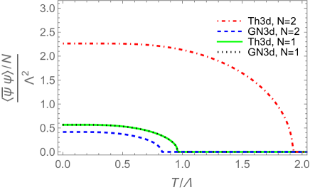
Figure 2: The chiral condensate as a function of $T$ for $\mu=0$, when $N=1$ and $N=2$.

From Fig. 2, we can also see that as $N$ decreases, the fermion condensate grows for the GN model, while for the Thirring model it moves in the opposite direction, up to $N=1$, when both condensates finally merge.

VI.3 The $T=0$ and $\mu\neq 0$ case

From Eq. (13), the effective potential for the Thirring model in the limit $T\to 0$ is given by

$$\frac{V_{\rm eff}^{\text{Th}}\left(\eta,{\overline{v}}_{0},\mu,T=0\right)}{N}=\frac{\overline{v}_{0}^{2}\Lambda}{2\pi}-\frac{2\eta^{3}}{3\pi}+\frac{3\eta^{4}}{8\pi N\Lambda}$$

$$-\left\{\frac{1}{2\pi}\left[\frac{(|\eta|-|\mu|)^{2}}{3}(2|\eta|+|\mu|)-2|\eta|^{3}+2\eta^{2}|\mu|\right.\right.$$

$$\left.\left.-\overline{v}_{0}\left(\mu^{2}-\eta^{2}\right)\right]\right.$$

$$\left.+\frac{1}{32\pi N\Lambda}\left[13\eta^{4}-14\eta^{2}\mu^{2}+\mu^{4}\right]\right\}\theta(|\mu|-|\eta|).$$

In this case, the zeroth component of the auxiliary vector field is given by

$$\overline{v}_{0}=-\frac{\mu^{2}-\eta^{2}}{2\Lambda}\theta(|\mu|-|\eta|).$$ (53)

At the same time, the GN effective potential, from Eq.  (14) in the $T=0$ limit, reads

$$\frac{V_{\rm eff}^{\rm GN}\left(\eta,{\overline{\sigma}},\mu,T=0\right)}{N} =-\frac{{\overline{\sigma}}^{2}\Lambda}{2\pi}-\frac{2|\eta|^{3}}{3\pi}+\frac{{\overline{\sigma}}\eta^{2}}{\pi}-\frac{\eta^{4}}{8\pi N\Lambda}$$ (54)

$$\quad-\Bigg{\{}\frac{1}{2\pi}\left[\frac{(|\eta|-|\mu|)^{2}}{3}(2|\eta|+|\mu|)+2\eta\left(\eta-{\overline{\sigma}}\right)(|\mu|-|\eta|)\right]$$

$$\quad+\frac{1}{32\pi N\Lambda}\left[4\eta^{2}\left(\mu^{2}-\eta^{2}\right)+\left(\eta^{2}-\mu^{2}\right)^{2}\right]\Bigg{\}}\theta(|\mu|-|\eta|)\,,$$

where

$${\overline{\sigma}}=\frac{\eta^{2}}{\Lambda}+\frac{\eta}{\Lambda}(|\mu|-|\eta|)\theta(|\mu|-|\eta|)\,.$$ (55)

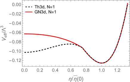
Figure 3: The effective potential as a function of $\eta$ for $T=0$ and $\mu=\Lambda$, with $N=1$. The variational mass is normalized by $\bar{\eta}(0)$, which represents the optimal value in vacuum (broken) phase, $\bar{\eta}(0)=4\Lambda/3$.

As it is well known, at large-$N$ the GN model suffers a chiral first-order phase transition when the two phases (symmetric and broken) coexist at the (coexistence) chemical potential $\mu_{\text{c}}=\Lambda$. Going beyond the large-$N$ approximation, it has been shown that the value of $\mu_{\text{c}}$ increases as $N$ decreases Kneur:2007vj ; Kneur:2007vm . To review how $\mu_{\text{c}}$ can be determined, let us examine both effective potentials. In Fig. 3 we show this quantity for each model, at $N=1$, as a function of the variational masses for the emblematic (GN large-$N$) value $\mu_{c}=\Lambda$. The figure illustrates part of a typical first-order transition pattern. At this chemical potential value the global (stable) minima for both models lies at ${\overline{\eta}}_{\text{GN}}={\overline{\eta}}_{\text{Th}}\equiv{\overline{\eta}}(0)$, where ${\overline{\eta}}(0)=4\Lambda/3$ represents the optimal variational mass corresponding to the vacuum (broken) phase for the relevant $N=1$ case (see Eqs. (34) and (36)). The dynamics of the first-order phase transition can then be understood by observing how the effective potential extremum, at ${\overline{\eta}}_{\text{GN}}={\overline{\eta}}_{\text{Th}}\equiv 0$, behave as $\mu\to\mu_{\text{c}}$. When $\mu=0$, $V_{\rm eff}$ is characterized by a maximum at the origin and then, as $\mu$ further increases, this maximum becomes an inflection point signaling the first spinodal. At even higher $\mu$ values the inflection becomes a local (metastable) minimum, as Fig. 3 suggests. As discussed in Refs. Kneur:2007vj ; Kneur:2007vm for the GN case, the phase transition happens when the minima at the origin and at ${\overline{\eta}}(0)$ become degenerate. In this case, the chemical potential value at which the broken (vacuum) and symmetric (compressed) matter coexist can be determined from $V_{\rm eff}(\overline{\eta}(0),\mu_{\text{c}})=V_{\rm eff}(\overline{\eta}=0,\mu_{\text{c}})$. Recalling that $V_{\rm eff}(\overline{\eta})=\Omega$ one can determine $\mu_{\text{c}}$ in the Thirring case by equating Eq. (35) to

$$\begin{split}\Omega_{\text{Th}}\left(\overline{\eta}=0,\overline{v}_{0},\mu,T=0\right)&=\frac{\overline{v}_{0}^{2}\Lambda}{2\pi}-\frac{\overline{v}_{0}\mu^{2}}{2\pi}-\frac{|\mu|^{3}}{6\pi}-\frac{\mu^{4}}{32\pi N\Lambda}\\ &=-\frac{|\mu|^{3}}{6\pi}\left[1+\left(1+\frac{1}{4N}\right)\frac{3|\mu|}{4\Lambda}\right]\,,\end{split}$$ (56)

obtaining

$$\big{|}\mu_{\text{c}}^{\text{(Th)}}\big{|}=\frac{4\Lambda N}{3}\left[1+\left(1+\frac{1}{4N}\right)\frac{3}{4\Lambda}\big{|}\mu_{\text{c}}^{\text{(Th)}}\big{|}\right]^{-1/3}\,.$$ (57)

Adopting the same strategy in the GN case, one must equate Eq. (37) to

$$\Omega_{\text{GN}}\left(\overline{\eta}=0,\overline{\sigma}=0,\mu,T=0\right)=-\frac{|\mu|^{3}}{6\pi}\left(1+\frac{3}{16N}\frac{\left|\mu\right|}{\Lambda}\right)\,,$$ (58)

which gives the result

$$\big{|}\mu_{\text{c}}^{\text{(GN)}}\big{|}=\frac{\Lambda}{1-\frac{1}{4N}}\left(1+\frac{3}{16N}\frac{\big{|}\mu_{\text{c}}^{\text{(GN)}}\big{|}}{\Lambda}\right)^{-1/3}\,,$$ (59)

and which confirms the well established large-$N$ result, $\mu_{c}=\Lambda$, when $N\to\infty$  Rosenstein:1990nm . Then, defining $\Delta\left|\mu_{\text{c}}\right|=\big{|}\mu_{\text{c}}^{\text{(Th)}}\big{|}-\big{|}\mu_{\text{c}}^{\text{(GN)}}\big{|}$ , allows us to write

$$\Delta\left|\mu_{\text{c}}\right| =\frac{4\Lambda N}{3}\left\{\frac{1}{\left[1+\left(1+\frac{1}{4N}\right)\frac{3}{4\Lambda}\big{|}\mu_{\text{c}}^{\text{(Th)}}\big{|}\right]^{1/3}}\right.$$

$$\quad\left.-\frac{3}{\left(4N-1\right)\left(1+\frac{3}{16\Lambda N}\big{|}\mu_{\text{c}}^{\text{(GN)}}\big{|}\right)^{1/3}}\right\}.$$ (60)

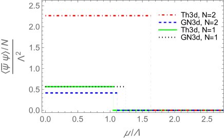
Figure 4: The fermion condensate as function of $\mu$ for $T=0$ when $N=1$ and $N=2$.

As one could anticipate from Fig. 4, which shows the chiral fermion condensate for both the GN and Thirring models as a function of the chemical potential the two models do not predict an equivalent result for $\mu_{\text{c}}$ even when $N=1$, at least in the first order in the OPT scheme, since

$$\Delta\left|\mu_{\text{c}}\right| =\frac{4\Lambda}{3}\left[\left(1+\frac{15}{16\Lambda}\big{|}\mu_{\text{c}}^{\text{(Th)}}\big{|}\right)^{-1/3}\right.$$

$$\quad\left.-\left(1+\frac{3}{16\Lambda}\big{|}\mu_{\text{c}}^{\text{(GN)}}\big{|}\right)^{-1/3}\right]\,.$$ (61)

Indeed, for $N=1$, an explicit evaluation gives $\big{|}\mu_{\text{c}}^{\text{(Th)}}\big{|}=1.05946\Lambda$ and $\big{|}\mu_{\text{c}}^{\text{(GN)}}\big{|}1.24337\Lambda$, such that $\Delta\left|\mu_{\text{c}}\right|=0.18391\Lambda$, as Eq. (61) predicts. To further understand the origin of such discrepancy, we can now check the equivalence of the thermodynamic potentials at the two degenerate minima, starting with the one which represents the broken (vacuum) phase. In this case, Eqs. (35) and (37) explicitly show that both thermodynamic potentials exactly coincide at ${\overline{\eta}}(0)$, in agreement with the result shown in Fig. 3. On the other hand, the difference between the thermodynamic potentials at the origin as given by Eqs. (56) and (58) gives the following non-vanishing result

$$\frac{\Delta\Omega({\overline{\eta}}=0,\mu,T=0)}{N}\Bigg{|}_{N=1}=-\frac{\mu^{4}}{8\pi\Lambda}=-\frac{\overline{v}_{0}(\overline{\eta}_{\text{Th}}=0)^{2}\Lambda}{2\pi}\,,$$ (62)

which, precisely agrees with Eq. (5) upon setting $\eta=0$ in the latter. From Eq. (62), we can confirm that, as observed in Sec. IV, the agreement between the GN and the Thirring models does not hold at finite densities. This difference is a result of the vector field expectation value contribution to the Thirring model, which does not seem to have a counterpart within the GN model, at least at the approximation level adopted here. In this context, it is worth recalling that the OPT (radiatively) generates a vector-like contribution to the GN model through the two-loop term proportional to $(\delta\lambda/N)\mathcal{W}_{p}^{2}$  Kneur:2012qp ; Restrepo:2014fna . However, this term is not sufficient to compensate the similar type of contributions arising within the Thirring model at $N=1$.

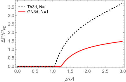
Figure 5: The normalized pressure difference for the Thirring and GN models at $N=1$ and $T=0$ as function of the chemical potential. $P_{FD}=\mu^{3}/(6\pi)$ is the free Fermi-Dirac gas pressure for massless fermions.

As a consequence of the discussion given above, the observed discrepancy also manifests itself in other thermodynamic quantities as the chemical potential increases. As an example, in Fig. 5 we show the pressure for both models at $N=1$ and $T=0$ as a function of the chemical potential. In this figure, where the pressure is normalized by the pressure of the free Fermi-Dirac gas of massless fermions, $P_{FD}=\mu^{3}/(6\pi)$, one can see how the pressure difference rises with increasing values of $\mu$.

VI.4 The $T\neq 0$ and $\mu\neq 0$ case

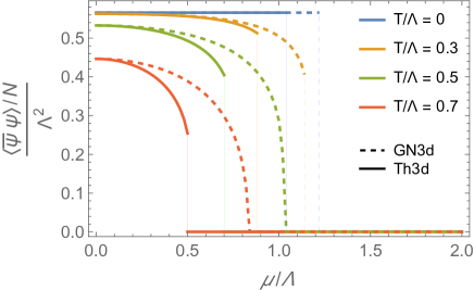
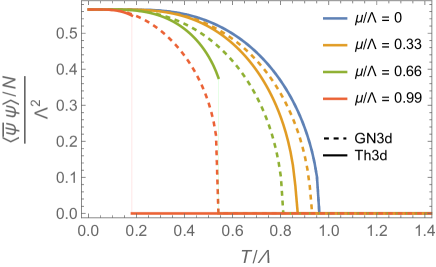
Figure 6: The fermion condensate for the Thirring and GN models at $N=1$, as a function of the chemical potential, for fixed values of the temperature (panel a) and as a function of the temperature, for fixed values of the chemical potential (panel b).

For completeness and illustration purposes, let us also (numerically) study the case relevant for a hot and dense system of fermions starting with Fig. 6 which displays the fermion condensates, as a function of $\mu$, for fixed values of the temperature (panel a) and as a function of the temperature, for fixed values of $\mu$ (panel b). Note that as the chemical potential increases, the discrepancy between each model increases, as expected from all the previous discussions.

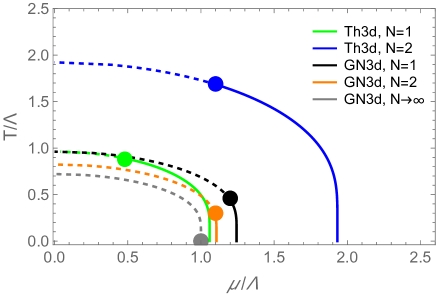
Figure 7: The phase diagram for the GN and Thirring models for different values of $N$. The dashed lines represent a second-order transition boundary, while the solid lines represent the first-order transition boundary. The dots represent the tricritical points separating the two different types of transitions.

Finally, in Fig. 7 we show the phase diagram, on the $T-\mu$ plane, for each model at some representative values of $N$. Once again, it is instructive to observe the behavior of each transition boundary as the value of $N$ decreases towards the value $N=1$. As $N$ decreases, the chiral symmetry broken region for the Thirring model shrinks, while for the GN model it expands and they seem to converge to each other. At $N=1$ they approximately agree to each other at lower values of the chemical potential, but eventually one overshoots the other as $\mu$ increases. In particular, the tricritical points representing each model are quite separated, even at $N=1$.

VII Conclusions

In this paper, we have analyzed the duality between the Thirring and Gross-Neveu models in $2+1$-dimensions in order to explicitly confirm that they are equivalent when $N=1$, in accordance with the predictions from the Fierz identities. As both models are typically studied in the large-$N$ approximation, which is simply not reliable enough to study the predicted equivalence in the case of a single flavor, here we have made use of the optimized perturbation theory approximation which can easily incorporate $1/N$ contributions.

For our purposes, the OPT capability to generate corrections going beyond the simple (mean-field) large-$N$ predictions already at the first non trivial order is of particular interest, since it offers a unique twofold opportunity: gauge the method’s reliability and check the predicted equivalence between the two models. Considering the two distinct effective potentials, at first perturbative order, we have then compared the resulting phase transition patterns at finite $N$ values. As far as the duality regime at $N=1$ is concerned, we have demonstrated that it indeed holds whenever the density vanishes. In such cases, the OPT at its first nontrivial order has shown to be already quite appropriate. At finite values of $\mu$, however, the equivalence of both models for $N=1$ could not be fully confirmed, at least at the approximation level considered here. Yet, the approximation was sufficient to show that as $N$ decreases from large-$N$ values toward $N=1$, both models display opposing behaviors regarding the chiral phase transition. While the chiral symmetry breaking region increases for the GN model as $N$ decreases, the Thirring model displays an opposite behavior, with the chiral symmetry breaking region collapsing. In particular, the critical temperatures for chiral symmetry restoration satisfy $T_{c}^{(\rm GN)}<T_{c}^{(\rm Thirring)}$ for $N>1$ and $T_{c}^{(\rm GN)}=T_{c}^{(\rm Thirring)}$ at $N=1$. For the coexistence chemical potentials we also have a similar behavior, with $\mu_{c}^{(\rm GN)}<\mu_{c}^{(\rm Thirring)}$ when $N>1$, but eventually, at $N=1$, one overshoots the other. We have traced the latter unexpected discrepancy as a consequence of the presence of a non-vanishing vacuum expectation value associated with the auxiliary vector field present in the Thirring model. While it is known that the OPT approximation can radiatively generate vector contributions already at its first perturbative order Kneur:2012qp ; Restrepo:2014fna , here we have observed that such ($1/N$) contributions to the GN model, proportional to $(\lambda/N)\mathcal{W}_{p}^{2}\sim(\lambda/N)\langle\psi^{\dagger}\psi\rangle^{2}$, are not enough to fully compensate all the terms proportional to $\mathcal{W}_{p}^{2}$ in the Thirring model (which include $N^{0}$ and $1/N$ powers).

In future works it becomes of interest to investigate whether, by pushing the OPT approximation to higher orders, the differences observed here at finite chemical potentials will eventually cancel, leading to the expected equivalence when $N=1$. It would also be useful to explore other nonperturbative methods, capable to go beyond the large-$N$ approximation, to study this same problem. In summary, the predicted equivalence between the Thirring and Gross-Neveu models at $N=1$ seems to offer a distinctive opportunity to test different nonperturbative methods and to gauge their reliability by providing an appropriate, and rather simple, platform. Finally, we remark that this first OPT application to the planar Thirring model predicts that the critical flavor number preventing chiral symmetry breaking for this model is $N=\infty$, in agreement with the Gaussian approximation results Hyun:1994fb .

Appendix A Dirac matrices trace properties in $2+1$ Dimensions

The following expressions involve traces of products of Dirac matrices in $2+1$ dimensions and which are found in the computation of the effective potentials:

$$\begin{gathered}\operatorname{Tr}\left[(\eta-\not{v})(\not{p}+\eta)\right]=4\left(\eta^{2}-p\cdot v\right),\\ \operatorname{Tr}\left[(\not{p}+\eta)\gamma_{\mu}(\not{q}+\eta)\gamma^{\mu}\right]=4\left(3\eta^{2}-p\cdot q\right).\end{gathered}$$ (63)

The $\gamma^{\mu}$ matrices in $2+1$ dimensions are defined as

$$\gamma^{\mu}=\left(\begin{array}[]{cc}1&0\\ 0&-1\end{array}\right)\otimes\sigma^{\mu}=\left(\begin{array}[]{cc}\sigma^{\mu}&0\\ 0&-\sigma^{\mu}\end{array}\right),$$ (64)

with $\sigma^{\mu}=\left(\sigma^{3},i\sigma^{x},i\sigma^{y}\right)$, and $\bar{\psi}=\psi^{\dagger}\gamma^{0}$ is the adjoint spinor. The $\gamma^{\mu}$ matrices satisfy the Clifford algebra $\left\{\gamma^{\mu},\gamma^{\nu}\right\}=2\eta^{\mu\nu}\mathbbm{1}$. They also obey the identity

$$\gamma^{\mu}\gamma^{\nu}=g^{\mu\nu}\mathbbm{1}+i\epsilon^{\mu\nu\lambda}\gamma_{3}\gamma_{\lambda},$$ (65)

where $\mathbbm{1}=\mathbbm{1}_{4\times 4}$, $\gamma_{3}=\left(\begin{array}[]{cc}\mathbbm{1}_{2\times 2}&0\\ 0&-\mathbbm{1}_{2\times 2}\end{array}\right)$.

The non-trivial traces involving these $\gamma^{\mu}$ matrices are given by

$$\operatorname{Tr}\left(\gamma^{\mu}\gamma^{\nu}\right) =4g^{\mu\nu},$$ (66)

$$\operatorname{Tr}\left(\gamma^{\mu}\gamma^{\nu}\gamma^{\lambda}\gamma_{3}\right) =4i\epsilon^{\mu\nu\lambda},$$

$$\operatorname{Tr}\left(\gamma^{\mu}\gamma^{\nu}\gamma^{\alpha}\gamma^{\beta}\right) =4\left(g^{\mu\nu}g^{\alpha\beta}+g^{\mu\alpha}g^{\nu\beta}-g^{\mu\beta}g^{\nu\alpha}\right).$$

The Dirac matrices also satisfy the following identities,

$$\gamma_{\mu}\gamma^{\mu} =3\mathbbm{1},\quad\gamma^{\mu}\gamma_{\nu}\gamma_{\mu}=-\gamma_{\nu},$$ (67)

$$\gamma^{\mu}\gamma_{\nu}\gamma_{\lambda}\gamma_{\mu} =3g_{\nu\lambda}\mathbbm{1}-i\epsilon_{\nu\lambda\kappa}\gamma^{\kappa}\gamma_{3},$$

$$\epsilon^{\mu\nu\kappa}\gamma_{\mu}\gamma_{\nu} =-2i\gamma^{\kappa}\gamma_{3},$$

$$\epsilon^{\mu\nu\kappa}\gamma_{\mu}\not{a}\gamma_{\nu} =-2ia^{\kappa}\gamma_{3}.$$

Appendix B Momentum integrals and Matsubara’s sums

The integrals in Feynman diagrams at finite temperature and density use the substitution $p_{0}\rightarrow i\left(\omega_{n}-i\mu\right)=(2n-1)i\pi T+\mu$, where $\mu$ is the chemical potential and $\omega_{n}=(2n+1)\pi T$ are the Matsubara frequencies for fermions, with $n\in\mathbbm{Z}$:

$$\int\frac{d^{d}p}{(2\pi)^{d}}f\left(p_{0},|\mathbf{p}|\right)$$

$$\rightarrow iT\sum_{n=-\infty}^{+\infty}\int\frac{d^{d-1}\mathbf{p}}{(2\pi)^{d-1}}f\left[i\left(\omega_{n}-i\mu\right),|\mathbf{p}|\right].$$ (68)

Defining the dispersion relation

$$E^{2}_{\mathbf{p}}=\mathbf{p}^{2}+\eta^{2}\,,$$ (69)

one can perform the relevant thermal integrals as follows. Starting with

$$\mathcal{X}_{p}(\eta) = i\int\frac{d^{d}p}{(2\pi)^{d}}\ln\left(p^{2}-\eta^{2}\right)$$

$$= -T\sum_{n=-\infty}^{+\infty}\int\frac{d^{d-1}\mathbf{p}}{(2\pi)^{d-1}}\ln\left[\left(\omega_{n}-i\mu\right)^{2}+E^{2}_{\mathbf{p}}\right],$$

and upon using the Matsubara sum relation one obtains

$$T\sum_{n=-\infty}^{+\infty}\ln\left[\left(\omega_{n}-i\mu\right)^{2}+E^{2}_{\mathbf{p}}\right]=E_{\mathbf{p}}$$

$$+T\ln\left[1+e^{-(E_{\mathbf{p}}+\mu)/T}\right]$$

$$+T\ln\left[1+e^{-(E_{\mathbf{p}}-\mu)/T}\right].$$ (71)

Then, performing the momentum integration within the $\overline{\rm MS}$ regularization scheme one obtains

$$\mathcal{X}_{p}(\eta) = \frac{|\eta|^{3}}{6\pi}+\frac{\eta}{2\pi}T^{2}\left\{\operatorname{Li}_{2}\left[-e^{-(|\eta|-|\mu|)/T}\right]\right.$$

$$+ \left.\operatorname{Li}_{2}\left[-e^{-(|\eta|+|\mu|)/T}\right]\right\}$$

$$+ \frac{T^{3}}{2\pi}\left\{\operatorname{Li}_{3}\left[-e^{-(|\eta|-|\mu|)/T}\right]\right.$$

$$+ \left.\operatorname{Li}_{3}\left[-e^{-(|\eta|+|\mu|)/T}\right]\right\}.$$

Next, let us consider the integral

$$\mathcal{Y}_{p}(\eta) = i\int\frac{d^{d}p}{(2\pi)^{d}}\frac{1}{p^{2}-\eta^{2}}$$ (73)

$$= T\sum_{n=-\infty}^{+\infty}\int\frac{d^{d-1}\mathbf{p}}{(2\pi)^{d-1}}\frac{1}{\left(\omega_{n}-i\mu\right)^{2}+E_{\mathbf{p}}^{2}}.$$

In this case, the Matsubara sum reads

$$T\sum_{n=-\infty}^{+\infty}\frac{1}{\left(\omega_{n}-i\mu\right)^{2}+E_{\mathbf{p}}^{2}}$$

$$=\frac{1}{2E_{\mathbf{p}}}\left[1-\frac{1}{e^{(E_{\mathbf{p}}+\mu)/T}+1}-\frac{1}{e^{(E_{\mathbf{p}}-\mu)/T}+1}\right]\;,$$

and performing the momentum integration, one obtains

$$\mathcal{Y}_{p}(\eta) = -\frac{T}{4\pi}\left\{\frac{|\eta|}{T}\right.$$

$$+ \left.\ln\left[1+e^{-(|\eta|-|\mu|)/T}\right]+\ln\left[1+e^{-(|\eta|+|\mu|)/T}\right]\right\}.$$

Finally, let us consider

$$\mathcal{W}_{p}(\eta) = i\int\frac{d^{d}p}{(2\pi)^{d}}\frac{p_{0}}{p^{2}-\eta^{2}}$$

$$= iT\sum_{n=-\infty}^{+\infty}\int\frac{d^{d-1}p}{(2\pi)^{d-1}}\frac{\left(\omega_{n}-i\mu\right)}{\left(\omega_{n}-i\mu\right)^{2}+E_{\mathbf{p}}^{2}},$$

and the Matsubara sum relation

$$T\sum_{n=-\infty}^{+\infty}\frac{\left(\omega_{n}-i\mu\right)}{\left(\omega_{n}-i\mu\right)^{2}+E_{\mathbf{p}}^{2}}$$ (77)

$$= \frac{i}{2}\left[\frac{1}{1+e^{\left(E_{\mathbf{p}}-\mu\right)/T}}-\frac{1}{1+e^{\left(E_{\mathbf{p}}+\mu\right)/T}}\right],$$

which, after integrating over $\mathbf{p}$ gives

$$\mathcal{W}_{p}(\eta) = -\operatorname{sgn}(\mu)\frac{T^{2}}{4\pi}\left\{\frac{|\eta|}{T}\ln\left[\frac{1+e^{(|\eta|+|\mu|)/T}}{1+e^{(|\eta|-|\mu|)/T}}\right]\right.$$

$$+ \left.\operatorname{Li}_{2}\left[-e^{(|\eta|+|\mu|)/T}\right]-\operatorname{Li}_{2}\left[-e^{(|\eta|-|\mu|)/T}\right]\right\},$$

which only contributes at finite densities ($\mu\neq 0$).

It is useful also to quote the $T\to 0$ limit of the above functions,

$$\mathcal{X}_{p}(\eta)\Bigr{|}_{T\to 0} = \frac{|\eta|^{3}}{6\pi}-\frac{\eta}{4\pi}(|\mu|-|\eta|)^{2}\theta(|\mu|-|\eta|)$$ (79)

$$+ \frac{1}{12\pi}(|\eta|-|\mu|)^{3}\theta(|\mu|-|\eta|),$$

$$\mathcal{Y}_{p}(\eta)\Bigr{|}_{T\to 0} = -\frac{|\eta|}{4\pi}-\frac{1}{4\pi}(|\mu|-|\eta|)\theta(|\mu|-|\eta|),$$

$$\mathcal{W}_{p}(\eta)\Bigr{|}_{T\to 0} = -\frac{1}{8\pi}\operatorname{sgn}(\mu)\left(\mu^{2}-\eta^{2}\right)\theta(|\mu|-|\eta|).$$

References

- (1) Y. Nambu and G. Jona-Lasinio, Dynamical Model of Elementary Particles Based on an Analogy with Superconductivity. I., Phys. Rev. 122, 345-358 (1961) doi:10.1103/PhysRev.122.345
- (2) Y. Nambu and G. Jona-Lasinio, Dynamical model of elementary particles based on an analogy with superconductivity. II., Phys. Rev. 124, 246-254 (1961) doi:10.1103/PhysRev.124.246
- (3) D. J. Gross and A. Neveu, Dynamical Symmetry Breaking in Asymptotically Free Field Theories, Phys. Rev. D 10, 3235 (1974) doi:10.1103/PhysRevD.10.3235
- (4) W. E. Thirring, A Soluble Relativistic Field Theory?, Annals Phys. 3, 91 (1958) doi:10.1016/0003-4916(58)90015-0
- (5) S. Hands and C. Strouthos, Quantum Critical Behaviour in a Graphene-like Model, Phys. Rev. B 78, 165423 (2008) doi:10.1103/PhysRevB.78.165423 [arXiv:0806.4877 [cond-mat.str-el]].
- (6) D. Ebert, K. G. Klimenko, P. B. Kolmakov and V. C. Zhukovsky, Phase Transitions in Hexagonal, Graphene-Like Lattice Sheets and Nanotubes Under the Influence of External Conditions, Annals Phys. 371, 254 (2016) doi:10.1016/j.aop.2016.05.001 [arXiv:1509.08093 [cond-mat.mes-hall]].
- (7) D. Ebert and D. Blaschke, Thermodynamics of a Generalized Graphene-Motivated (2+1) D Gross–Neveu Model Beyond the Mean Field Within the Beth–Uhlenbeck Approach, PTEP 2019, 123I01 (2019) doi:10.1093/ptep/ptz110 [arXiv:1811.07109 [cond-mat.mes-hall]].
- (8) V. C. Zhukovsky, K. G. Klimenko and T. G. Khunjua, Superconductivity in Chiral-Asymmetric Matter within the (2+1)-Dimensional Four-Fermion Model, Moscow Univ. Phys. Bull. 72, 250 (2017) doi:10.3103/S002713491703016X
- (9) K. G. Klimenko, R. N. Zhokhov and V. C. Zhukovsky, Superconductivity Phenomenon Induced by External In-Plane Magnetic Field in (2+1)-Dimensional Gross-Neveu Type Model, Mod. Phys. Lett. A 28, 1350096 (2013) doi:10.1142/S021773231350096X [arXiv:1211.0148 [hep-th]].
- (10) Y. M. P. Gomes and R. O. Ramos, Tilted Dirac Cone Effects and Chiral Symmetry Breaking in a Planar Four-Fermion Model, Phys. Rev. B 104, 245111 (2021) doi:10.1103/PhysRevB.104.245111 [arXiv:2106.09239 [cond-mat.mes-hall]].
- (11) Y. M. P. Gomes and R. O. Ramos, Superconducting Phase Transition in Planar Fermionic Models with Dirac Cone Tilting, Phys. Rev. B 107, 125120 (2023) doi:10.1103/PhysRevB.107.125120 [arXiv:2204.08534 [cond-mat.str-el]].
- (12) Y. M. P. Gomes, E. Martins, M. B. Pinto and R. O. Ramos, First-Order Phase Transitions within Weyl Type of Materials at Low Temperatures, Phys. Rev. B 108, 085107 (2023) doi:10.1103/PhysRevB.108.085107 [arXiv:2305.09007 [cond-mat.str-el]].
- (13) H. Caldas, J. L. Kneur, M. B. Pinto and R. O. Ramos, Critical Dopant Concentration in Polyacetylene and Phase Diagram from a Continuous Four-Fermi model, Phys. Rev. B 77, 205109 (2008) doi:10.1103/PhysRevB.77.205109 [arXiv:0804.2675 [cond-mat.soft]].
- (14) H. Caldas and R. O. Ramos, Magnetization of Planar Four-Fermion Systems, Phys. Rev. B 80, 115428 (2009) doi:10.1103/PhysRevB.80.115428 [arXiv:0907.0723 [cond-mat.soft]].
- (15) R. O. Ramos and P. H. A. Manso, Chiral Phase Transition in a Planar Four-Fermi Model in a Tilted Magnetic Field, Phys. Rev. D 87, 125014 (2013) doi:10.1103/PhysRevD.87.125014 [arXiv:1303.5463 [hep-ph]].
- (16) K. G. Klimenko and R. N. Zhokhov, Magnetic Catalysis Effect in the (2+1)-Dimensional Gross-Neveu Model With Zeeman Interaction, Phys. Rev. D 88, 105015 (2013) doi:10.1103/PhysRevD.88.105015 [arXiv:1307.7265 [hep-ph]].
- (17) T. G. Khunjua, K. G. Klimenko and R. N. Zhokhov, Spontaneous Non-Hermiticity in the (2+1)-dimensional Gross-Neveu Model, Phys. Rev. D 105, 025014 (2022) doi:10.1103/PhysRevD.105.025014 [arXiv:2112.13012 [hep-th]].
- (18) M. M. Gubaeva, T. G. Khunjua, K. G. Klimenko and R. N. Zhokhov, Spontaneous Non-Hermiticity in the (2+1)-Dimensional Thirring Model, Phys. Rev. D 106, 125010 (2022) doi:10.1103/PhysRevD.106.125010 [arXiv:2212.01062 [hep-th]].
- (19) T. G. Khunjua, K. G. Klimenko and R. N. Zhokhov, Hartree-Fock Approach to Dynamical Mass Generation in the Generalized (2+1)-Dimensional Thirring Model, Phys. Rev. D 106, 085002 (2022) doi:10.1103/PhysRevD.106.085002 [arXiv:2208.11735 [hep-th]].
- (20) M. Fierz, Zur Fermischen Theorie des -Zerfalls, Z. Phys. 104, 553 (1937) doi:10.1007/bf01330070
- (21) J. F. Nieves and P. B. Pal, Generalized Fierz Identities, Am. J. Phys. 72, 1100 (2004) doi:10.1119/1.1757445 [arXiv:hep-ph/0306087 [hep-ph]].
- (22) B. Rosenstein and A. Kovner, Gross-Neveu and Thirring Models. Covariant Gaussian Analysis, Phys. Rev. D 40, 523 (1989) doi:10.1103/PhysRevD.40.523
- (23) A. W. Wipf and J. J. Lenz, Symmetries of Thirring Models on 3D Lattices, Symmetry 14, 333 (2022) doi:10.3390/sym14020333 [arXiv:2201.01692 [hep-lat]].
- (24) F. Karsch, Lattice QCD at High Temperature and Density, Lect. Notes Phys. 583, 209 (2002) doi:10.1007/3-540-45792-5_6 [arXiv:hep-lat/0106019 [hep-lat]].
- (25) S. Muroya, A. Nakamura, C. Nonaka and T. Takaishi, Lattice QCD at Finite Density: An Introductory Review, Prog. Theor. Phys. 110, 615 (2003) doi:10.1143/PTP.110.615 [arXiv:hep-lat/0306031 [hep-lat]].
- (26) A. Okopinska, Nonstandard Expansion Techniques for the Effective Potential in Quantum Field Theory, Phys. Rev. D 35, 1835 (1987) doi:10.1103/PhysRevD.35.1835
- (27) A. Duncan and M. Moshe, Nonperturbative Physics from Interpolating Actions, Phys. Lett. B 215, 352 (1988) doi:10.1016/0370-2693(88)91447-5
- (28) V. I. Yukalov, Interplay between Approximation Theory and Renormalization Group, Phys. Part. Nucl. 50, 141 (2019) doi:10.1134/S1063779619020047 [arXiv:2105.12176 [hep-th]].
- (29) J. L. Kneur, M. B. Pinto, R. O. Ramos and E. Staudt, Updating the Phase Diagram of the Gross-Neveu Model in 2+1 Dimensions, Phys. Lett. B 657, 136 (2007) doi:10.1016/j.physletb.2007.10.013 [arXiv:0705.0673 [hep-ph]].
- (30) J. L. Kneur, M. B. Pinto, R. O. Ramos and E. Staudt, Emergence of Tricritical Point and Liquid-Gas Phase in the Massless 2+1 Dimensional Gross-Neveu Model, Phys. Rev. D 76, 045020 (2007) doi:10.1103/PhysRevD.76.045020 [arXiv:0705.0676 [hep-th]].
- (31) J. L. Kneur, M. B. Pinto and R. O. Ramos, Thermodynamics and Phase Structure of the Two-Flavor Nambu–Jona-Lasinio Model Beyond Large-, Phys. Rev. C 81, 065205 (2010) doi:10.1103/PhysRevC.81.065205 [arXiv:1004.3815 [hep-ph]].
- (32) J. L. Kneur, M. B. Pinto and R. O. Ramos, Phase Diagram of the Magnetized Planar Gross-Neveu Model Beyond the Large- Approximation, Phys. Rev. D 88, 045005 (2013) doi:10.1103/PhysRevD.88.045005 [arXiv:1306.2933 [hep-ph]].
- (33) M. B. Pinto and R. O. Ramos, High Temperature Resummation in the Linear Delta Expansion, Phys. Rev. D 60, 105005 (1999) doi:10.1103/PhysRevD.60.105005 [arXiv:hep-ph/9903353 [hep-ph]].
- (34) M. B. Pinto and R. O. Ramos, A Nonperturbative Study of Inverse Symmetry Breaking at High Temperatures, Phys. Rev. D 61, 125016 (2000) doi:10.1103/PhysRevD.61.125016 [arXiv:hep-ph/9912273 [hep-ph]].
- (35) R. L. S. Farias, G. Krein and R. O. Ramos, Applicability of the Linear Delta Expansion for the Field Theory at Finite Temperature in the Symmetric and Broken Phases, Phys. Rev. D 78, 065046 (2008) doi:10.1103/PhysRevD.78.065046 [arXiv:0809.1449 [hep-ph]].
- (36) D. S. Rosa, R. L. S. Farias and R. O. Ramos, Reliability of the Optimized Perturbation Theory in the 0-Dimensional Scalar Field Model, Physica A 464, 11 (2016) doi:10.1016/j.physa.2016.07.067 [arXiv:1604.00537 [hep-ph]].
- (37) R. L. S. Farias, R. O. Ramos and D. S. Rosa, Symmetry Breaking Patterns for Two Coupled Complex Scalar Fields at Finite Temperature and in an External Magnetic Field, Phys. Rev. D 104, 096011 (2021) doi:10.1103/PhysRevD.104.096011 [arXiv:2109.03671 [hep-ph]].
- (38) P. M. Stevenson, Optimized Perturbation Theory, Phys. Rev. D 23, 2916 (1981) doi:10.1103/PhysRevD.23.2916.
- (39) J. L. Kneur, M. B. Pinto and R. O. Ramos, Critical and Tricritical Points for the Massless 2D Gross-Neveu Model Beyond Large , Phys. Rev. D 74, 125020 (2006) doi:10.1103/PhysRevD.74.125020 [arXiv:hep-th/0610201 [hep-th]].
- (40) S. K. Gandhi, H. F. Jones and M. B. Pinto, The Delta Expansion in the Large Limit, Nucl. Phys. B 359, 429 (1991) doi:10.1016/0550-3213(91)90067-8.
- (41) S. Hyun, G. H. Lee and J. H. Yee, Gaussian Approximation of the (2+1)-Dimensional Thirring Model in the Functional Schrodinger Picture, Phys. Rev. D 50, 6542 (1994) doi:10.1103/PhysRevD.50.6542 [arXiv:hep-th/9406070 [hep-th]].
- (42) B. Rosenstein, B. Warr and S. H. Park, Dynamical Symmetry Breaking in Four Fermi Interaction Models, Phys. Rept. 205, 59 (1991) doi:10.1016/0370-1573(91)90129-A.
- (43) J. L. Kneur, M. B. Pinto, R. O. Ramos and E. Staudt, Vector-Like Contributions from Optimized Perturbation in the Abelian Nambu–Jona-Lasinio Model for Cold and Dense Quark Matter, Int. J. Mod. Phys. E 21, 1250017 (2012) doi:10.1142/S0218301312500176 [arXiv:1201.2860 [nucl-th]].
- (44) T. E. Restrepo, J. C. Macias, M. B. Pinto and G. N. Ferrari, Dynamical Generation of a Repulsive Vector Contribution to the Quark Pressure, Phys. Rev. D 91, 065017 (2015) doi:10.1103/PhysRevD.91.065017 [arXiv:1412.3074 [hep-ph]].