11email: nbsi@space.dtu.dk 22institutetext: DTU Space, Technical University of Denmark, Elektrovej 327, DK-2800 Kgs. Lyngby, Denmark
22email: shuji@dtu.dk 33institutetext: Niels Bohr Institute, University of Copenhagen, Jagtvej 128, DK-2200 Copenhagen, Denmark 44institutetext: AIM, CEA, CNRS, Université Paris-Saclay, Université Paris Diderot, Sorbonne Paris Cité, F-91191 Gif-sur-Yvette, France 55institutetext: School of Astronomy and Space Science, Nanjing University, Nanjing 210093, China
55email: taowang@nju.edu.cn 66institutetext: Key Laboratory of Modern Astronomy and Astrophysics (Nanjing University), Ministry of Education, Nanjing 210093, China 77institutetext: IRAM,300 rue de la piscine, F-38406 Saint-Martin d’Hères, France 88institutetext: Purple Mountain Observatory, Chinese Academy of Sciences, 10 Yuanhua Road, Nanjing 210023, China 99institutetext: Instituto de Astrofísica de Canarias, C. Vía Láctea, s/n, 38205 La Laguna, Tenerife, Spain 1010institutetext: Universidad de La Laguna, Dpto. Astrofísica, 38206 La Laguna, Tenerife, Spain 1111institutetext: Instituto de Física, Pontificia Universidad Católica de Valparaíso, Casilla 4059, Valparaíso, Chile 1212institutetext: Department of Physics & Astronomy, University of California Los Angeles, 430 Portola Plaza, Los Angeles, CA 90095, USA 1313institutetext: Max-Planck-Institut für Extraterrestrische Physik (MPE), Giessenbachstrasse 1, 85748 Garching, Germany 1414institutetext: INAF-Osservatorio Astronomico di Trieste, Via Tiepolo 11, 34131, Trieste, Italy 1515institutetext: IFPU-Institute for Fundamental Physics of the Universe, Via Beirut 2, 34014, Trieste 1616institutetext: European Southern Observatory, Karl-Schwarzschild-Str. 2, D85748 Garching bei Munchen, Germany 1717institutetext: Department of Astronomy, University of Geneva, Chemin Pegasi 51, 1290 Versoix, Switzerland 1818institutetext: Department of Astronomy, Tsinghua University, Beijing 100084, China 1919institutetext: Chinese Academy of Sciences South America Center for Astronomy (CASSACA), National Astronomical Observatories of China (NAOC), 20A Datun Road 2020institutetext: INAF- Osservatorio Astronomico di Brera, via Brera 28, I-20121, Milano, Italy & via Bianchi 46, I-23807, Merate, Italy 2121institutetext: Department of Physics, University of Helsinki, Gustaf Hällströmin katu 2, FI-00014 Helsinki, Finland 2222institutetext: School of Physics and Astronomy, Institute for Astronomy, University of Edinburgh, Royal Observatory, Blackford Hill, EH9 3HJ Edinburgh, UK 2323institutetext: Sub-Department of Astrophysics, University of Oxford, Keble Road, Oxford OX1 3RH, UK 2424institutetext: Department of Physics and Astronomy, University of the Western Cape, Robert Sobukwe Road, 7535 Bellville, Cape Town, South Africa 2525institutetext: Kavli IPMU (WPI), UTIAS, The University of Tokyo, Kashiwa, Chiba 277-8583, Japan 2626institutetext: Inter-university Institute for Data Intensive Astronomy, Department of Physics and Astronomy, University of the Western Cape, 7535 Bellville, Cape Town, South Africa
NOEMA formIng Cluster survEy (NICE): Characterizing eight massive galaxy groups at in the COSMOS field††thanks: Tables C1 to C8 are only available in electronic form at the CDS via anonymous ftp to cdsarc.u-strasbg.fr (130.79.128.5) or via http://cdsweb.u-strasbg.fr/cgi-bin/qcat?J/A+A/.
The NOrthern Extended Millimeter Array (NOEMA) formIng Cluster survEy (NICE) is a NOEMA large programme targeting 69 massive galaxy group candidates at over six deep fields with a total area of 46 deg2. Here we report the spectroscopic confirmation of eight massive galaxy groups at redshifts in the Cosmic Evolution Survey (COSMOS) field. Homogeneously selected as significant overdensities of red IRAC sources that have red Herschel colours, four groups in this sample are confirmed by CO and [CI] line detections of multiple sources with NOEMA 3mm observations, three are confirmed with Atacama Large Millimeter Array (ALMA) observations, and one is confirmed by H emission from Subaru/FMOS spectroscopy. Using rich ancillary data in the far-infrared and sub-millimetre, we constructed the integrated far-infrared spectral energy distributions for the eight groups, obtaining a total infrared star formation rate (SFR) of 260-1300 yr-1. We adopted six methods for estimating the dark matter masses of the eight groups, including stellar mass to halo mass relations, overdensity with galaxy bias, and NFW profile fitting to radial stellar mass densities. We find that the radial stellar mass densities of the eight groups are consistent with a NFW profile, supporting the idea that they are collapsed structures hosted by a single dark matter halo. The best halo mass estimates are with a general uncertainty of 0.3 dex. Based on the halo mass estimates, we derived baryonic accretion rates (BARs) of for this sample. Together with massive groups in the literature, we find a quasi-linear correlation between the integrated SFR/BAR ratio and the theoretical halo mass limit for cold streams, , with with a scatter of . Furthermore, we compared the halo masses and the stellar masses with simulations, and find that the halo masses of all structures are consistent with those of progenitors of galaxy clusters, and that the most massive central galaxies have stellar masses consistent with those of the brightest cluster galaxy progenitors in the TNG300 simulation. Above all, the results strongly suggest that these massive structures are in the process of forming massive galaxy clusters via baryonic and dark matter accretion.
Key Words.:
Galaxy: evolution – galaxies: high-redshift – submillimeter: galaxies – galaxies: clusters: general1 Introduction
Galaxy clusters are the largest virialized structures in the local Universe, and their progenitors (see Overzier, 2016, for a review) are suspected to be massive galaxy groups and protoclusters in the early Universe (Muldrew et al., 2015). At high redshifts, massive groups and protoclusters represent the earliest massive collapsed structures hosted by massive dark matter halos (Wang et al., 2016; Willis et al., 2020; Di Mascolo et al., 2023). Characterizing their dark matter halos provides key constraints on cosmological parameters that can be used to test structure formation theories (Overzier, 2016). On the other hand, the evolutionary track between the early structures and local clusters is a major topic in modern astrophysics but remains poorly understood (Chiang et al., 2013; Shimakawa et al., 2018). These early () massive structures host a large number of star-forming galaxies rich in dust and gas (e.g. Dannerbauer et al. 2014; Oteo et al. 2018; Gobat et al. 2019). The most massive members of these structures are often found to have vigorous starbursts (e.g. Oteo et al., 2018; Miller et al., 2018; Zhou et al., 2024), while some members are already quiescent at (e.g. Kubo et al., 2021; Kalita et al., 2021; McConachie et al., 2022; Ito et al., 2023; Jin et al., 2024). The diverse populations of member galaxies and their rapid evolution make them an ideal laboratory for studying the formation of clusters and brightest cluster galaxies (BCGs; Shi et al., 2024; Jin et al., 2024). Therefore, studying a large sample of galaxy groups and (proto-)clusters before cosmic noon (i.e. the peak of star formation at ; Madau & Dickinson, 2014), where groups and (proto-)clusters are expected to contribute significantly to the cosmic star formation rate (SFR) density, is essential to unveiling the evolution and formation of massive galaxies and clusters (Chiang et al., 2017).
In the last decade, massive groups and (proto-)clusters have been discovered at cosmic noon and out to the epoch of re-ionization (; e.g. Hu et al. 2021; Brinch et al. 2023; Jones et al. 2023; Arribas et al. 2023; Morishita et al. 2023) using various techniques. To date, most structures have been selected by mapping overdensity of galaxies, including the overdensities of optical/near-infrared (NIR) sources (e.g. Gobat et al., 2011; Wang et al., 2016), dusty star-forming galaxies (e.g. Dannerbauer et al., 2014), and star-forming galaxies detected in the radio (e.g. Daddi et al., 2017, 2021). However, a major limitation of the overdensity mapping is the line-of-sight projection (e.g. Chen et al., 2023). In this regard, advanced techniques that include colour and redshift information, for example red IRAC colours (Wylezalek et al., 2013, 2014; Mei et al., 2023), narrowband emitters (Koyama et al., 2013; Shimakawa et al., 2014; Hu et al., 2021), and photometric or spectroscopic redshifts (e.g. Cucciati et al., 2018; Sillassen et al., 2022; Helton et al., 2023; Jin et al., 2024), have significantly improved the efficiency and robustness of the selection. Second, far-infrared (FIR) and (sub-)millimetre-bright dusty star-forming galaxies have been used to detect high- protocluster candidates, which were later confirmed by follow-up observations, for example GN20 (Daddi et al., 2009), AzTEC3 (Capak et al., 2011), the SCUBA2-selected HDF850.1 (Walter et al., 2011), the Herschel-selected DRC (Oteo et al., 2018) and HerBS-70 (Bakx et al., 2024), and the millimetre-selected SPT2349-56 (Miller et al., 2018). Third, extended X-ray emission from hot plasma in the intracluster medium (ICM) can be used to trace mature clusters (e.g. Stanford et al., 2006). Fourth, Sunyaev-Zel’dovich (SZ) emission (Sunyaev & Zeldovich, 1970) is a sign of a collapsed massive structure, where cosmic microwave background photons are accelerated by the host ICM in clusters via inverse Compton scattering (e.g. Staniszewski et al., 2009). Finally, extended Ly emission (Ly blobs), stemming from cool gas in dense regions associated with overdensities of galaxies, can be used to trace actively star-forming massive groups (e.g. Prescott et al., 2008). A new technique that uses Ly absorption has recently been exploited to search for galaxy groups missed by other surveys: Ly tomography (Lee et al., 2018; Newman et al., 2022).
Overdensity mapping and dusty star-forming galaxy (DSFG) tracers are widely used to search for massive structures at , for which the other methods are either infeasible (e.g. SZ and X-ray) or require prohibitively time-consuming observations. Therefore, a combined search of FIR-luminous objects and overdensities of optical/NIR galaxies provides an efficient and powerful tool for selecting massive galaxy groups and protoclusters. However, this method still suffers from projection effects, and high quality photometric redshifts are required to associate the FIR emission with the candidate overdensities. Recently, the advent of deep, wide, and panchromatic extragalactic survey fields, such as the Cosmic Evolution Survey (COSMOS), and the construction of state-of-the-art, multi-band photometric catalogues (e.g. COSMOS2020; Weaver et al. 2022) have made this cluster selection method more viable than ever before. The efficiency of this combined search method has been verified by some pilot projects; they successfully selected the cluster CLJ1001, which was later spectroscopically confirmed to reside at (Wang et al., 2016), as well as three massive groups at (Daddi et al., 2021, 2022b). These discoveries demonstrated the potential of building large, homogeneously selected samples of massive groups and protoclusters in large and deep survey fields.
The dark matter halo mass is a vital parameter of these identified groups and protoclusters, and an accurate estimate of halo masses is crucial to assessing their dynamical and evolutionary states (Chiang et al., 2013; Ata et al., 2022; Montenegro-Taborda et al., 2023). To date, various methods have been exploited to estimate the dark matter halo mass of galaxies and galaxy groups, including (1) the stellar-to-halo mass relation (SHMR; e.g. Behroozi et al., 2013; Shuntov et al., 2022), (2) dynamical constraints of member galaxies (e.g. Wang et al., 2016; Miller et al., 2018), (3) X-ray emission from the hot ICM (e.g. Gobat et al., 2011; Wang et al., 2016), and (4) the SZ effect from the inverse Compton scattering of cosmic microwave background photons (e.g. Gobat et al., 2019; Di Mascolo et al., 2023). However, constraining the dark matter halo mass of structures in the early Universe remains a challenging task. This is because (1) optical data are often too shallow to allow for accurate stellar mass measurements (Daddi et al., 2021), (2) spectroscopic surveys of high- structures are too incomplete for membership identification, (3) X-ray observations from current facilities are not deep enough to probe the hot ICM (Overzier, 2016), and (4) the SZ effect is a powerful tool but one that is very demanding in terms of observing time, and only a couple of structures have been detected at (Gobat et al., 2019; Di Mascolo et al., 2023). Recently, Wang et al. (2016) found that the stellar mass density profile of the X-ray-detected cluster CLJ1001 can be fitted by a projected Navarro-Frenk-White (NFW) profile (Navarro, Frenk, & White, 1997), suggesting that the structure is virialized and that the halo has a relatively high concentration (Sun et al., 2024). The similar shape of the two profiles implies that the halo mass can be estimated from the stellar mass density profile, which provides an efficient and powerful approach to constraining the halo mass of collapsed structures. However, this novel method has yet to be tested with a statistically robust sample at high redshifts and still suffers from limitations (1) and (2).
Another open question concerns the growth of galaxies residing in massive structures. Theoretically, structures with dark matter halo masses above would generate shocks and heat the infalling gas of the intergalactic medium to the temperature of the ICM (Birnboim & Dekel, 2003), preventing further star formation and the growth of cluster galaxies. However, advanced simulations predict a mechanism of gas inflow in which cold streams travelling along intersections of dense filaments are able to penetrate the halo without being shock-heated (Dekel & Birnboim, 2006; Dekel et al., 2009; Rosdahl & Blaizot, 2012; Mandelker et al., 2020). This regime of cold gas inflow in a hot environment is defined by a redshift-dependent theoretical upper limit of the host halo mass where these streams can efficiently occur, , and a theoretical lower limit of the host halo mass where shock heating occurs, (Dekel et al., 2013). Nevertheless, observational evidence for this picture is lacking. The model from Goerdt et al. (2010) predicted that this mode of cold accretion would be detectable via collision-driven Ly emission. This idea is supported by the recent discovery of giant Ly nebulae in massive galaxy groups at by Daddi et al. (2021, 2022b). The rate of accretion of both cold and warm gas can be quantified with the baryonic accretion rate (BAR), which is predicted to scale with the dark matter halo mass (Goerdt et al., 2010) and the total SFR it feeds (Daddi et al., 2022b). To further verify and observationally constrain this picture of cold accretion, a large sample of homogeneously selected massive galaxy groups and protoclusters is needed.
Finally, the fate of massive structures in the early Universe remains unresolved. Whether massive groups of galaxies at high- will form present-day clusters, a proposition that is fundamental for precisely defining the term ‘protocluster’, remains an open question. Currently, there are no direct observables that can offer a robust characterization and accurate classification of protoclusters (Overzier, 2016). Instead, comparisons between the observables and cosmological simulations provide a feasible approach to inferring the evolutionary stage and final fate of structures (e.g. Chiang et al., 2013; Miller et al., 2018; Ata et al., 2022; Jin et al., 2023, 2024).
In this paper we report spectroscopic confirmation of eight galaxy groups from the NOrthern Extended Millimeter Array (NOEMA) formIng Cluster survEy (NICE) in the COSMOS field and study their integrated stellar, gas, dust, and dark matter properties. The paper is organized as follows: We describe the sample and selection in Section 2. In Section 3 we describe the observations and data reduction. In Section 4 we explain in detail our analysis methods. We present our results in Section 5, discuss the corresponding science in Section 6, and summarize this study in Section 7. We adopt a flat cosmology with parameters , , and , and use a Chabrier (2003) initial mass function. Magnitudes are in the AB system (Oke, 1974).
2 NOEMA formIng Cluster survEy (NICE)
NICE is a 159 hours NOEMA large programme (ID:M21AA, PIs: E. Daddi and T. Wang) targeting 48 massive galaxy group candidates in the COSMOS, Lockman Hole, Elais-N1, Boötes, and XMM-LSS fields. This programme is complemented by a 40 hours Atacama Large submillimeter Array (ALMA) programme (ID: 2021.1.00815.S, PI: E. Daddi) targeting 25 candidates in the southern sky in the ECDFS, COSMOS, and XMM-LSS fields. Four candidates are observed with both NOEMA and ALMA. Overall, 69 targets are selected in a total of 46 deg2 sky area. The first discovery of NICE is a star-bursting group in the Lockman Hole field, which was recently reported in Zhou et al. (2024). In this paper, we focus on the eight candidates in the COSMOS field (Table 1), of which four are observed with NOEMA, three are observed with ALMA, and one is observed with both facilities.
In Table 1 we list the eight massive galaxy group candidates of this study: seven of them (i.e. COS-SBC3, COS-SBC4, COS-SBC6, COS-SBCX1, COS-SBCX3, COS-SBCX4, and COS-SBCX7) were selected as a significant overdensity of red IRAC sources with red Herschel colours, following the identical selection method utilized by Zhou et al. (2024). The selection is described in detail in Zhou et al. (2024), and we briefly list the selection criteria below:
(1) Overdensity of red IRAC sources:
| (1) | ||||
where [3.6] and [4.5] are IRAC channel 1 and 2 magnitudes from the COSMOS2020 catalogue (Weaver et al., 2022). We used the distance to the -th nearest neighbour to quantify the local galaxy density, and constructed a galaxy surface density map of . We selected overdensities with either or that are above the field levels in log scale (e.g. Wang et al. 2016).
(2) Herschel detection with red colours:
| (2) | ||||
Additionally, the target HPC1001 was originally selected by Sillassen et al. (2022) using the overdensity of COSMOS2020 sources at and an overdensity of ALMA sources. We note that HPC1001 has red IRAC colours as in Eq. 1 but was not selected as an IRAC overdensity. This is because HPC1001 is extremely compact, and the members are severely blended in the low-resolution IRAC images. However, the of sources in HPC1001 is 6.8 above the average, which is one of the strongest overdensities in the COSMOS field at (Sillassen et al., 2022). Furthermore, HPC1001 satisfies the criteria of Herschel selection (Eq. 2) and shows even redder colours. Therefore, the eight candidates share a consistent selection, constituting a homogeneous sample. Benefiting from the rich multi-wavelength datasets and well-established catalogues in the COSMOS field, the eight high- group candidates are entitled to the best data quality in the NICE sample, constituting an ideal sample for this initial statistical study of the NICE programme.
| Target name | RA | Dec. | Programme ID | Sensitivitya | Beam | Ancillary ID | Sens.b | Ang. Res.c | |
| [deg] | [deg] | [mJy/beam] | [arcsec] | [mJy/beam] | [arcsec] | ||||
| (NOEMA) | |||||||||
| HPC1001 | 150.4656 | 2.6359 | M21AA | 2013.1.00034.S | 0.06 | 0.4 | |||
| COS-SBCX3 | 150.3113 | 2.4511 | M21AA | 2016.1.00463.S | 0.26 | 0.8 | |||
| COS-SBCX4 | 150.7509 | 2.4132 | M21AA | 2016.1.00463.S | 0.27 | 0.8 | |||
| COS-SBCX7 | 149.9898 | 1.7978 | M21AA | 2015.1.00137.S | 0.12 | 1.0 | |||
| (ALMA) | |||||||||
| COS-SBC3 | 150.7196 | 2.6995 | 2021.1.00815.S | 2021.1.00246.S | 0.02 | 1.6 | |||
| COS-SBC6 | 149.7057 | 2.2160 | 2021.1.00815.S | 2016.1.00463.S | 0.27 | 0.8 | |||
| COS-SBC4 | 150.0364 | 2.2177 | 2021.1.00815.S | 2016.1.00463.S | 0.27 | 0.8 | |||
| (NOEMA + ALMA) | |||||||||
| COS-SBCX1 | 150.3492 | 2.7619 | M21AA | 0.14 | 2016.1.00463.S | 0.26 | 0.8 | ||
| 2021.1.00815.S |
Notes: aline sensitivity over . bThe redshift is measured from Subaru/FMOS observations (Kashino et al., 2019). bContinuum sensitivity of the ancillary ALMA data. cAngular resolution of the ancillary ALMA data.
3 Data
The eight galaxy group candidates in the COSMOS field are observed with the NOEMA and ALMA interferometers. A summary of our observations is provided in Table 1, and we describe them in detail below.
3.1 NOEMA
As a part of the NICE large programme, five targets were observed with NOEMA (Table 1). The observations were designed with two frequency setups of two sidebands each in NOEMA Band 1, covering CO(3-2) and CO(4-3) in the redshift ranges and , respectively. The first setup covered the frequencies of the most probable CO lines. If lines were detected with the first setup, the second setup was not executed. The observations were conducted in October 2022 with a total on-source time of 10.8h for the five targets in track sharing mode with array configurations C and D. The data were reduced and calibrated using the institut de radioastronomie millimétrique (IRAM) software package111https://www.iram.fr/IRAMFR/GILDAS. The final data products were generated in uv tables, reaching an average continuum sensitivity of and line sensitivity over a 500 km s-1 line width at 100 GHz, with an average angular resolution of (see details in Table 1).
3.2 ALMA
ALMA Band 4 and 5 observations of four targets were carried out in Cycle 8. We designed four frequency tunings that cover one or multiple CO and CI lines based on the estimated redshift of the groups. The four tunings cover the frequency range , but leave two gaps at 157.5–168.5 GHz and 170–178 GHz. The observations were conducted in August 2022, reaching an rms sensitivity of over a 500 km s-1 line width at GHz. The raw data were reduced and calibrated using the Common Astronomy Software Application (CASA; McMullin et al. 2007) pipeline. Following our standard pipeline (e.g. Coogan et al. 2018; Jin et al. 2019, 2022; Zhou et al. 2024), we converted the calibrated measurement sets to uvfits format for further analysis with the GILDAS/mapping software. In each ALMA tuning, we achieved an average continuum sensitivity of and an angular resolution of .
3.3 Spectrum extraction pipeline
The extraction of NOEMA and ALMA spectra is carried out with the pipeline adopted in Zhou et al. (2024). Briefly, we extracted spectra in the space (visibility) using the uvfit routine of GILDAS. The uvfit run was performed on the original uv tables at all frequencies, where we adopted a point source model for the sources, using prior positions from the COSMOS2020 catalogue or ALMA continuum images. To enhance the sensitivity in overlapping frequency ranges, we combined all spectral windows of ALMA into a single 1D spectrum for each source.
3.4 Ancillary data
We utilized the rich multi-wavelength data and catalogues in the COSMOS field. In the optical and NIR, we adopted the COSMOS2020 photometric catalogue (Weaver et al., 2022), along with the provided photometric redshifts and stellar masses that were crucial for the identification of spectral lines in our data and for characterization of the physical properties of the member galaxies. At FIR and sub-millimetre wavelengths, we made use of the MIPS 24 m (Le Floc’h et al., 2009), Herschel 100–500 m (Lutz et al., 2011), SCUBA-2 850 m (Simpson et al., 2019), and AzTEC 1.1 mm maps (Aretxaga et al., 2011), and we measured the integrated fluxes of this sample by performing the super-deblending technique (Liu et al., 2018b; Jin et al., 2018). For radio bands, we used the low-resolution MeerKAT-DR1 image with a beam size of and frequency range 1.15–1.35 GHz (Jarvis et al. 2016; Heywood et al. 2022; Hale et al. in prep.). We also used the archival ALMA data (ID: 2016.1.00463.S, PI: Y. Matsuda; ID: 2021.1.00246.S, PI: C. Chen; ID: 2015.1.00137.S, PI: N. Scoville; 2013.1.00034.S, PI: N. Scoville) for the dust continuum imaging in Band 6 and 7, and ALMA photometry from the A3COSMOS catalogue (Liu et al., 2019) where available.
4 Methodology
In this section we describe the methods adopted to determine the redshifts and group membership, as well as the integrated FIR properties, the BAR, and the halo mass of the groups.
4.1 Line detection and redshift determination
Following Zhou et al. (2024), we ran a line-searching algorithm as in Coogan et al. (2019) and Jin et al. (2019) to search for the highest integrated signal-to-noise ratio (S/N) emission lines in the 1D NOEMA/ALMA spectra. We fit the line-free continuum emission as a power-law with a fixed slope of 3.7 in frequency, assuming modified blackbody emission with (Magdis et al., 2012), by masking out channels where significant (, Jin et al. 2019) emission lines are detected. The continuum-subtracted spectra are then fitted with a Gaussian line-profile using MPFIT222http://cow.physics.wisc.edu/~craigm/idl/idl.html, at the frequencies identified by the line searching algorithm. The redshift can be robustly identified if two or more lines are detected on one source. For sources only detected with a single line, we determined their redshifts by comparing them to the photo-z redshift probability density function (PDF(z)) from the COSMOS2020 catalogue. As an example, in Fig. 23, we determined the best solution by comparing all possible redshift solutions for each object with optical/NIR photometric PDF(z) from the Classic LePhare version of COSMOS2020. For galaxies with a broad PDF(z) and an emission line detection close to the frequency of the structure as determined by other secure members, it is assumed that its redshift is closest to the redshift of the structure. Such cases only occur on two sources (HPC1001 ID1272853 and SBCX4 ID1049929), and one of them (ID1272853) has been recently confirmed with our ALMA [CI] observation (ID: 2023.1.00652.S, PI: N. Sillassen), which further validates our identification method.
4.2 Candidate member selection
With the photometric redshifts in the COSMOS2020 catalogue (Weaver et al., 2022), we selected candidate group members with within the virial projected radius from the group centres (see Table 4), where is the spectroscopic redshift of the central galaxy. This redshift range is defined by the representative uncertainty at the faint end of the COSMOS2020 catalogue of (Weaver et al., 2022). The virial radius limit ensures that we were only probing the inner region of these structures. We note there is a radial- and stellar-mass-dependent expected interloper fraction (Fig. 32-right); that is, low stellar mass candidate members far from the centre have a higher chance of being interlopers. We discuss implications of interlopers in detail in Section 6.4.
4.3 Integrated FIR spectral energy distributions
A deblended FIR catalogue of the COSMOS field is publicly available (Jin et al., 2018); however, it is not directly applicable for individual galaxies in crowded group and protocluster environments. Due to the overdense nature and the large Herschel and SCUBA2 beams (15–36′′), in the group centre tens of galaxies can be present in one beam, which leads to severe blending of sources. Given the high compactness of the eight groups, we applied the super-deblending technique (Jin et al., 2018; Liu et al., 2018a) with improved priors to measure the integrated fluxes in Herschel and SCUBA2 images, following the same method applied in Daddi et al. (2021) and Zhou et al. (2024).
In detail, for each group, we defined one prior at the peak position of the SCUBA2 850 m detection (Simpson et al., 2019) to represent the whole structure. In the prior list, we excluded sources within a radius of the prior to reduce the crowding (Liu et al., 2018a). Then we subtracted faint foreground and background sources by convolving the point spread function (PSF) of each instrument to the corresponding image, and ran PSF fitting on the fixed prior positions together with other sources from COSMOS2020 that are beyond the radius of the group centre. We note that nearly all ALMA and NOEMA continuum sources in the groups are spectroscopically confirmed to be group members; hence, the contamination of dusty interlopers is negligible, and the fitting is straightforward. The PSF fitting is performed for Herschel 100-500m, SCUBA2 850m, and MeerKAT images, and the measured fluxes and their uncertainties are then calibrated by Monte Carlo simulations performed on the maps (see Jin et al. 2018 for details). Finally, we checked the residual images and find that a few groups are resolved in the MeerKAT map (beam size ); hence, we adopted aperture photometry for these. Due to its relatively high resolution (6′′), the MIPS 24m image cannot be fit with a single PSF. We thus adopted the total weighted 24m photometry of individual members in the Jin et al. (2018) catalogue. The resultant photometry is summarized in Table 15.
To infer the integrated physical properties of these groups, we fit the integrated FIR spectral energy distribution (SED) using STARDUST (Kokorev et al., 2021) with the above FIR photometry, as well as the integrated ALMA and NOEMA continuum fluxes where available. The fitting was performed at the spectroscopic redshift of each group (Table 1). Only photometric points with a significant detection () were considered in the fitting, and the rest were treated as upper limits (Kokorev et al., 2021). We note that the radio photometry is not included in the fitting. Instead, we extrapolated a radio component based on the IR luminosity using the stellar mass-dependent IR-radio relation from Delvecchio et al. (2021), assuming the average stellar mass of spectroscopically confirmed ALMA continuum-detected sources. This allows us to identify potential radio excess by comparing the IR-derived radio model with the measured radio flux.
4.4 Estimate of dark matter halo mass
Based on literature studies (e.g. Wang et al., 2016; Daddi et al., 2021, 2022b; Sillassen et al., 2022), we adopted and developed in total six methods for estimating the dark matter halo mass333We use as a shorthand to refer to the n-th method for halo mass estimation.. Our six methods are split into three main techniques; the first three methods employ the simple SHMR with the peak stellar mass and the total stellar mass, respectively, the fourth method employs overdensity with clustering bias, and the final two use projected stellar mass surface density profile fitting. We briefly summarize the six halo mass methods in Table 2, and refer the details as follows:
| Method | Input | SHMR | SMF | Overdensity | NFW fit | Assumption |
| (Stellar mass scaling with SHMR) | ||||||
| Behroozi et al. 2013 | – | – | – | – | ||
| Shuntov et al. 2022 | Muzzin et al. 2013 | – | – | Virialization | ||
| van der Burg et al. 2014 | Muzzin et al. 2013 | – | – | Virialization | ||
| (Galaxy overdensity-based) | ||||||
| – | – | – | This work | – | Virialization | |
| ( surface density profile fitting) | ||||||
| – | – | – | This work | NFW profile | ||
| – | – | – | This work | NFW profile & fixed | ||
(1) We derived a halo mass by scaling the stellar mass of the most massive central group member with the SHMR in Behroozi et al. (2013);
(2a) Following the methodology in Daddi et al. (2021, 2022b) and Sillassen et al. (2022), we computed the mass-complete total stellar mass of members within the radius . selected from mass-complete COSMOS2020 (Weaver et al., 2022), where the expected contamination from the background is (e.g. Fig. 32-left). We then extrapolated the mass down to assuming the field stellar mass function (SMF) from Muzzin et al. (2013). We subtracted the contamination of the background from the recovered total mass. This background-corrected total stellar mass was then scaled to the redshift-dependent central and satellite stellar mass () SHMR in the COSMOS2020 catalogue from Shuntov et al. (2022). This recovered halo mass was corrected for the measuring stellar mass within a radius smaller than virial, by assuming a NFW density profile (Navarro, Frenk, & White, 1997).
(2b) Using the total stellar mass in , we derived a halo mass by scaling the total stellar mass with the SHMR of clusters from van der Burg et al. (2014).
(3) We estimated halo mass based on the overdensity of the groups above the field level, following the methodology presented in Sillassen et al. (2022). A stellar mass cut, selected where the interloper fraction at the virial radius of the group was (e.g. Fig. 32-right), was applied to the entire catalogue. First, we measured the average number density of the photo-z-selected galaxies () in the mass cut COSMOS2020 Classic LePhare catalogue, and obtained the group core density by measuring the number density within the virial radius centred on the core. The depth difference between the field and the group selection was accounted for by assuming a group velocity dispersion , which is the velocity dispersion of a virialized group with at (Ferragamo et al., 2021). We then calculated the mass of a sphere with comoving virial radius , defined as the radius within which the average density is 200 times the critical density of the universe with initial halo mass from :
| (3) |
Here is the overdensity and is the average matter density at , where is the critical density of the universe at , is the Hubble parameter at , is the Hubble parameter at , and are the fraction of matter and vacuum energy of the total energy in the Universe, respectively, and is a clustering bias calculated with the Tinker et al. (2010) formalism. Using the halo mass from as an initial guess on the halo mass, we recalculated the bias in an iterative fashion from the result of this method until convergence.
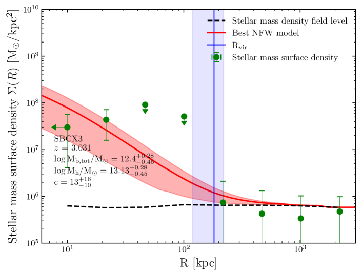
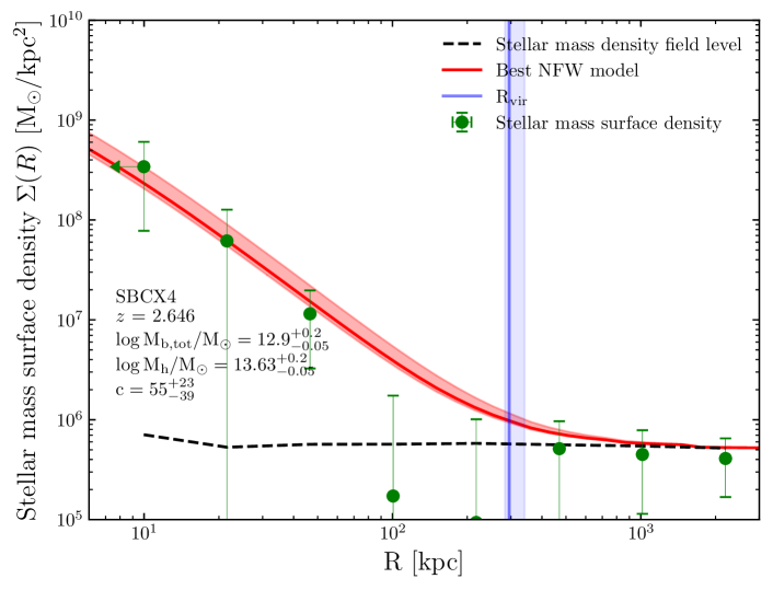
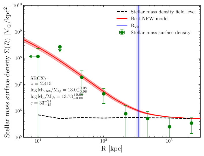
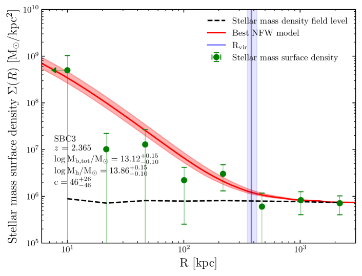
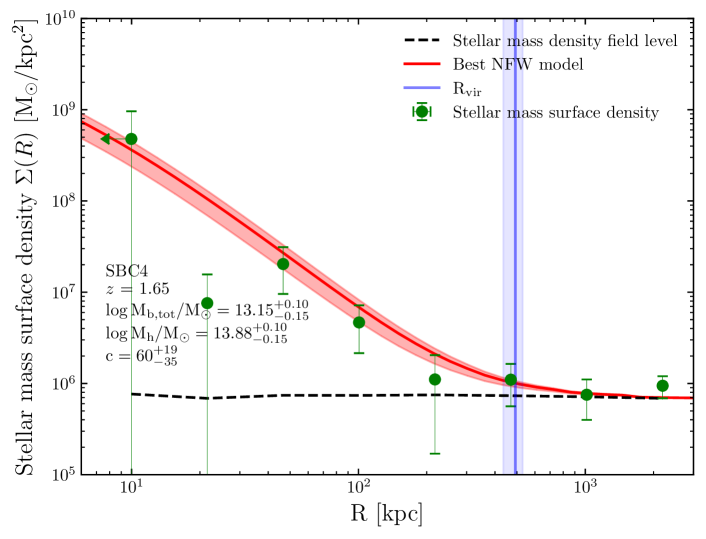
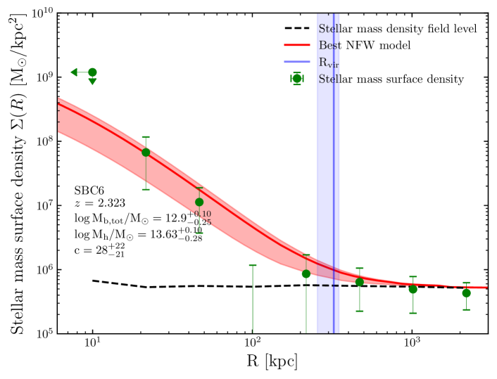
(4) Inspired by the stellar mass density profile of the X-ray detected cluster CLJ1001 being consistent with a NFW profile (Wang et al., 2016), we explored fitting the projected stellar mass density of each group using a NFW dark matter halo profile (Navarro, Frenk, & White, 1997). We assumed that the structures are virialized, their stellar mass density profiles can be described by a NFW profile, and the stellar mass profile follows the underlying dark matter profile. We first sampled the projected NFW profiles with a range of halo mass and concentration parameter values at a fixed redshift (see Appendix I). The radial bins are annuli with increasing radius from pkpc out to . We calculated a characteristic mass, , and background stellar mass density in each annulus, for the mass-complete -phot selected COSMOS2020 catalogue in 10000 randomly placed annuli. Combining the model and background, we estimated the expected number of galaxies in each radial bin, . The observed characteristic number in each radial bin was calculated as . We found the best model by maximizing the combined probability of finding when expecting ; where when and when assuming a Poisson distribution. The projected stellar mass surface density was calculated within the annuli (i.e. ) centred on the mass and distance to FIR peak weighted barycentre of spectroscopically confirmed member galaxies. The best-fit profile yields a total baryonic mass . We adopted a dark matter to baryonic mass ratio of from PLANCK cosmology (Planck Collaboration et al., 2020) to convert to halo mass .
(5) Assuming that the stellar mass density profiles largely follow NFW models, we further explored deriving halo mass solely based on the shape of the density profiles, independent of a scaling with stellar mass. We fit the stellar mass surface density profiles and their background levels using a NFW model with scale radius () as a variable. Unlike with , we fixed the concentration parameter, of the halos using the predictions from Ludlow et al. (2016), assuming a prior halo mass from the average of , , and . The best-fit value allowed us to obtain a virial radius . This virial radius is directly correlated with the halo mass, and hence we obtained the halo mass using the redshift-dependent relation from Goerdt et al. (2010).
5 Results
In this section we report the results of our analyses adopting the methodologies presented in Section 4. We produced colour images and spectra for confirmed and candidate members (Figs. 1, 12, 13, 14, 8, 9, 10 and 11) and multi-wavelength cutouts (Figs. 20, 21, 22, 16, 17, 18, 19 and 15). Coordinates and physical properties of confirmed and candidate members are shown in Tables C1 to C8.

5.1 Emission lines and redshifts
We detect robust (,) emission lines in seven out of the eight pointings, with no significant lines detected in COS-SBC4. To identify the lines and determine the redshift, we calculated all possible redshift solutions of CO and [CI] lines allowed by the observed frequencies, and compared them with the PDF(z) in the COSMOS2020 catalogue. As shown in Fig. 23 to 29, the best redshift solution is determined as the one that is closest to the peak of PDF(z). In cases where the group frequency is significantly offset from the peak of the PDF(z), for example ID1272853 in Fig. 23, we reject solutions closer to the peak as one or more bright lines would be covered but none are detected. In total, we identify 22 emission lines of CO(3-2), CO(4-3), CO(5-4), and [CI](1-0) for 20 sources. A summary of the detected lines is presented in Table 3. We detect a single emission line from 18 galaxies, and two sources are detected with two or more lines. For 58% (95%) of the sources, the best solution lies within the 1 (2) uncertainty of the estimates (Figs. 23, 28, 29, 24, 25, 26 and 27). The mean solution is in the PDF(z).
| Structure | ID | RA | Dec. | Line | WidthFWZI | S/N | |||
| [deg] | [deg] | [GHz] | [] | [] | |||||
| HPC1001 | – | 150.4659 | 2.6362 | 99.957 | CO(4-3) | 10.9 | ¡0.001 | ||
| HPC1001 | 1272853 | 150.4618 | 2.6294 | 100.004 | CO(4-3) | 3.9 | 0.001b | ||
| HPC1001 | 1274387 | 150.4647 | 2.6307 | 100.130 | CO(4-3) | 4.3 | 0.019b | ||
| COS-SBCX3 | 1088787 | 150.3105 | 2.4515 | 85.803 | CO(3-2) | 11.6 | ¡0.001 | ||
| COS-SBCX3 | 1088927 | 150.3117 | 2.4510 | 85.768 | CO(3-2) | 9.5 | ¡0.001 | ||
| COS-SBCX4 | 1050531 | 150.7504 | 2.4129 | 94.805 | CO(3-2) | 26.8 | ¡0.001 | ||
| COS-SBCX4 | 1049510 | 150.7512 | 2.4124 | 94.947 | CO(3-2) | 5.8 | ¡0.001 | ||
| COS-SBCX4 | 1049929 | 150.7522 | 2.4140 | 94.789 | CO(3-2) | 6.3 | ¡0.001 | ||
| COS-SBCX1 | 1408110 | 150.3480 | 2.7611 | 168.415 | CO(5-4) | 7.9 | ¡0.001 | ||
| ” | ” | ” | 143.797 | [CI](1-0) | 6.8 | ¡0.001 | |||
| ” | ” | ” | 134.686 | CO(4-3) | 6.3 | ¡0.001 | |||
| ” | ” | ” | 101.046 | CO(3-2) | 6.5 | ¡0.001 | |||
| COS-SBCX7 | 394609 | 149.9896 | 1.7977 | 101.228 | CO(3-2) | 9.1 | ¡0.001 | ||
| COS-SBCX7 | 394944 | 149.9882 | 1.7980 | 101.221 | CO(3-2) | 7.8 | ¡0.001 | ||
| COS-SBCX7 | 392257 | 149.9910 | 1.7967 | 101.247 | CO(3-2) | 6.0 | ¡0.001 | ||
| COS-SBCX7 | 392639 | 149.9816 | 1.7960 | 101.310 | CO(3-2) | 3.7 | 0.028b | ||
| COS-SBC3 | 1345246 | 150.7193 | 2.6998 | 154.812 | CO(5-4) | 13.1 | ¡0.001 | ||
| COS-SBC3 | 1340799 | 150.7226 | 2.6963 | 137.021 | CO(4-3) | 6.4 | ¡0.001 | ||
| ” | ” | ” | 146.305 | [CI](1-0) | 4.1 | 0.022b | |||
| COS-SBC6 | 835289 | 149.7053 | 2.2153 | 138.757 | CO(4-3) | 9.3 | ¡0.001 | ||
| COS-SBC6 | 839791 | 149.7053 | 2.2171 | 138.718 | CO(4-3) | 9.0 | ¡0.001 | ||
| COS-SBC6 | 838104 | 149.7074 | 2.2140 | 168.253 | CO(4-3) | 5.4 | ¡0.001 |
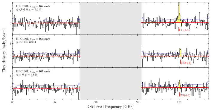
The HPC1001 is the most distant group in this sample, in which we detect three CO lines. Notably, the emission line from the core region has a velocity width of . This large width suggests a blending of multiple sources in the low resolution NOEMA beam (, Fig. 1), consistent with the fact that three ALMA 1.2 mm continuum sources are detected (at 0.4” resolution) within the NOEMA beam. As the photometric redshifts of the two i, J, and Ks-detected galaxies in the core are consistent with the CO redshift (see Fig. 23), we suspect the three galaxies to be at the same redshift . Similarly, Gómez-Guijarro et al. (2019) studied Herschel selected sources blended at similar scales, and found all blended candidate member galaxies at the same redshift, if this is also true for HPC1001, this would result in a total of five confirmed members. Our ongoing high-resolution ALMA observations (ID: 2023.1.00652.S, PI: N. Sillassen) will reveal the members in the compact core. Interestingly, we spectroscopically confirm the nearby DSFG (HPC1001.m) at (i.e. at a velocity difference of just from the core). At a projected distance of , the nearby DSFG is outside the expected virial radius of the dark matter halo (Table 4), indicating that the DSFG HPC1001.m is in a larger structure at the same redshift.
In the other groups, we can separate individual members without blending issues. We confirm two members in COS-SBCX3, three members in COS-SBCX4, four members in COS-SBCX7, one member in COS-SBC3, and two members in COS-SBC6. In the pointing COS-SBCX1, we confirmed a member with four emission lines CO(3-2), CO(4-3), [CI](1-0), and CO(5-4) all with S/N6. Though no line was detected in COS-SBC4 with ALMA, we confirm three members with Subaru/FMOS (Kashino et al., 2019). All emission lines at the redshift of COS-SBC4, , would fall out of the frequency coverage of our ALMA observations.
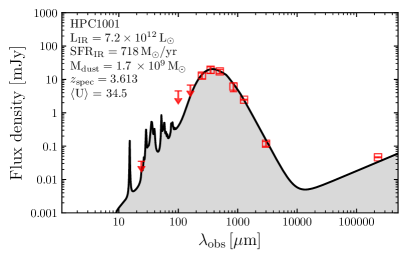
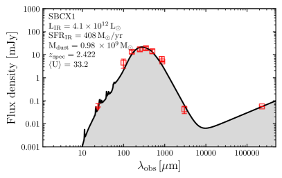
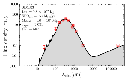
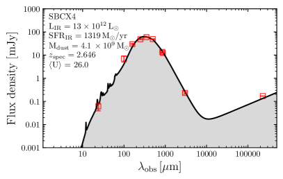
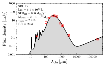
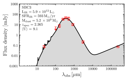
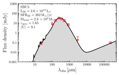
5.2 Integrated FIR properties
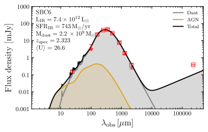
In Fig. 2 we present the best-fit of the integrated FIR photometry with STARDUST based on dust templates from Magdis et al. (2012). We obtain FIR properties of the integrated dust emission of the groups, including total IR luminosity (), SFR, dust mass () and mean radiation field (). As summarized in Table 5, we obtain integrated SFRs in the range , dust masses in the range (optically thin model), and dust-weighted mean starlight intensity scale factors in the range (Fig. 2).
Remarkably, seven of the eight FIR SEDs are well fit by pure dust emission, that is, they need no mid-IR or radio active galactic nucleus (AGN) contribution to fit the data. As shown in Fig. 2, they closely follow the IR-radio correlation with a dispersion of 0.11 dex (inter quartile range), indicating that they are powered predominantly by star formation. However, COS-SBC6 exhibits clear radio excess that suggests the presence of a radio-loud AGN. Adding a mid-IR AGN component to the fit of COS-SBC6 yields a mid-IR AGN contribution of to the total IR luminosity. We recall that the radio part of the model is not part of the fit but extrapolated using the Delvecchio et al. (2021) IR-radio correlation. By including the radio excess found in the LH-SBC3 presented in Zhou et al. (2024), this gives a radio-loud AGN fraction of 2/9 (i.e. 22%) in the NICE sample of massive galaxy groups at . This low fraction of radio-loud AGNs implies that this massive group population is primarily in star formation mode, and they are not significantly affected by AGN activity.
5.3 Dark matter halos
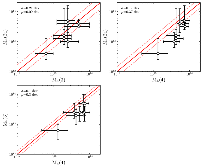
Using the methods described in Section 4.4, we estimated halo masses of as listed in Table 4. In Fig. 3 we compare , , and which represent the three main techniques of stellar mass scaling, projected galaxy overdensity, and NFW profile fitting, respectively. We calculated the standard deviation and mean offset from a 1:1 relation between each two methods (Fig. 3). We find that the results from different methods agree within 0.2–0.3 dex with systematic offsets dex, which are consistent with the expected uncertainty of lower-mass halos () at high redshifts (; Looser et al., 2021; Daddi et al., 2021, 2022b). The mean offset is in all cases , and thus with this limited sample size we are unable to detect significant systematic offsets. We adopted an average of methods , , and as the median of the best estimate, and the uncertainty is conservatively adopted as 0.3 dex, based on the scatter between methods (see Fig. 3).
| Structure | a | b | Total | (4) | Bestc | d | (5) | ||||
|---|---|---|---|---|---|---|---|---|---|---|---|
| [] | [] | [] | |||||||||
| HPC1001 | 7.7 | ||||||||||
| COS-SBCX3 | 6.0 | ||||||||||
| COS-SBCX4 | 6.0 | ||||||||||
| COS-SBCX1 | 7.0 | ||||||||||
| COS-SBCX7 | 5.6 | ||||||||||
| COS-SBC3 | 4.6 | ||||||||||
| COS-SBC6 | 4.6 | ||||||||||
| COS-SBC4 | 7.4 |
Notes: Lower limits are at significance. aPeak significance of overdensity. b is the stellar mass of the most massive central spectroscopically confirmed member galaxy. cThe best estimate halo mass is the average of , , and , and the uncertainty is estimated by the average scatter between the methods (Fig. 3). dVirial radius of Best, using the relation from Goerdt et al. (2010).
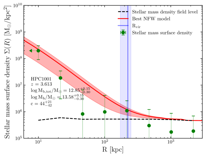
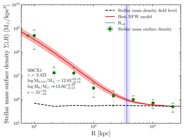
Uniquely, as shown in Fig. 4, the best fit of shows that all stellar mass density profiles can be fitted by a NFW profile. This suggests that these structures are likely already collapsed and hosted by a single dark matter halo. Furthermore, allows us to constrain the concentration parameter of the dark matter halos (see Table 16). In Fig. 31 we compare the measured concentrations with the predicted values from simulations (Ludlow et al., 2016). The comparison shows a standard deviation from the 1:1 relation of 0.28 dex, and our measured mean concentration is 0.4 dex higher than the predictions from simulations.
5.4 Baryonic accretion rate
Following the procedure in Daddi et al. (2022b) and using Eq. (5) in Goerdt et al. (2010), we estimated the total BAR:
| (4) |
Based on the best estimate of halo masses (Table 4), we calculated the BAR using Eq. 4, yielding (Table 5). The SFR arising from cold accretion can be generalized as follows:
| (5) |
where is the theoretical upper limit halo mass, where cold streams efficiently occur (Dekel & Birnboim, 2006; Daddi et al., 2022b).
Using the BAR and the fitted values of and from Daddi et al. (2022b) with Eq. 5, the expected SFR derived by the BAR are (Table 5). In six of the eight groups, the BAR-derived SFRs are consistent with our measured IR SFRs within the uncertainties, only the least massive COS-SBCX3 and the lowest redshift COS-SBC4 groups have a higher SFR than expected from the BAR. Although tentative, this rough consistency supports the baryon accretion models.
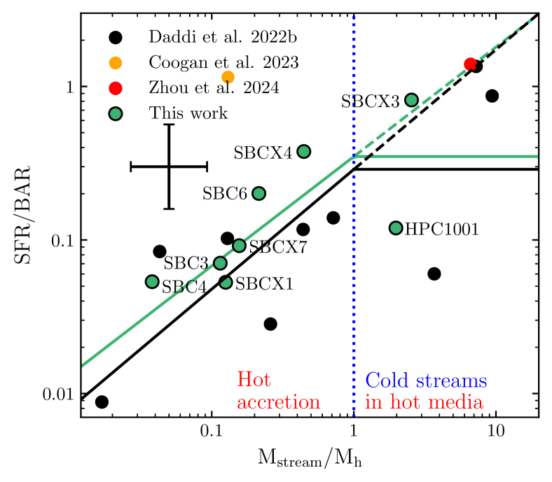
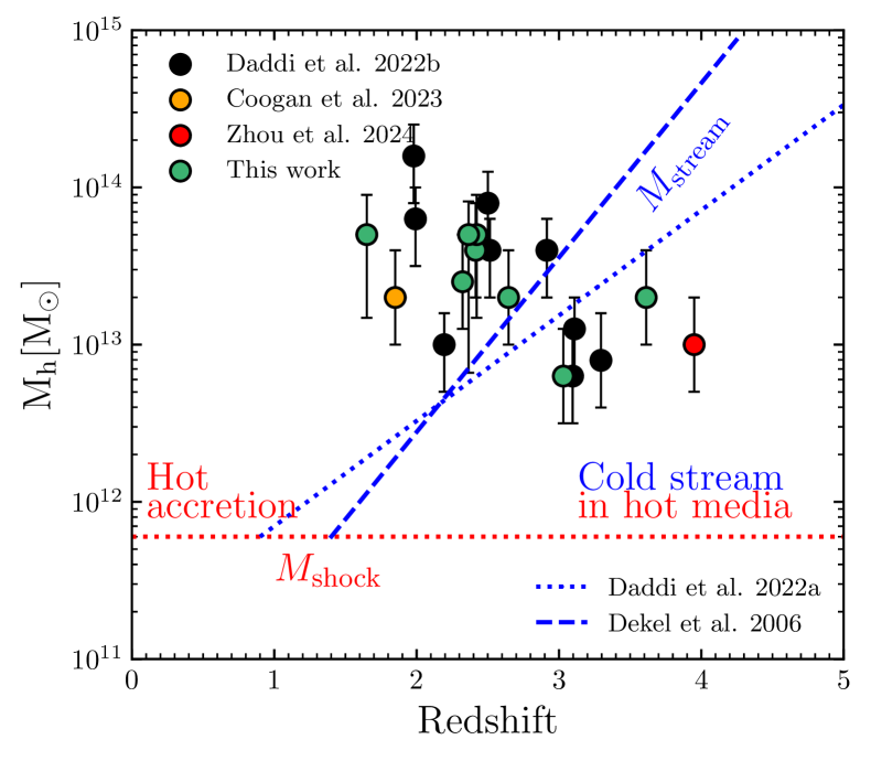
In Fig. 5 we show this sample on the diagrams of gas accretion from Daddi et al. (2022b) and Dekel et al. (2013). Interestingly, the two most distant groups, HPC1001 and COS-SBCX3, occupy the regime of cold streams in hot media, suggesting cold gas inflow. As HPC1001 has a similar halo mass to the group RO-1001 (Daddi et al., 2021), the cold streams should be detectable via Ly emission. Given that the dark matter halo estimates are prone to large uncertainties, future observations of Ly will be ideal to robustly constrain the BAR and reveal possible cold gas accretion.
As shown in Fig. 5, our sample enlarges the sample size of massive groups in Daddi et al. (2022b) by a factor of two. By including the sample in Daddi et al. (2022b) and Zhou et al. (2024), we fit a quasi-linear model to the SFR/BAR- relation, where the theoretical upper limit halo mass of cold gas streams is adopted from Eq. (2) in Daddi et al. (2022a). The best fit gives , (Fig. 5) with a scatter of assuming a linear relation, and assuming flattening at . As discussed in Coogan et al. (2023), this group in the CEERS field is a strong outlier, and we therefore excluded it from the fitting. Our fit result is in excellent agreement with the result from Daddi et al. (2022b), and is improved with better statistics. Adopting instead the definition of from (Dekel & Birnboim, 2006), does not significantly change the fitting results, but slightly increases the scatter to 0.43 dex assuming a single relation.
In the hot-accretion regime, where the estimate of is less important (Daddi et al., 2022b), we find a 0.30 dex scatter from the relation. In the cold-stream regime, we find a scatter of dex and mean offset of dex from the flattening model, and scatter of dex and mean offset of dex from the linear relation. Adopting the linear relation would result in two structures with a dex deviation from the model, where the bending model results in one dex outlier.
| Name | Best | BAR | SFRBAR | |||||
|---|---|---|---|---|---|---|---|---|
| [] | [] | [] | [] | [] | ||||
| HPC1001 | 3.613 | |||||||
| COS-SBCX3 | 3.031 | |||||||
| COS-SBCX4 | 2.646 | |||||||
| COS-SBCX1 | 2.422 | |||||||
| COS-SBCX7 | 2.415 | |||||||
| COS-SBC3 | 2.365 | |||||||
| COS-SBC6 | 2.323 | |||||||
| COS-SBC4 | 1.65 |
6 Discussion
6.1 Dark matter halo mass estimates: Prospects and caveats
Accurate estimates of halo masses are vital to inferring the evolutionary state and eventual fate of massive structures; however, it remains a challenging task especially at high redshifts. In this work, we applied three methods based on SHMR , a method based on galaxy overdensity , and developed two methods based on NFW profile fitting . Every method has its strengths and limitations, we discuss the details in the following.
is widely used in the literature (e.g. Ito et al., 2023; Brinch et al., 2024; Helton et al., 2024; Jin et al., 2024), and is solely based on the stellar mass of the most massive member galaxy. However, it is a very simplified assumption that the stellar mass of the central galaxy is solely correlated with halo mass, with a large dispersion between BCG mass and halo mass (e.g. Montenegro-Taborda et al., 2023). The accuracy of the halo mass derived with this approach can be severely affected by uncertainties in the stellar mass and redshift of the central galaxy, where the situation is even worse if the central galaxies are DSFGs, as the stellar mass estimate can be very uncertain (e.g. Long et al., 2023). Furthermore, since the relation is derived for establishing expected stellar masses given a halo mass, this results in stellar mass saturation, that is, the SHMR is almost constant at (Behroozi et al., 2013). Comparing with results from other methods, the resultant mass is inconsistent with the other methods, yielding mainly lower limits, which is rather risky when it is applied to high redshift groups. With these points in mind, we caution against the use of this method for massive galaxy groups, and massive individual galaxies.
Method scales to the total stellar mass and is clearly more advanced than . It assumes that all members are in a collapsed structure hosted by a single dark matter halo. However, it is difficult to assess whether the structure is already collapsed. The SHMR scaling is redshift dependent and has been calibrated for a high redshift (; Shuntov et al., 2022). Nevertheless, it is not calibrated to real clusters as no massive clusters exist in the COSMOS field, where this SHMR is measured. shares similar benefits and risks as . This method has been applied in several studies (e.g. Daddi et al., 2022b; Ito et al., 2023; Coogan et al., 2023). However, the scaling relation is calibrated to clusters, which might not persist, and might evolve, at higher redshift, and might not be applicable to lower-mass halos. In this work, the most massive members are all spectroscopically confirmed, and only low-mass members are identified using photometric redshifts. Although some foreground and background interlopers could be included, their low masses are not expected to significantly impact the inferred total stellar mass, and by extension the halo mass (see Section 6.4).
Unlike the above discussed methods, is not directly dependent on the stellar mass of the cluster galaxies, instead relying solely on their spatial density. A big advantage is that it is independent of uncertainties in stellar mass measurements. On the other hand, the clustering bias of the halo is not well constrained, and we simply assumed a bias value from the Tinker et al. (2010) formalism, which adds another layer of uncertainty in the estimate. Because the bias value is dependent on the halo mass, and we used the bias to calculate a halo mass, this method is circularly defined; however, we avoided this circularity by iteratively calculating the bias using as an initial guess. The bias is not 1:1 with halo mass, and the iterative approach converges quickly.
Method assumes that the stellar mass density profile traces the dark matter density profile, and that they both follow a NFW model at high redshifts. With this method, we derived a total baryonic mass and inferred a halo mass using a dark matter-to-baryon mass ratio. This assumption has been validated in low redshift clusters, for example Annunziatella et al. (2014) and Palmese et al. (2016) find both the stellar mass density and number density profiles of the clusters MACS J1206.2-0847 (Biviano et al., 2013) and RXC J2248.7-4431 can be fitted by a NFW profile, and further at cosmic noon in CLJ1449 (Strazzullo et al., 2013). Andreon (2015) find that the stellar-to-total mass ratio is radially constant in three clusters. Caminha et al. (2017) find that dark matter and hot gas asymmetry of the MACS 1206 closely follows the asymmetric distribution of the stellar component. Accordingly, if the stellar mass density profile of a high- group is found consistent with a NFW profile, it would suggest that the structure is likely collapsed. Uniquely, this method can constrain the halo mass and its concentration parameter simultaneously, which is a significant advance in characterizing dark matter halos of collapsed structures. As a proof of this method at high redshifts (), we applied it to the most distant X-ray detected cluster CLJ1001 (Wang et al., 2016, see Fig. 30). CLJ1001 is uniquely suited for this, as it is at a high redshift of and has both an X-ray and velocity dispersion calibrated halo mass. Our NFW fitting yields a halo mass of , with concentration and scale radius (Fig. 30). The recovered halo mass is in excellent agreement with the X-ray and velocity dispersion halo masses of , and, the scale radius is consistent with the one reported in Wang et al. (2016) . Nevertheless, similarly to , (2a) and (2b), this method suffers from the uncertainty on stellar masses and membership, and requires an accurate constraint on the background density level. Moreover, is also impacted by the uncertainty on the dark matter-to-baryonic mass ratio and possible inconsistency between stellar mass density profile and dark matter halo profile at high-. We also tested two methods for finding the exact centre of the group: (1) using the position of the most massive central galaxy; and (2) randomly shifting the centre position by up to a few arcseconds, instead of calculating the distance to FIR-peak-weighted barycentre. We find no significant changes in either the recovered halo masses or recovered concentrations, nor in the uncertainties of either values.
Method is a variant of . It shares with the assumption of the consistency between stellar mass density profile and halo mass density profile. However, it is totally independent of the stellar masses, as it purely relies on the shape of the profile. This is a significant advantage with respect to other methods. Notably, adopting this method with the number density profile would further reduce the bias introduced by the stellar mass estimate of the central galaxy, as the halo mass would be solely based on the distribution of member galaxies. However, this method has two major drawbacks: (1) it must assume a fixed concentration parameter to break the degeneracy between scale radius and concentration, while the fixed concentration is based on simulation results with a prior halo mass, and neither are fully tested by observations; (2) the profile fitting to the stellar mass density is dominated by the central galaxy, fitting to the number density can remove this bias but requires a larger sample of confirmed memberships. Another problem with both and is the degeneracy between , , and as they are all co-dependent and influence the shape and scaling of the density profile (Appendix I). We tried to limit this degeneracy by fixing the concentration and purely fitting the scale radius without directly incorporating the halo mass; however, this adds another layer of uncertainty as the true concentration is unknown.
Overall, the self-consistency between different methods shows encouraging prospects in halo mass estimates for high redshift structures like these. Among these methods, the NFW profile fitting and (5) are exploited for high- groups for the first time, showing potential for state-of-the-art in characterizing dark matter halos. Nevertheless, thorough analyses and tests with a large sample of low-z clusters are required to fully explore the prospects of the profile fitting techniques, and then exploit it towards high redshift, which is beyond the scope of this paper.
6.2 Nature and fate: Are these structures clusters in formation?
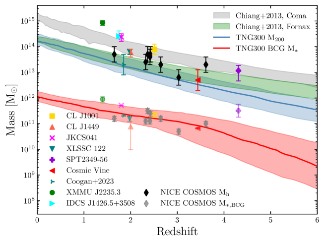
To understand the nature and fate of these structures, following Jin et al. (2024), we compared our observations with cosmological simulations. First, we compared the estimated halo masses with simulations of Coma- and Fornax-like clusters from Chiang et al. (2013). We find all groups to have halo masses consistent with progenitors of clusters with present day halo masses of at least (Fig. 6). We also compared the halo masses of this sample to clusters from the TNG300 simulation (Montenegro-Taborda et al., 2023, Fig. 6); again, we find that the halo masses of all groups are consistent with those of the progenitors of clusters (). Furthermore, we compared the stellar masses of the most massive group galaxies with that of BCG progenitors in the TNG300 simulation (Montenegro-Taborda et al., 2023), and again find they are consistent (Fig. 6). This supports the idea that the eight groups are real forming clusters, and their central galaxies are likely proto-BCGs (Jin et al., 2024).
Another approach assessing the fate of massive structures is the observationally constrained large-scale simulations, which has been recently performed by Ata et al. (2022) on the large-scale structure Hyperion (Cucciati et al., 2018). This simulation requires a highly complete spectroscopic survey of cluster members (Ata et al., 2022); hence, deep spectroscopic follow-up observations on both the cores and large-scale structure are essential. On the other hand, dedicated cluster simulations have been achieved, for example Cluster-EAGLE (Barnes et al., 2017), Magneticum (Remus et al., 2023), FLAMINGO (Schaye et al., 2023), and TNG-Cluster (Nelson et al., 2024). Further work comparing a large sample with these simulations would provide new insights into galaxy and cluster formation.
6.3 Baryonic accretion: Flattening or not?
In Fig. 5 we fit the BAR using both a quasi-linear single trend and assuming flattening at . With double sample size compared to Daddi et al. (2022b), we now find a significant () slope compared with their fit. We excluded the group from Coogan et al. (2023) as it remains a strong outlier from the expected SFR from the BAR. The group is also a strong outlier in terms of the proportions of stellar mass and SFR in the BCG, suggesting that it might be caught in a short-lived starburst connected to the formation of the BCG, or might signal a cooling flow (Coogan et al., 2023). The scatter of our fit ( dex) is somewhat lower from dex in Daddi et al. (2022b). The data do not prefer the bending model or the linear model, with nearly identical scatter of dex and dex, respectively. Instead of using the updated definition in Daddi et al. (2022a), adopting the definition from Dekel & Birnboim (2006), does not change the scatter significantly. Because the scatter in the cold-stream regime is more dependent on the halo mass (Daddi et al., 2022b), we calculated the scatters in the hot (Fig. 5-left, ) versus cold-stream (Fig. 5-left, ) regimes and find a scatter of 0.30 dex in the hot and 0.53 dex in the cold-stream regime. The expected scatter in the BAR at fixed halo mass is 0.2 dex (Correa et al., 2015), and the scatter arising from the fraction of cold gas to total gas, , is 0.1 dex (Correa et al., 2018), adding these in quadrature yields 0.3 dex in excellent agreement with our scatter in the hot regime. In the cold-stream regime, the scatter from is negligible as all accreted gas is cold, leaving a scatter from the BAR of 0.2 dex and from of 0.3 dex, adding these in quadrature yields 0.36 dex, significantly lower than the observed scatter. This increased observed scatter is only from six points and would require a larger sample to confirm; however, if real, this could indicate that there is some intrinsic stochasticity, inefficiencies in converting accreted baryonic matter into SFR, feedback mechanisms, or a combination of these processes.
6.4 Interlopers in candidate members
Given the majority of candidate members are selected with photometric redshifts, it is common that foreground and background interlopers can be included in the candidate members. We quantified the contamination of possible interlopers in two ways: (1) we measured the background number count in the mass-complete photo- selection in COSMOS2020 Classic LePhare and calculated the expected number of interlopers that can appear by chance in an aperture around the groups. We find possible mass-complete interloper fractions of () within a aperture, and the fractions increase with larger aperture, which is () within 30” (see Fig. 32-left). (2) We tested our candidate selection method in CLJ1001 (Wang et al., 2016) using the COSMOS2020 photo-z, and compare with the highly complete spectroscopic redshift sample of Sun et al. (2024). We find two clear interlopers and a total interloper fraction of in a aperture, which is largely consistent with the result of method (1). Furthermore, we also tested the interloper contamination in the total stellar mass budgets. We measured the background stellar mass in the COSMOS2020 catalogue and compared it with the total stellar mass of the groups, finding mass-complete fractions of () within and () within , respectively (see Fig. 32-right). We note that the interloper contamination were accounted for by subtracting them from the total stellar masses or overdensity when deriving halo masses.
6.5 Line-of-sight projection: Chance probabilities
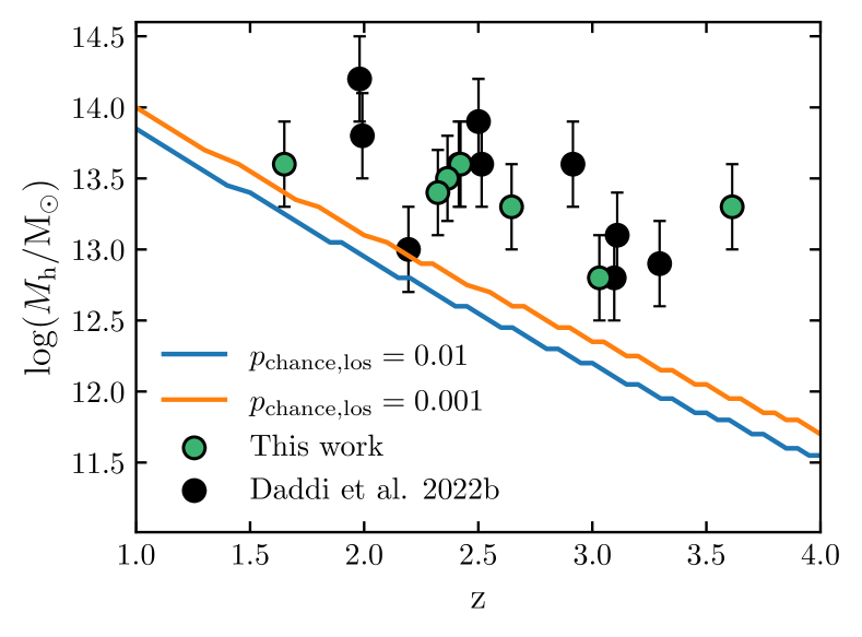
To understand the probability of finding two line-of-sight projected groups, we calculated the chance probability of finding two halos of within and indistinguishable -phot distributions (i.e. the redshift selection for halos are overlapping), using halo mass functions calculated with hmf444https://github.com/halomod/hmf (Murray et al., 2013). We multiplied this chance probability by the total number of expected halos of mass in the entire COSMOS field. The highest chance probability of this sample is the lowest redshift COS-SBC4, with , as seen in Table 6. This is only assuming the case of twin halos, and possible combinations of triples or more halos are not considered; however, this would not change the ballpark probabilities considerably.
In general, we find decreasing chance probability with increasing redshift and halo mass. We explored the halo mass limits in the COSMOS field (assuming a full redshift dispersion in the structure of ), where the chance probability of being a line-of-sight projection is and , as shown in Fig. 7. At low redshift (z¡1.5) only massive halos with are unlikely to be line-of-sight projection of two lower mass halos, whereas at the mass limit decreases to . As shown in (Fig. 7), the NICE sample and Daddi et al. (2022b) sample are all above the limits, with the majority of them significantly above the limits by 0.8 dex, indicating that they are unlikely line-of-sight projections, further supporting their massive group nature.
| Structure | |
|---|---|
| HPC1001 | |
| COS-SBCX3 | |
| COS-SBCX4 | |
| COS-SBCX1 | |
| COS-SBCX7 | |
| COS-SBC3 | |
| COS-SBC6 | |
| COS-SBC4 |
7 Summary and conclusions
We selected eight high- group candidates based on the overdensity of red IRAC sources that have red Herschel colours. As part of the NICE large programme, we followed up on these candidates with NOEMA and ALMA observations. We summarize the results as follows:
(1) We spectroscopically confirmed a sample of eight massive galaxy groups in the redshift range in the COSMOS field, in which 21 members were detected with CO lines or H line emission (Kashino et al., 2019). Using photometric redshifts in the COSMOS2020 catalogue, we selected a total of 250 candidate members in these structures.
2) Utilizing Herschel and SCUBA2 data, we measured the integrated FIR-to-radio photometry of the eight structures and performed FIR SED fitting using dust and mid-IR AGN models. Seven of the eight group SEDs are well fitted by a single dust template. Only the group COS-SBC6 exhibits a significant radio excess and a mid-IR AGN component, yielding a radio excess fraction of 22% in the total NICE sample. This indicates that these massive groups are presumably dominated by star formation and that strong AGN activity does not play a major role.
(2) We applied six methods for estimating the dark matter halo mass of each structure, including the SHMR, galaxy overdensity with bias, and the NFW profile fitting technique. The results from the different methods are overall consistent within 0.2–0.3 dex. Adopting the average results from different methods, our best estimate of the halo masses is . Using the NFW profile fitting technique, we found that the stellar mass densities of the eight groups can be fitted by a NFW profile, suggesting they are likely collapsed structures. We tentatively constrained the concentration parameters of the halos, and the most massive groups are overall consistent with predictions from the simulations (Ludlow et al., 2016), albeit with a large scatter.
(3) Using scaling relations between dark matter halo masses, the BAR, and the SFR, we calculated the expected BAR for each structure. The expected SFRs from baryonic accretion in all structures are in good agreement with the FIR-measured integrated SFRs. Together with literature samples, we derive a quasi-linear relation between SFR/BAR and Mstream/Mh, with and a scatter of dex. This supports the idea that the star formation in these structures is fed by gas accretion. Specifically, HPC1001 and COS-SBCX3 occupy the regime of cold gas streams in hot media, which could make them ideal laboratories for studying cold gas accretion in dense, environments.
(4) By comparing these massive groups with simulations (Chiang et al., 2013; Montenegro-Taborda et al., 2023), we find that the former have halo masses and proto-BCG stellar masses that are consistent with them being the progenitors of clusters. This suggests that these structures are likely forming clusters in the early Universe and that their central galaxies are forming BCGs.
All these results point to these structures being forming clusters and groups in the early Universe that, in turn, are growing their masses via gas accretion. Future spectroscopic observations of the large-scale and central cores, combined with comprehensive complementary simulations, are essential to confirming their nature and further assessing their evolution. This work serves as a pilot study of the NICE sample. In the near future we will expand studies in this work with the full NICE sample and investigate the properties of individual group galaxies to shed light on the formation of structures and galaxies in dense environments.
Acknowledgements.
We thank the anonymous referee for helpful and constructive comments. We thank Camila Correa for useful discussions on baryonic accretion. The Cosmic Dawn Center (DAWN) is funded by the Danish National Research Foundation under grant DNRF140. SJ acknowledges the financial support from the European Union’s Horizon Europe research and innovation program under the Marie Skłodowska-Curie Action grant No. 101060888. TW acknowledges support by National Natural Science Foundation of China (Project No. 12173017 and Key Project No. 12141301), National Key R&D Program of China (2023YFA1605600), and the China Manned Space Project (No. CMS-CSST-2021-A07). LZ is supported by the National Natural Science Foundation of China (NSFC grant 13001103) and the National Key R&D Program of China No. 2022YFF0503401. This work is based on observations carried out under project number M21AA with the IRAM NOEMA Interferometer. IRAM is supported by INSU/CNRS (France), MPG (Germany) and IGN (Spain). We are grateful for the help received from IRAM staff during observations and data reduction. This paper makes use of the following ALMA data: ADS/JAO.ALMA 2021.1.00815.S, 2021.1.00246.S, 2016.1.00463.S, 2015.1.00137.S, and 2013.1.00034.S. ALMA is a partnership of ESO (representing its member states), NSF (USA) and NINS (Japan), together with NRC (Canada), MOST and ASIAA (Taiwan), and KASI (Republic of Korea), in cooperation with the Republic of Chile. The Joint ALMA Observatory is operated by ESO, AUI/NRAO and NAOJ.References
- Andreon (2015) Andreon, S. 2015, A&A, 575, A108
- Annunziatella et al. (2014) Annunziatella, M., Biviano, A., Mercurio, A., et al. 2014, A&A, 571, A80
- Aretxaga et al. (2011) Aretxaga, I., Wilson, G. W., Aguilar, E., et al. 2011, MNRAS, 415, 3831
- Arribas et al. (2023) Arribas, S., Perna, M., Rodríguez Del Pino, B., et al. 2023, A&A (in press), arXiv:2312.00899
- Ata et al. (2022) Ata, M., Lee, K.-G., Vecchia, C. D., et al. 2022, Nature Astronomy, 6, 857
- Bakx et al. (2024) Bakx, T. J. L. C., Berta, S., Dannerbauer, H., et al. 2024, MNRAS, 530, 4578
- Barnes et al. (2017) Barnes, D. J., Kay, S. T., Bahé, Y. M., et al. 2017, MNRAS, 471, 1088
- Behroozi et al. (2013) Behroozi, P. S., Wechsler, R. H., & Conroy, C. 2013, ApJ, 770, 57
- Birnboim & Dekel (2003) Birnboim, Y. & Dekel, A. 2003, MNRAS, 345, 349
- Biviano et al. (2013) Biviano, A., Rosati, P., Balestra, I., et al. 2013, A&A, 558, A1
- Brinch et al. (2024) Brinch, M., Greve, T. R., Sanders, D. B., et al. 2024, MNRAS, 527, 6591
- Brinch et al. (2023) Brinch, M., Greve, T. R., Weaver, J. R., et al. 2023, ApJ, 943, 153
- Brodwin et al. (2016) Brodwin, M., McDonald, M., Gonzalez, A. H., et al. 2016, ApJ, 817, 122
- Caminha et al. (2017) Caminha, G. B., Grillo, C., Rosati, P., et al. 2017, A&A, 607, A93
- Capak et al. (2011) Capak, P. L., Riechers, D., Scoville, N. Z., et al. 2011, Nature, 470, 233
- Chabrier (2003) Chabrier, G. 2003, PASP, 115, 763
- Chen et al. (2023) Chen, J., Ivison, R. J., Zwaan, M. A., et al. 2023, A&A, 675, L10
- Chiang et al. (2013) Chiang, Y.-K., Overzier, R., & Gebhardt, K. 2013, ApJ, 779, 127
- Chiang et al. (2017) Chiang, Y.-K., Overzier, R. A., Gebhardt, K., & Henriques, B. 2017, ApJ, 844, L23
- Coogan et al. (2023) Coogan, R. T., Daddi, E., Le Bail, A., et al. 2023, A&A, 677, A3
- Coogan et al. (2018) Coogan, R. T., Daddi, E., Sargent, M. T., et al. 2018, MNRAS, 479, 703
- Coogan et al. (2019) Coogan, R. T., Sargent, M. T., Daddi, E., et al. 2019, MNRAS, 485, 2092
- Correa et al. (2018) Correa, C. A., Schaye, J., Wyithe, J. S. B., et al. 2018, MNRAS, 473, 538
- Correa et al. (2015) Correa, C. A., Wyithe, J. S. B., Schaye, J., & Duffy, A. R. 2015, MNRAS, 452, 1217
- Cucciati et al. (2018) Cucciati, O., Lemaux, B. C., Zamorani, G., et al. 2018, A&A, 619, A49
- Daddi et al. (2009) Daddi, E., Dannerbauer, H., Stern, D., et al. 2009, ApJ, 694, 1517
- Daddi et al. (2022a) Daddi, E., Delvecchio, I., Dimauro, P., et al. 2022a, A&A, 661, L7
- Daddi et al. (2017) Daddi, E., Jin, S., Strazzullo, V., et al. 2017, ApJ, 846, L31
- Daddi et al. (2022b) Daddi, E., Rich, R. M., Valentino, F., et al. 2022b, ApJ, 926, L21
- Daddi et al. (2021) Daddi, E., Valentino, F., Rich, R. M., et al. 2021, A&A, 649, A78
- Dannerbauer et al. (2014) Dannerbauer, H., Kurk, J. D., De Breuck, C., et al. 2014, A&A, 570, A55
- Dekel & Birnboim (2006) Dekel, A. & Birnboim, Y. 2006, MNRAS, 368, 2
- Dekel et al. (2009) Dekel, A., Birnboim, Y., Engel, G., et al. 2009, Nature, 457, 451
- Dekel et al. (2013) Dekel, A., Zolotov, A., Tweed, D., et al. 2013, MNRAS, 435, 999
- Delvecchio et al. (2021) Delvecchio, I., Daddi, E., Sargent, M. T., et al. 2021, A&A, 647, A123
- Di Mascolo et al. (2023) Di Mascolo, L., Saro, A., Mroczkowski, T., et al. 2023, Nature, 615, 809
- Ferragamo et al. (2021) Ferragamo, A., Barrena, R., Rubiño-Martín, J. A., et al. 2021, A&A, 655, A115
- Gobat et al. (2019) Gobat, R., Daddi, E., Coogan, R. T., et al. 2019, A&A, 629, A104
- Gobat et al. (2011) Gobat, R., Daddi, E., Onodera, M., et al. 2011, A&A, 526, A133
- Goerdt et al. (2010) Goerdt, T., Moore, B., Read, J. I., & Stadel, J. 2010, ApJ, 725, 1707
- Gómez-Guijarro et al. (2019) Gómez-Guijarro, C., Riechers, D. A., Pavesi, R., et al. 2019, ApJ, 872, 117
- Helton et al. (2024) Helton, J. M., Sun, F., Woodrum, C., et al. 2024, ApJ, 962, 124
- Helton et al. (2023) Helton, J. M., Sun, F., Woodrum, C., et al. 2023, ApJ (in review), arXiv:2311.04270
- Heywood et al. (2022) Heywood, I., Jarvis, M. J., Hale, C. L., et al. 2022, MNRAS, 509, 2150
- Hu et al. (2021) Hu, W., Wang, J., Infante, L., et al. 2021, Nature Astronomy, 5, 485
- Ito et al. (2023) Ito, K., Tanaka, M., Valentino, F., et al. 2023, ApJ, 945, L9
- Jarvis et al. (2016) Jarvis, M., Taylor, R., Agudo, I., et al. 2016, in MeerKAT Science: On the Pathway to the SKA, 6
- Jee et al. (2009) Jee, M. J., Rosati, P., Ford, H. C., et al. 2009, ApJ, 704, 672
- Jin et al. (2018) Jin, S., Daddi, E., Liu, D., et al. 2018, ApJ, 864, 56
- Jin et al. (2019) Jin, S., Daddi, E., Magdis, G. E., et al. 2019, ApJ, 887, 144
- Jin et al. (2022) Jin, S., Daddi, E., Magdis, G. E., et al. 2022, A&A, 665, A3
- Jin et al. (2024) Jin, S., Sillassen, N. B., Magdis, G. E., et al. 2024, A&A, 683, L4
- Jin et al. (2023) Jin, S., Sillassen, N. B., Magdis, G. E., et al. 2023, A&A, 670, L11
- Jones et al. (2023) Jones, T., Sanders, R., Chen, Y., et al. 2023, ApJ, 951, L17
- Kalita et al. (2021) Kalita, B. S., Daddi, E., D’Eugenio, C., et al. 2021, ApJ, 917, L17
- Kashino et al. (2019) Kashino, D., Silverman, J. D., Sanders, D., et al. 2019, ApJS, 241, 10
- Kokorev et al. (2021) Kokorev, V. I., Magdis, G. E., Davidzon, I., et al. 2021, ApJ, 921, 40
- Koyama et al. (2013) Koyama, Y., Kodama, T., Tadaki, K.-i., et al. 2013, MNRAS, 428, 1551
- Kubo et al. (2021) Kubo, M., Umehata, H., Matsuda, Y., et al. 2021, ApJ, 919, 6
- Laigle et al. (2016) Laigle, C., McCracken, H. J., Ilbert, O., et al. 2016, ApJS, 224, 24
- Le Floc’h et al. (2009) Le Floc’h, E., Aussel, H., Ilbert, O., et al. 2009, ApJ, 703, 222
- Lee et al. (2018) Lee, K.-G., Krolewski, A., White, M., et al. 2018, ApJS, 237, 31
- Liu et al. (2018a) Liu, D., Daddi, E., Dickinson, M., et al. 2018a, ApJ, 853, 172
- Liu et al. (2018b) Liu, D., Daddi, E., Dickinson, M., et al. 2018b, ApJ, 853, 172
- Liu et al. (2019) Liu, D., Lang, P., Magnelli, B., et al. 2019, ApJS, 244, 40
- Long et al. (2023) Long, A. S., Casey, C. M., del P. Lagos, C., et al. 2023, ApJ, 953, 11
- Looser et al. (2021) Looser, T. J., Lilly, S. J., Sin, L. P. T., et al. 2021, MNRAS, 504, 3029
- Ludlow et al. (2016) Ludlow, A. D., Bose, S., Angulo, R. E., et al. 2016, MNRAS, 460, 1214
- Lutz et al. (2011) Lutz, D., Poglitsch, A., Altieri, B., et al. 2011, A&A, 532, A90
- Madau & Dickinson (2014) Madau, P. & Dickinson, M. 2014, ARA&A, 52, 415
- Magdis et al. (2012) Magdis, G. E., Daddi, E., Béthermin, M., et al. 2012, ApJ, 760, 6
- Mandelker et al. (2020) Mandelker, N., Nagai, D., Aung, H., et al. 2020, MNRAS, 494, 2641
- McClintock et al. (2019) McClintock, T., Varga, T. N., Gruen, D., et al. 2019, MNRAS, 482, 1352
- McConachie et al. (2022) McConachie, I., Wilson, G., Forrest, B., et al. 2022, ApJ, 926, 37
- McMullin et al. (2007) McMullin, J. P., Waters, B., Schiebel, D., Young, W., & Golap, K. 2007, in Astronomical Society of the Pacific Conference Series, Vol. 376, Astronomical Data Analysis Software and Systems XVI, ed. R. A. Shaw, F. Hill, & D. J. Bell, 127
- Mei et al. (2023) Mei, S., Hatch, N. A., Amodeo, S., et al. 2023, A&A, 670, A58
- Miller et al. (2018) Miller, T. B., Chapman, S. C., Aravena, M., et al. 2018, Nature, 556, 469
- Montenegro-Taborda et al. (2023) Montenegro-Taborda, D., Rodriguez-Gomez, V., Pillepich, A., et al. 2023, MNRAS, 521, 800
- Morishita et al. (2023) Morishita, T., Roberts-Borsani, G., Treu, T., et al. 2023, ApJ, 947, L24
- Muldrew et al. (2015) Muldrew, S. I., Hatch, N. A., & Cooke, E. A. 2015, MNRAS, 452, 2528
- Mullaney et al. (2011) Mullaney, J. R., Alexander, D. M., Goulding, A. D., & Hickox, R. C. 2011, MNRAS, 414, 1082
- Murray et al. (2013) Murray, S. G., Power, C., & Robotham, A. S. G. 2013, Astronomy and Computing, 3, 23
- Muzzin et al. (2013) Muzzin, A., Marchesini, D., Stefanon, M., et al. 2013, ApJ, 777, 18
- Navarro et al. (1997) Navarro, J. F., Frenk, C. S., & White, S. D. M. 1997, ApJ, 490, 493
- Nelson et al. (2024) Nelson, D., Pillepich, A., Ayromlou, M., et al. 2024, A&A, 686, A157
- Newman et al. (2014) Newman, A. B., Ellis, R. S., Andreon, S., et al. 2014, ApJ, 788, 51
- Newman et al. (2022) Newman, A. B., Rudie, G. C., Blanc, G. A., et al. 2022, Nature, 606, 475
- Oke (1974) Oke, J. B. 1974, ApJS, 27, 21
- Oteo et al. (2018) Oteo, I., Ivison, R. J., Dunne, L., et al. 2018, ApJ, 856, 72
- Overzier (2016) Overzier, R. A. 2016, A&A Rev., 24, 14
- Palmese et al. (2016) Palmese, A., Lahav, O., Banerji, M., et al. 2016, MNRAS, 463, 1486
- Planck Collaboration et al. (2020) Planck Collaboration, Aghanim, N., Akrami, Y., et al. 2020, A&A, 641, A6
- Prescott et al. (2008) Prescott, M. K. M., Kashikawa, N., Dey, A., & Matsuda, Y. 2008, ApJ, 678, L77
- Remus et al. (2023) Remus, R.-S., Dolag, K., & Dannerbauer, H. 2023, ApJ, 950, 191
- Rosati et al. (2009) Rosati, P., Tozzi, P., Gobat, R., et al. 2009, A&A, 508, 583
- Rosdahl & Blaizot (2012) Rosdahl, J. & Blaizot, J. 2012, MNRAS, 423, 344
- Rotermund et al. (2021) Rotermund, K. M., Chapman, S. C., Phadke, K. A., et al. 2021, MNRAS, 502, 1797
- Schaye et al. (2023) Schaye, J., Kugel, R., Schaller, M., et al. 2023, MNRAS, 526, 4978
- Shi et al. (2024) Shi, D. D., Wang, X., Zheng, X. Z., et al. 2024, ApJ, 963, 21
- Shimakawa et al. (2014) Shimakawa, R., Kodama, T., Tadaki, K.-i., et al. 2014, MNRAS, 441, L1
- Shimakawa et al. (2018) Shimakawa, R., Koyama, Y., Röttgering, H. J. A., et al. 2018, MNRAS, 481, 5630
- Shuntov et al. (2022) Shuntov, M., McCracken, H. J., Gavazzi, R., et al. 2022, A&A, 664, A61
- Sillassen et al. (2022) Sillassen, N. B., Jin, S., Magdis, G. E., et al. 2022, A&A, 665, L7
- Simpson et al. (2019) Simpson, J. M., Smail, I., Swinbank, A. M., et al. 2019, ApJ, 880, 43
- Stanford et al. (2006) Stanford, S. A., Romer, A. K., Sabirli, K., et al. 2006, ApJ, 646, L13
- Staniszewski et al. (2009) Staniszewski, Z., Ade, P. A. R., Aird, K. A., et al. 2009, ApJ, 701, 32
- Strazzullo et al. (2018) Strazzullo, V., Coogan, R. T., Daddi, E., et al. 2018, ApJ, 862, 64
- Strazzullo et al. (2013) Strazzullo, V., Gobat, R., Daddi, E., et al. 2013, ApJ, 772, 118
- Sun et al. (2024) Sun, H., Wang, T., Xu, K., et al. 2024, ApJ, 967, L34
- Sunyaev & Zeldovich (1970) Sunyaev, R. A. & Zeldovich, Y. B. 1970, Ap&SS, 7, 3
- Tinker et al. (2010) Tinker, J. L., Robertson, B. E., Kravtsov, A. V., et al. 2010, ApJ, 724, 878
- Trudeau et al. (2022) Trudeau, A., Willis, J. P., Rennehan, D., et al. 2022, MNRAS, 515, 2529
- van der Burg et al. (2014) van der Burg, R. F. J., Muzzin, A., Hoekstra, H., et al. 2014, A&A, 561, A79
- Walter et al. (2011) Walter, F., Weiß, A., Downes, D., Decarli, R., & Henkel, C. 2011, ApJ, 730, 18
- Wang et al. (2016) Wang, T., Elbaz, D., Daddi, E., et al. 2016, ApJ, 828, 56
- Weaver et al. (2022) Weaver, J. R., Kauffmann, O. B., Ilbert, O., et al. 2022, ApJS, 258, 11
- Willis et al. (2020) Willis, J. P., Canning, R. E. A., Noordeh, E. S., et al. 2020, Nature, 577, 39
- Wylezalek et al. (2013) Wylezalek, D., Galametz, A., Stern, D., et al. 2013, ApJ, 769, 79
- Wylezalek et al. (2014) Wylezalek, D., Vernet, J., De Breuck, C., et al. 2014, ApJ, 786, 17
- Zhou et al. (2024) Zhou, L., Wang, T., Daddi, E., et al. 2024, A&A, 684, A196
Appendix A Colour images and spectra
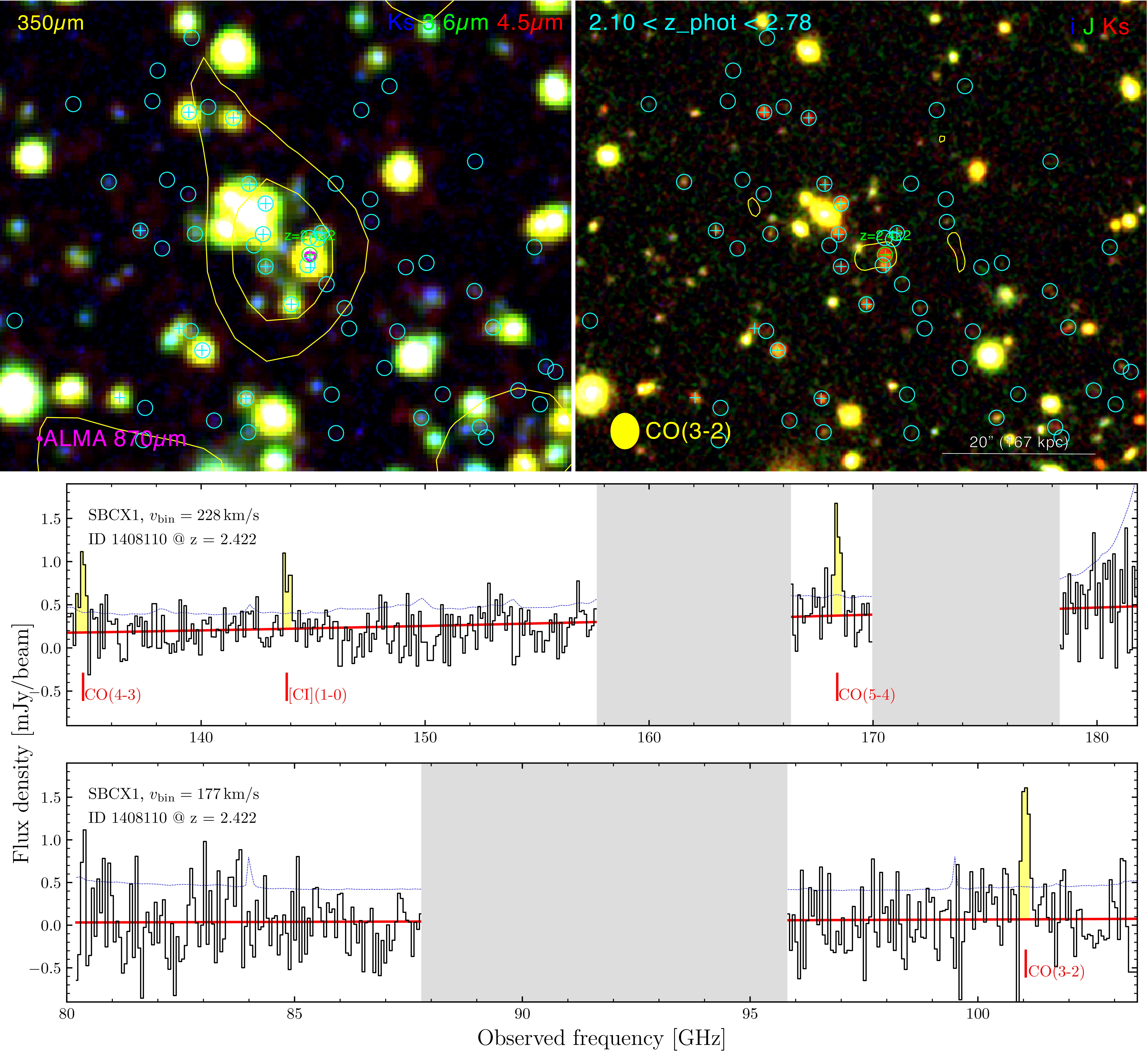
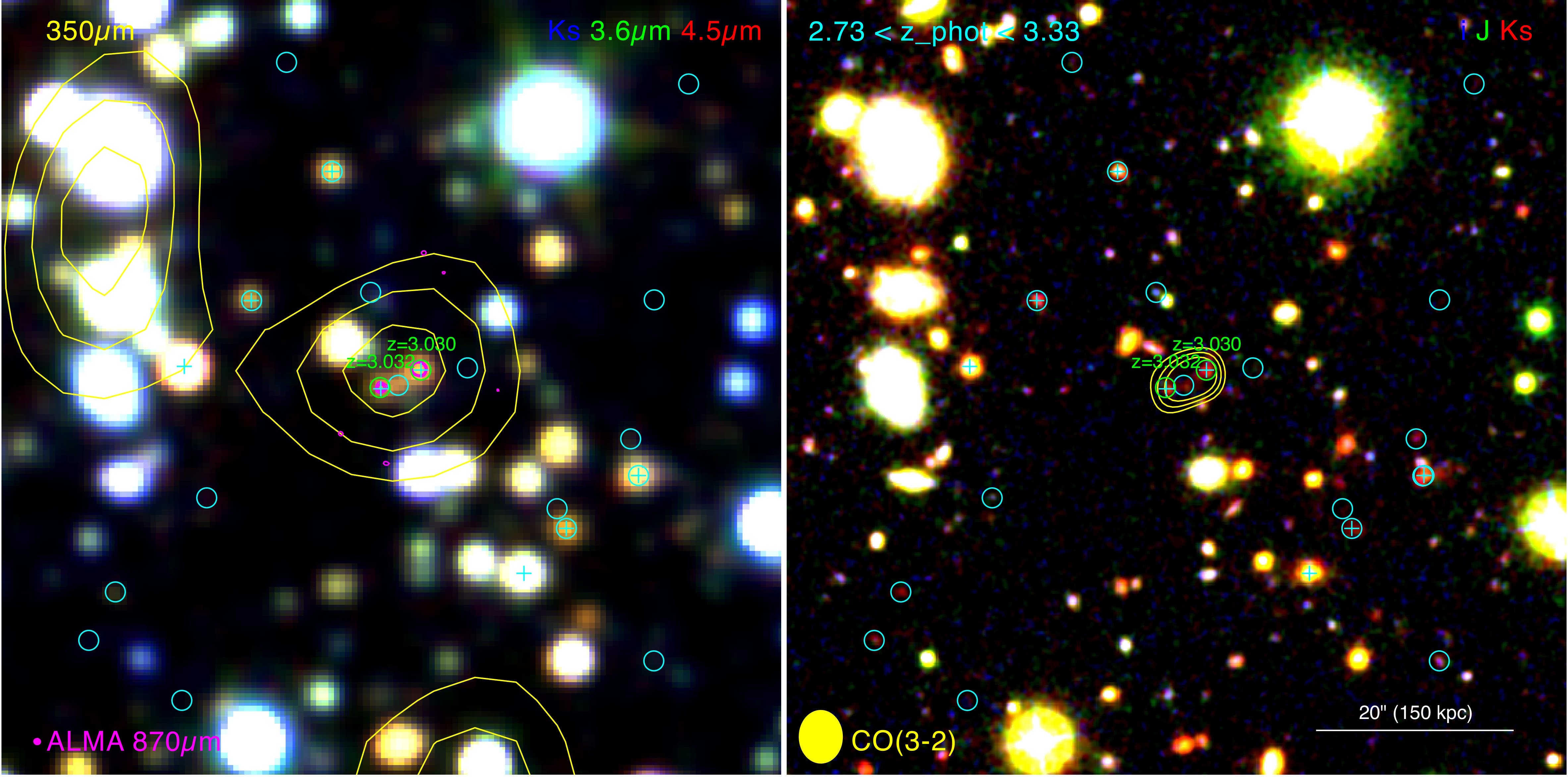
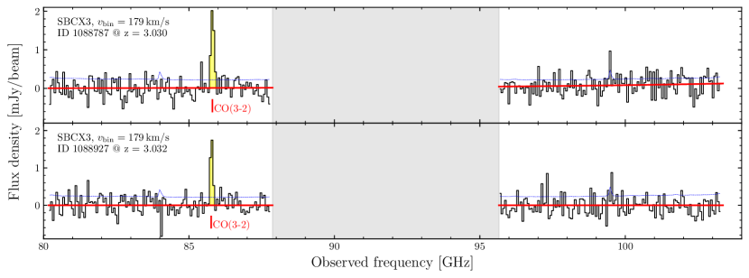

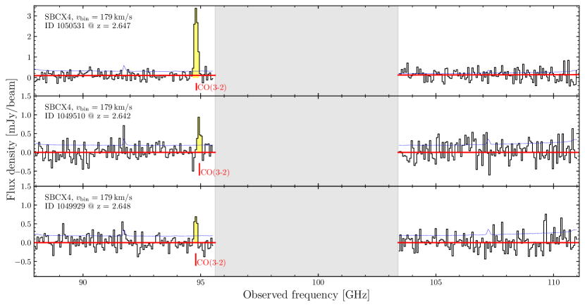

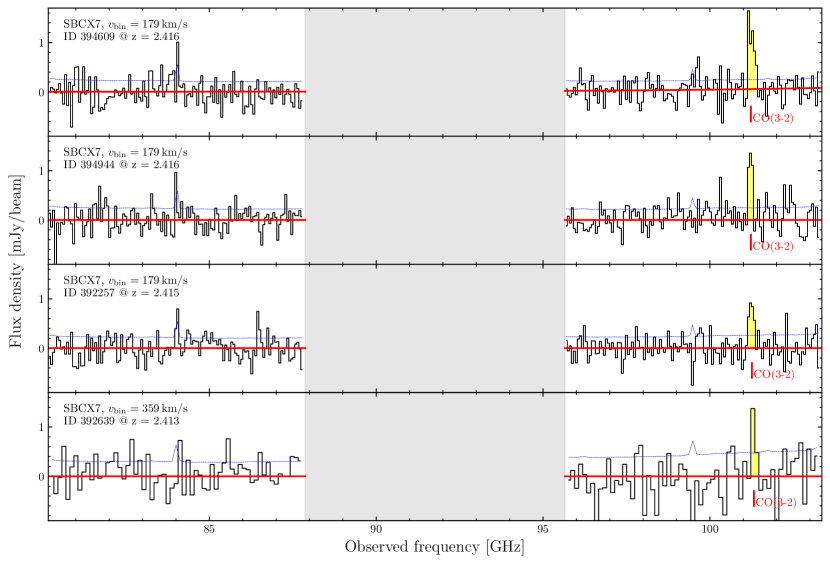
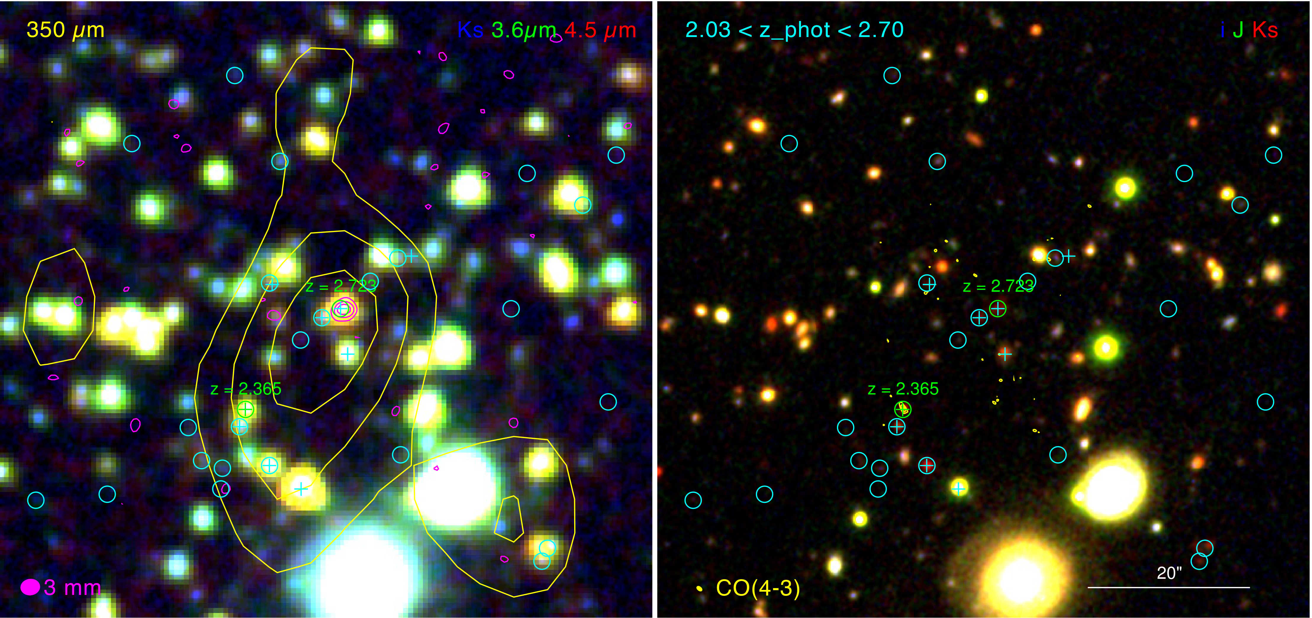

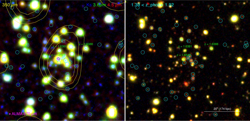
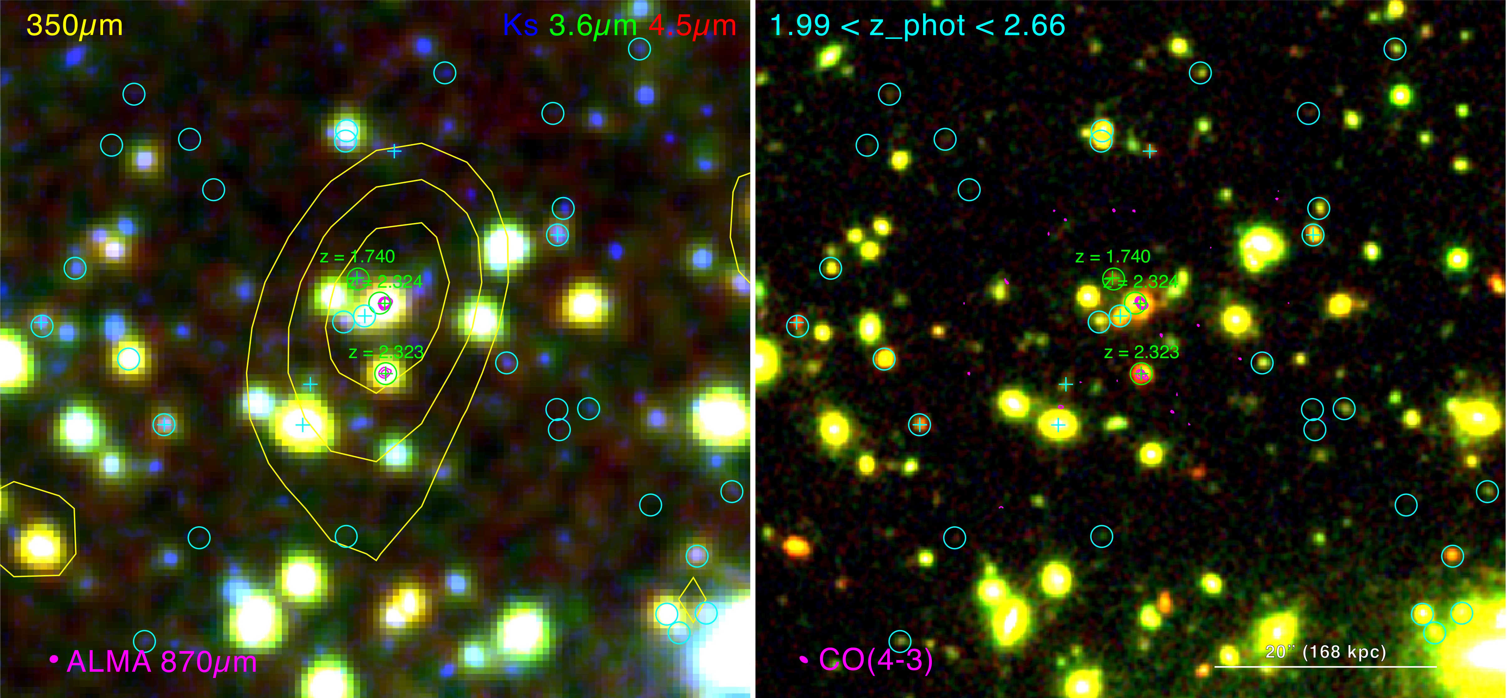
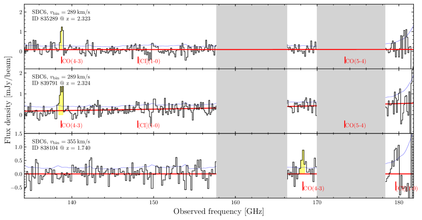
Appendix B Multi-wavelength cutouts
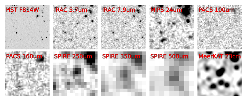
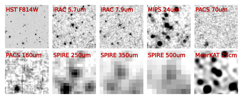
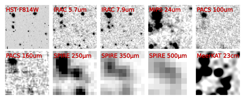
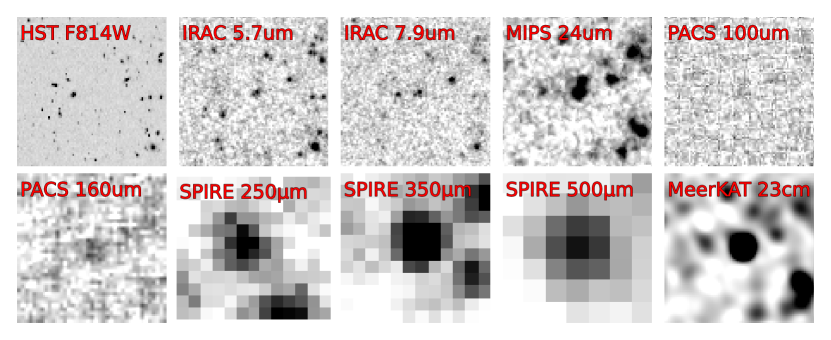
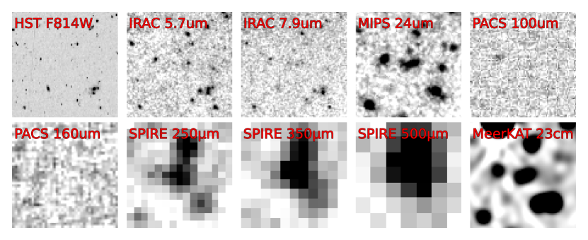
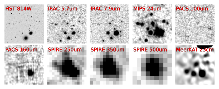
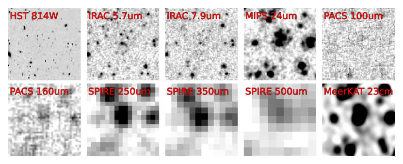
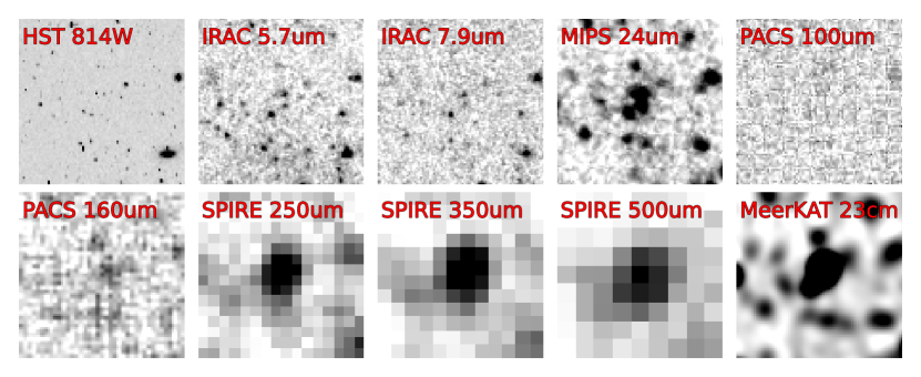
Appendix C Physical properties of individual galaxies
| Name | ID | RA | Dec. | SFR | ||||
|---|---|---|---|---|---|---|---|---|
| [deg] | [deg] | [] | [arcsec] | |||||
| (Confirmed members) | ||||||||
| HPC1001.a | – | 150.4659 | 2.6362 | – | 3.613b | |||
| HPC1001.b | 1281317 | 150.4656 | 2.6360 | 3.613b | ||||
| HPC1001.d | 1279885 | 150.4661 | 2.6361 | 3.613b | ||||
| HPC1001.la | 1274387 | 150.4647 | 2.6307 | 3.604 | ||||
| HPC1001.ma | 1272853 | 150.4618 | 2.6294 | 3.610 | ||||
| (Candidate members) | ||||||||
| HPC1001.c | 1279884 | 150.4652 | 2.6361 | – | ||||
| HPC1001.e | 1280959 | 150.4652 | 2.6366 | – | ||||
| HPC1001.f | 1280265 | 150.4654 | 2.6370 | – | ||||
| HPC1001.g | 1278992 | 150.4650 | 2.6353 | – | 3.1 | |||
| HPC1001.hc | – | 150.4655 | 2.6356 | – | ||||
| HPC1001.i | 1277620 | 150.4665 | 2.6344 | – | ||||
| HPC1001.j | 1282867 | 150.4637 | 2.6384 | – | ||||
| HPC1001.ka | 1280828 | 150.4673 | 2.6370 | – | 7.3 | |||
| 1271738 | 150.4664 | 2.6284 | – | |||||
| 1271880 | 150.4628 | 2.6283 | – | |||||
| 1273801 | 150.4611 | 2.6305 | – | |||||
| 1273919 | 150.4676 | 2.6300 | – | |||||
| 1274349 | 150.4646 | 2.6304 | – | |||||
| 1275202 | 150.4629 | 2.6318 | – | |||||
| 1278508 | 150.4686 | 2.6352 | – | |||||
| 1278832 | 150.4713 | 2.6356 | – | |||||
| 1282347 | 150.4695 | 2.6390 | – | |||||
| 1282620 | 150.4688 | 2.6393 | – | |||||
| 1286318 | 150.4700 | 2.6427 | – | |||||
| 1286772 | 150.4657 | 2.6426 | – | |||||
| 1282703 | 150.4654 | 2.6393 | – | 12.1 | ||||
| Total | – | 150.4656 | 2.6359 | – |
Notes: aNewly discovered members, not previously reported in Sillassen et al. (2022). bSources are completely blended in the NOEMA beam (Fig. 1), with a strong (S/N=10.9) and broad (Width=1824) emission line (Table 3). cSource is not in the COSMOS2020 catalogue, parameters adopted from COSMOS2015 (Laigle et al. 2016; Sillassen et al. 2022).
| ID | RA | Dec. | SFR | ||||
| [deg] | [deg] | [] | [arcsec] | ||||
| (Confirmed members) | |||||||
| 1408110 | 150.3480 | 2.7611 | 2.422 | 4.9 | |||
| (Candidate members) | |||||||
| –* | 150.3497 | 2.7619 | – | – | – | 1.9 | |
| 1398871 | 150.3534153 | 2.7532749 | – | 34.3 | |||
| 1399225 | 150.3483456 | 2.7530453 | – | 29.1 | |||
| 1399474 | 150.3479133 | 2.7530239 | – | 29.1 | |||
| 1399745 | 150.3487553 | 2.7523927 | – | 31.5 | |||
| 1399984 | 150.3541567 | 2.7542877 | – | 33.0 | |||
| 1400213 | 150.3415066 | 2.7543926 | – | 33.7 | |||
| 1400229 | 150.3470434 | 2.7545470 | – | 23.9 | |||
| 1400635 | 150.3417414 | 2.7547666 | – | 32.2 | |||
| 1401156 | 150.3540867 | 2.7554773 | – | 29.8 | |||
| 1401256 | 150.3502810 | 2.7545819 | – | 24.9 | |||
| 1401272 | 150.3395136 | 2.7556119 | – | 36.5 | |||
| 1401354 | 150.3515443 | 2.7550129 | – | 25.4 | |||
| 1401671 | 150.3472055 | 2.7559690 | – | 18.8 | |||
| 1401759 | 150.3431070 | 2.7559796 | – | 25.6 | |||
| 1401866 | 150.3403186 | 2.7561221 | – | 33.1 | |||
| 1401922 | 150.3439038 | 2.7551156 | – | 26.2 | |||
| 1402490 | 150.3503583 | 2.7558268 | – | 20.8 | |||
| 1402700 | 150.3389536 | 2.7568049 | – | 36.2 | |||
| 1402958 | 150.3452583 | 2.7569484 | – | 18.0 | |||
| 1403375 | 150.3393030 | 2.7569974 | – | 34.7 | |||
| 1404385 | 150.3465587 | 2.7584031 | – | 11.1 | |||
| 1404606 | 150.3524059 | 2.7583128 | – | 18.7 | |||
| 1404729 | 150.3519759 | 2.7575986 | – | 19.1 | |||
| 1404945 | 150.3447842 | 2.7582966 | – | 15.5 | |||
| 1405016 | 150.3467285 | 2.7591544 | – | 8.5 | |||
| 1405330 | 150.3412585 | 2.7584464 | – | 26.2 | |||
| 1405903 | 150.3473917 | 2.7600336 | – | 4.5 | |||
| 1406026 | 150.3419379 | 2.7597845 | – | 22.4 | |||
| 1406132 | 150.3487067 | 2.7592945 | – | 7.0 | |||
| 1406593 | 150.3444680 | 2.7606627 | – | 12.9 | |||
| 1406826 | 150.3496448 | 2.7606866 | – | 6.0 | |||
| 1406877 | 150.3437063 | 2.7608204 | – | 15.6 | |||
| 1407283 | 150.3481033 | 2.7607376 | – | 1.4 | |||
| 1407341 | 150.3534620 | 2.7613525 | – | 19.6 | |||
| 1407342 | 150.3397290 | 2.7614006 | – | 29.9 | |||
| 1407673 | 150.3477238 | 2.7616945 | – | 2.3 | |||
| 1407983 | 150.3500725 | 2.7614637 | – | 7.5 | |||
| 1408029 | 150.3475805 | 2.7619215 | – | 3.3 | |||
| 1408242 | 150.3542594 | 2.7620097 | – | 22.7 | |||
| 1408284 | 150.3480351 | 2.7617402 | – | 2.2 | |||
| 1408512 | 150.3457383 | 2.7623290 | – | 9.3 | |||
| 1408732 | 150.3522480 | 2.7618868 | – | 15.5 | |||
| 1409126 | 150.3457790 | 2.7631643 | – | 10.9 | |||
| 1409304 | 150.3524976 | 2.7633564 | – | 18.0 | |||
| 1409685 | 150.3470603 | 2.7637415 | – | 10.1 | |||
| 1409707 | 150.3496428 | 2.7630066 | – | 9.0 | |||
| 1409806 | 150.3532777 | 2.7638843 | – | 21.4 | |||
| 1410423 | 150.3554314 | 2.7638052 | – | 28.4 | |||
| 1410451 | 150.3502562 | 2.7637331 | – | 12.4 | |||
| 1410521 | 150.3419140 | 2.7645586 | – | 25.2 | |||
| 1412364 | 150.3508360 | 2.7661634 | – | 20.8 | |||
| 1412370 | 150.3461119 | 2.7664528 | – | 20.4 | |||
| 1412651 | 150.3538193 | 2.7667801 | – | 29.2 | |||
| 1412702 | 150.3517594 | 2.7665658 | – | 23.8 | |||
| 1412826 | 150.3524741 | 2.7663713 | – | 24.8 | |||
| 1413261 | 150.3450722 | 2.7673326 | – | 24.8 | |||
| 1413740 | 150.3536237 | 2.7679074 | – | 31.7 | |||
| 1415067 | 150.3523728 | 2.7691123 | – | 32.8 | |||
| 1415067 | 150.3523728 | 2.7691123 | – | 32.8 | |||
| Total | 150.3492 | 2.7619 | – |
Notes:*source not in the COSMOS2020 catalogue or in previous versions of COSMOS catalogues.
| ID | RA | Dec. | SFR | ||||
|---|---|---|---|---|---|---|---|
| [deg] | [deg] | [] | [arcsec] | ||||
| (Confirmed members) | |||||||
| 1088787 | 150.3105 | 2.4515 | 3.030 | 2.7 | |||
| 1088927 | 150.3117 | 2.4510 | 3.032 | 1.8 | |||
| (Candidate members) | |||||||
| 1088602 | 150.3144 | 2.4515 | – | 11.5 | |||
| 1088952 | 150.3092 | 2.4516 | – | 7.3 | |||
| 1089223 | 150.3112 | 2.4511 | – | 0.5 | |||
| 1089223 | 150.3112 | 2.4511 | – | 0.5 | |||
| 1089511 | 150.3155 | 2.4522 | – | 15.8 | |||
| 1089759 | 150.3105 | 2.4518 | – | 3.3 | |||
| 1090209 | 150.3099 | 2.4529 | – | 8.0 | |||
| 1090976 | 150.3119 | 2.4537 | – | 9.4 | |||
| Total | 150.3113 | 2.4511 | – |
| ID | RA | Dec. | SFR | ||||
|---|---|---|---|---|---|---|---|
| [deg] | [deg] | [] | [arcsec] | ||||
| Core members | |||||||
| (Confirmed members) | |||||||
| 1049510 | 150.7512 | 2.4124 | 2.642 | 2.2 | |||
| 1049929 | 150.7521 | 2.4140 | 2.648 | 5.5 | |||
| 1050531 | 150.7504 | 2.4130 | 2.647 | 1.8 | |||
| (Candidate members) | |||||||
| 1042545 | 150.7528 | 2.4067 | – | 23.4 | |||
| 1042632 | 150.7517 | 2.4069 | – | 21.7 | |||
| 1044106 | 150.7463 | 2.4083 | – | 23.3 | |||
| 1044704 | 150.7447 | 2.4088 | – | 26.6 | |||
| 1045961 | 150.7463 | 2.4097 | – | 20.0 | |||
| 1046616 | 150.7468 | 2.4107 | – | 16.6 | |||
| 1047063 | 150.7557 | 2.4108 | – | 19.3 | |||
| 1048929 | 150.7519 | 2.4124 | – | 4.5 | |||
| 1049031 | 150.7508 | 2.4131 | – | 0.8 | |||
| 1049700 | 150.7550 | 2.4138 | – | 15.4 | |||
| 1049920 | 150.7499 | 2.4134 | – | 3.8 | |||
| 1049965 | 150.7511 | 2.4141 | – | 4.3 | |||
| 1050218 | 150.7547 | 2.4143 | – | 15.0 | |||
| 1050855 | 150.7533 | 2.4143 | – | 10.4 | |||
| 1050901 | 150.7528 | 2.4150 | – | 10.2 | |||
| 1051433 | 150.7561 | 2.4155 | – | 21.3 | |||
| 1053106 | 150.7552 | 2.4169 | – | 21.5 | |||
| 1053892 | 150.7502 | 2.4173 | – | 16.1 | |||
| 1055135 | 150.7515 | 2.4190 | – | 22.2 | |||
| Total | 150.7509 | 2.4132 | – |
| ID | RA | Dec. | SFR | ||||
|---|---|---|---|---|---|---|---|
| [deg] | [deg] | [] | [arcsec] | ||||
| (Confirmed memebers) | |||||||
| 392257 | 149.9910 | 1.7967 | 2.415 | 6.0 | |||
| 392639 | 149.9816 | 1.7960 | 2.413 | 30.2 | |||
| 394609 | 149.9897 | 1.7977 | 2.416 | 0.6 | |||
| 394944 | 149.9883 | 1.7980 | 2.416 | 5.5 | |||
| (Candidate members) | |||||||
| 384203 | 149.9855 | 1.7889 | – | 33.8 | |||
| 385317 | 149.9929 | 1.7900 | – | 30.8 | |||
| 385439 | 149.9936 | 1.7900 | – | 32.1 | |||
| 385916 | 149.9957 | 1.7907 | – | 34.8 | |||
| 386678 | 149.9966 | 1.7911 | – | 35.9 | |||
| 389851 | 149.9848 | 1.7938 | – | 20.6 | |||
| 390151 | 149.9969 | 1.7944 | – | 30.7 | |||
| 390263 | 149.9957 | 1.7947 | – | 26.4 | |||
| 390843 | 149.9926 | 1.7944 | – | 17.4 | |||
| 391472 | 149.9889 | 1.7953 | – | 8.4 | |||
| 392030 | 149.9945 | 1.7965 | – | 20.1 | |||
| 392370 | 149.9939 | 1.7968 | – | 17.8 | |||
| 393623 | 149.9822 | 1.7968 | – | 24.6 | |||
| 393835 | 149.9879 | 1.7982 | – | 4.7 | |||
| 394391 | 149.9917 | 1.7981 | – | 9.8 | |||
| 396033 | 149.9907 | 1.8003 | – | 11.2 | |||
| 396633 | 149.9834 | 1.8002 | – | 22.2 | |||
| 397066 | 149.9847 | 1.8012 | – | 20.3 | |||
| 397363 | 149.9816 | 1.8016 | – | 30.2 | |||
| 397795 | 149.9903 | 1.8010 | – | 13.0 | |||
| 397953 | 149.9958 | 1.8021 | – | 29.2 | |||
| 398018 | 149.9815 | 1.8022 | – | 31.5 | |||
| 398599 | 149.9917 | 1.8027 | – | 20.7 | |||
| 398634 | 149.9882 | 1.8018 | – | 15.2 | |||
| 398787 | 149.9821 | 1.8019 | – | 29.3 | |||
| 399896 | 149.9934 | 1.8040 | – | 27.8 | |||
| 400170 | 149.9961 | 1.8043 | – | 34.8 | |||
| 400185 | 149.9890 | 1.8042 | – | 23.5 | |||
| 400413 | 149.9956 | 1.8042 | – | 33.5 | |||
| 400526 | 149.9865 | 1.8041 | – | 25.0 | |||
| 401372 | 149.9923 | 1.8054 | – | 30.3 | |||
| 401840 | 149.9904 | 1.8053 | – | 27.8 | |||
| Total | 149.9898 | 1.7978 | – |
| ID | RA | Dec. | SFR | ||||
| [deg] | [deg] | [] | [arcsec] | ||||
| (Confirmed members) | |||||||
| 1340799 | 150.7226 | 2.6963 | 2.365 | 0.0 | |||
| (Candidate members) | |||||||
| 1334731 | 150.7227768 | 2.6905261 | – | 20.9 | |||
| 1335919 | 150.7306877 | 2.6917006 | – | 33.6 | |||
| 1337358 | 150.7297781 | 2.6932095 | – | 28.2 | |||
| 1337546 | 150.7273308 | 2.6934159 | – | 20.0 | |||
| 1337712 | 150.7234355 | 2.6935964 | – | 10.3 | |||
| 1337749 | 150.7271582 | 2.6936214 | – | 19.1 | |||
| 1338883 | 150.7310329 | 2.6941766 | – | 31.4 | |||
| 1338945 | 150.7233826 | 2.6943064 | – | 7.8 | |||
| 1338973 | 150.7240954 | 2.6945682 | – | 8.3 | |||
| 1339741 | 150.7217645 | 2.6943989 | – | 7.5 | |||
| 1339910 | 150.7245508 | 2.6957013 | – | 7.4 | |||
| 1340398 | 150.7227948 | 2.6957280 | – | 2.3 | |||
| 1342336 | 150.7172687 | 2.6947672 | – | 19.9 | |||
| 1343209 | 150.7207002 | 2.6986974 | – | 10.9 | |||
| 1345593 | 150.7217632 | 2.7006506 | – | 15.9 | |||
| 1345985 | 150.7173665 | 2.7015039 | – | 26.5 | |||
| 1346174 | 150.7183122 | 2.7007088 | – | 22.1 | |||
| 1350310 | 150.7214095 | 2.7048155 | – | 30.9 | |||
| 1332724 | 150.7252518 | 2.6887611 | – | 28.9 | |||
| 1334717 | 150.7259156 | 2.6906676 | – | 23.6 | |||
| 1336266 | 150.7228321 | 2.6917998 | – | 16.3 | |||
| 1336604 | 150.7225462 | 2.6921015 | – | 15.2 | |||
| 1337924 | 150.7219464 | 2.6937675 | – | 9.5 | |||
| 1343661 | 150.7188833 | 2.6993108 | – | 17.1 | |||
| 1344343 | 150.7199699 | 2.6994621 | – | 14.7 | |||
| 1344398 | 150.7190970 | 2.6982136 | – | 14.3 | |||
| 1345139 | 150.7153071 | 2.7000313 | – | 29.4 | |||
| 1345894 | 150.7270190 | 2.7014442 | – | 24.4 | |||
| 1344398 | 150.7190970 | 2.6982136 | – | 14.3 | |||
| Total | 150.7196 | 2.6995 | – | ||||
| (Rejected members) | |||||||
| 1345246 | 150.7193 | 2.6998 | 2.723 | 15.6 |
| ID | RA | Dec. | SFR | ||||
| [deg] | [deg] | [] | [arcsec] | ||||
| (Confirmed members) | |||||||
| 840072 | 150.0368 | 2.2178 | 1.4 | ||||
| 840456 | 150.0366 | 2.2192 | 5.4 | ||||
| 840660 | 150.0325 | 2.2195 | 15.6 | ||||
| (Candidate members) | |||||||
| 824041 | 150.0366923 | 2.2061331 | – | 42.1 | |||
| 824902 | 150.0356076 | 2.2068429 | – | 39.8 | |||
| 825606 | 150.0349940 | 2.2077652 | – | 36.8 | |||
| 826524 | 150.0388680 | 2.2086292 | – | 34.0 | |||
| 826583 | 150.0294105 | 2.2087104 | – | 42.2 | |||
| 828463 | 150.0318645 | 2.2093383 | – | 35.3 | |||
| 830066 | 150.0394925 | 2.2117027 | – | 24.2 | |||
| 830220 | 150.0379440 | 2.2119681 | – | 21.6 | |||
| 830689 | 150.0275325 | 2.2092421 | – | 45.4 | |||
| 830722 | 150.0437771 | 2.2118636 | – | 33.2 | |||
| 831134 | 150.0363399 | 2.2124207 | – | 19.6 | |||
| 832008 | 150.0422681 | 2.2131902 | – | 25.9 | |||
| 832093 | 150.0353196 | 2.2132796 | – | 17.2 | |||
| 832129 | 150.0385824 | 2.2128016 | – | 19.3 | |||
| 833467 | 150.0429095 | 2.2139294 | – | 26.2 | |||
| 835280 | 150.0353156 | 2.2155435 | – | 9.8 | |||
| 835641 | 150.0353282 | 2.2149129 | – | 11.7 | |||
| 835706 | 150.0422240 | 2.2167433 | – | 20.1 | |||
| 835713 | 150.0446451 | 2.2168417 | – | 28.6 | |||
| 836069 | 150.0440213 | 2.2165815 | – | 26.5 | |||
| 836257 | 150.0366450 | 2.2172921 | – | 2.0 | |||
| 836352 | 150.0349150 | 2.2173707 | – | 6.8 | |||
| 836436 | 150.0339463 | 2.2167755 | – | 10.8 | |||
| 838011 | 150.0360963 | 2.2180155 | – | 2.5 | |||
| 838016 | 150.0430325 | 2.2189057 | – | 22.9 | |||
| 838184 | 150.0356083 | 2.2176223 | – | 4.2 | |||
| 838627 | 150.0353935 | 2.2170824 | – | 5.6 | |||
| 839179 | 150.0272763 | 2.2198195 | – | 34.9 | |||
| 839200 | 150.0346342 | 2.2186812 | – | 8.2 | |||
| 839308 | 150.0270367 | 2.2200170 | – | 35.9 | |||
| 839401 | 150.0304066 | 2.2200884 | – | 24.3 | |||
| 839911 | 150.0271665 | 2.2203543 | – | 35.7 | |||
| 840013 | 150.0450701 | 2.2178394 | – | 29.9 | |||
| 840139 | 150.0415085 | 2.2200229 | – | 18.8 | |||
| 840279 | 150.0256274 | 2.2186476 | – | 40.2 | |||
| 840962 | 150.0427285 | 2.2214865 | – | 25.2 | |||
| 841535 | 150.0411735 | 2.2214431 | – | 20.5 | |||
| 842081 | 150.0476079 | 2.2214240 | – | 41.1 | |||
| 842543 | 150.0370921 | 2.2209232 | – | 11.2 | |||
| 842559 | 150.0348747 | 2.2228335 | – | 19.2 | |||
| 842815 | 150.0378334 | 2.2231170 | – | 19.4 | |||
| 843056 | 150.0255753 | 2.2232906 | – | 44.8 | |||
| 843344 | 150.0403893 | 2.2224669 | – | 21.2 | |||
| 843499 | 150.0310788 | 2.2237657 | – | 29.6 | |||
| 843513 | 150.0358949 | 2.2221884 | – | 16.0 | |||
| 844408 | 150.0277642 | 2.2243840 | – | 40.1 | |||
| 844708 | 150.0363746 | 2.2241820 | – | 22.9 | |||
| 845635 | 150.0324820 | 2.2255824 | – | 31.9 | |||
| 845837 | 150.0438421 | 2.2257723 | – | 38.3 | |||
| 846014 | 150.0399675 | 2.2252185 | – | 29.0 | |||
| 846252 | 150.0289206 | 2.2260815 | – | 41.0 | |||
| 846409 | 150.0416911 | 2.2226615 | – | 24.8 | |||
| 846597 | 150.0425413 | 2.2241398 | – | 30.8 | |||
| 846766 | 150.0280304 | 2.2265595 | – | 44.4 | |||
| 846938 | 150.0344524 | 2.2267056 | – | 33.0 | |||
| 847198 | 150.0297779 | 2.2265661 | – | 40.2 | |||
| 847612 | 150.0388781 | 2.2273074 | – | 34.9 | |||
| 848783 | 150.0342761 | 2.2283128 | – | 38.8 | |||
| 838193 | 150.0358189 | 2.2182831 | – | 3.7 | |||
| 839977 | 150.0359993 | 2.2206550 | – | 10.5 | |||
| Total | 150.0364 | 2.2177 | – |
Notes: aspectroscopic redshifts from FMOS-COSMOS (Kashino et al. 2019).
| ID | RA | Dec. | SFR | ||||
| [deg] | [deg] | [] | [arcsec] | ||||
| (Confirmed members) | |||||||
| 835289 | 149.7053 | 2.2153 | 2.323 | 2.9 | |||
| 839791 | 149.7054 | 2.2171 | 2.324 | 4.0 | |||
| (Candidate members) | |||||||
| 829302 | 149.7100619 | 2.2111172 | – | 24.4 | |||
| 829351 | 149.7063016 | 2.2111524 | – | 17.6 | |||
| 830266 | 149.6985180 | 2.2119558 | – | 28.5 | |||
| 832418 | 149.7008521 | 2.2138819 | – | 17.8 | |||
| 833030 | 149.7009141 | 2.2143979 | – | 16.9 | |||
| 833427 | 149.7109600 | 2.2140096 | – | 21.4 | |||
| 833554 | 149.7001036 | 2.2144192 | – | 19.6 | |||
| 835393 | 149.7022002 | 2.2155898 | – | 11.4 | |||
| 835756 | 149.7058336 | 2.2167914 | – | 3.5 | |||
| 836133 | 149.7118650 | 2.2156886 | – | 23.5 | |||
| 837254 | 149.7063679 | 2.2166370 | – | 4.4 | |||
| 837789 | 149.7140782 | 2.2165296 | – | 31.5 | |||
| 838317 | 149.7132336 | 2.2180115 | – | 29.4 | |||
| 839355 | 149.7096905 | 2.2200198 | – | 21.4 | |||
| 839473 | 149.7008990 | 2.2188627 | – | 19.1 | |||
| 839572 | 149.7007529 | 2.2195411 | – | 20.9 | |||
| 840635 | 149.7123006 | 2.2211582 | – | 31.3 | |||
| 841215 | 149.7103067 | 2.2213104 | – | 26.3 | |||
| 841575 | 149.7010166 | 2.2219712 | – | 26.7 | |||
| 841712 | 149.7063190 | 2.2212635 | – | 19.4 | |||
| 843027 | 149.7062909 | 2.2215255 | – | 20.3 | |||
| 843162 | 149.7037797 | 2.2230084 | – | 26.0 | |||
| Total | 149.7057 | 2.2160 | – | ||||
| (Rejected members) | |||||||
| 838104 | 149.7060 | 2.2177 | 1.740 | 6.2 |
Appendix D Redshift probability density functions
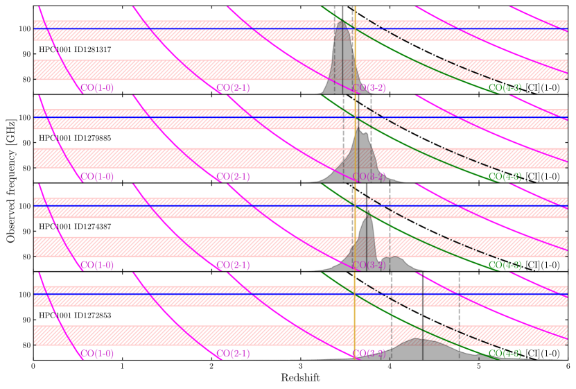
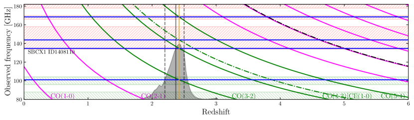
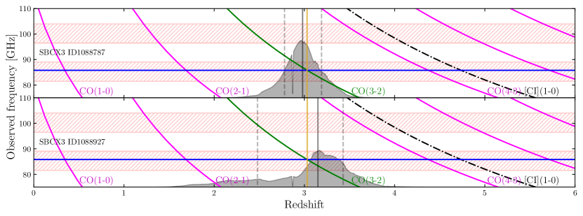
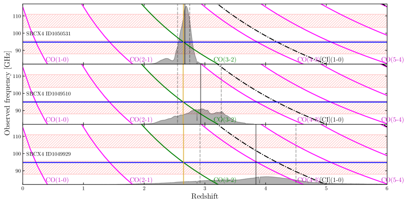
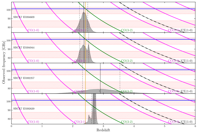
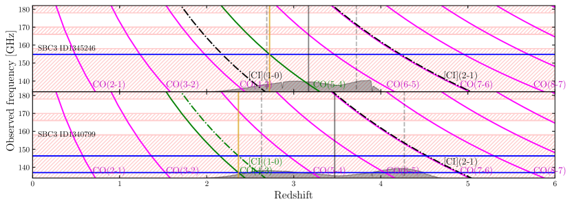
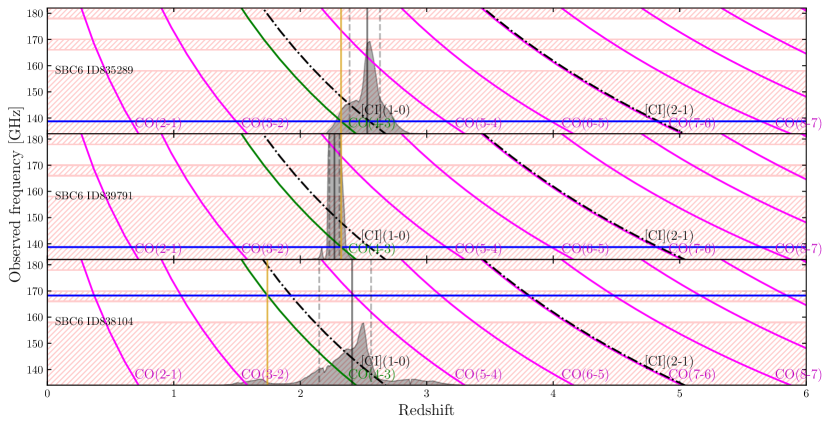
Appendix E CL-J1001 dark matter profile
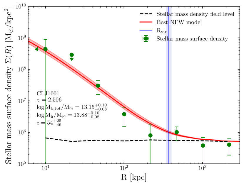
Appendix F FIR photometry
| Instrument | MIPS | PACS | PACS | SPIRE | SPIRE | SPIRE | SCUBA-2 | ALMA | ALMA/NOEMA | MeerKAT |
|---|---|---|---|---|---|---|---|---|---|---|
| Structure | ||||||||||
| HPC1001 | ||||||||||
| COS-SBCX1 | – | |||||||||
| COS-SBCX3 | ||||||||||
| COS-SBCX4 | – | |||||||||
| COS-SBCX7 | – | |||||||||
| COS-SBC3 | – | |||||||||
| COS-SBC4 | – | |||||||||
| COS-SBC6 | – |
Appendix G NFW Concentrations
| Structure | Concentration | Predictiona |
|---|---|---|
| HPC1001 | ||
| SBCX3 | ||
| SBCX4 | ||
| SBCX1 | ||
| SBCX7 | ||
| SBC3 | ||
| SBC6 | ||
| SBC4 |
Notes:apredicted concentration using concentration, halo mass, and redshift relation from Ludlow et al. (2016).
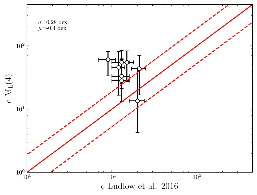
Appendix H Interloper fractions
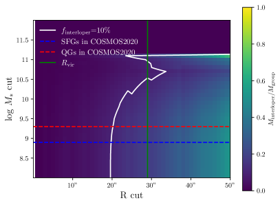
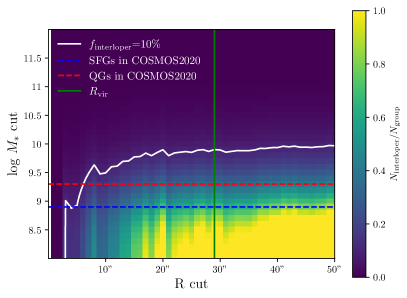
Appendix I Projected NFW profiles
Formulae for projected NFW profiles in a flat Universe, adapted from cluster_toolkit (McClintock et al. 2019)555https://github.com/tmcclintock/cluster_toolkit/.
First we define the critical density of a flat Universe at :
where is the Hubble constant, is the gravitational constant, is the matter energy fraction, is the vacuum energy fraction, and .
Then use this to define the matter density of the universe at :
Then we define the overdensity of dark matter halo:
where is the concentration parameter of the dark matter halo, and is the overdensity constant.
Next, we define the radius where the dark matter halo is times denser than the matter density of the Universe:
where is the mass contained within a sphere of with density .
Then we define the scale radius connecting and of the halo:
Next we define the shape of a line-of-sight-projected NFW profile:
Finally we combine all these parameters to define the surface density profile at radius :
And the cumulative surface density profile: