Learning Graph Structures and Uncertainty for Accurate and Calibrated Time-series Forecasting

Abstract.

Multi-variate time series forecasting is an important problem with a wide range of applications. Recent works model the relations between time-series as graphs and have shown that propagating information over the relation graph can improve time series forecasting. However, in many cases, relational information is not available or is noisy and reliable. Moreover, most works ignore the underlying uncertainty of time-series both for structure learning and deriving the forecasts resulting in the structure not capturing the uncertainty resulting in forecast distributions with poor uncertainty estimates. We tackle this challenge and introduce StoIC, that leverages stochastic correlations between time-series to learn underlying structure between time-series and to provide well-calibrated and accurate forecasts. Over a wide-range of benchmark datasets StoIC provides around 16% more accurate and 14% better-calibrated forecasts. StoIC also shows better adaptation to noise in data during inference and captures important and useful relational information in various benchmarks.

1. Introduction

While there has been a lot of work on modeling and forecasting univariate time-series (Hyndman and Athanasopoulos, 2018), the problem of multivariate time-series forecasting is more challenging. This is because modeling individual signals independently may not be sufficient to capture the underlying relationships between the signals which are essential for strong predictive performance. Therefore, many multivariate models model sparse correlations between signals based on prior knowledge of underlying structure using Convolutional networks (Li et al., 2017) or Graph Neural networks (Kipf and Welling, 2016; Zhao et al., 2019; Yu et al., 2017).

However, in many real-world applications, the graph structure is not available or is unreliable. In such cases, the problem of learning underlying patterns (Franceschi et al., 2019; Shang et al., 2021; Pamfil et al., 2020) is an active area of research (Zügner et al., 2021) in applications such as traffic prediction and energy forecasting. Most methods use a joint learning approach to train the parameters of both graph inference and forecasting modules.

However, most previous works focus only on point forecasting and do not leverage uncertainty when modeling the structure. Systematically modeling this uncertainty into the modeling pipeline can help the model adapt to unseen patterns such as when modeling a novel pandemic (Rodriguez et al., 2021). Therefore, the learned structure from existing models may not be adapted to noise in data or to distributional shifts commonly encountered in real-world datasets.

In this paper, we tackle the challenge of leveraging structure learning to provide accurate and calibrated probabilistic forecasts for all signals of a multivariate time-series. We introduce a novel probabilistic neural multivariate time-series model, StoIC (Stochastic Graph Inference for Calibrated Forecasting), that leverages functional neural process framework (Louizos et al., 2019) to model uncertainty in temporal patterns of individual time-series as well as a joint structure learning module that leverages both pair-wise similarities of time-series and their uncertainty to model the graph distribution of the underlying structure. StoIC then leverages the distribution of learned structure to provide accurate and calibrated forecast distributions for all the time-series.

Our contributions can be summarized as follows: (1) Deep probabilistic multivariate forecasting model using Joint Structure learning: We propose a Neural Process based probabilistic deep learning model that captures complex temporal and structural correlations and uncertainty over multivariate time-series. (2) State-of-art accuracy and calibration in multivariate forecasting: We evaluate StoIC against previous state-of-art models in a wide range of benchmarks and observe 16.5% more accurate and 14.7% better calibration performance. We also show that StoIC is significantly better adapted to provide consistent performance with the injection of varying degrees of noise into datasets due to modeling uncertainty. (3) Mining useful structural patterns: We provide multiple case studies to show that StoIC identifies useful domain-specific patterns based on the graphs learned such as modeling relations between stocks of the same sectors, location proximity in traffic sensors, and epidemic forecasting.

2. Methodology

Problem Formulation

Consider a multi-variate time-series dataset $\mathcal{D}$ of $N$ time-series $\mathcal{D}=\{\mathbf{y}_{i}\}_{i=1}^{N}$ over $T$ time-steps. Let $\mathbf{y}_{i}\in\mathbb{R}^{T}$ denote time-series $i$ and $y_{i}^{(t)}$ be the value at time $t$. Further, let $\mathbf{y}^{(t)}\in\mathbb{R}^{N}$ be the vector of all time-series values at time $t$. Given time-series values from till current time $t$ as $\mathbf{y}^{(1:t)}$, the goal of probabilistic multivariate forecasting is to train a model $M$ that provides a forecast distribution:

(1) $$p_{M}\left(\mathbf{y}^{(t+1:t+\tau)}|\mathbf{y}^{(1:t)};\theta\right),$$

which should be accurate, i.e, has mean close to ground truth as well as calibrated, i.e., the confidence intervals of the forecasts precisely mimic actual empirical probabilities (Fisch et al., 2022; Kamarthi et al., 2021).

Formally, the goal of joint-structure learning for probabilistic forecasting is to learn a global graph $G$ from $\mathbf{y}^{(1:t)}$ and leverage it to provide accurate and well-calibrated forecast distributions:

(2) $$p_{M}\left(\mathbf{y}^{(t+1:t+\tau)}|G,\mathbf{y}^{(1:t)};\theta\right)p_{M}\left(G|\mathbf{y}^{(1:t)};\theta\right).$$

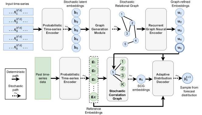
Figure 1. Overview of StoIC’s pipeline. Probabilistic Time-series encoder encodes the input time-series into stochastic latent embeddings which are used to learn the relational graph. The relational graph is leveraged by Recurrent Graph Neural Encoder to model both temporal and structural patterns of multivariate time-series represented by Graph-refined embeddings. Reference Correlation Network extracts similar patterns from past data in form of RCN embeddings. Finally, the decoder uses Graph-refined embeddings and RCN embeddings to derive the parameters of the forecast distribution.

Overview

StoIC models stochasticity and uncertainty of time-series when generating structural relations across time-series. It also adaptively leverages relations and uncertainty from past data using the functional process framework (Louizos et al., 2019; Kamarthi et al., 2021). StoIC’s generative process can be summarized as: (1) The input time-series values are encoded using a Probabilistic Time-series Encoder (PTE) that models a multivariate Gaussian Distribution to model each time-series capturing both time-series patterns and inherent uncertainty. (2) The similarity between the sampled stochastic encoding of each time-series from PTE is used to sample a graph via the Graph Generation Module (GGM). (3) Recurrent Graph Neural Encoder (RGNE) contains a series of Recurrent neural layers and Graph Convolutional Networks which derive the encoding of each time-series leveraging the learned graph. (4) We also model the similarity of encodings of input time-series with past data using a reference correlation network (RCN). (5) Finally, StoIC uses the graph-refined embeddings and historical information from RCN to learn the parameters of the output distribution.

Probabilistic Time-series Encoder

We first model both the information and uncertainty for each of the $N$ time-series, by using deep sequential models to capture complex temporal patterns of the input time-series sequence $\mathbf{y}_{i}^{(t^{\prime}:t)}$. We use a GRU (Cho et al., 2014) followed by Self-attention (Vaswani et al., 2017) over the hidden embeddings of GRU:

(3) $$\{\mathbf{\bar{h}_{i}}\}_{i=1}^{N}=\{\text{Self-Atten}(GRU(\mathbf{y}_{i}^{t^{\prime}:t}))\}_{i=1}^{N}.$$

We then model the final latent embeddings of univariate time-series as a multivariate Gaussian distribution similar to VAEs (Kingma et al., 2019):

(4) $$\mu_{\mathbf{h}_{i}},\log\sigma_{\mathbf{h}_{i}}=NN_{h}(\mathbf{\bar{h}}_{i}),\quad\mathbf{h}_{i}\sim\mathcal{N}(\mu_{\mathbf{h}_{i}},\sigma_{\mathbf{h}_{i}}).$$

where $NN_{h}$ is a single layer of feed-forward neural network. The output latent embeddings $\mathbf{H}=\{\mathbf{h}_{i}\}_{i}$ are stochastic embeddings sampled from Gaussian parameterized by $\{\mu(\mathbf{h}_{i}),\sigma(\mathbf{h}_{i})\}_{i}$. which captures uncertainty of temporal patterns.

Probabilistic Graph Generation Module

Since it is computationally expensive to model all possible relations between time-series, we aim to mine sparse stochastic relations between time-series along with the uncertainty of the underlying relations. We generate a stochastic relational graph (SRG) $G$ of $N$ nodes that model the similarity across all time-series. We use a stochastic process to generate $G$ leveraging stochastic latent embeddings $\mathbf{H}$ from PTE. We parametrize the adjacency matrix $\mathbf{A}(\mathbf{H}),\in\{0,1\}^{N\times N}$ of $G$ by modelling existence of each edge $A_{i,j}$ as a Bernoulli distribution parameterized by $\theta_{ij}$ derived as:

(5) $$\theta_{i,j}=\text{sig}(NN_{G_{2}}(NN_{G_{1}}(\mathbf{h}_{i}))+NN_{G_{1}}(\mathbf{h}_{j}))$$

where $NN_{G1}$ and $NN_{G2}$ are feed-forward networks. We sample the adjacency matrix which captures temporal uncertainty in $\mathbf{h}_{i},\mathbf{h}_{j}$ and relational uncertainty in $\theta_{i,j}$.

(6) $$(A_{i,j}=A_{j,i})\sim\text{Bernoulli}(\theta_{i,j});\forall i\leq j.$$

Recurrent Graph Neural Encoder

We combine the relational information from SRG with temporal information via a combination of Graph Neural Networks and recurrent networks:

(7) $$\mathbf{v_{i}^{(t)}}=\text{GRU-Cell}(\mathbf{u}_{i}^{(t-1)},y_{i}^{(t)});\{\mathbf{u}_{i}^{(t)}\}_{i}=GNN(\{\mathbf{v}_{i}^{(t)}\},A)$$

We input $h_{i}$ as the initial hidden embedding for GRU-Cell at initial time-step $t^{\prime}$ to impart temporal information from PTE. We finally combine the intermediate embeddings $\{\mathbf{u}_{i}^{(t)}\}_{t=t^{\prime}}^{t}$ using self-attention to get Graph-refined Embeddings $\mathbf{U}=\{\mathbf{u}_{i}\}_{i=1}^{N}$ where:

(8) $$\mathbf{u}_{i}=\text{Self-Attention}(\{\mathbf{u}_{i}^{(t)}\}_{t}).$$

Reference Correlation Network

This historical similarity is useful since time-series shows similar patterns to past data. Therefore, we model relations with past historical data of all $N$ time-series of datasets. We encode the past information of all time-series into reference embeddings $\mathbf{G}=\{\mathbf{g}_{j}\}_{j=1}^{K}$:

(9) $$\mu_{\mathbf{g}_{j}},\sigma_{\mathbf{g}_{j}}=\textsc{PTE}(\mathbf{y}_{j}^{(1:t)}),\quad\mathbf{g}_{j}\sim\mathcal{N}(\mu_{\mathbf{g}_{j}},\sigma_{\mathbf{g}_{j}}).$$

Then, similar to (Kamarthi et al., 2021) we sample edges of a bipartite Reference Correlation Network $S$ between reference embeddings $\mathbf{G}$ and Graph-refined Embeddings $\mathbf{U}$ based on their similarity as:

(10) $$\kappa(\mathbf{u}_{i},\mathbf{g}_{j})=\exp(-\gamma||\mathbf{u}_{i}-\mathbf{g}_{j}||^{2}),\quad S_{i,j}\sim\text{Bernoulli}(\kappa(\mathbf{u}_{i},\mathbf{g}_{j})).$$

where $\gamma$ is a learnable parameter. To leverage the similar reference embeddings sampled for each time-series $i$, we aggregate the sampled reference embeddings to form the RCN embeddings $\mathbf{Z}=\{\mathbf{z}_{i}\}_{i=1}^{N}$ as:

(11) $$\mathbf{z}_{i}\sim\mathcal{N}\left(\sum_{j:S_{ij}=1}NN_{z1}(\mathbf{g}_{j}),\exp(\sum_{j:S_{ij}=1}NN_{z2}(\mathbf{g}_{j}))\right)$$

where $NN_{z1}$ and $NN_{z2}$ are single fully-connected layers. Therefore, the data from reference embeddings that show similar patterns to input time-series are more likely to be sampled.

Adaptive Distribution Decoder

The decoder parameterizes the forecast distribution using multiple perspectives of information and uncertainty from previous modules: Graph-refined embeddings $\mathbf{U}$, RCN embeddings $\mathbf{Z}$ and a global embedding of all reference embeddings $g$ derived as: $\mathbf{g}=\text{Self-Attention}(\{\mathbf{g}_{j}\}_{j}).$ However, information from each of the modules may have varied importance based. Therefore, we use a weighted aggregation of these embeddings: $\mathbf{k}_{i}=l_{1}\mathbf{u}_{i}+l_{2}\mathbf{z}_{i}+l_{3}\mathbf{g}$ to get the input embedding $\mathbf{k}_{i}$ for the decoder where $\{l_{i}\}_{i=1}^{3}$ are learnable parameters. The final output forecast distribution is derived as:

(12) $$y_{i}^{(t+1)}\sim\mathcal{N}(NN_{y1}(\mathbf{k}_{i}),\exp(NN_{y2}(\mathbf{k}_{i})))$$

Training and Inference

The full generative pipeline of StoIC is:

$$\begin{split}&P(\mathbf{y^{(t+1)}}|\mathbf{y}^{t^{\prime}:t},\mathcal{D})=\int\underbrace{P(\mathbf{H}|\mathbf{y}^{t^{\prime}:t})}_{\text{Time-series Encoder}(\textsc{PTE})}\\ &\underbrace{P(A|\mathbf{H})}_{\text{Graph Generation}(\textsc{GGM})}\underbrace{P(\mathbf{U}|\mathbf{H},A)}_{\text{Recurrent Graph Neural Encoder}(\textsc{RGNE})}\\ &\underbrace{P(S,\{\mathbf{g}_{j}\}_{j}|\mathbf{U},\mathcal{D})P(\mathbf{Z}|S,\{\mathbf{g}_{j}\}_{j})}_{\text{Reference Correlation Network}(\textsc{RCN})}\underbrace{P(\mathbf{y^{(t+1)}}|\mathbf{Z,U,g})}_{\text{Decoder}}d\mathbf{H}dAd\mathbf{U}d\mathbf{g}dSd\mathbf{Z}.\end{split}$$

We train the parameters of StoIC to increase the log-likelihood loss $\log P(\mathbf{y^{(t+1)}}|\mathbf{y}^{t^{\prime}:t},\mathcal{D})$. Since integration over high-dimensional latent random variables is intractable, we use amortized variational inference like (Louizos et al., 2019) and construct the variation distribution $q(\mathbf{H,U,Z},S,A|\mathbf{y}^{t^{\prime}:t},\mathcal{D})=P(\mathbf{H}|\mathbf{y}^{t^{\prime}:t})P(A|\mathbf{H})P(S|\mathbf{U},\mathcal{D})q_{1}(\mathbf{U},\mathbf{Z}|\mathbf{y}^{t^{\prime}:t})$ where $q_{1}$ is a fully connected network over $\{\bar{\mathbf{h}}_{i}\}$ that parameterizes the variational distributions for $\mathbf{U}$ and $\mathbf{Z}$. The loss is optimized using stochastic gradient descent based Adam optimizer (Kingma and Ba, 2014). During inference, we generate Monte Carlo samples from the full distribution $P(\mathbf{y^{(t+1)}}|\mathbf{y}^{t^{\prime}:t},\mathcal{D})$ with discrete sampling.

3. Experiment Setup

Baselines

We compare with general state-of-art forecasting models that include (1) statistical models like ARIMA (Hyndman and Athanasopoulos, 2018), (2) general forecasting models: DeepAR (Salinas et al., 2020), EpiFNP (Kamarthi et al., 2021) (3) Graph-learning based forecasting models: MTGNN (Wu et al., 2020), GDN (Deng and Hooi, 2021), GTS (Shang et al., 2021), NRI (Kipf et al., 2018). Note that we are performing probabilistic forecasting while most of the baselines are modeled for point forecasts. Therefore, for methods like ARIMA, DeepAR, MTGNN and GDN, we leverage an ensemble of ten independently trained models to derive the forecast distribution (Lakshminarayanan et al., 2017).

Datasets

We evaluate our models against eight multivariate time-series datasets from a wide range of applications that have been used in past works. The main statistics of the datasets are summarized in Table 1. (1) Flu-Symptoms: We forecast a symptomatic measure of flu incidence rate based on wILI (weighted Influenza-like illness outpatients) that are provided by CDC for each of the 50 US states. We train on seasons from 2010 to 2015 and evaluate on seasons from 2015 to 2020. (2) Covid-19: We forecast the weekly incidence of Covid-19 mortality from June 2020 to March 2021 for each of the 50 US states (Rodriguez et al., 2021; Kamarthi et al., 2022) using incidence data starting from April 2020. (3) Similar to (Pamfil et al., 2020), we use the daily closing prices for stocks of companies in S& P 100 using the yfinance package (yfi, [n. d.]) from July 2014 to June 2019. The last 400 trading days are used for testing. (4) Electricity: We use a popular multivariate time-series dataset for power consumption forecasting used in past works (Zügner et al., 2021). We forecast power consumption for 15-60 minutes. We train for 1 year and test on data from the next year. (5) Traffic prediction: We use 2 datasets related to traffic speed prediction. METR-LA and PEMS-BAYS (Li et al., 2018) are datasets of traffic speed at various spots in Los Angeles and San Francisco. We use the last 10% of the time-series for testing. (6) Transit demand: NYC-Bike and NYC-Taxi (Ye et al., 2021) measure bike sharing and taxi demand respectively in New York from April to June 2016.

Table 1. Statistics of benchmark datasets

Dataset	Nodes	# time-steps	Sample rate	# Forecast horizon
Flu-Symptoms	50	544	1 week	4 weeks
Covid-19	50	44	1 week	4 weeks
S&P-100	100	1257	1 day	5 days
Electricity	321	140256	15 min.	60 min.
METR-LA	207	34272	5 min.	60 min.
PEMS-BAYS	325	52116	5 min.	60 min.
NYC-Bike	250	4368	30 min.	120 min.
NYC-Taxi	266	4368	30 min.	120 min.

Evaluation Metrics

We evaluate our model and baselines using carefully chosen metrics that are widely used in forecasting literature. They evaluate for both accuracy of the mean of forecast distributions as well as calibration of the distributions (Hyndman et al., 2006; Tsyplakov, 2013; Jordan et al., 2017). We use RMSE for point-prediction and CRPS as well as Confidence score (Kamarthi et al., 2021; Kuleshov et al., 2018; Fisch et al., 2022) for measuring forecast calibrations.

Forecast Accuracy and Calibration

Table 2. Average Evaluation Scores (over 20 runs) for StoIC and baselines. The best-performing scores are in bold and the second-best is underlined. StoIC provides around 9%, 14.7%, and 16% better performance in terms of RMSE, CS and CRPS respectively.

	Flu-Symptoms			Covid-19			S&P-100			Electricity
	RMSE	CRPS	CS	RMSE	CRPS	CS	RMSE	CRPS	CS	RMSE	CRPS	CS
ARIMA	0.85	0.91	0.22	91.5	87.4	0.21	0.42	0.40	0.27	395.2	417.2	0.37
DeepAR	0.68	0.97	0.15	49.1	48.5	0.19	0.35	0.41	0.18	249.9	267.8	0.18
EpiFNP	0.64	0.52	0.05	43.6	44.5	0.15	0.22	0.28	0.16	257.3	277.0	0.15
MTGNN	0.68	0.75	0.18	48.3	49.5	0.22	0.17	0.26	0.19	189.3	207.1	00.13
GDN	0.73	0.71	0.15	42.74	43.2	0.25	0.18	0.24	0.24	249.1	263.6	0.21
NRI	0.71	0.74	0.22	63.44	72.19	0.35	0.14	0.23	0.19	315.9	338.6	0.18
GTS	0.63	0.66	0.17	41.96	36.25	0.22	0.11	0.18	0.22	197.4	208.0	0.16
LDS	0.69	0.64	0.16	45.17	41.32	0.23	0.15	0.19	0.16	213.6	229.0	0.19
StoIC	0.57	0.42	0.07	32.7	31.7	0.2	0.11	0.16	0.12	191.6	207.3	0.09
	METR-LA			PEMS-BAYS			NYC-Bike			NYC-Taxi
	RMSE	CRPS	CS	RMSE	CRPS	CS	RMSE	CRPS	CS	RMSE	CRPS	CS
ARIMA	2.17	2.06	0.23	4.1	3.9	0.14	4.27	4.11	0.34	18.55	17.49	0.15
DeepAR	2.05	1.93	0.17	3.8	4.2	0.16	3.11	3.15	0.28	14.52	15.77	0.17
EpiFNP	2.11	1.89	0.14	4.1	3.9	0.13	2.94	2.85	0.23	15.13	14.97	0.15
MTGNN	1.86	1.64	0.14	3.2	2.9	0.11	2.62	2.61	0.17	10.37	10.13	0.13
GDN	1.95	1.83	0.16	3.4	3.1	0.16	2.74	1.78	0.15	11.15	10.64	0.17
NRI	2.17	1.95	0.19	7.9	5.3	0.14	3.18	4.7	0.36	14.38	17.52	0.31
GTS	1.88	1.74	0.15	3.7	3.2	0.13	2.76	2.85	0.24	10.75	12.68	0.18
LDS	2.12	2.05	0.13	3.5	3.7	0.18	2.55	2.67	0.21	11.44	13.98	0.19
StoIC	1.84	1.48	0.11	2.8	2.5	0.08	2.52	2.41	0.15	8.43	8.61	0.09

We evaluate the average performance of StoIC and all the baselines across 20 independent runs in Table 2. StoIC provides 8.8% more accurate forecasts (RMSE scores) across all benchmarks with an impressive 16.5% more accurate forecasts in Epidemic forecasting (Flu-Symptoms and Covid-19) and is 9% better in traffic benchmarks. For calibration, we observe significantly better CS scores across all benchmarks. StoIC also provides 16% higher CRPS scores over the best-performing baseline in each task. StoIC has 34.5% and 11.5% better performance in epidemic forecasting and traffic forecasting respectively. In particular, we also observe that baselines like ARIMA, DeepAR, and EpiFNP which do not learn a graph have 7-15% poorer performance in traffic benchmarks and over 180% poorer performance in S&P-100 benchmark compared to other baselines that learn a graph.

Robustness to Noise

We evaluate the efficacy of modeling the underlying structure of time-series and learning uncertainty of each time-series in helping models adapt to noise in the datasets. Learning a single global structure to model relations across time-series as well as modeling uncertainty in data can help the model to adapt to noise in datasets during inference. We therefore expect StoIC to be further resilient to noise in data during testing. We use the models trained on clean training time-series datasets and inject noise to time-series input during testing. Each input time-series is first independently normalized with 0 mean and unit standard deviation and then add a gaussian noise with standard deviation $\rho$.

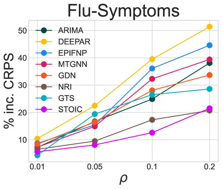
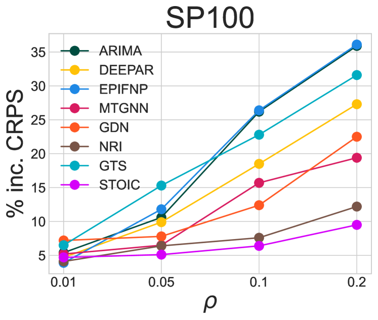
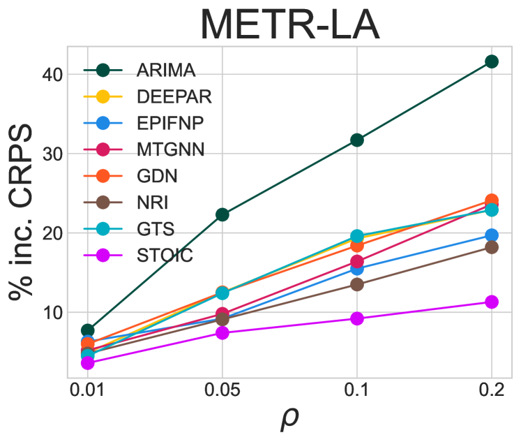
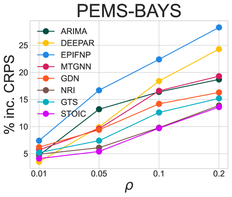
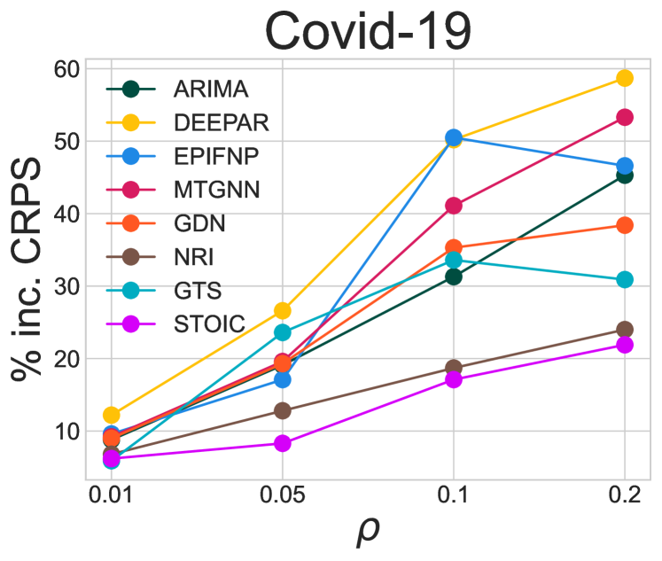
Figure 2. % increase in CRPS with an increase in gaussian Noise ($\rho$) added to the input sequence. Performance decrease of StoIC is significantly lower than most of the baselines.

We plot the decrease in performance (measured using CRPS) with an increase in noise, measured by $\rho$ in Figure 2. First, we observe that as we increase $\rho$ the performance decreases for all models. We observe that the baselines that do not learn a graph structure on average show 45-60% larger decrease in performance compared to the rest of the baselines showing the efficacy of structure learning for robust forecasting. However, StoIC’s decrease in performance is significantly less compared to most of the baselines. At $\rho=0.2$ the average performance decrease in all baselines is at 19% - 27% whereas StoIC’s performance decrease is at 9-20%. Therefore, StoIC’s ability to model uncertainty of time-series as well as effectively capture structural patterns enables it to provide forecasts that are robust to noise.

Ablation Studies

We evaluate the efficacy of various modeling choices of StoIC. Specifically, we access the influence of graph generation, RCN, and weighted aggregation (Equation 2) via ablation studies. StoIC on average outperforms all the ablation variants with 8.5% better accuracy and 3.2% better CS. Graph generation is the most impactful for performance followed by RCN. For additional details see Appendix C.

Relations Captured by Inferred Graphs

We consider various meaningful domain-specific relations for the time-series of these datasets and study how well StoIC’s inferred graphs capture them. We observed that StoIC inferred strong relations between time-series of stocks of the same sectors in S&P-100. In the case of PEMS-BAYS and METR-LA, the graph inferred by StoIC between traffic sensors is most highly correlated to actual proximity of sensors with each other compared to other baselines. Finally, the graphs inferred in Flu-Symptoms and Covid-19 are correlated with geographical adjacency of regions and road density of connecting regions. We provide more details in Appendix Section  C.1

4. Conclusion

We introduced StoIC, a probabilistic multivariate forecasting model that performs joint structure learning and forecasting leveraging uncertainty in time-series data to provide accurate and well-calibrated forecasts. We observed that StoIC performs 8.5% better in accuracy and 14.7% better in calibration over multivariate time-series benchmarks from various domains. Due to structure learning and uncertainty modeling, we also observed that StoIC better adapts to the injection of varying degrees of noise to data during inference with StoIC’s performance drop being almost half of the other state-of-art baselines. Finally, we observed that StoIC identifies useful patterns across time-series based on inferred graphs such as the correlation of stock from similar sectors, location proximity of traffic sensors and geographical adjacency and mobility patterns across US states for epidemic forecasting. While our work focuses on time-series with real values modeled as Gaussian distribution, our method can be extended to other distributions modeling different kinds of continuous signals. Further, StoIC only models a single global structure across time-series similar to most previous works. Therefore, extending our work to learn dynamic graphs that can adapt to changing underlying time-series relations or model multiple temporal scales could be an important direction for future research.

Supplementary for the paper "Learning Latent Graph Structures for Accurate and Calibrated Time-series Forecasting"

We run our models on an Nvidia Tesla V100 GPU and found that it takes less than 4 GB of memory for all benchmarks. The code for our model is available at an anonymized repository https://anonymous.4open.science/r/Stoic_KDD24-D5A8 and will be released publicly when accepted.

Appendix A Related Work

Multivariate forecasting using domain-based structural data

Deep neural networks have achieved great success in probabilistic time series forecasting. DeepAR (Salinas et al., 2020) trains an auto-regressive recurrent network to predict the parameters of the forecast distributions. Other works including deep Markov models (Krishnan et al., 2017) and deep state space models (Rangapuram et al., 2018; Li et al., 2021) explicitly model the transition and emission components with neural networks. Recently, EpiFNP (Kamarthi et al., 2021) leverages functional neural processes and achieves state-of-art performance in epidemic forecasting. However, all these methods treat each time series individually and suffer from limited forecasting performance. Leveraging the relation structure among time-series to improve forecasting performance is an emerging area. GCRN (Seo et al., 2018), DCRNN (Li et al., 2018), STGCN (Yu et al., 2017) and T-GCN (Zhao et al., 2019) adopt graph neural networks to capture the relationships among time series and provide better representations for each individual sequence. However, these methods all assume that the ground-truth graph structure is available in advance, which is often unknown in many real world applications.

Structure learning for time-series forecasting

When the underlying structure is unknown, we need to jointly perform graph structure learning and time-series forecasting. MTGNN (Wu et al., 2020) and GDN (Deng and Hooi, 2021) parameterize the graph as a degree-k graph to promote sparsity but their training can be difficult since the top-K operation is not differentiable. GTS (Shang et al., 2021) uses the Gumbel-softmax trick (Jang et al., 2016) for differentiable structure learning and uses prior knowledge to regularize the graph structure. The graph learned by GTS is a global graph shared by all the time series. Therefore, it is not flexible since it cannot adjust the graph structure for changing inputs at inference time. NRI (Kipf et al., 2018) employs a variational auto-encoder architecture and can produce different structures for different encoding inputs. It is more flexible than GTS but needs more memory to store the individual graphs. However, as previously discussed, these works do not model the uncertainty of time-series during structure learning and forecasting and do not focus on the calibration of their forecast distribution.

Appendix B Training details

The architecture of PTE and RCN is similar to (Kamarthi et al., 2021) with GRU being bi-directional and having 60 hidden units. $NN_{h},NN_{G1},NN_{G2},NN_{z1}$ and $NN_{z2}$ and GRU of RGNE also have 60 hidden units. Therefore, Graph-refined embeddings $\mathbf{U}$, RCN embeddings $\mathbf{Z}$ and global embedding $\mathbf{g}$ are 60 dimensional vectors.

We used Adam optimizer (Kingma and Ba, 2014) with a learning rate of 0.001. We found that using a batch size of 64 or 128 provided good performance with stable training. We used early stopping with patience of 200 epochs to prevent overfitting. For each of the 20 independent runs, we initialized the random seeds of all packages to 1-20. In general, variance in performance across different random seeds was not significant for all models.

Appendix C Ablation Studies

We evaluate the efficacy of various modeling choices of StoIC. Specifically, we access the influence of graph generation, RCN, and weighted aggregation (Equation 2) via the following ablation variants of StoIC:

• StoIC-NoGraph: We remove the GGM and GCN modules of RGNE and therefore do not use Graph-refined embeddings $\mathbf{U}$ in the decoder.

• StoIC-NoRefCorr: We remove the RCN module and do not use RCN embeddings $\mathbf{Z}$ in the decoder.

• StoIC-NoWtAgg: We replace weighted aggregation with concatenation in Equation 2 as

  (13) $$\mathbf{k}_{i}=\mathbf{u}_{i}\oplus\mathbf{z}_{i}\oplus\mathbf{g}$$

  where $\oplus$ is the concatenation operator.

Table 3. Average Evaluation Scores (over 20 runs) for StoIC and ablation variants.

	Flu-Symptoms			Covid-19			S&P-100			Electricity
	RMSE	CRPS	CS	RMSE	CRPS	CS	RMSE	CRPS	CS	RMSE	CRPS	CS
StoIC	0.57	0.42	0.07	32.7	31.7	0.2	0.11	0.16	0.12	191.6	207.3	0.09
StoIC-NoGraph	0.67	0.51	0.06	42.7	41.6	0.11	0.24	0.31	0.16	226.5	248.5	0.13
StoIC-NoRefCorr	0.65	0.68	0.15	44.72	40.66	0.19	0.12	0.21	0.15	196.4	211.0	0.11
StoIC-NoWtAgg	0.63	0.44	0.06	31.6	28.3	0.19	0.13	0.19	0.18	217.5	237.6	0.18
	METR-LA			PEMS-BAYS			NYC-Bike			NYC-Taxi
	RMSE	CRPS	CS	RMSE	CRPS	CS	RMSE	CRPS	CS	RMSE	CRPS	CS
StoIC	1.84	1.48	0.11	2.8	2.5	0.08	2.52	2.41	0.15	8.43	8.61	0.09
StoIC-NoGraph	2.19	1.85	0.17	3.9	4	0.15	3.41	3.16	0.19	13.65	12.89	0.21
StoIC-NoRefCorr	2.25	2.18	0.15	3.4	3.1	0.12	2.86	2.72	0.17	10.53	9.24	0.14
StoIC-NoWtAgg	1.86	1.54	0.14	3.7	3.6	0.09	2.95	2.69	0.21	9.25	8.37	0.11

Forecasting performance

As shown in Table 3, StoIC on average outperforms all the ablation variants with 8.5% better accuracy and 3.2% better CS. On average, the worst performing variant is StoIC-NoGraph followed by StoIC-NoRefCorr and StoIC-NoWtAgg, showing the importance of graph generation and leveraging learned relations across time-series.

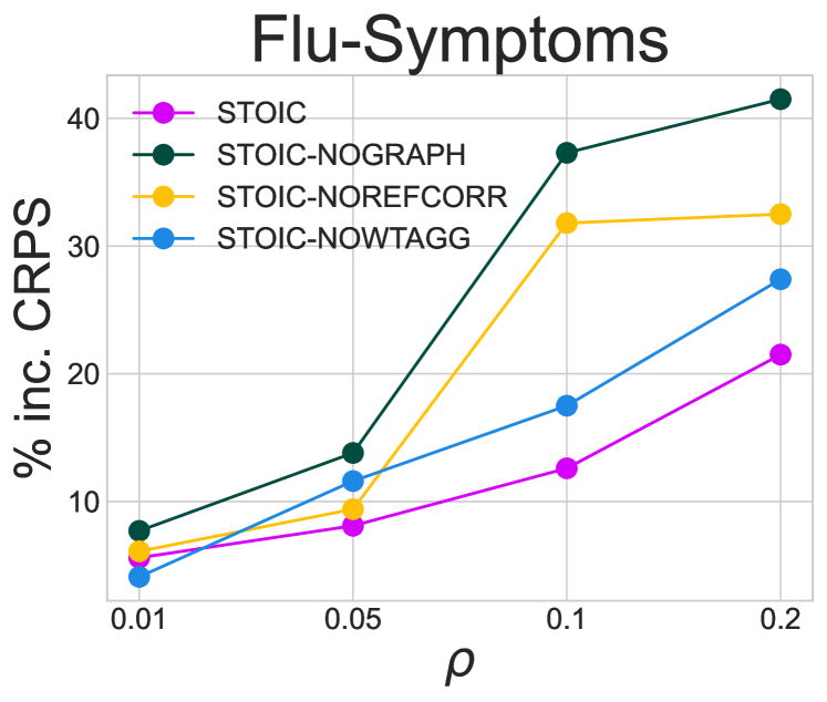
(a) Flu-Symptoms

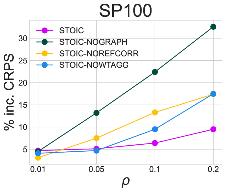
(b) S&P-100

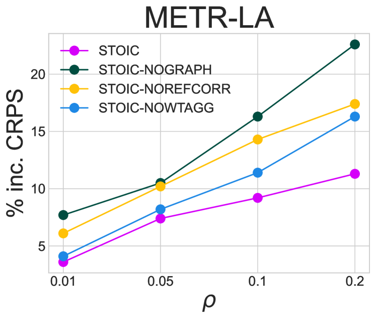
(c) METR-LA

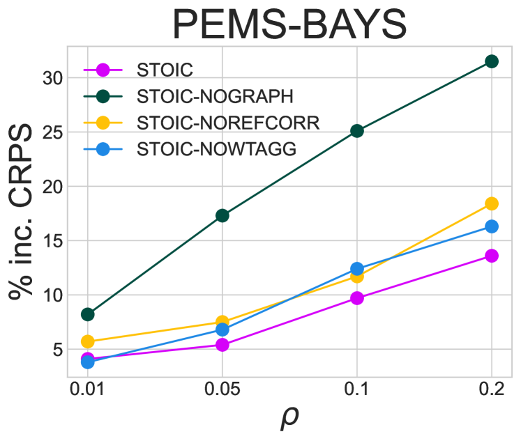
(d) PEMS-BAYS

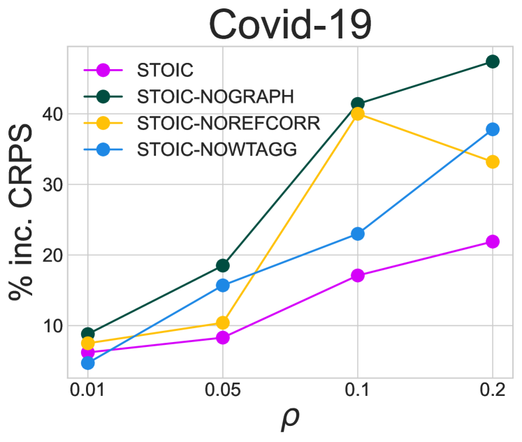
(e) Covid-19

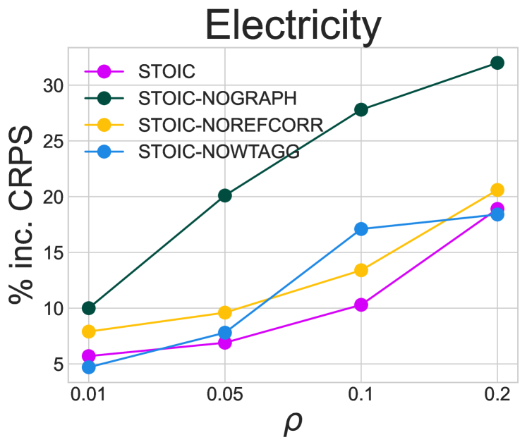
(f) Electricity

Figure 3. StoIC is better adapted to noise than other ablation variants. % increase in CRPS of StoIC and ablation variants with an increase in gaussian Noise ($\rho$) added to the input sequence.

Robustness to noise

Similar to Section 3, we also test the ablation variants’ robustness in the NFI task with performance decrease compared in Figure 3. Performance continuously decreases with an increase in $\rho$. StoIC-NoGraph is most susceptible to a decrease in performance with a 22-41% decrease in performance at $\rho=0.2$ which again shows the importance of structure to robustness. StoIC-NoRefCorr and StoIC-NoWtAgg’s performance degradation range from 15-32%. Finally, we observe that StoIC is again significantly more resilient to noise compared to all other variants.

C.1. Relations Captured by Inferred Graphs

As mentioned before, for all benchmarks there is no ‘ground-truth’ structure to compare against. However, in line with previous works (Shang et al., 2021; Pamfil et al., 2020; Wu et al., 2020; Rosensteel et al., 2021), we consider various meaningful domain-specific relations for the time-series of these datasets and study how well StoIC’s inferred graphs capture them through following case studies. Note that, for StoIC and baselines that use a sampling strategy to construct the graph (GTS, NRI, GTS, LDS), we calculate edge probability of each pair of nodes based on sampled graphs. For other graph generating baselines, we directly use the graphs inferred.

Case Study 1: Sector-level correlations of stocks in S&P-100

Two stocks representing companies from the same sectors typically influence each other more than stocks from different sectors. Therefore, we measure the correlation of edge probabilities for stocks in the same sectors. We first construct a Sector-partion graph as follows. We partition the stock time-series into sectors and construct a set of fully connected components where each component contains nodes of a sector. There are no edges across different sectors. We then measure the correlation of the edge probability matrix with the adjacency matrix of Sector-partion graph.

We observed a strong correlation score of 0.73 for graphs generated by StoIC. This was followed by graphs from GTS and LDS with correlation scores of 0.67 and 0.55. Other baselines’ graphs provided poor correlation scores below 0.35. Interestingly, this trend also correlated with the performance in forecasting with StoIC, GTS and LDS being the top three best-performing models. We also observed that the correlation score of StoIC-NoRefCorr was similar to StoIC whereas StoIC-NoWtAgg also provided low correlation scores (0.39) though their forecasting performances are comparable.

Table 4. Average edge correlation of generated graphs from the models with Sector-partition graph (for S&P-100) and proximity graph (for METR-LA and PEMS-BAYS).

	MTGNN	GDN	NIR	GTS	LDS	StoIC
S&P-100	0.05	0.42	0.34	0.67	0.55	0.73
METR-LA	0.01	0.23	0.16	0.27	0.19	0.23
PEMS-BAYS	0	0.28	0.21	0.7	0.25	0.61

Case Study 2: Identifying location proximity in traffic forecasting benchmarks

Since sensors that are located close to together may have a larger probability of showing similar or correlated signals, we study if the generated graphs capture information about the proximity of the location of the traffic sensors. We use the road location information of time-series in METR-LA and PEMS-BAYS datasets and construct the proximity graph based on pairwise road distances similar to (Zügner et al., 2021). Note that we did not feed any location-based information to the models during training.

We again measure the similarity of generated graphs with the proximity graph. We observe that GTS and StoIC provide the strongest correlation scores for both PEMS-BAYS and METR-LA datasets with average scores of 0.7 and 0.61 for PEMS-BAYS and 0.27 and 0.23 for METR-LA. Due to the lower correlation scores for METR-LA, the proximity of sensors may not be useful in modeling relations across time-series. Comparing with ablation variants, we observed that both StoIC-NoRefCorr and StoIC-NoWtAgg showed similar correlation scores to StoIC.

Case Study 3: Inferring geographical adjacency and mobility for Epidemic Forecasting

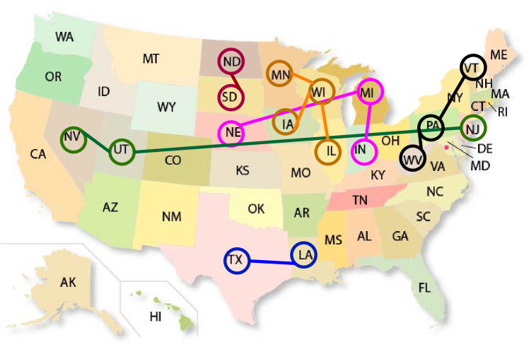
(a) Covid-19

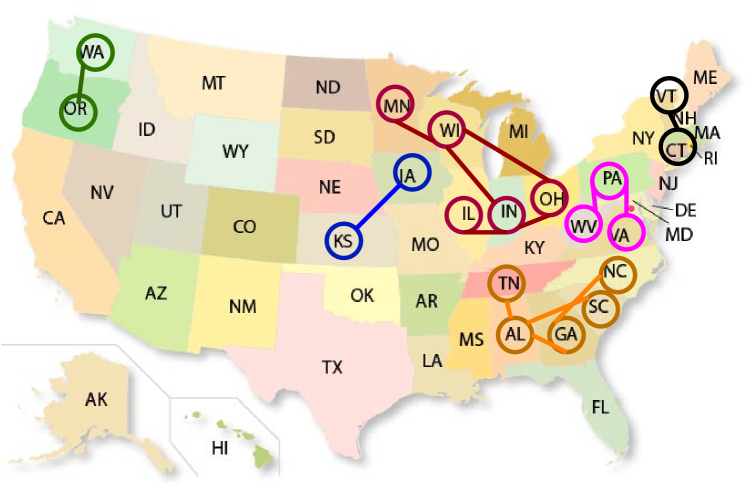
(b) Flu-Symptoms

Figure 4. Most confident edges ($\theta>0.8$) of state relation graph generated by StoIC for Epidemic Forecasting tasks. Note that most edges connect US states which have geographical proximity.

We observe the most confident edges generated by StoIC for Covid-19 and Flu-Symptoms tasks and find that most of the edges map to adjacent states or states with strong geographical proximity similar to past works (Rosensteel et al., 2021). Further, we observed that the specific states on which the graph relations are most confident are also connected by a higher density of roads with frequent commutes (Nelson and Rae, 2016). This shows that StoIC can go beyond simple patterns and infer complex mobility patterns across states leveraging past epidemic incidence data. Hence, StoIC exploits the useful relations pertaining to both geographical adjacency and mobility across these states to provide state-of-art forecasting performance.

References

- (1)
- yfi ([n. d.]) [n. d.]. yfinance · PyPI. https://pypi.org/project/yfinance/. (Accessed on 10/12/2022).
- Cho et al. (2014) Kyunghyun Cho, Bart Van Merriënboer, Dzmitry Bahdanau, and Yoshua Bengio. 2014. On the properties of neural machine translation: Encoder-decoder approaches. arXiv preprint arXiv:1409.1259 (2014).
- Deng and Hooi (2021) Ailin Deng and Bryan Hooi. 2021. Graph neural network-based anomaly detection in multivariate time series. In Proceedings of the AAAI Conference on Artificial Intelligence, Vol. 35. 4027–4035.
- Fisch et al. (2022) Adam Fisch, Tommi Jaakkola, and Regina Barzilay. 2022. Calibrated Selective Classification. arXiv preprint arXiv:2208.12084 (2022).
- Franceschi et al. (2019) Luca Franceschi, Mathias Niepert, Massimiliano Pontil, and Xiao He. 2019. Learning discrete structures for graph neural networks. In International conference on machine learning. PMLR, 1972–1982.
- Hyndman et al. (2006) Rob J Hyndman et al. 2006. Another look at forecast-accuracy metrics for intermittent demand. Foresight: The International Journal of Applied Forecasting 4, 4 (2006), 43–46.
- Hyndman and Athanasopoulos (2018) Rob J Hyndman and George Athanasopoulos. 2018. Forecasting: principles and practice. OTexts.
- Jang et al. (2016) Eric Jang, Shixiang Gu, and Ben Poole. 2016. Categorical reparameterization with gumbel-softmax. arXiv preprint arXiv:1611.01144 (2016).
- Jordan et al. (2017) Alexander Jordan, Fabian Krüger, and Sebastian Lerch. 2017. Evaluating probabilistic forecasts with scoringRules. arXiv preprint arXiv:1709.04743 (2017).
- Kamarthi et al. (2021) Harshavardhan Kamarthi, Lingkai Kong, Alexander Rodríguez, Chao Zhang, and B Aditya Prakash. 2021. When in doubt: Neural non-parametric uncertainty quantification for epidemic forecasting. Advances in Neural Information Processing Systems 34 (2021), 19796–19807.
- Kamarthi et al. (2022) Harshavardhan Kamarthi, Lingkai Kong, Alexander Rodríguez, Chao Zhang, and B Aditya Prakash. 2022. CAMul: Calibrated and Accurate Multi-view Time-Series Forecasting. In Proceedings of the ACM Web Conference 2022. 3174–3185.
- Kingma and Ba (2014) Diederik P Kingma and Jimmy Ba. 2014. Adam: A method for stochastic optimization. arXiv preprint arXiv:1412.6980 (2014).
- Kingma et al. (2019) Diederik P Kingma, Max Welling, et al. 2019. An introduction to variational autoencoders. Foundations and Trends® in Machine Learning 12, 4 (2019), 307–392.
- Kipf et al. (2018) Thomas Kipf, Ethan Fetaya, Kuan-Chieh Wang, Max Welling, and Richard Zemel. 2018. Neural relational inference for interacting systems. In International Conference on Machine Learning. PMLR, 2688–2697.
- Kipf and Welling (2016) Thomas N Kipf and Max Welling. 2016. Semi-supervised classification with graph convolutional networks. arXiv preprint arXiv:1609.02907 (2016).
- Krishnan et al. (2017) Rahul Krishnan, Uri Shalit, and David Sontag. 2017. Structured inference networks for nonlinear state space models. In Proceedings of the AAAI Conference on Artificial Intelligence, Vol. 31.
- Kuleshov et al. (2018) Volodymyr Kuleshov, Nathan Fenner, and Stefano Ermon. 2018. Accurate uncertainties for deep learning using calibrated regression. In International cuonference on machine learning. PMLR, 2796–2804.
- Lakshminarayanan et al. (2017) Balaji Lakshminarayanan, Alexander Pritzel, and Charles Blundell. 2017. Simple and scalable predictive uncertainty estimation using deep ensembles. Advances in neural information processing systems 30 (2017).
- Li et al. (2021) Longyuan Li, Junchi Yan, Xiaokang Yang, and Yaohui Jin. 2021. Learning interpretable deep state space model for probabilistic time series forecasting. arXiv preprint arXiv:2102.00397 (2021).
- Li et al. (2017) Yaguang Li, Rose Yu, Cyrus Shahabi, and Yan Liu. 2017. Diffusion convolutional recurrent neural network: Data-driven traffic forecasting. arXiv preprint arXiv:1707.01926 (2017).
- Li et al. (2018) Yaguang Li, Rose Yu, Cyrus Shahabi, and Yan Liu. 2018. Diffusion Convolutional Recurrent Neural Network: Data-Driven Traffic Forecasting. In International Conference on Learning Representations.
- Louizos et al. (2019) Christos Louizos, Xiahan Shi, Klamer Schutte, and Max Welling. 2019. The functional neural process. Advances in Neural Information Processing Systems 32 (2019).
- Nelson and Rae (2016) Garrett Dash Nelson and Alasdair Rae. 2016. An economic geography of the United States: From commutes to megaregions. PloS one 11, 11 (2016), e0166083.
- Pamfil et al. (2020) Roxana Pamfil, Nisara Sriwattanaworachai, Shaan Desai, Philip Pilgerstorfer, Konstantinos Georgatzis, Paul Beaumont, and Bryon Aragam. 2020. Dynotears: Structure learning from time-series data. In International Conference on Artificial Intelligence and Statistics. PMLR, 1595–1605.
- Rangapuram et al. (2018) Syama Sundar Rangapuram, Matthias W Seeger, Jan Gasthaus, Lorenzo Stella, Yuyang Wang, and Tim Januschowski. 2018. Deep state space models for time series forecasting. Advances in neural information processing systems 31 (2018).
- Rodriguez et al. (2021) Alexander Rodriguez, Anika Tabassum, Jiaming Cui, Jiajia Xie, Javen Ho, Pulak Agarwal, Bijaya Adhikari, and B Aditya Prakash. 2021. Deepcovid: An operational deep learning-driven framework for explainable real-time covid-19 forecasting. In Proceedings of the AAAI Conference on Artificial Intelligence, Vol. 35. 15393–15400.
- Rosensteel et al. (2021) Grant E Rosensteel, Elizabeth C Leee, Vittoria Colizza, and Shweta Bansal. 2021. Characterizing an epidemiological geography of the United States: influenza as a case study. medRxiv (2021).
- Salinas et al. (2020) David Salinas, Valentin Flunkert, Jan Gasthaus, and Tim Januschowski. 2020. DeepAR: Probabilistic forecasting with autoregressive recurrent networks. International Journal of Forecasting 36, 3 (2020), 1181–1191.
- Seo et al. (2018) Youngjoo Seo, Michaël Defferrard, Pierre Vandergheynst, and Xavier Bresson. 2018. Structured sequence modeling with graph convolutional recurrent networks. In International conference on neural information processing. Springer, 362–373.
- Shang et al. (2021) Chao Shang, Jie Chen, and Jinbo Bi. 2021. Discrete graph structure learning for forecasting multiple time series. arXiv preprint arXiv:2101.06861 (2021).
- Tsyplakov (2013) Alexander Tsyplakov. 2013. Evaluation of probabilistic forecasts: proper scoring rules and moments. Available at SSRN 2236605 (2013).
- Vaswani et al. (2017) Ashish Vaswani, Noam Shazeer, Niki Parmar, Jakob Uszkoreit, Llion Jones, Aidan N Gomez, Łukasz Kaiser, and Illia Polosukhin. 2017. Attention is all you need. Advances in neural information processing systems 30 (2017).
- Wu et al. (2020) Zonghan Wu, Shirui Pan, Guodong Long, Jing Jiang, Xiaojun Chang, and Chengqi Zhang. 2020. Connecting the dots: Multivariate time series forecasting with graph neural networks. In Proceedings of the 26th ACM SIGKDD International Conference on Knowledge Discovery & Data Mining. 753–763.
- Ye et al. (2021) Junchen Ye, Leilei Sun, Bowen Du, Yanjie Fu, and Hui Xiong. 2021. Coupled layer-wise graph convolution for transportation demand prediction. In Proceedings of the AAAI conference on artificial intelligence, Vol. 35. 4617–4625.
- Yu et al. (2017) Bing Yu, Haoteng Yin, and Zhanxing Zhu. 2017. Spatio-temporal graph convolutional networks: A deep learning framework for traffic forecasting. arXiv preprint arXiv:1709.04875 (2017).
- Zhao et al. (2019) Ling Zhao, Yujiao Song, Chao Zhang, Yu Liu, Pu Wang, Tao Lin, Min Deng, and Haifeng Li. 2019. T-gcn: A temporal graph convolutional network for traffic prediction. IEEE Transactions on Intelligent Transportation Systems 21, 9 (2019), 3848–3858.
- Zügner et al. (2021) Daniel Zügner, François-Xavier Aubet, Victor Garcia Satorras, Tim Januschowski, Stephan Günnemann, and Jan Gasthaus. 2021. A study of joint graph inference and forecasting. arXiv preprint arXiv:2109.04979 (2021).