Jacquillat and Lo

Subpath-Based Column Generation for the Electric Routing-Scheduling Problem

Subpath-Based Column Generation for the
Electric Routing-Scheduling Problem

Alexandre Jacquillat and Sean Lo Operations Research Center and Sloan School of Management, Massachusetts Institute of Technology, Cambridge, MA.

Motivated by widespread electrification targets, this paper studies an electric routing-scheduling problem (ERSP) that jointly optimizes routing-scheduling and charging decisions. The ERSP is formulated as a semi-infinite set-partitioning model, where continuous charging decisions result in infinitely-many path-based variables. To solve it, we develop a column generation algorithm with a bi-level label-setting algorithm to decompose the pricing problem into (i) a first-level procedure to generate subpaths between charging stations, and (ii) a second-level procedure to combine subpaths into paths. We formalize subpath-based domination properties to establish the finite convergence and exactness of the column generation algorithm. We prove that the methodology can handle modeling extensions with heterogeneous charging costs (via dynamic re-optimization of charging decisions) and algorithm extensions to tighten the relaxation using ng-routes and limited-memory subset-row inequalities (via augmented domination criteria). Computational results show that the methodology scales to large instances, outperforming state-of-the-art column generation algorithms. From a practical standpoint, the methodology achieves significant cost reductions by jointly optimizing routing-scheduling and charging decisions and by capturing heterogeneous charging costs.

vehicle routing, scheduling, sustainable operations, column generation, dynamic programming

1 Introduction

The climate change mitigation targets set by the International Panel on Climate Change (2023) call for widespread electrification of the economy. The share of electricity in energy use is projected to rise from 20% to nearly 30% by 2030 due to the deployment of technologies such as electric vehicles, industrial robots and heat pumps (International Energy Agency 2020). From a business perspective, electrification can mitigate the reliance on high-cost energy sources, but added acquisition costs and reduced asset utilization due to charging requirements can also hinder adoption—especially in low-margin industries. Thus, large-scale electrification requires dedicated analytics and optimization tools to efficiently and reliably deploy electrified technologies into operating systems and processes.

As part of this overarching challenge, this paper studies an electric routing-scheduling problem (ERSP) to manage a fleet of electrified machines that consume battery while performing tasks and can recharge in-between. The ERSP jointly optimizes routing-scheduling decisions (i.e., the sequence of tasks for each machine) and charging decisions (i.e., where, when, and for how long to charge). We consider a general modeling framework that can capture spatially distributed operations, heterogeneous setup and switching costs, heterogeneous charging costs, and non-linear battery consumption. This framework includes the following motivating examples:

Example 1.1 (Logistics)

Transportation and logistics are responsible for 25–30% of greenhouse gas emissions. Electric powertrains in medium- and heavy-duty trucking represent important near-term decarbonization opportunities (McKinsey & Co. 2022). The ERSP encapsulates the electric vehicle routing problem (Pelletier et al. 2016), but also augments the literature by capturing heterogeneous charging costs—an important feature in practice (Basma et al. 2023).

Example 1.2 (UAV)

Unmanned aerial vehicles (UAV) have unlocked new applications in agriculture, defense, wildfire suppression, humanitarian logistics, etc. (Drone Industry Insights 2023). The ERSP optimizes the management of an electrified UAV fleet in mission-critical environments.

Example 1.3 (Robotics)

Robotic process automation is transforming working activities, for instance in building security, manufacturing, and industrial cleaning (McKinsey Global Institute 2017). Again, the ERSP can be used to support task assignment in electrified robotic operations.

Across these applications, the ERSP combines a routing-scheduling layer and a charging layer. Routing-scheduling decisions aim to minimize operating costs subject to completion requirements; for instance, they can capture travel costs in spatially distributed routing environments, as well as setup and switching costs in machine scheduling environments. Charging decisions aim to minimize charging costs subject to battery requirements, with flexibility regarding when, where, and for how long to charge. For instance, consider a machine with a battery of 100 units, performing 10 tasks consuming 25 units each; Figures 1 shows three feasible sequences of when and by how much to recharge, for the same sequence of tasks. Altogether, the ERSP exhibits a challenging optimization structure coupling discrete routing-scheduling dynamics with continuous charging dynamics.

Figure 1: Sample routing-scheduling and charging decisions with a battery of 100 units, 10 tasks consuming 25 units. Dashed lines denote recharging actions, and solid lines denote the transitions between tasks.

We formulate the ERSP via a set-partitioning model. The model assigns each machine to a path, which encapsulates a sequence of tasks and charging decisions. In traditional routing-scheduling problems, this formulation leads to an exponential number of path-based variables, and is therefore often solved via column generation. In the ERSP, the continuous charging actions lead to an infinite number of path-based variables. The first and third examples in Figure 1 show solutions with the same routing-scheduling and charging sequence: one charges the machine with 100 units after four tasks and 50 units after six tasks; and other one charges it with 50 units after four tasks and 100 units after six tasks. In fact, infinitely-many combinations exist in-between to maintain a non-negative battery level throughout, such as the second example in Figure 1. This problem, in turn, creates a semi-infinite integer optimization structure—a challenging class of problems for which traditional column generation algorithms do not guarantee exactness and finite convergence.

The main contribution of this paper is to develop an exact, finite and scalable column generation algorithm that yields provably high-quality ERSP solutions in manageable computational times. Column generation iterates between a master problem that generates a feasible solution based on a subset of plan-based variables, and a pricing problem that identifies new variables with negative reduced cost or proves that none exists. In the ERSP, the pricing problem seeks a sequence of tasks and charging decisions, which is an NP-hard elementary resource-constrained shortest path problem (Dror 1994). It is typically modelled as a large dynamic program, and solved via label-setting algorithms with dedicated resources handling the continuous charging decisions (see Section 2). Instead, we develop a bi-level label-setting algorithm that first generates subpaths, defined as sequences of routing-scheduling decisions between charging actions, and that combines subpaths into paths by optimizing charging decisions in-between. By decomposing the pricing problem into smaller dynamic programs, we separate discrete routing-scheduling dynamics from continuous charging dynamics. As we shall establish, this approach improves the scalability of the algorithm, and provides greater flexibility in modeling heterogeneous charging costs.

Specifically, the methodology relies on three main components to decompose the pricing problem:

1. A bi-level label-setting algorithm: We propose a bi-level decomposition that first extends subpaths along edges between charging stations, and that extends sequences of subpaths into paths while optimizing charging decisions in-between. The algorithm relies on two novel elements: (i) dedicated subpath-based domination properties to prune dominated solutions throughout the algorithm; and (ii) a dynamic rebalancing procedure and dedicated domination criteria to handle heterogeneous charging costs. We prove that this algorithm returns path-based variables of negative reduced cost or guarantees that none exists.

2. A finite and exact decomposition: We prove that the column generation algorithm, armed with the bi-level label-setting algorithm for the pricing problem, yields an optimal relaxation solution in a finite number of iterations, despite the semi-infinite optimization structure of the ERSP. This result is enabled by the separation of routing-scheduling and charging decisions in the bi-level label-setting procedure.

3. Tighter relaxations: We leverage adaptive ng-relaxations to eliminate non-elementary paths that visit a customer multiple times (Baldacci et al. 2011, Martinelli et al. 2014) and limited-memory subset-row inequalities (lm-SRIs) to eliminate fractional solutions (Jepsen et al. 2008, Pecin et al. 2017). Both methods rely on “local memory” that complicate domination patterns when extending subpaths into paths. In response, we augment our bi-level label-setting algorithm with dedicated forward and backward domination criteria. We prove that the algorithm satisfies our domination properties, and therefore that the column generation methodology returns tighter ERSP relaxations with the same guarantees of exactness and finite convergence.

Through extensive computational experiments, this paper demonstrates the scalability of the optimization methodology to otherwise-intractable ERSP instances. We find that bi-level label-setting algorithm provides 50%–90% speedups against the path-based benchmark from Desaulniers et al. (2016). These improvements are most pronounced in regimes where machines need to perform many tasks but need to be recharged several times in between (i.e., each subpath spans several tasks and each path combines several subpaths). Furthermore, the augmented algorithm with adaptive ng-relaxations and lm-SRI cuts return much stronger relaxation bounds in manageable computational times. Thus, the algorithm scales to instances with up to 40 tasks and $10$ charging stations, with integrality gaps around 1-3%. From a practical standpoint, the methodology can result in significant benefits by jointly optimizing routing-scheduling and charging decisions—with up to 8% cost reduction against business-as-usual operations—and by capturing heterogeneous charging costs—with a 5–20% improvement against existing methods based on homogeneous charging costs. Ultimately, the methodology developed in this paper outperforms state-of-the-art approaches for electrified routing-scheduling optimization, and provides the first solution approach to handle heterogeneous charging costs. As such, this paper can contribute to more sustainable operations across industrial domains by easing barriers to adoption toward large-scale electrification.

2 Literature review

This paper contributes to the literature on electrified transportation and logistics. One body of work deals with the strategic problem of locating charging stations based on users’ routing choices (Arslan et al. 2019), traffic congestion (Kınay et al. 2023), car-sharing (Brandstätter et al. 2020), interactions with electricity markets (He et al. 2013), and battery swapping (Mak et al. 2013, Schneider et al. 2018, Qi et al. 2023). Kang and Recker (2015) considered the similar problem of locating refuelling stations for hydrogen vehicles. Another branch optimizes routing operations for a single vehicle, given the availability of charging stations (Sweda et al. 2017), speed-dependent operations (Nejad et al. 2017), or queuing at capacitated charging stations (Kullman et al. 2021). In-between, our paper falls into the literature on multi-vehicle electrified routing operations.

Within the vehicle routing literature, canonical problems include routing with time windows (Kallehauge et al. 2005) and capacitated vehicles (Ralphs et al. 2003). Both link discrete routing decisions and continuous timing/load decisions, but the continuous dynamics are fully determined by discrete routing decisions. In contrast, the electric vehicle routing problem (EVRP) features an extra degree of freedom to determine where, when and for how long to charge each vehicle (see Figure 1). Erdoğan and Miller-Hooks (2012) solved the EVRP using clustering-based heuristics. Schneider et al. (2014) considered the EVRP with time windows, under the restriction that all vehicles charge to full. Heuristics were developed for EVRP variants with speed-dependent battery consumption and nonlinear charging functions (Felipe et al. 2014, Goeke and Schneider 2015, Montoya et al. 2017, Fernández et al. 2022). Other models included capacitated charging stations (Froger et al. 2022), public transit (de Vos et al. 2024), and dial-a-ride (Molenbruch et al. 2023).

Exact methodologies for the EVRP rely on set-partitioning formulations along with column generation algorithms. To generate path-based variables, the pricing problem features an elementary resource-constrained shortest-path structure, and is typically solved by label-setting algorithms with dedicated domination criteria to encode charging decisions. For instance, Desaulniers et al. (2016) proposed labels for an EVRP variant with time windows; Andelmin and Bartolini (2017) used labels to model the effective range of vehicles under battery-swapping operations; and Parmentier et al. (2023) used labels modeling vehicles’ state of charge between customer visits. Our problem differs from these studies in two ways. First, motivated by long-range electrified logistics operations and other electrified applications, we do not impose time windows. This setting limits the extent of pruning in the label-setting algorithms from Desaulniers et al. (2016) and Parmentier et al. (2023). Second, we incorporate charging costs into the model, and this paper provides the first exact methodology for electric routing with heterogeneous charging costs.

These distinctions motivate our bi-level label-setting algorithm to decompose the overall (path-based) pricing problem into smaller (subpath-based) components. The main decomposition method in label-setting algorithms relies on bi-directional schemes that extend paths forward (from the source) and backward (from the sink) until they meet “in the middle” (Righini and Salani 2006). In contrast, our first-level procedure generates subpaths independently, and our second-level procedure combines them into paths. In particular, we formalize new subpath-based domination properties to guarantee exactness and finite convergence, and we propose new domination criteria to handle heterogeneous costs, ng-relaxations, and lm-SRI cuts. Interestingly, even though our label-setting algorithm is uni-directional, some of these new domination criteria require forward and backward labels to ensure the propagation of domination patterns across subpaths.

Finally, the subpath-based decomposition relates to subpath-based extended formulations in combinatorial optimization. In pickup-and-delivery or dial-a-ride, Alyasiry et al. (2019) and Zhang et al. (2023) optimized over subpaths encapsulating sequences of pickups and dropoffs from a point where the vehicle is empty to the next one; Rist and Forbes (2021) optimized over subpaths encapsulating sequences of consecutive pickups or consecutive dropoffs. Recent papers applied column generation to generate subpath-based variables dynamically (Hasan and Van Hentenryck 2021, Rist and Forbes 2022, Cummings et al. 2024). In contrast, our methodology still relies on a path-based formulation but further decomposes the pricing problem into subpaths. In other words, rather than generating subpaths on a subpath-based formulation, our approach generates subpaths on a path-based formulation. This new column generation structure requires an extra step to combine subpaths into full paths, leading to our bi-level label-setting algorithm.

3 The Electric Routing-Scheduling Problem (ERSP)

3.1 Problem Statement and Formulation

We consider a fleet of $K$ electric machines that consume battery while performing tasks, and can recharge in between. We represent operations in a directed graph $(\mathcal{V},\mathcal{A})$. Nodes are partitioned into set of depots $\mathcal{V}_{D}$, a set of tasks $\mathcal{V}_{T}$, and a set of charging stations $\mathcal{V}_{R}$, so that $\mathcal{V}=\mathcal{V}_{T}\cup\mathcal{V}_{D}\cup\mathcal{V}_{R}$. Each machine starts in a depot in $\mathcal{V}_{D}$ with full charge, performs tasks in $\mathcal{V}_{T}$, recharges in charging stations in $\mathcal{V}_{R}$, and ends in a depot. We impose a minimum number of machines $v^{\text{end}}_{j}$ ending in each depot $j\in\mathcal{V}_{D}$. Each arc $(i,j)\in\mathcal{A}$ involves a time $t(i,j)>0$, a cost $c(i,j)>0$, and a battery utilization $b(i,j)>0$, all of which satisfy the triangular inequality. The ERSP seeks a schedule for each machine to minimize operating costs, comprising traveling and charging costs, while ensuring that all tasks get performed within a planning horizon $T$. We make the following assumptions:

• All machines are homogeneous, with the same battery capacity $B$, the same travel costs, the same charging dynamics and charging costs, and the same battery depletion dynamics.

• Battery charging dynamics are linear. The charging cost per unit of time is denoted by $\delta(i)>0$ at charging station $i\in\mathcal{V}_{R}$. Through appropriate scaling, a charging time $\tau$ increases the state of charge by $\tau$ at a cost $\delta(i)\cdot\tau$. In contrast, battery depletion patterns can be non-linear.

• Charging stations are uncapacitated.

Importantly, our model can capture heterogeneous charging costs, by letting $\delta(i)$ vary across charging stations $i\in\mathcal{V}_{R}$. In the logistics example, charging costs vary based on the location of the charging station, its ownership structure, and electricity grid operations (Basma et al. 2023). As we shall see, heterogeneous charging costs impose significant complexities to the problem, so we define two variants with homogeneous and heterogeneous charging costs, referred to as ERSP-Hom and ERSP-Het respectively. We refer to ERSP for all arguments that apply to both.

The core complexity of the ERSP is to maintain appropriate charge to power all tasks. This could be achieved in integer optimization by linking binary routing variables with continuous charge variables via “big-$M$” coupling constraints. However, such formulations induce weak linear relaxations, hindering the scalability of branch-and-cut algorithms. Instead, we define a path-based ESRP formulation using Dantzig-Wolfe decomposition principles. Definition 3.1 formalizes a path as a feasible combination of routing-scheduling and charging decisions for a machine.

Definition 3.1 (Path)

A path $p$ is defined by: (i) a node sequence $U(p)=\{n_{0},n_{1},n_{2},\dots,n_{m}\}$ such that $(n_{0},n_{1}),(n_{1},n_{2}),\dots,(n_{m-1},n_{m})\in\mathcal{A}$, $n_{0}\in\mathcal{V}_{D}$, $n_{1},\dots,n_{m-1}\in\mathcal{V}_{T}\cup\mathcal{V}_{R}$, and $n_{m}\in\mathcal{V}_{D}$; and (ii) a sequence of charging times $C(p)=\Set{\tau_{k}\geq 0}{k\in\{1,\cdots,m-1\},n_{k}\in\mathcal{V}_{R}}$. The parameter $\gamma_{i}^{p}$ captures the number of times task $i\in\mathcal{V}_{T}$ is performed on path $p$: $\gamma_{i}^{p}=|\Set{k\in\Set{0,\dots,m}}{n_{k}=i}|$. For $k=0,\cdots,m$, the path $p$ reaches node $n_{k}$ at time $t_{k}$ and charge $b_{k}$, defined recursively as follows:

$$t_{0}=0\ \text{and, for all $k\in\{1,\cdots,m\}:$} t_{k} =\begin{cases}t_{k-1}+\tau_{k-1}+t(n_{k-1},n_{k})&\text{if }n_{k-1}\in\mathcal{V}_{R}\\ t_{k-1}+t(n_{k-1},n_{k})&\text{otherwise.}\end{cases}$$ (1)

$$b_{0}=B\ \text{and, for all $k\in\{1,\cdots,m\}:$} b_{k} =\begin{cases}\min\{b_{k-1}+\tau_{k-1},B\}-b(n_{k-1},n_{k})\quad&\text{if }n_{k-1}\in\mathcal{V}_{R}\\ b_{k-1}-b(n_{k-1},n_{k})&\text{otherwise.}\end{cases}$$ (2)

Path $p$ is feasible if $t_{k}\in[0,T]$ and $b_{k}\in[0,B]$ for $k=1,\cdots,m$. Its starting and ending node-time-charge triples are ($n_{\text{start}}^{p},t_{\text{start}}^{p},b_{\text{start}}^{p})=(n_{0},0,B)$ and ($n_{\text{end}}^{p},t_{\text{end}}^{p},b_{\text{end}}^{p})=(n_{m},t_{m},b_{m})$. Its cost is:

$$c^{p}=\sum_{\ell=0}^{m-1}\Big{(}c(n_{\ell},n_{\ell+1})+\mathbb{1}\left(n_{\ell}\in\mathcal{V}_{R}\right)\cdot\delta(n_{\ell})\cdot\tau_{\ell}\Big{)}$$ (3)

We define an integer decision variable $z^{p}$ tracking the number of machines assigned to path $p\in\mathcal{P}$. The ERSP minimizes costs (Equation (4)) while enforcing machines’ starting and ending locations (Equations (5) and (6)) and task requirements (Equation (7)). We refer to it as $\texttt{ERSP}(\mathcal{P})$, to its optimum as $\texttt{OPT}(\mathcal{P})$, to its linear relaxation as $\overline{\texttt{ERSP}}(\mathcal{P})$, and to its linear bound as $\overline{\texttt{OPT}}(\mathcal{P})$.

$$\min\quad \sum_{p\in\mathcal{P}}c^{p}z^{p}$$ (4)

s.t. $$\sum_{p\in\mathcal{P}}\mathbb{1}\left(n_{\text{start}}^{p}=j\right)z^{p}=v^{\text{start}}_{j} \forall\ j\in\mathcal{V}_{D}$$ (5)

$$\sum_{p\in\mathcal{P}}\mathbb{1}\left(n_{\text{end}}^{p}=j\right)z^{p}\geq v^{\text{end}}_{j} \forall\ j\in\mathcal{V}_{D}$$ (6)

$$\sum_{p\in\mathcal{P}}\gamma_{i}^{p}z^{p}=1 \forall\ i\in\mathcal{V}_{T}$$ (7)

$$z^{p}\in\mathbb{Z}_{+},\ \forall\ p\in\mathcal{P};\ \Set{p\in\mathcal{P}}{z^{p}>0}\text{ finite}$$ (8)

Note that there exist an infinite number of candidate paths due to the combination of discrete routing-scheduling decisions and continuous charging decisions. Thus, the ERSP formulation exhibits a semi-infinite integer optimization structure—a notoriously challenging class of problems. The formulation restricts the solution to a finite support for the integer variables $\{z^{p}\mid p\in\mathcal{P}\}$ to ensure that $\texttt{ERSP}(\mathcal{P})$ remains well-defined (Goberna and López-Cerdá 1998).

Per Equation (7), each task needs to be performed exactly once. Due to the triangular inequality, the formulation can be restricted to elementary paths, formalized in Definition 3.2. Proposition 3.3 shows that this restriction does not alter the integer optimization formulation but tightens its relaxation. This observation will carry great importance in our methodology.

Definition 3.2 (Elementary path)

A path $p\in\mathcal{P}$ is elementary if $\gamma_{i}^{p}\leq 1$ for all tasks $i\in\mathcal{V}_{T}$. We store all feasible paths in $\mathcal{P}_{\text{all}}$ and all elementary paths in $\mathcal{P}_{\text{elem}}\subseteq\mathcal{P}_{\text{all}}$.

Proposition 3.3

For any path set $\mathcal{P}$ with $\mathcal{P}_{\text{elem}}\subseteq\mathcal{P}\subseteq\mathcal{P}_{\text{all}}$, the following holds:

$$\overline{\texttt{OPT}}(\mathcal{P}_{\text{all}})\leq\overline{\texttt{OPT}}(\mathcal{P})\leq\overline{\texttt{OPT}}(\mathcal{P}_{\text{elem}})\leq\texttt{OPT}(\mathcal{P}_{\text{all}})=\texttt{OPT}(\mathcal{P})=\texttt{OPT}(\mathcal{P}_{\text{elem}})$$ (9)

3.2 Roadmap Toward an Exact and Finite Column Generation Algorithm

To solve the $\overline{\texttt{ERSP}}(\mathcal{P})$ relaxation, column generation iterates between a master problem that generates a feasible solution based on a subset of path-based variables (stored in $\mathcal{P}_{\ell}$ at iteration $\ell$), and a pricing problem that generates a set $\mathcal{P}_{\text{new}}$ of variables with negative reduced cost or proves that none exists (Algorithm 1). For any path $p\in\mathcal{P}$, the reduced cost of variable $z^{p}$ is

$$\overline{c}^{p}:=c^{p}-\sum_{j\in\mathcal{V}_{D}}\mathbb{1}\left(n_{\text{start}}^{p}=j\right)\kappa_{j}-\sum_{j\in\mathcal{V}_{D}}\mathbb{1}\left(n_{\text{end}}^{p}=j\right)\mu_{j}-\sum_{i\in\mathcal{V}_{T}}\gamma_{i}^{p}\nu_{i},$$ (10)

where $\bm{\kappa}$, $\bm{\mu}$, and $\bm{\nu}$ denote the dual variables associated with Equations (5), (6) and (7), respectively.

Algorithm 1 ColumnGeneration$(\mathcal{P})$.

Initialization: Construct a set of paths $\mathcal{P}_{0}\subset\mathcal{P}{}$ such that $\texttt{ERSP}(\mathcal{P}_{0})$ is feasible. Initialize $\ell=0$.

Iterate between Steps 1-3, until termination.

• Step 1. Solve $\overline{\texttt{ERSP}}(\mathcal{P}{}_{\ell})$; store optimal primal solution $\bm{z}_{\ell}$ and dual solution $(\bm{\kappa}_{\ell},\bm{\mu}_{\ell},\bm{\nu}_{\ell})$.

• Step 2. Solve pricing problem to generate paths $p\in\mathcal{P}_{\text{new}}$ with negative reduced cost (Equation (10)).

• Step 3. If $|\mathcal{P}_{\text{new}}{}|=0$, STOP: return solution $\bm{z}_{\ell}$. Otherwise, update $\mathcal{P}{}_{\ell+1}:=\mathcal{P}{}_{\ell}\cup\mathcal{P}_{\text{new}}{}$ and $\ell\leftarrow\ell+1$.

As mentioned earlier, a generic column generation scheme faces three complexities in the ERSP, which will lead to the three main contributions of our methodology:

1. Pricing problem: Column generation hinges on an efficient pricing algorithm (Step 2). We propose a bi-level label-setting algorithm that (i) generates subpaths capturing task sequences between charging decisions and (ii) combines subpaths into full paths (Sections 4.1 and 4.2).

2. Finite convergence and exactness of Algorithm 1: In traditional problems with finitely many variables, column generation is guaranteed to terminate in a finite number of iterations and to return the optimal relaxation solution. Due to the semi-infinite structure of the ERSP, however, column generation is not guaranteed to terminate finitely; moreover, upon termination, the solution is not guaranteed to be optimal if the formulation does not satisfy strong duality. We establish the finite convergence and exactness of the algorithm in Section 4.3.

3. Relaxation strength: We show that adaptive ng-routes (Baldacci et al. 2011, Martinelli et al. 2014) and lm-SRI cuts (Jepsen et al. 2008, Pecin et al. 2017) can be accommodated in our two-level label-setting algorithm via dedicated forward and backward domination criteria. Both of these extensions contribute to tightening the relaxation of the ERSP.

Upon termination, our algorithm returns an optimal solution of the $\overline{\texttt{ERSP}}(\mathcal{P})$ relaxation; we then retrieve a feasible solution to $\texttt{ERSP}(\mathcal{P})$ by restoring integrality in the master problem. In case this approach does not generate an optimal integral $\texttt{ERSP}(\mathcal{P})$ solution, the algorithm can be embedded into a branch-and-price-and-cut scheme (Barnhart et al. 1998). Notably, Desaulniers et al. (2016) branches on the number of paths, the number of charging actions, the number of stops at each charging station, and arc flows. All of these branching criteria can be handled in our framework by adding inequalities or removing arcs. Nonetheless, our computational results yield provably high-quality solutions upon termination, so we do not implement branch-and-price in this paper.

4 A Finitely-convergent Column Generation Algorithm for the ERSP

The pricing problem features an elementary resource-constrained shortest path structure. For ERSP-Hom, it can be solved via a label-setting algorithm (Desaulniers et al. 2016). This approach is described in 8 and will serve as a benchmark in this paper. However, path-based label-setting becomes intensive as paths become longer, and cannot readily handle heterogeneous charging costs in ERSP-Het. Our bi-level label-setting algorithm decomposes the pricing problem into subpaths (Section 4.1) and combines subpaths into paths (Section 4.2), as illustrated in Figure 2. We prove the exactness and finiteness of the overall column generation algorithm in Section 4.3.

(a) A path starting and ending at depots, performing tasks and recharging periodically in between.

(b) Generating subpaths.

(c) Combining subpaths into paths.

Figure 2: Bi-level label-setting: the first-level procedure extends partial subpaths along arcs; the second-level procedure extends subpath sequences along non-dominated subpaths and determines charging times.

4.1 First-level Procedure: Generating Subpaths

Definition 4.1 introduces a subpath from a non-task node (depot or charging station) to another.

Definition 4.1 (Subpath)

A subpath $s$ is defined by a node sequence $U(s)=\{n_{0},n_{1},\cdots,n_{m}\}$, such that $(n_{0},n_{1}),\cdots,(n_{m-1},n_{m})\in\mathcal{A}$, with starting node $n_{\text{start}}^{s}=n_{0}\in\mathcal{V}_{D}\cup\mathcal{V}_{R}$, intermediate nodes $n_{1},\cdots,n_{m-1}\in\mathcal{V}_{T}$, and ending node $n_{\text{end}}^{s}=n_{m}\in\mathcal{V}_{D}\cup\mathcal{V}_{R}$. The parameter $\gamma_{i}^{s}$ captures the number of times task $i\in\mathcal{V}_{T}$ is visited by the node sequence $U(s)$: $\gamma_{i}^{s}=|\Set{k\in\Set{0,\dots,m}}{n_{k}=i}|$. We define the elapsed time $t^{s}$, battery depletion $b^{s}$ and cost $c^{s}$ by: $t^{s}=\sum_{l=0}^{m-1}t(n_{l},n_{\ell+1})$, $b^{s}=\sum_{l=0}^{m-1}b(n_{l},n_{\ell+1})$, and $c^{s}=\sum_{l=0}^{m-1}c(n_{\ell},n_{\ell+1})$. Subpath $s$ is feasible if $t^{s}\in[0,T]$ and $b^{s}\in[0,B]$, and elementary if $\gamma_{i}^{s}\leq 1$ for all $i\in\mathcal{V}_{T}$. We store all feasible subpaths in $\mathcal{S}_{\text{all}}$ and all elementary subpaths in $\mathcal{S}_{\text{elem}}\subseteq\mathcal{S}_{\text{all}}$.

One difference between subpaths and paths is that a subpath can start and end at a charging stations, and must only visit task nodes in between. Another difference is that subpaths do not encapsulate charging decisions. Thus, subpath decomposition decouples routing-scheduling vs. charging decisions. The set of subpaths is therefore finite, in contrast with the infinitely-sized set of paths. Nonetheless, there exist an infinite number of possible charging decisions between subpaths, hence an infinite number of possible combinations of subpaths into full paths.

The first-level dynamic programming procedure generates non-dominated subpaths, using standard label-setting arguments to optimize routing-scheduling decisions between a starting node and an ending node. This procedure extends partial subpaths along arcs until a depot or a charging station is reached. A partial subpath (resp. partial path) is defined similarly to a subpath (resp. path) except that the condition $n_{\text{end}}^{s}\in\mathcal{V}_{D}\cup\mathcal{V}_{R}$ (resp. $n_{\text{end}}^{p}\in\mathcal{V}_{D}$) is relaxed. We denote by $\mathcal{S}^{\circ}$ and $\mathcal{P}^{\circ}$ the set of feasible partial subpaths from $\mathcal{S}$ and of feasible partial paths from $\mathcal{P}$. For example, $\mathcal{S}_{\text{all}}^{\circ}$ stores all feasible partial subpaths and $\mathcal{S}_{\text{elem}}^{\circ}$ stores all elementary feasible partial subpaths.

Definition 4.2 (Extensions of partial subpaths)

Consider a feasible partial subpath $s\in\mathcal{S}^{\circ}$ with node sequence $\{n_{0},\cdots,n_{m}\}$ such that $n_{\text{end}}^{s}=n_{m}\notin\mathcal{V}_{D}\cup\mathcal{V}_{R}$. For any arc $a=(n_{\text{end}}^{s},n_{\text{next}})\in\mathcal{A}$, we denote by $s\oplus a$ the extended partial subpath defined by the node sequence $\{n_{0},\cdots,n_{m},n_{\text{next}}\}$. The extension is feasible if $t^{s}+t(n_{m},n_{\text{next}})\leq T$ and $b^{s}+b(n_{m},n_{\text{next}})\leq B$.

Definition 4.3 (Reduced cost contribution: subpath)

Given dual variables $\bm{\kappa}$, $\bm{\mu}$, and $\bm{\nu}$, the reduced cost contribution $\widehat{c}^{s}$ of a partial subpath $s$ visiting $n_{0},\cdots,n_{m}$ is defined as:

$$\widehat{c}^{s} =\sum_{l=0}^{m-1}\left(c(n_{\ell},n_{\ell+1})-\mathbb{1}\left(n_{\ell+1}\in\mathcal{V}_{T}\right)\nu_{n_{\ell+1}}\right)\ -\mathbb{1}\left(n_{0}\in\mathcal{V}_{D}\right)\kappa_{n_{0}}-\mathbb{1}\left(n_{m}\in\mathcal{V}_{D}\right)\mu_{n_{m}}$$ (11)

Note that the reduced cost contributions, defined for partial subpaths, do not coincide with the reduced costs of decision variables, defined for paths. Rather, the reduced cost of a path is decomposable into the reduced cost contributions of its constituent subpaths plus the charging costs between subpaths (see Lemma 4.8 later on). Importantly, the reduced cost contribution is decomposable across arcs, which will enable to generate subpaths via dynamic programming.

We eliminate partial subpaths that cannot be part of a path of minimum reduced cost by applying domination criteria (Definition 4.4). Property 4.4 specifies an important property that needs to be satisfied by the domination criteria—namely, that domination patterns must propagate along arc extensions. For completeness, we also provide in Property 9 technical criteria that are necessary to ensure termination and exactness. Proposition 4.5 provides domination and non-domination criteria for the ERSP that satisfy these domination and termination properties.

Definition 4.4 (Subpath domination)

Let $(\mathrm{D^{s}}\left(\cdot\right),\mathrm{ND^{s}}\left(\cdot\right),\mathcal{S})$ define vectors of domination and non-domination criteria with respect to set $\mathcal{S}$. Partial subpath $s_{1}$ dominates $s_{2}$, written $s_{1}\succeq_{s}s_{2}$ if $\mathrm{ND^{s}}\left(s_{1}\right)=\mathrm{ND^{s}}\left(s_{2}\right)$ and $\mathrm{D^{s}}\left(s_{1}\right)\leq\mathrm{D^{s}}\left(s_{2}\right)$ component-wise. Partial subpath $s$ is non-dominated if no partial subpath $s^{\prime}\in\mathcal{S}^{\circ}$ satisfies $s^{\prime}\succeq_{s}s$. Let $\widetilde{\mathcal{S}}$ store the set of non-dominated subpaths, and $\widetilde{\mathcal{S}^{\circ}}$ store the set of non-dominated partial subpaths out of all subpaths in $\mathcal{S}$.

[Domination criteria for subpaths] $(\mathrm{D^{s}}\left(\cdot\right),\mathrm{ND^{s}}\left(\cdot\right),\mathcal{S})$ must satisfy:

1. For feasible partial subpaths $s_{1},s_{2}\in\mathcal{S}^{\circ}$ such that $s_{1}\succeq_{s}s_{2}$, and an extension $a\in\mathcal{A}$ of $s_{1}$ and $s_{2}$, either (a) $s_{2}\oplus a\notin\mathcal{S}^{\circ}$, or (b) $s_{1}\oplus a\in\mathcal{S}^{\circ}$, $s_{2}\oplus a\in\mathcal{S}^{\circ}$, and $s_{1}\oplus a\succeq_{s}s_{2}\oplus a$.

Proposition 4.5

The following criteria satisfy Properties 4.4 and 9:

For $$\mathcal{P}=\mathcal{P}_{\text{all}} \mathrm{ND^{s}}\left(s\right)=(n_{\text{start}}^{s},n_{\text{end}}^{s}), \mathrm{D^{s}}\left(s\right)=(\widehat{c}^{s},t^{s},b^{s}),$$: (12)

For $$\mathcal{P}=\mathcal{P}_{\text{elem}} \mathrm{ND^{s}}\left(s\right)=(n_{\text{start}}^{s},n_{\text{end}}^{s}), \mathrm{D^{s}}\left(s\right)=(\widehat{c}^{s},t^{s},b^{s},\{\gamma_{i}^{s}\}_{i\in\mathcal{V}_{T}}).$$: (13)

An arc extension $a=(n_{\text{end}}^{s},n_{\text{next}})$ of subpath $s$ yields the following updates:

$$\mathrm{ND^{s}}\left(s\oplus a\right) =(n_{\text{start}}^{s},n_{\text{next}})$$ (14)

$$\widehat{c}^{s\oplus a} =\widehat{c}^{s}+c(n_{\text{end}}^{s},n_{\text{next}})-\mathbb{1}\left(n_{\text{next}}\in\mathcal{V}_{T}\right)\nu_{n_{\text{next}}}-\mathbb{1}\left(n_{\text{next}}\in\mathcal{V}_{D}\right)\mu_{n_{\text{next}}}$$ (15)

$$t^{s\oplus a} =t^{s}+t(n_{\text{end}}^{s},n_{\text{next}})$$ (16)

$$b^{s\oplus a} =b^{s}+b(n_{\text{end}}^{s},n_{\text{next}})$$ (17)

$$\gamma_{i}^{s\oplus a} =\gamma_{i}^{s}+\mathbb{1}\left(n_{\text{next}}=i\right),\quad\forall\ i\in\mathcal{V}_{T}\quad\text{(for $\mathcal{P}=\mathcal{P}_{\text{elem}}$)}$$ (18)

Without elementarity, the algorithm maintains three domination criteria: reduced cost, time, and battery consumption. Thus, a subpath is dominated if another one ends in the same node earlier, using less charge, and contributing a smaller reduced cost. Elementarity requirements impose an extra label per task, which severely hinders tractability. This section proposes a two-level label-setting algorithm that can generate non-dominated paths in $\mathcal{P}_{\text{all}}$ (with three-dimensional labels) or in $\mathcal{P}_{\text{elem}}$ (with high-dimensional labels); we address elementarity requirements in Section 5.1.

Algorithm 2 presents the first-level label-setting procedure. Starting at any non-task node (depot or charging station), it extends partial subpaths along arcs while ensuring feasibility and pruning all dominated partial subpaths, until reaching a depot or a charging station. Throughout, it maintains a set $\mathcal{S}_{\text{gen}}$ of non-dominated partial subpaths and a queue $\mathcal{S}_{\text{queue}}$ of partial subpaths. It is parametrized by the domination and non-domination criteria and the set of feasible subpaths. In particular, elementarity can be imposed by setting $\mathcal{S}=\mathcal{S}_{\text{elem}}$ or relaxed by setting $\mathcal{S}=\mathcal{S}_{\text{all}}$. Note that, despite the infinite set of paths, any partial subpath has finitely many extensions, and FindNonDominatedSubpaths converges finitely (this will be proved in Section 4.3).

Algorithm 2 FindNonDominatedSubpaths$\big{(}\mathrm{D^{s}}\left(\cdot\right),\mathrm{ND^{s}}\left(\cdot\right),\mathcal{S}\big{)}$.

Initialization: $\mathcal{S}_{\text{gen}}=\emptyset$; store in $\mathcal{S}_{\text{queue}}$ all single-node partial subpaths starting at nodes $i\in\mathcal{V}_{D}\cup\mathcal{V}_{R}$.

• Step 1. Select $s\in\mathcal{S}_{\text{queue}}$ with smallest time stamp: $s\in\argmin\Set{t^{s}}{s\in\mathcal{S}_{\text{queue}}}$. Remove $s$ from $\mathcal{S}_{\text{queue}}$, and add it to $\mathcal{S}_{\text{gen}}$. If $s$ is a subpath, go to Step 3. Else, go to Step 2.

• Step 2. For each arc extension $a=(n_{\text{end}}^{s},n_{\text{next}})\in\mathcal{A}$ of $s$:

  1. If $s\oplus a\notin\mathcal{S}^{\circ}$, or if there exists $s^{\prime}\in\mathcal{S}_{\text{queue}}\cup\mathcal{S}_{\text{gen}}$ such that $s^{\prime}\succeq_{s}s\oplus a$, continue.

  2. Otherwise, remove any $s^{\prime}\in\mathcal{S}_{\text{queue}}$ such that $s\oplus a\succeq_{s}s^{\prime}$, and add $s\oplus a$ to $\mathcal{S}_{\text{queue}}$.

• Step 3. If $\mathcal{S}_{\text{queue}}=\emptyset$, STOP: return $\set{s\in\mathcal{S}_{\text{gen}}}{s\text{ is a subpath}}$. Otherwise, go to Step 1.

4.2 Second-level Procedure: Combining Subpaths into Paths

Preliminaries.

The second-level procedure optimizes routing-scheduling decisions by extending subpath sequences along subpaths, and optimizes charging decisions between subpaths. Throughout, it also applies domination criteria to eliminate dominated subpath sequences.

Definition 4.6 (Subpath sequence)

A subpath sequence $\sigma=\{s_{1},\dots,s_{m}\}$ satisfies $s_{1},\dots,s_{m}\in\mathcal{S}$, $n_{\text{start}}^{\sigma}=n_{\text{start}}^{s_{1}}\in\mathcal{V}_{D}$, $n_{\text{end}}^{s_{i}}=n_{\text{start}}^{s_{i+1}}\in\mathcal{V}_{R}$ for $i\in\{1,\cdots,m-1\}$, and $n_{\text{end}}^{\sigma}=n_{\text{end}}^{s_{m}}\in\mathcal{V}_{D}\cup\mathcal{V}_{R}$. It is feasible if there exists a feasible partial path $p\in\mathcal{P}^{\circ}$ with subpath sequence $\sigma$; and it is complete if $n_{\text{end}}^{\sigma}\in\mathcal{V}_{D}$. Let ${\bm{\mathcal{S}}^{\circ}}$ (resp. $\SS$) store feasible (resp. feasible complete) subpath sequences. Let $\mathcal{P}^{\circ}(\sigma)\subseteq\mathcal{P}^{\circ}$ (resp. $\mathcal{P}(\sigma)\subseteq\mathcal{P}$) store feasible partial paths (resp. feasible paths) with subpath sequence $\sigma$.

By construction, all partial paths sharing a subpath sequence differ only in charging times. Lemma 4.8 proves that the reduced cost of a path is decomposable into the reduced cost contribution of its subpath sequence and the charging costs between subpaths.

Definition 4.7 (Reduced cost contribution: path)

A feasible partial path $p\in\mathcal{P}^{\circ}$ with subpath sequence $\sigma=\{s_{1},\dots,s_{m}\}$ and charging times $\{\tau_{1},\dots,\tau_{m-1}\}$ has reduced cost contribution

$$\widehat{c}^{p}:=\sum_{i=1}^{m}\widehat{c}^{s_{i}}+\sum_{i=1}^{m-1}\tau_{i}\cdot\delta(n_{\text{end}}^{s_{i}}).$$

Lemma 4.8

The reduced cost of a path $p\in\mathcal{P}$ is equal to its reduced cost contribution: $\overline{c}^{p}=\widehat{c}^{p}$.

Accordingly, the second-level procedure can be decomposed into routing-scheduling and charging decisions. The routing-scheduling goal is to generate subpath sequences with minimal reduced cost contribution, via a label-setting algorithm that extends subpath sequences along subpaths:

Definition 4.9 (Extensions of subpath sequences)

For a feasible subpath sequence $\sigma\in{\bm{\mathcal{S}}^{\circ}}$, $s\in\mathcal{S}^{\circ}$ is a subpath extension if $n_{\text{end}}^{\sigma}=n_{\text{start}}^{s}$. We denote by $\sigma\oplus s$ the extended subpath sequence.

The second goal is to set charging times between subpaths. For any subpath sequence, we keep track of the minimal partial path that minimizes the reduced cost contribution (Definition 4.10). Per Lemma 4.8, it is sufficient to keep track of all minimal partial paths, rather than all partial paths.

Definition 4.10 (Minimal partial path)

For a feasible subpath sequence $\sigma\in{\bm{\mathcal{S}}^{\circ}}$, $p_{\text{min}}\left(\sigma\right)\in\mathcal{P}^{\circ}$ denotes a feasible partial path with subpath sequence $\sigma$ of minimum reduced cost contribution:

$$p_{\text{min}}\left(\sigma\right)\in\argmin\Set{\widehat{c}^{p}\mid p\in\mathcal{P}^{\circ}(\sigma)}$$ (19)

Definition 4.11 (Path domination)

Let $(\mathrm{D}\left(\cdot\right),\mathrm{ND}\left(\cdot\right),\mathcal{P})$ define vectors of domination and non-domination criteria with respect to set $\mathcal{P}$. Partial path $p_{1}$ dominates $p_{2}$, written $p_{1}\succeq p_{2}$ if $\mathrm{ND}\left(p_{1}\right)=\mathrm{ND}\left(p_{2}\right)$ and $\mathrm{D}\left(p_{1}\right)\leq\mathrm{D}\left(p_{2}\right)$ component-wise. Partial path $p$ is non-dominated if no partial path $p^{\prime}\in\mathcal{P}^{\circ}$ satisfies $p^{\prime}\succeq p$. Let $\widetilde{\mathcal{P}}$ ($\widetilde{\mathcal{P}^{\circ}}$) store non-dominated paths (partial paths).

Thus, we define domination criteria for partial paths (Definition 4.11) and characterize domination patterns across subpath sequences in terms of their minimal partial paths. We denote by ${\widetilde{\bm{\mathcal{S}}}}$ the set of non-dominated subpath sequences.

The challenge in the charging step is to compute $p_{\text{min}}\left(\sigma\oplus s\right)$ as a function of $p_{\text{min}}\left(\sigma\right)$ for any extension of $\sigma\in\SS^{\circ}$. This is simple for ERSP-Hom, so we first focus on the routing-scheduling decisions for ERSP-Hom. We then address the more difficult charging decisions for ERSP-Het.

Routing-scheduling decisions (ERSP-Hom).

Property 4.2 formalizes two properties that need to be satisfied by domination criteria for subpath sequences. Property 4.2i is analogous to Property 4.4, in that domination must propagate along subpath extensions. Property 4.2ii arises from the fact that, in our second-level procedure, any subpath sequence can be extended through multiple subpaths ending in the same node. This contrasts with traditional label-setting procedure, where one arc connects a partial path to another node. Thus, Property 4.2ii ensures that domination patterns also propagate backward along subpath extensions. Again, Property 9 provides necessary termination criteria. Proposition 4.12 identifies the domination and non-domination criteria used for the ERSP-Hom that satisfy these properties, and will be used in this paper.

[Domination criteria for subpath sequences] The criteria for subpaths $(\mathrm{D}\left(\cdot\right),\mathrm{ND}\left(\cdot\right),\mathcal{S})$ and the criteria for subpath sequences $(\mathrm{D^{s}}\left(\cdot\right),\mathrm{ND^{s}}\left(\cdot\right),\mathcal{P})$ must satisfy:

1. For feasible subpath sequences $\sigma_{1},\sigma_{2}\in{\bm{\mathcal{S}}^{\circ}}$ such that $\sigma_{1}\succeq\sigma_{2}$, and a subpath $s\in\mathcal{S}$ extending $\sigma_{1}$ and $\sigma_{2}$, either (a) $\sigma_{2}\oplus s\notin{\bm{\mathcal{S}}^{\circ}}$, or (b) $\sigma_{1}\oplus s\in{\bm{\mathcal{S}}^{\circ}}$, $\sigma_{2}\oplus s\in{\bm{\mathcal{S}}^{\circ}}$, and $\sigma_{1}\oplus s\succeq\sigma_{2}\oplus s$.

2. For feasible subpaths $s_{1},s_{2}\in\mathcal{S}^{\circ}$ such that $s_{1}\succeq_{s}s_{2}$, and a subpath sequence $\sigma\in\SS$ extended by $s_{1}$ and $s_{2}$, either (a) $\sigma\oplus s_{2}\notin{\bm{\mathcal{S}}^{\circ}}$, or (b) $\sigma\oplus s_{1}\in{\bm{\mathcal{S}}^{\circ}}$, $\sigma\oplus s_{2}\in{\bm{\mathcal{S}}^{\circ}}$, and $\sigma\oplus s_{1}\succeq\sigma\oplus s_{2}$.

Proposition 4.12

Together with the criteria for subpaths given in Proposition 4.5, the following criteria for subpath sequences satisfy Properties 4.2 and 9 for ERSP-Hom:

$$\text{For $\mathcal{P}=\mathcal{P}_{\text{all}}$:}\quad\mathrm{ND}\left(\sigma\right)=(n_{\text{start}}^{\sigma},n_{\text{end}}^{\sigma}), \quad\mathrm{D}\left(\sigma\right)=(\widehat{c}^{p_{\text{min}}\left(\sigma\right)},t_{\text{end}}^{p_{\text{min}}\left(\sigma\right)},-b_{\text{end}}^{p_{\text{min}}\left(\sigma\right)}),$$ (20)

$$\text{For $\mathcal{P}=\mathcal{P}_{\text{elem}}$:}\quad\mathrm{ND}\left(\sigma\right)=(n_{\text{start}}^{\sigma},n_{\text{end}}^{\sigma}), \quad\mathrm{D}\left(\sigma\right)=(\widehat{c}^{p_{\text{min}}\left(\sigma\right)},t_{\text{end}}^{p_{\text{min}}\left(\sigma\right)},-b_{\text{end}}^{p_{\text{min}}\left(\sigma\right)},\{\gamma_{i}^{\sigma}\}_{i\in\mathcal{V}_{T}}).$$ (21)

Let $\tau=\left(b^{s}-b_{\text{end}}^{p_{\text{min}}\left(\sigma\right)}\right)^{+}$. A subpath extension $s$ of $\sigma$ yields the following updates for ERSP-Hom:

$$\mathrm{ND}\left(\sigma\oplus s\right) =(n_{\text{start}}^{\sigma},n_{\text{end}}^{s})$$ (22)

$$\widehat{c}^{p_{\text{min}}\left(\sigma\oplus s\right)} =\widehat{c}^{p_{\text{min}}\left(\sigma\right)}+\delta\cdot\tau+\widehat{c}^{s}$$ (23)

$$t_{\text{end}}^{p_{\text{min}}\left(\sigma\oplus s\right)} =t_{\text{end}}^{p_{\text{min}}\left(\sigma\right)}+\tau+t^{s}$$ (24)

$$-b_{\text{end}}^{p_{\text{min}}\left(\sigma\oplus s\right)} =-b_{\text{end}}^{p_{\text{min}}\left(\sigma\right)}-\tau+b^{s}$$ (25)

$$\gamma_{i}^{\sigma\oplus s} =\gamma_{i}^{\sigma}+\gamma_{i}^{s}\quad\forall\ i\in\mathcal{V}_{T}\quad\text{(for $\mathcal{P}=\mathcal{P}_{\text{elem}}$)}$$ (26)

Without elementarity, the algorithm maintains three domination criteria—reduced cost, time, and the opposite of battery consumption. Thus, a subpath sequence is dominated if another one terminates in the same node earlier, adding more charge between subpaths, and contributing a smaller reduced cost. Note the difference in sign in the third term between the domination criteria for subpaths (Proposition 4.5) and subpath sequences (Proposition 4.12). This reflects that subpaths are stronger when they use less charge whereas subpath sequences are stronger when they add more charge between subpaths. Again, elementarity requires an extra label per task.

Remark 4.13

Desaulniers et al. (2016) use a path-based label-setting algorithm using the criteria $\mathrm{D}\left(p\right)=(\widehat{c}^{p},t_{\text{end}}^{p},t_{\text{end}}^{p}-b_{\text{end}}^{p})$. This domination criteria is stronger than the one in Proposition 4.12, and is valid due to the absence of charging costs in their model. However, our criteria remain valid in the presence of charging costs, both in the ERSP-Hom and in the ERSP-Het.

Algorithm 3 presents the second-level label-setting procedure for ERSP-Hom. It takes as inputs the set of non-dominated subpaths $\widetilde{\mathcal{S}}$ (from Algorithm 2), along with the domination criteria $\mathrm{D}\left(\cdot\right)$ and $\mathrm{ND}\left(\cdot\right)$ and the set of feasible subpath sequences ${\bm{\mathcal{S}}^{\circ}}$. It maintains non-dominated subpath sequences in ${\bm{\mathcal{S}}_{\text{gen}}}$ and a queue of subpath sequences in ${\bm{\mathcal{S}}_{\text{queue}}}$; and it returns the set of non-dominated subpath sequences ${\widetilde{\bm{\mathcal{S}}}}$ between each pair of depots. Upon termination, we translate all non-dominated complete subpath sequences into corresponding non-dominated minimal paths.

Algorithm 3 FindSubpathSequences$\big{(}\mathrm{D}\left(\cdot\right),\mathrm{ND}\left(\cdot\right),{\bm{\mathcal{S}}^{\circ}},\mathcal{S}^{*}\big{)}$.

Initialization: ${\bm{\mathcal{S}}_{\text{gen}}}=\emptyset$; store in ${\bm{\mathcal{S}}_{\text{queue}}}$ single-element subpath sequences from $\mathcal{S}^{*}$ starting in $i\in\mathcal{V}_{D}$.

• Step 1. Select $\sigma\in{\bm{\mathcal{S}}_{\text{queue}}}$ with with smallest time stamp. Remove $\sigma$ from ${\bm{\mathcal{S}}_{\text{queue}}}$, and add it to ${\bm{\mathcal{S}}_{\text{gen}}}$.

  If $\sigma$ is a complete subpath sequence, go to Step 3. Else, go to Step 2.

• Step 2. For each subpath $s\in\mathcal{S}^{*}$ such that $n_{\text{start}}^{s}=n_{\text{end}}^{\sigma}$:

  1. If $\sigma\oplus s\notin{\bm{\mathcal{S}}^{\circ}}$, or if there exists $\sigma^{\prime}\in{\bm{\mathcal{S}}_{\text{queue}}}\cup{\bm{\mathcal{S}}_{\text{gen}}}$ such that $\sigma^{\prime}\succeq\sigma\oplus s$, continue.

  2. Otherwise, remove any $\sigma^{\prime}\in{\bm{\mathcal{S}}_{\text{queue}}}$ such that $\sigma\oplus s\succeq\sigma^{\prime}$, and add $\sigma\oplus s$ to ${\bm{\mathcal{S}}_{\text{queue}}}$.

• Step 3. If ${\bm{\mathcal{S}}_{\text{queue}}}=\emptyset$, STOP: return $\mathcal{P}_{\text{result}}=\set{p_{\text{min}}\left(\sigma\right)}{\sigma\in{\bm{\mathcal{S}}_{\text{gen}}}\text{ complete}}$. Otherwise, go to Step 1.

Whereas Algorithm 2 dealt with finitely many subpaths, Algorithm 3 deals with infinitely many partial paths. The key idea underlying the algorithm is to evaluate an infinite number of partial paths via a finite number of subpath sequences. This is enabled by Lemma 4.8 and Proposition 4.12, which reduce all partial paths associated with the same subpath sequence to the corresponding minimal partial path. In ERSP-Hom, $p_{\text{min}}\left(\sigma\oplus s\right)$ can be easily computed as a function of $p_{\text{min}}\left(\sigma\right)$ by merely adding required charging time prior to subpath $s$. In turn, any extension of a non-dominated subpath sequence remains non-dominated (Property 4.2i) and, as we shall see, Algorithm 2 can then return all non-dominated paths. We now turn to the more difficult case of ERSP-Het.

ERSP-Het.

Let $D\leq|\mathcal{V}_{R}|$ be the number of coefficients out of $\Set{\delta(i)\mid i\in\mathcal{V}_{R}}$, sorted as $0<\delta_{1}<\cdots<\delta_{D}$. Unlike in ERSP-Hom, the path that minimizes charging time may no longer minimize charging costs. In response, Proposition 4.14 identifies a linear-time dynamic programming algorithm to re-optimize charging decisions in the second-level label-setting procedure, which yields $p_{\text{min}}\left(\sigma\oplus s\right)$ as a function of $p_{\text{min}}\left(\sigma\right)$. Its proof formulates a linear optimization model for finding $p_{\text{min}}\left(\sigma\right)$, and shows the optimality of the dynamic programming solution. It then leverages a representation of charging stations in a binary tree sorted by charging costs to “rebalance” the charging times of $p_{\text{min}}\left(\sigma\right)\oplus s$ (red in Figure 3(a)) to cheaper ones in $p_{\text{min}}\left(\sigma\oplus s\right)$ (blue in Figure 3(b)).

Proposition 4.14

For any subpath sequence $\sigma\in{\bm{\mathcal{S}}^{\circ}}$ and any subpath $s\in\mathcal{S}^{\circ}$, $p_{\text{min}}\left(\sigma\oplus s\right)$ can be computed via dynamic programming from $p_{\text{min}}\left(\sigma\right)$ in $O(D)$ time and memory (Algorithm 6). The algorithm also returns $Z_{d}(\sigma)$ for $d\in\Set{1,\cdots,D-1}$, defined as the amount of charge that can be added at charging stations with unit costs $\delta_{1},\dots,\delta_{d}$ by rebalancing charging decisions.

(a) Before rebalancing: $p_{\text{min}}\left(\sigma\right)\oplus s$

(b) After rebalancing: $p_{\text{min}}\left(\sigma\oplus s\right)$

Figure 3: Re-optimization of charging times upon an extension of a subpath sequence: charging time is rebalanced from the last charging station (with cost $\delta_{5}$) to earlier and cheaper ones (with costs $\delta_{1}$ and $\delta_{3}$).

Another difference between ERSP-Hom and ERSP-Het is that the extension of subpath sequences may no longer maintain domination patterns: if $\sigma_{1}\succeq\sigma_{2}$ but $\sigma_{2}$ has more slack in “cheap” charging stations, then $\sigma_{1}\oplus s$ may no longer dominate $\sigma_{2}\oplus s$. To circumvent this challenge, we leverage the outputs $Z_{1}(\sigma),\cdots,Z_{D-1}(\sigma)$ of Algorithm 6 (Proposition 4.14). Specifically, consider a subpath sequence $\sigma$ such that $n_{\text{end}}^{\sigma}$ has a unit charging cost $\delta_{d}$ (e.g., $\delta_{5}$ in Figure 3). Then $Z_{d}(\sigma)$ characterizes the cost savings obtained by shifting charging times from $n_{\text{end}}^{\sigma}$ to earlier ones with a lower unit cost (e.g., $\delta_{1}$ and $\delta_{3}$ in Figure 3). Proposition 4.15 proves that adding $-Z_{1}(\sigma),\cdots,-Z_{D-1}(\sigma)$ in the domination criteria retrieves the critical property that $\sigma_{1}\succeq\sigma_{2}$ implies $\sigma_{1}\oplus s\succeq\sigma_{2}\oplus s$ (Property 4.2i), so that the extension of a non-dominated subpath sequence remains non-dominated.

Proposition 4.15

Together with the criteria for subpaths given in Proposition 4.5, the following criteria for subpath sequences satisfy Properties 4.2 and 9 for ERSP-Het:

$$\mathrm{ND}\left(\sigma\right) =(n_{\text{start}}^{\sigma},n_{\text{end}}^{\sigma}),$$ (27)

For $$\mathcal{P}=\mathcal{P}_{\text{all}} \mathrm{D}\left(\sigma\right) =(\widehat{c}^{p_{\text{min}}\left(\sigma\right)},t_{\text{end}}^{p_{\text{min}}\left(\sigma\right)},-b_{\text{end}}^{p_{\text{min}}\left(\sigma\right)},\{-Z_{d}(\sigma)\}_{\Set{1,\cdots,D-1}})$$: (28)

For $$\mathcal{P}=\mathcal{P}_{\text{elem}} \mathrm{D}\left(\sigma\right) =(\widehat{c}^{p_{\text{min}}\left(\sigma\right)},t_{\text{end}}^{p_{\text{min}}\left(\sigma\right)},-b_{\text{end}}^{p_{\text{min}}\left(\sigma\right)},\{-Z_{d}(\sigma)\}_{\Set{1,\cdots,D-1}},\{\gamma_{i}^{\sigma}\}_{i\in\mathcal{V}_{T}})$$: (29)

Let $\tau=\left(b^{s}-b_{\text{end}}^{p_{\text{min}}\left(\sigma\right)}\right)^{+}$. A subpath extension $s$ of $\sigma$ yields the following update:

$$\widehat{c}^{p_{\text{min}}\left(\sigma\oplus s\right)} =\widehat{c}^{p_{\text{min}}\left(\sigma\right)}+\widehat{c}^{s}+g(\tau;Z_{1}(\sigma),\dots,Z_{D-1}(\sigma)),$$ (30)

where $g(\tau;Z_{1}(\sigma),\dots,Z_{D-1}(\sigma))$ denotes the charging costs from rebalancing charging from more expensive charging stations to cheaper ones (Figure 9(d)). Thus, any subpath sequence extension adds a routing-scheduling cost $\widehat{c}^{s}$ and leads to possible cost savings from charging re-optimization. For completeness, the other updates are reported in 9. The proposition also highlights the role of the extended domination criteria, in that subpath sequence $\sigma_{1}$ dominates $\sigma_{2}$ if it terminates in the same node earlier, adding more charge, contributing a smaller reduced cost, and featuring more savings opportunities from charging (i.e., $Z_{d}(\sigma_{1})\geq Z_{d}(\sigma_{2})$ for all $d=1,\cdots,D-1$).

Note that heterogenous charging costs (with $D$ charge levels) requires $D-1$ additional labels. In practice, these costs remain moderate when the number of charging costs remain small (e.g., a few ownership structures and technologies across charging stations). We can also reduce domination comparisons: if the ending node has unit cost $\delta_{f}$, it is sufficient to check whether $Z_{d}(\sigma_{1})\geq Z_{d}(\sigma_{2})$ for $d=1,\cdots,f-1$. Altogether, our bi-level label-setting procedure yields the first exact optimization approach that can handle electric routing with heterogeneous charging costs.

Finiteness and exactness.

Theorem 4.16 establishes the exactness of Algorithms 2 and 3 for the pricing problem, which completes the subpath-based decomposition at the core of the methodology. The proof proceeds by showing that any non-dominated subpath sequence can be decomposed into non-dominated subpaths between charging stations, and that the corresponding minimal path yields the path of minimal reduced cost. This result underscores the critical role of the dedicated domination criteria developed in this section (Propositions 4.12 and 4.15 for the ERSP-Hom and ERSP-Het). Moreover, this section formalizes arguments commonly used in the vehicle routing literature, through Properties 4.4–4.2 and Properties 9–9. This rigorous axiomatic approach will guarantee the exactness of several variants of our pricing problem algorithm in Section 5.

Theorem 4.16

If $(\mathrm{D}\left(\cdot\right),\mathrm{ND}\left(\cdot\right),\mathcal{S})$ and $(\mathrm{D^{s}}\left(\cdot\right),\mathrm{ND^{s}}\left(\cdot\right),\mathcal{P})$ satisfy Properties 4.4, 4.2, 9, and 9, FindNonDominatedSubpaths and FindSubpathSequences terminate finitely and return all minimal paths from non-dominated complete subpath sequences. If the algorithm returns no path of negative reduced cost, then all path-based variables have non-negative reduced cost.

Altogether, the two-level label-setting algorithm replaces a large path-based dynamic program with multiple small subpath-based dynamic programs (first level, Algorithm 2) and a medium-sized dynamic program (second level, Algorithm 3). In Section 6, we establish its computational benefits over a path-based benchmark for the ERSP-Hom.

4.3 Finite convergence and exactness of the column generation algorithm

Armed with the two-level label-setting pricing algorithm, column generation expands the ERSP formulation iteratively by adding paths of negative reduced cost until none exists. Two questions remain: (i) whether this procedure terminates finitely, and (ii) whether it returns the optimal relaxation $\overline{\texttt{ERSP}}(\mathcal{P})$ upon termination. As opposed to traditional column generation applications, these questions are not immediate in the ERSP due to the infinite set of paths $\mathcal{P}$. Theorem 4.17 answers both positively, by showing the finite convergence and the exactness of our overall solution scheme (Algorithms 1, 2 and 3). Again, the proof proceeds by decomposing the semi-infinite structure of $\overline{\texttt{ERSP}}(\mathcal{P})$ into discrete routing decisions (dealt with by label-setting in Algorithms 2–3) and continuous charging decisions (dealt with by our re-balancing procedure in Proposition 4.14). Specifically, we group the infinitely many paths according to the finite set of subpath sequences. This results in an equivalent formulation which only considers minimal paths—one per subpath sequence—which the column generation algorithm solves exactly in a finite number of iterations.

Theorem 4.17

For any path set $\mathcal{P}$, ColumnGeneration$(\mathcal{P})$ terminates finitely with an optimal solution of $\overline{\texttt{ERSP}}(\mathcal{P})$, when Step 2. is solved via FindNonDominatedSubpaths and FindNonDominatedPaths and $(\mathrm{D}\left(\cdot\right),\mathrm{ND}\left(\cdot\right),\mathrm{D^{s}}\left(\cdot\right),\mathrm{ND^{s}}\left(\cdot\right),\mathcal{P})$ satisfy Properties 4.4, 4.2, 9, and 9.

5 Tighter relaxations via adaptive ng-relaxations and cutting planes

We augment the column generation algorithm from Algorithm 4 to tighten the ERSP relaxation via adaptive ng-relaxations and limited-memory subset-row inequalities (lm-SRI). For both extensions, we develop dedicated domination criteria in our bi-level label-setting algorithm and prove that the augmented column generation algorithm terminates finitely with tighter relaxations. For conciseness, we focus on ERSP-Hom in this section but provide all results for ERSP-Het in 10.

Algorithm 4 Augmented column generation with adaptive ng-relaxations and lm-SRI cuts.

Initialization: ng-neighborhood $\mathcal{N}^{0}$; set of cuts $\Omega=\emptyset$; set of paths $\mathcal{P}_{\text{init}}^{0}\subseteq\mathcal{P}(\mathcal{N}^{0})$; $t=0$.

Iterate between Steps 1-4.

• Step 1: Optimization. Perform ColumnGeneration$(\mathcal{P}(\mathcal{N}^{t}))$ starting with set of paths $\mathcal{P}_{\text{init}}^{t}$. Obtain optimal solution $\bm{z}^{t}$; retrieve set of ng-feasible paths $\mathcal{P}^{t}$ with respect to $\mathcal{N}^{t}$.

• Step 2: Termination. If $\bm{z}^{t}$ uses elementary paths and no lm-SRI cut is violated, STOP; return $\bm{z}^{t}$.

• Step 3: Elementarity. For each non-elementary path $p$ in the support of $\bm{z}^{t}$, and for all cycles $\{i,n_{1},\cdots,n_{m},i\}$ (with $i\in\mathcal{V}_{T}$) in its node sequence, define $\mathcal{N}^{t+1}$ by adding $i$ to the subsets $N_{n_{1}},\cdots,N_{n_{m}}$. Define $\mathcal{P}_{\text{init}}^{t+1}=\mathcal{P}^{t}\cap\mathcal{P}(\mathcal{N}^{t+1})$, increment $t\leftarrow t+1$, and go to Step 1.

• Step 4: Integrality. Find $S\subseteq M\subseteq\mathcal{V}_{T}$ and $\{w_{i}\mid i\in S\}$ such that $\bm{z}^{t}$ violates Equation (41) over $\mathcal{P}^{t}$. Add $(S,M,\bm{w})$ to $\Omega$, define $\mathcal{P}_{\text{init}}^{t+1}=\mathcal{P}^{t}$, increment $t\leftarrow t+1$, and go to Step 1.

5.1 Adaptive ng-relaxations for elementarity constraints

Adaptive ng-relaxations.

Recall that imposing full elementarity in the pricing problem requires one extra label per task; in contrast, considering the full set of plans $\mathcal{P}_{\text{all}}$ would lead to a weaker relaxation—notably, the solution can feature many cycles of length two. We leverage adaptive ng-relaxations to solve $\overline{\texttt{ERSP}}(\mathcal{P})$ over an increasingly small set of paths $\mathcal{P}_{\text{all}}\subseteq\mathcal{P}\subseteq\mathcal{P}_{\text{elem}}$ toward deriving a solution of the tightest relaxation $\overline{\texttt{ERSP}}(\mathcal{P}_{\text{elem}})$ without imposing full elementarity.

Definition 5.1 (ng-neighborhood)

An ng-neighborhood is a collection of subsets $\mathcal{N}=\Set{N_{i}\subseteq\mathcal{V}}{i\in\mathcal{V}}$ where: (i) $i\in N_{i},\ \forall i\in\mathcal{V}$; (ii) $N_{i}\subseteq\mathcal{V}_{T},\forall i\in\mathcal{V}_{T}$; and (iii) $N_{i}\subseteq\mathcal{V}_{T}\cup\{i\},\forall i\in\mathcal{V}_{D}\cup\mathcal{V}_{R}$.

Definition 5.2 (ng-feasibility)

A path is ng-feasible with respect to ng-neighborhood $\mathcal{N}$ if its node sequence satisfies: for every $j<k$ with $n_{j}=n_{k}$, there exists $j<\ell<k$ with $n_{j}\notin N_{n_{\ell}}$. Let $\mathcal{P}(\mathcal{N})$ (resp. $\mathcal{P}^{\circ}(\mathcal{N})$) store the ng-feasible paths (resp. partial paths) with respect to $\mathcal{N}$.

Intuitively, ng-feasible paths are “locally elementary”, in that task $i$ can only be performed multiple times if a task whose ng-neighborhood does not contain $i$ is performed in between. As long as ng-neighborhoods are large enough, the ng-relaxation eliminates paths with short cycles. In particular, the size of the ng-neighborhood impacts the tightness of the $\overline{\texttt{ERSP}}(\mathcal{P})$ relaxation (Lemma 5.3): at one extreme, $\mathcal{P}_{\text{all}}=\mathcal{P}(\mathcal{N}^{\text{no}})$ with the smallest ng-neighborhoods ($N^{\text{no}}_{i}=\{i\},\ \forall i\in\mathcal{V}$); vice versa $\mathcal{P}_{\text{elem}}=\mathcal{P}(\mathcal{N}^{\text{elem}})$ with the largest ng-neighborhoods ($N^{\text{elem}}_{i}=\mathcal{V}_{T}\cup\{i\},\ \forall i\in\mathcal{V}$).

Lemma 5.3

Let $\mathcal{N}^{1}$ and $\mathcal{N}^{2}$ be two ng-neighborhoods such that $N_{i}^{1}\subseteq N_{i}^{2}$ for all $i\in\mathcal{V}$. Then, $\mathcal{P}(\mathcal{N}^{1})\supseteq\mathcal{P}(\mathcal{N}^{2})$, and $\overline{\texttt{OPT}}(\mathcal{P}(\mathcal{N}^{1}))\leq\overline{\texttt{OPT}}(\mathcal{P}(\mathcal{N}^{2}))$.

We adopt the adaptive ng-relaxation approach from Martinelli et al. (2014), which alternates between solving $\overline{\texttt{ERSP}}(\mathcal{P}(\mathcal{N}))$ and expanding $\mathcal{N}$ to eliminate non-elementary paths (Steps 1–3 of Algorithm 4). By design, the ng-neighborhood expansion in Step 3 renders the incumbent path ng-infeasible, thus tightening the relaxation. In turn, the adaptive ng-relaxation yields an optimal solution to $\overline{\texttt{ERSP}}(\mathcal{P}_{\text{elem}})$ without ever imposing full elementarity in the pricing problem.

The key question involves computing ng-feasible paths in the pricing problem. In traditional (path-based) label-setting algorithms, this is done by keeping track of the forward ng-set, defined as the set of nodes that cannot be appended to a path while retaining ng-feasibility; accordingly, a partial path $p\in\mathcal{P}^{\circ}(\mathcal{N})$ can be extended along arc $a=(n_{\text{end}}^{p},n_{\text{next}})$ if and only if $n_{\text{next}}\notin\Pi(p)$ (see Proposition 10.1 and Baldacci et al. (2011)). This structure retains an edge-based decomposition amenable to dynamic programming. However, standard domination criteria are no longer sufficient to ensure the propagation of domination patterns in our bi-level label-setting algorithm.

ng-relaxations in our bi-level label-setting algorithm.

We augment our algorithm with three domination criteria for subpaths, formalized in Definition 5.4: (i) forward ng-set $\Pi(s)$, (ii) backward ng-set $\Pi^{-1}(s)$, and (iii) ng-residue. The forward ng-set is defined as the set of nodes that cannot be appended to a subpath while retaining ng-feasibility. Vice versa, the backward ng-set is defined as the set of nodes that cannot precede the subpath while retaining ng-feasibility. Both of these notions were introduced by Baldacci et al. (2011) in the context a bi-directional path-based label-setting algorithm. In this paper, we prove that forward and backward ng-sets are necessary to ensure the validity of our (unidirectional) bi-level label-setting algorithm. We also introduce the notion of ng-residue to update the backward ng-set in our forward label-setting procedure.

Definition 5.4

Consider a subpath $s$ with node sequence $U(s)=\{n_{0},\cdots,n_{m}\}$. Its forward ng-set, backward ng-set, and ng-residue with respect to ng-neighborhood $\mathcal{N}$ are defined as:

$$\Pi(s) =\Set{n_{r}}{n_{r}\in\bigcap_{\rho=r+1}^{m}N_{n_{\rho}},\ r\in\{0,\cdots,m-1\}}\cup\{n_{m}\}$$ (31)

$$\Pi^{-1}(s) =\{n_{0}\}\cup\Set{n_{r}}{n_{r}\in\bigcap_{{\rho}=0}^{r-1}N_{n_{\rho}},\ r\in\{1,\cdots,m\}}$$ (32)

$$\Omega(s) =\bigcap_{\rho=0}^{m}N_{n_{\rho}}$$ (33)

As in path-based label-setting, forward ng-sets extend domination forward so that, if $s_{1}\succeq_{s}s_{2}$, then $s_{1}\oplus a\succeq_{s}s_{2}\oplus a$ (Property 4.4); and, if $\sigma_{1}\succeq\sigma_{2}$, then $\sigma_{1}\oplus s\succeq\sigma_{2}\oplus s$ (Property 4.2i). Backward ng-sets are needed to extend domination backward in our second-level procedure (Algorithm 3) so that, if $s_{1}\succeq_{s}s_{2}$, then $\sigma\oplus s_{1}\succeq\sigma\oplus s_{2}$ (Property 4.2ii). Finally, the ng-residue $\Omega(\cdot)$ is required to update $\Pi(\sigma\oplus s)$ in terms of $\Pi(s)$. In contrast, the domination criteria for subpath sequences only make use of forward ng-sets, as in traditional path-based label-setting algorithms.

Proposition 5.5 proves the validity of these domination criteria for $\overline{\texttt{ERSPHom}}(\mathcal{P}(\mathcal{N}))$ (Proposition 10.4 provides the analogous statement for $\overline{\texttt{ERSPHet}}(\mathcal{P}(\mathcal{N}))$). It also shows that these domination criteria enable to check ng-feasibility easily in our bi-level label-setting algorithm. In the first-level procedure, an arc extension of a subpath retains ng-feasibility if and only if the next node is not in the forward ng-set. This condition mirrors the one in traditional label-setting algorithm. In the second-level procedure, a subpath extension of a subpath sequence retains ng-feasibility if and only if the forward ng-set of the subpath sequence and the backward ng-set of the subpath do not have any node in common except the current charging station (see Figure 4). In other words, the domination criteria proposed in this section enable to generate ng-feasible paths while retaining an effective dynamic programming decomposition in our bi-level label-setting algorithm.

Proposition 5.5

Properties 4.4, 4.2, 9 and 9 for $\overline{\texttt{ERSPHom}}(\mathcal{P}(\mathcal{N}))$ are satisfied with:

$$\mathrm{D^{s}}\left(s\right) =\left(\widehat{c}^{s},t(s),b(s),\{\mathbb{1}\left(i\in\Pi(s)\right)\}_{i\in\mathcal{V}_{T}},\{\mathbb{1}\left(i\in\Omega(s)\right)\}_{i\in\mathcal{V}_{T}},\{\mathbb{1}\left(i\in\Pi^{-1}(s)\right)\}_{i\in\mathcal{V}_{T}}\right)$$ (34)

$$\mathrm{D}\left(\sigma\right) =\left(\widehat{c}^{p_{\text{min}}\left(\sigma\right)},t_{\text{end}}^{p_{\text{min}}\left(\sigma\right)},-b_{\text{end}}^{p_{\text{min}}\left(\sigma\right)},\{\mathbb{1}\left(i\in\Pi(\sigma)\right)\}_{i\in\mathcal{V}_{T}}\right)$$ (35)

An extension $s\oplus a$ of an ng-feasible partial subpath $s$ is ng-feasible if and only if $n_{\text{next}}\notin\Pi(s)$, where $a=(n_{\text{end}}^{s},n_{\text{next}})$. An extension $\sigma\oplus s$ of an ng-feasible subpath sequence $\sigma$ is ng-feasible if and only if $\Pi(\sigma)\cap\Pi^{-1}(s)\subseteq\{n_{\text{start}}^{s}\}$. These extensions yield the following updates:

$$\Pi(s\oplus a) =\left(\Pi(s)\cap N_{n_{\text{next}}}\right)\cup\{n_{\text{next}}\}$$ (36)

$$\Omega(s\oplus a) =\Omega(s)\cap N_{n_{\text{next}}}$$ (37)

$$\Pi^{-1}(s\oplus a) =\Pi^{-1}(s)\cup(\{n_{\text{next}}\}\cap\Omega(s))$$ (38)

$$\Pi(\sigma\oplus s) =\Pi(s)\cup\left(\Pi(\sigma)\cap\Omega(s)\right)$$ (39)

(a) Example where $\sigma\oplus s$ is ng-infeasible.

(b) Example where $\sigma\oplus s$ is ng-feasible.

Figure 4: Illustration of ng-feasibility along extensions of subpath sequences. Lettered nodes denote charging stations; numbered nodes denote tasks; $N_{b}=\{b,2,3,5\}$, $N_{3}=\{3,4,5\}$, $N_{4}=\{3,4,5\}$, $N_{5}=\{2,3,5\}$.

In summary, although our bi-level label-setting algorithm is uni-directional, it requires domination criteria based on forward and backward ng-sets to guarantee ng-feasibility, because multiple non-dominated subpaths can extend subpath sequences between the same pair of nodes in our second-level procedure. Computationally, since $\Pi(s)\subseteq N_{i}$, $\Pi^{-1}(s)\subseteq N_{i}$, and $\Omega(s)\subseteq N_{i}$, the state space of ng-resources is at most $2^{3|N_{i}|}$ for $ng$-feasible partial subpaths ending in node $i$, versus $2^{|\mathcal{V}_{T}|}$ with full elementarity, thus alleviating the computational requirements of our algorithm.

Finally, our general framework from Section 4 (namely, Properties 4.4, 4.2, 9, and 9) enables to extend Theorems 4.16 and 4.17, so the column generation algorithm can solve any ng-relaxation $\overline{\texttt{ERSP}}(\mathcal{P}(\mathcal{N}))$. Using adaptive ng-relaxations, we conclude that Steps 1–3 of Algorithm 4 solve $\overline{\texttt{ERSP}}(\mathcal{P}_{\text{elem}})$ without ever using the expensive elementarity domination criteria $\gamma_{i}^{s}$ and $\gamma_{i}^{\sigma}$. Our results in Section 6 show the significant computational benefits of this algorithmic approach.

5.2 Cutting planes: Limited-memory Subset-Row Inequalities (lm-SRI)

lm-SRI cuts.

Jepsen et al. (2008) defined subset-row inequalities (SRIs) as rank-1 Chvátal-Gomory cuts from elementarity constraints (Equation (7)): for any subset $S\subseteq\mathcal{V}_{T}$, and non-negative weights $\Set{w_{i}\mid i\in S}$, the following constraints define valid inequalities for $\texttt{ERSP}(\mathcal{P})$:

$$\sum_{i\in S}\sum_{p\in\mathcal{P}}w_{i}\gamma_{i}^{p}z^{p}\leq\sum_{i\in S}w_{i}\implies\sum_{p\in\mathcal{P}}\alpha_{S,\bm{w}}(p)z^{p}\leq\left\lfloor\sum_{i\in S}w_{i}\right\rfloor,\ \text{with $\alpha_{S,\bm{w}}(p)=\left\lfloor\sum_{i\in S}w_{i}\gamma_{i}^{p}\right\rfloor$}$$ (40)

Pecin et al. (2017) extended these into limited-memory SRIs (lm-SRIs), by defining coefficients $\widetilde{\alpha}_{(S,M,\bm{w})}(p)$ for any $S\subseteq\mathcal{V}_{T}$, $S\subseteq M\subseteq\mathcal{V}$ ($M$ is called memory), and $\Set{w_{i}\mid i\in S}$, such that

$$\sum_{p\in\mathcal{P}}\widetilde{\alpha}_{S,M,\bm{w}}(p)z^{p}\leq\left\lfloor\sum_{i\in S}w_{i}\right\rfloor$$ (41)

is valid for $\texttt{ERSP}(\mathcal{P}_{\text{elem}})$. These coefficients were originally defined algorithmically (Algorithm 7 in 10); we provide instead an algebraic definition:

Definition 5.6 (lm-SRI coefficient)

Consider a path $p$ with node sequence $\{n_{0},\cdots,n_{m}\}$. Let $I_{1},\cdots,I_{r}$ be the non-overlapping sets of consecutive indexes in $\{0,\cdots,m\}$ such that $n_{i}\in M_{q}\iff i\in I_{1}\cup\cdots\cup I_{r}$. Then $\widetilde{\alpha}_{(S,M,\bm{w})}(p)=\sum_{\ell=1}^{r}\left\lfloor\sum_{i\in I_{\ell}}\mathbb{1}\left(n_{i}\in S_{q}\right)w_{n_{i}}\right\rfloor$.

Note that lm-SRI cuts generalize SRI cuts because $\widetilde{\alpha}_{S,M,\bm{w}}(p)=\lfloor\alpha_{S,\bm{w}}(p)\rfloor$ with full memory (i.e., if $M=\mathcal{V}_{T}$). In our implementation, to simplify the separation problem, we restrict our attention to lm-SRI cuts with $|S|=3$ and $w_{i}=\frac{1}{2}$ for all $i\in|S|$ (as in Pecin et al. (2017)).

We index the lm-SRI cuts by $q\in\mathcal{Q}$, and let $\Set{(S_{q},M_{q},\bm{w}^{q},\lambda_{q})}{q\in\mathcal{Q}}$ store the sets $S_{q}\subseteq\mathcal{V}_{T}$, the memories $M_{q}$, the weight vectors $\bm{w}^{q}$, and the dual variables $\lambda_{q}$ of Equation (41). The reduced cost of a path becomes:

$$\overline{c}^{p}=c^{p}-\sum_{j\in\mathcal{V}_{D}}\mathbb{1}\left(n_{\text{start}}^{p}=j\right)\kappa_{j}-\sum_{j\in\mathcal{V}_{D}}\mathbb{1}\left(n_{\text{end}}^{p}=j\right)\mu_{j}-\sum_{i\in\mathcal{V}_{T}}\gamma_{i}^{p}\nu_{i}-\sum_{q\in\mathcal{Q}}\lambda_{q}\cdot\widetilde{\alpha}_{S_{q},M_{q},\bm{w}^{q}}(p)$$ (42)

Note that lm-SRI cuts are non-robust, in that they alter the structure of the pricing problem. In traditional (path-based) label-setting, each lm-SRI cut requires an extra label $\overrightarrow{\alpha}_{q}\left(p\right)$ called forward lm-SRI resource. However, this domination criterion is no longer sufficient in our bi-level label-setting algorithm. In this sense, lm-SRI cuts are analogous to ng-relaxations, since the ng-sets $\{N_{i}\mid i\in\mathcal{V}\}$ can be viewed as memory tracking the elementarity of a node sequence; similarly, the sets $M_{q}$ serve as memory for keeping track of visits to each node $i\in S_{q}$ in the reduced cost computation (Equation (42)). Again, this structure necessitates extended—bidirectional—domination criteria.

lm-SRI cuts in our bi-level label-setting algorithm.

We capture lm-SRI cuts via two extra domination labels for subpaths, which characterize forward and backward lm-SRI resources.

Definition 5.7

Consider a subpath $s$ with node sequence $\{n_{0},\cdots,n_{m}\}$, a cut $q$ with $S_{q}\subseteq M_{q}$ and $\bm{w}^{q}$, and $I_{1},\cdots,I_{r}$ from Definition 5.6. The forward and backward lm-SRI resources are:

$$\overrightarrow{\alpha}_{q}\left(s\right) =\mathbb{1}\left(n_{m}\in M_{q}\right)\text{frac}\left(\sum_{i\in I_{r}}\mathbb{1}\left(n_{i}\in S_{q}\right)w^{q}_{n_{i}}\right),$$ (43)

$$\overleftarrow{\alpha}_{q}\left(s\right) =\mathbb{1}\left(n_{0}\in M_{q}\right)\text{frac}\left(\sum_{i\in I_{1}}\mathbb{1}\left(n_{i}\in S_{q}\right)w^{q}_{n_{i}}\right)$$ (44)

The backward lm-SRI resource is equivalent to the forward lm-SRI resource of the reverse node sequence. Together, they track the term $-\lambda_{q}\widetilde{\alpha}_{S_{q},M_{q},\bm{w}^{q}}(p)$ of the reduced cost contribution (Equation (42)) when combining subpaths into paths. Specifically, the forward lm-SRI resource computes the contribution from the memory in the subsequent subpath, and the backward lm-SRI resource computes the contribution in the preceding subpath. Proposition 5.8 (resp. Proposition 11.3) uses these labels to build domination criteria for $\overline{\texttt{ERSPHom}}(\mathcal{P}(\mathcal{N}))$ (resp. $\overline{\texttt{ERSPHet}}(\mathcal{P}(\mathcal{N}))$). In particular, the proof relies on the fact that $S_{q}\subseteq\mathcal{V}_{T}$, so that charging stations do not contribute to forward and backward lm-SRI resources. This property enables the decomposability of the forward and backward lm-SRI resources across subpaths, thus exploiting the subpath-based decomposition structure of our bi-level label-setting algorithm to ensure correctness when integrating lm-SRI cuts.

Proposition 5.8

Properties 4.4, 4.2, 9 and 9 for $\overline{\texttt{ERSPHom}}(\mathcal{P}(\mathcal{N}))$ are satisfied with the domination criteria from Proposition 5.5, after replacing $\widehat{c}^{s_{1}}\leq\widehat{c}^{s_{2}}$ in the definition of $s_{1}\succeq_{s}s_{2}$ with:

$$\widehat{c}^{s_{2}}-\widehat{c}^{s_{1}}\geq -\sum_{q\in\mathcal{Q}} \lambda_{q}\mathbb{1}\left(U(s_{1})\not\subseteq M_{q},U(s_{2})\not\subseteq M_{q}\right)\Big{(}\mathbb{1}\left(\overleftarrow{\alpha}_{q}\left(s_{1}\right)>\overleftarrow{\alpha}_{q}\left(s_{2}\right)\right)+\mathbb{1}\left(\overrightarrow{\alpha}_{q}\left(s_{1}\right)>\overrightarrow{\alpha}_{q}\left(s_{2}\right)\right)\Big{)}$$

$$-\sum_{q\in\mathcal{Q}} \lambda_{q}\mathbb{1}\left(U(s_{1})\not\subseteq M_{q},U(s_{2})\subseteq M_{q}\right)$$

$$\Big{(}\mathbb{1}\left(\overleftarrow{\alpha}_{q}\left(s_{1}\right)>\overleftarrow{\alpha}_{q}\left(s_{2}\right),\overrightarrow{\alpha}_{q}\left(s_{1}\right)>\overrightarrow{\alpha}_{q}\left(s_{2}\right),\overleftarrow{\alpha}_{q}\left(s_{1}\right)>\overleftarrow{\alpha}_{q}\left(s_{2}\right)+\overrightarrow{\alpha}_{q}\left(s_{2}\right)\right)$$

$$\ -\mathbb{1}\left(\overleftarrow{\alpha}_{q}\left(s_{1}\right)\leq\overleftarrow{\alpha}_{q}\left(s_{2}\right),\overrightarrow{\alpha}_{q}\left(s_{1}\right)\leq\overrightarrow{\alpha}_{q}\left(s_{2}\right),\overleftarrow{\alpha}_{q}\left(s_{1}\right)\leq\overleftarrow{\alpha}_{q}\left(s_{2}\right)+\overrightarrow{\alpha}_{q}\left(s_{2}\right)-1\right)+1\Big{)}$$

$$-\sum_{q\in\mathcal{Q}} \lambda_{q}\mathbb{1}\left(U(s_{1})\subseteq M_{q},U(s_{2})\not\subseteq M_{q}\right)$$

$$\Big{(}\mathbb{1}\left(\overleftarrow{\alpha}_{q}\left(s_{1}\right)>\overleftarrow{\alpha}_{q}\left(s_{2}\right),\overrightarrow{\alpha}_{q}\left(s_{1}\right)>\overrightarrow{\alpha}_{q}\left(s_{2}\right),\overleftarrow{\alpha}_{q}\left(s_{1}\right)+\overrightarrow{\alpha}_{q}\left(s_{1}\right)-1>\overleftarrow{\alpha}_{q}\left(s_{2}\right)\right)$$

$$\ -\mathbb{1}\left(\overleftarrow{\alpha}_{q}\left(s_{1}\right)\leq\overleftarrow{\alpha}_{q}\left(s_{2}\right),\overrightarrow{\alpha}_{q}\left(s_{1}\right)\leq\overrightarrow{\alpha}_{q}\left(s_{2}\right),\overleftarrow{\alpha}_{q}\left(s_{1}\right)+\overrightarrow{\alpha}_{q}\left(s_{1}\right)\leq\overleftarrow{\alpha}_{q}\left(s_{2}\right)\right)+1\Big{)}$$

$$-\sum_{q\in\mathcal{Q}} \lambda_{q}\mathbb{1}\left(U(s_{1})\subseteq M_{q},U(s_{2})\subseteq M_{q}\right)\Big{(}\mathbb{1}\left(\overleftarrow{\alpha}_{q}\left(s_{1}\right)>\overleftarrow{\alpha}_{q}\left(s_{2}\right)\right)\Big{)}$$ (45)

and after replacing $\widehat{c}^{p_{\text{min}}\left(\sigma_{1}\right)}\leq\widehat{c}^{p_{\text{min}}\left(\sigma_{2}\right)}$ in the definition of $\sigma_{1}\succeq\sigma_{2}$ with:

$$\widehat{c}^{p_{\text{min}}\left(\sigma_{2}\right)}-\widehat{c}^{p_{\text{min}}\left(\sigma_{1}\right)}\geq-\sum_{q\in\mathcal{Q}}\lambda_{q}\mathbb{1}\left(\overrightarrow{\alpha}_{q}\left(\sigma_{1}\right)>\overrightarrow{\alpha}_{q}\left(\sigma_{2}\right)\right)$$ (46)

Extensions yield the following updates, which, again, are amenable to dynamic programming:

$$\widehat{c}^{s\oplus a} =\widehat{c}^{s}+c(n_{\text{end}}^{s},n_{\text{next}})-\mathbb{1}\left(n_{\text{next}}\in\mathcal{V}_{T}\right)\nu_{n_{\text{next}}}-\mathbb{1}\left(n_{\text{next}}\in\mathcal{V}_{D}\right)\mu_{n_{\text{next}}}$$ (47)

$$\quad-\sum_{q\in\mathcal{Q}}\lambda_{q}\mathbb{1}\left(\overrightarrow{\alpha}_{q}\left(s\right)+w_{n_{\text{next}}{}}^{q}\geq 1\right)\mathbb{1}\left(n_{\text{next}}\in S_{q}\right)$$

$$\overrightarrow{\alpha}_{q}\left(s\oplus a\right) =\begin{cases}0&\text{ if }n_{\text{next}}\notin M_{q}\\ \text{frac}\left(\overrightarrow{\alpha}_{q}\left(s\right)+\mathbb{1}\left(n_{\text{next}}\in S_{q}\right)w^{q}_{n_{\text{next}}}\right)&\text{ if }n_{\text{next}}\in M_{q}\end{cases}$$ (48)

$$\overleftarrow{\alpha}_{q}\left(s\oplus a\right) =\text{frac}\left(\overleftarrow{\alpha}_{q}\left(s\right)+\mathbb{1}\left(U(s)\subseteq M_{q}\right)\mathbb{1}\left(n_{\text{next}}\in S_{q}\right)w^{q}_{n_{\text{next}}}\right)$$ (49)

$$\widehat{c}^{p_{\text{min}}\left(\sigma\oplus s\right)} =\widehat{c}^{p_{\text{min}}\left(\sigma\right)}+\delta\cdot\tau+\widehat{c}^{s}-\sum_{q\in\mathcal{Q}}\lambda_{q}\mathbb{1}\left(\overrightarrow{\alpha}_{q}\left(\sigma\right)+\overleftarrow{\alpha}_{q}\left(s\right)\geq 1\right)$$ (50)

$$\overrightarrow{\alpha}_{q}\left(\sigma\oplus s\right) =\text{frac}\left(\overrightarrow{\alpha}_{q}\left(s\right)+\mathbb{1}\left(U(s)\subseteq M_{q}\right)\overrightarrow{\alpha}_{q}\left(\sigma\right)\right)$$ (51)

Again, the general framework from Section 4 extends Theorems 4.16 and 4.17 in the presence of lm-SRI cuts. In turn, Algorithm 4 solves the ERSP relaxation with elementary paths and lm-SRI cuts.

5.3 Summary

Algorithm 4 tightens the ERSP relaxation using adaptive ng-relaxations to enforce elementarity requirements and lm-SRI cuts to eliminate fractional solutions. The main difficulty is to ensure the validity of our bi-level label-setting algorithm to solve the resulting pricing problems. In response, we have proposed forward and backward domination criteria that carry over domination patterns when combining subpaths into full paths. Leveraging these results (Propositions 5.5, 5.8, 10.4, and 11.3) and those from Section 4 (Theorem 4.16), we obtain a guarantee of finite convergence and exactness of the resulting column generation algorithm. This is formalized in Theorem 5.9.

Theorem 5.9

Algorithm 4 terminates in a finite number of iterations. Steps 1–3 return $\overline{\texttt{OPT}}(\mathcal{P}_{\text{elem}})$, and Steps 1–4 return a solution OPT such that $\overline{\texttt{OPT}}(\mathcal{P}_{\text{elem}})\leq\texttt{OPT}\leq\texttt{OPT}(\mathcal{P}_{\text{elem}})$.

6 Computational Results

We evaluate the numerical performance of our bi-level label-setting algorithm toward solving large-scale ERSP instances without time windows. We generate synthetic instances in a rectangular area armed with a Euclidean distance. Depots are located in the four corners and charging stations at other lattice points. Tasks are uniformly generated within the rectangle. We consider a linear battery depletion rate $\mu$ per unit of distance. We vary the number of tasks $|\mathcal{V}_{T}|$, the geographic area, the scaled time horizon $T/B$. We create 20 randomized instances for each combination of parameters. Throughout, we report the relaxation bounds from the column generation algorithms and the optimality gap achieved with a primal solution obtained by solving the master problem with integrality constraints upon termination. This problem features a highly complex combinatorial optimization structure due to the multiple depots, the presence of multiple charging stations (which lead to long paths and the difficulties of coordinating routing-scheduling and charging decisions, as discussed in this paper) and the absence of time windows (which restricts pruning in the label-setting algorithms, leading to a large number of partial paths for any number of tasks).

All models are solved with Gurobi v10.0, using the JuMP package in Julia v1.9 (Dunning et al. 2017). All runs are performed on a computing cluster hosting Intel Xeon Platinum 8260 processors, with a one-hour limit (Reuther et al. 2018). To enable replication, source code and data can be found in an online repository.

Benefits of bi-level label-setting algorithm.

We first compare the computational times of our bi-level label-setting algorithm for the pricing problem to the path-based label-setting benchmark of Desaulniers et al. (2016). This benchmark applies a label-setting procedure to generate full paths using domination criteria comprising reduced cost, time, time minus charge and additional labels to handle charging decisions. In contrast, our bi-level label-setting algorithm generates subpaths between charging actions and combines them into paths, using the domination criteria specified in Propositions 4.5 and 4.12. Since the benchmark cannot accommodate heterogeneous charging costs, we assume here that $\delta(i)=0$ for all $i\in\mathcal{V}_{R}$ and therefore focus on $\overline{\texttt{ERSPHom}}(\mathcal{P})$.

Table 1 reports the average time of the column generation algorithm as a function of the number of tasks, the area, and the scaled time horizon. We implement our algorithm and the benchmark with three path sets: (i) no elementarity (i.e., $\mathcal{P}=\mathcal{P}_{\text{all}}$); (ii) full elementarity (i.e., $\mathcal{P}=\mathcal{P}_{\text{elem}}$); and (iii) a static ng- relaxation (i.e., $\mathcal{P}=\mathcal{P}(\mathcal{N})$) with $N_{i}$ comprising the $\left\lceil\sqrt{|\mathcal{V}_{T}|}\right\rceil$ closest tasks for $i\in\mathcal{V}_{T}$ and $N_{i}=\{i\}$ for $i\in\mathcal{V}_{D}\cup\mathcal{V}_{R}$. Figure 5 summarizes the results along two axes: the scaled time horizon $T/B$, and task density per unit area, for $\mathcal{P}_{\text{elem}}$ and $\mathcal{P}(\mathcal{N})$.

Table 1: Average runtimes of bi-level label-setting algorithm (2L-LS) vs. label-setting benchmark (LS).

			No elementarity			ng-route			Elementary
$|\mathcal{V}_{T}|$	area	$T/B$	LS	2L-LS	% diff.	LS	2L-LS	% diff.	LS	2L-LS	% diff.
$6$	$4$	$3.0$	$0.05$	$0.017$	($-65.9$%)	$0.06$	$0.031$	($-47.9$%)	$0.071$	$0.035$	($-50.9$%)
$6$	$4$	$3.6$	$0.095$	$0.034$	($-64.0$%)	$0.108$	$0.063$	($-41.2$%)	$0.138$	$0.075$	($-45.5$%)
$6$	$4$	$4.2$	$0.158$	$0.058$	($-63.0$%)	$0.17$	$0.086$	($-49.6$%)	$0.245$	$0.097$	($-60.5$%)
$8$	$4$	$3.0$	$0.109$	$0.042$	($-61.5$%)	$0.127$	$0.059$	($-53.9$%)	$0.131$	$0.072$	($-45.3$%)
$8$	$4$	$3.6$	$0.255$	$0.087$	($-65.8$%)	$0.295$	$0.123$	($-58.2$%)	$0.437$	$0.157$	($-64.1$%)
$8$	$4$	$4.2$	$0.528$	$0.14$	($-73.4$%)	$0.556$	$0.206$	($-63.0$%)	$0.866$	$0.292$	($-66.3$%)
$10$	$4$	$3.0$	$0.174$	$0.061$	($-65.1$%)	$0.206$	$0.104$	($-49.6$%)	$0.377$	$0.16$	($-57.5$%)
$10$	$4$	$3.6$	$0.461$	$0.122$	($-73.6$%)	$0.514$	$0.164$	($-68.1$%)	$1.39$	$0.459$	($-67.1$%)
$10$	$4$	$4.2$	$0.852$	$0.197$	($-76.8$%)	$1.05$	$0.26$	($-75.3$%)	$3.5$	$1.05$	($-70.0$%)
$12$	$4$	$3.0$	$0.345$	$0.103$	($-70.1$%)	$0.344$	$0.158$	($-54.1$%)	$0.956$	$0.401$	($-58.0$%)
$12$	$4$	$3.6$	$0.781$	$0.18$	($-76.9$%)	$1.02$	$0.279$	($-72.6$%)	$5.4$	$1.65$	($-69.4$%)
$12$	$4$	$4.2$	$1.94$	$0.329$	($-83.1$%)	$2.11$	$0.424$	($-79.9$%)	$16.8$	$5.19$	($-69.1$%)
$12$	$6$	$3.6$	$0.392$	$0.125$	($-68.0$%)	$0.414$	$0.175$	($-57.9$%)	$0.797$	$0.337$	($-57.7$%)
$12$	$6$	$4.2$	$0.918$	$0.234$	($-74.5$%)	$0.999$	$0.331$	($-66.8$%)	$3.61$	$1.4$	($-61.2$%)
$12$	$6$	$4.8$	$1.94$	$0.449$	($-76.9$%)	$2.22$	$0.597$	($-73.2$%)	$12.4$	$4.23$	($-65.8$%)
$12$	$8$	$4.8$	$1.14$	$0.293$	($-74.2$%)	$1.2$	$0.418$	($-65.1$%)	$3.99$	$1.78$	($-55.4$%)
$14$	$4$	$3.0$	$0.595$	$0.148$	($-75.1$%)	$0.746$	$0.217$	($-71.0$%)	$2.16$	$0.778$	($-63.9$%)
$14$	$4$	$3.6$	$1.84$	$0.337$	($-81.7$%)	$2.1$	$0.463$	($-78.0$%)	$19.1$	$5.9$	($-69.1$%)
$14$	$4$	$4.2$	$4.07$	$0.641$	($-84.2$%)	$4.75$	$0.86$	($-81.9$%)	$74.8$	$19.2$	($-74.4$%)
$16$	$4$	$3.0$	$0.915$	$0.246$	($-73.2$%)	$0.977$	$0.298$	($-69.5$%)	$5.61$	$1.79$	($-68.0$%)
$16$	$4$	$3.6$	$2.8$	$0.494$	($-82.4$%)	$3.48$	$0.759$	($-78.2$%)	$60.0$	$16.6$	($-72.3$%)
$16$	$4$	$4.2$	$7.17$	$1.18$	($-83.6$%)	$8.47$	$1.4$	($-83.5$%)	$250.0$	$56.1$	($-77.6$%)
$16$	$8$	$4.8$	$2.72$	$0.635$	($-76.7$%)	$2.93$	$0.925$	($-68.4$%)	$28.4$	$10.1$	($-64.3$%)
$18$	$6$	$3.6$	$1.28$	$0.337$	($-73.7$%)	$1.63$	$0.518$	($-68.2$%)	$9.47$	$4.0$	($-57.7$%)
$18$	$6$	$4.2$	$4.26$	$0.751$	($-82.3$%)	$4.59$	$1.06$	($-76.9$%)	$146.0$	$43.5$	($-70.3$%)
$18$	$6$	$4.8$	$9.84$	$1.43$	($-85.4$%)	$10.5$	$2.12$	($-79.8$%)	—	$300.0$	—
$21$	$6$	$3.6$	$3.16$	$0.658$	($-79.2$%)	$3.91$	$0.924$	($-76.4$%)	$46.9$	$13.0$	($-72.3$%)
$21$	$6$	$4.2$	$9.74$	$1.53$	($-84.3$%)	$11.9$	$1.97$	($-83.5$%)	$627.0$	$163.0$	($-74.0$%)
$21$	$6$	$4.8$	$23.1$	$3.25$	($-85.9$%)	$27.6$	$4.06$	($-85.3$%)	—	$982.0$	—
$24$	$6$	$3.6$	$5.24$	$0.858$	($-83.6$%)	$6.64$	$1.23$	($-81.4$%)	$136.0$	$36.5$	($-73.1$%)
$24$	$6$	$4.2$	$16.5$	$2.26$	($-86.3$%)	$20.2$	$2.85$	($-85.9$%)	—	$761.0$	—
$24$	$6$	$4.8$	$41.9$	$4.76$	($-88.6$%)	$46.0$	$5.77$	($-87.5$%)	—	—	—
$24$	$8$	$4.8$	$17.0$	$2.51$	($-85.2$%)	$18.5$	$3.28$	($-82.2$%)	—	—	—
$28$	$8$	$4.8$	$43.8$	$4.98$	($-88.6$%)	$49.9$	$6.65$	($-86.7$%)	—	—	—
$32$	$8$	$4.8$	$53.5$	$6.16$	($-88.5$%)	$70.7$	$8.6$	($-87.8$%)	—	—	—

• “—’: instances not completed within 1 hour.

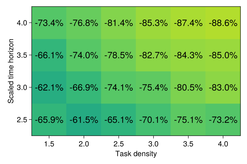
(a) No elementarity, $\mathcal{P}=\mathcal{P}_{\text{all}}$

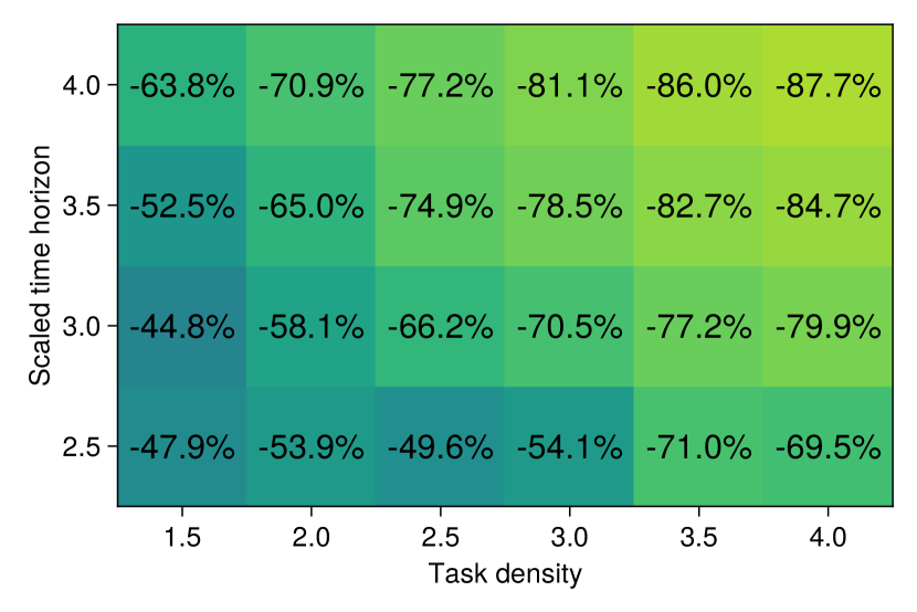
(b) ng-route relaxation, $\mathcal{P}=\mathcal{P}(\mathcal{N})$

Figure 5: Relative speedup of the bi-level label-setting algorithm over the path-based benchmark.

These results show that our bi-level label-setting algorithm results in significant computational improvements against the path-based benchmark. By design, both algorithms generate the same relaxation bounds in the same number of iterations. However, in all instances solved by the path-based benchmark, column generation terminates 50%–90% faster when solving the pricing problem with our bi-level label-setting algorithm. These benefits are highly robust across parameter settings and relaxations. Moreover, our algorithm scales to larger and more complex instances than the benchmark, with full elementarity and 20–24 tasks. These results highlight the impact of the methodology developed in this paper on the computational performance of the pricing problem, hence of the overall column generation algorithm.

Figure 5 shows that the benefits of the bi-level label-setting algorithm are strongest with a larger scaled time horizon and a higher task density. These axes correlate with the number of subpaths per path and the length of each subpath, respectively. In other words, the algorithm is most impactful when each subpath encapsulates multiple tasks and each path encapsulates multiple subpaths. In this regime, the algorithm enables effective decomposition by replacing a large dynamic program with many small ones at the first level and a moderately-sized one at the second level.

Benefits of forward and backward domination criteria for ng-relaxations.

We compare the solution obtained with static and adaptive ng-relaxations to the solutions obtained with no and full elementarity restrictions. The implementations with no elementarity ($\mathcal{P}=\mathcal{P}_{\text{all}}$), full elementarity ($\mathcal{P}=\mathcal{P}_{\text{elem}}$) and static ng-relaxations ($\mathcal{P}=\mathcal{P}(\mathcal{N})$) rely on Steps 1–2 of Algorithm 4. For the static ng-relaxations, we consider ng-neighborhoods $\mathcal{N}$ comprising the closest $N_{\textit{ng}}$ tasks to each node, with $N_{\textit{ng}}=\left\lceil\sqrt[3]{|\mathcal{V}_{T}|}\right\rceil$, $N_{\textit{ng}}=\left\lceil\sqrt{|\mathcal{V}_{T}|}\right\rceil$, and $N_{\textit{ng}}=\lceil|\mathcal{V}_{T}|/3\rceil$. These three settings correspond to small, medium, and large ng-neighborhoods, respectively. The adaptive ng-relaxations start for those same ng-neighborhoods and then apply Steps 1–3 of the algorithm to iteratively tighten the ng-relaxation. Recall, importantly, that static and adaptive ng-relaxations require our forward and backward domination criteria from Section 5.1, as opposed to relying on the basic scheme from Section 4. Table 2 reports the average computational times, relaxation bounds (normalized to the best bound $\overline{\texttt{ERSP}}(\mathcal{P}_{\text{elem}})$) and optimality gaps for each relaxation and three different problem sizes.

Table 2: Computational times of ng- relaxations and adaptive ng- relaxations.

		$n=20$			$n=28$			$n=36$
Method	Size	Time	Relax.	Gap	Time	Relax.	Gap	Time	Relax.	Gap
No elementarity	—	$5.8$s	$0.841$	$53.4$%	$23.0$s	$0.861$	$82.7$%	$51.4$s	$0.892$	$98.7$%
ng-route relaxation	$\lceil\sqrt[3]{|\mathcal{V}_{T}|}\rceil$	$7.3$s	$0.988$	$9.4$%	$42.2$s	$0.990$	$11.2$%	$118.5$s	$0.990$	$14.5$%
	$\lceil\sqrt{|\mathcal{V}_{T}|}\rceil$	$12.2$s	$0.995$	$6.5$%	$71.1$s	$0.994$	$8.8$%	$232.9$s	$0.994$	$12.5$%
	$\lceil|\mathcal{V}_{T}|/3\rceil$	$16.6$s	$0.997$	$6.6$%	$169.7$s	$0.998$	$7.6$%	$1,361.0$s	$0.998$	$9.5$%
adaptive ng-route relaxation	$\lceil\sqrt[3]{|\mathcal{V}_{T}|}\rceil$	$12.0$s	$1.0$	$6.0$%	$869.0$s	$1.0$	$8.0$%	$364.2$s	$1.0$	$10.4$%
	$\lceil\sqrt{|\mathcal{V}_{T}|}\rceil$	$17.1$s	$1.0$	$5.4$%	$111.1$s	$1.0$	$7.5$%	$491.9$s	$1.0$	$10.6$%
	$\lceil|\mathcal{V}_{T}|/3\rceil$	$20.9$s	$1.0$	$5.3$%	$231.8$s	$1.0$	$7.0$%	$1,716.0$s	$1.0$	$9.0$%
Full elementarity	—	$1,943.0$s	$1.0$	$5.4$%	—	—	—	—	—	—

• “—’: instances not completed within 1 hour.

The main observation is that ng-relaxations provide significant accelerations versus the full elementary relaxation, and much stronger relaxations versus the basic relaxation with no elementarity restriction. Notably, the no-elementarity relaxation leaves a very large optimality gap ranging 50–100%; in comparison, the adaptive ng-relaxations improve the relaxation bound by 15% and bring the optimality gaps down to 5–10%. The adaptive ng-relaxations consistently return the strongest possible relaxation in a fraction of the time as compared to the basic column generation scheme on the full elementary relaxation $\overline{\texttt{ERSP}}(\mathcal{P}_{\text{elem}})$. For example, our algorithm terminates in less than 20 seconds with 20 tasks, versus over half an hour when solving $\overline{\texttt{ERSP}}(\mathcal{P}_{\text{elem}})$ directly; and it scales to larger problems on which the $\overline{\texttt{ERSP}}(\mathcal{P}_{\text{elem}})$ relaxation fails to terminate within one hour. The adaptive ng-relaxations yield the tightest possible relaxation bound regardless of the initial ng-neighborhoods. Interestingly, they terminate slightly faster with smaller initial neighborhoods, although the static ng-relaxations get tighter as the ng-neighborhoods become larger. Thus, these results indicates the strength of the adaptive procedure itself to generate strong ng-neighborhoods efficiently. These observations underscore the computational benefits of relying on labels driven by the size of the ng-neighborhoods, as opposed to one label per task with the full elementarity restriction. They also highlight the benefits of our tailored forward and backward domination criteria in our bi-level label-setting algorithm, as compared to relying on the basic criteria from Section 4.

Algorithm scalability.

We conclude these experiments by reporting results of the full solution algorithm (Algorithm 4), incorporating ng-relaxations and lm-SRI cuts—using both sets of forward and backward domination criteria provided in Proposition 5.5 and 5.8. Figure 6 plots the optimality gap and computational times for the ERSP-Hom and the ERSP-Het using the basic column generation scheme (Steps 1–2 of Algorithm 4), the ng-relaxation (Steps 1–3) and the lm-SRI cuts (Steps 1–4).

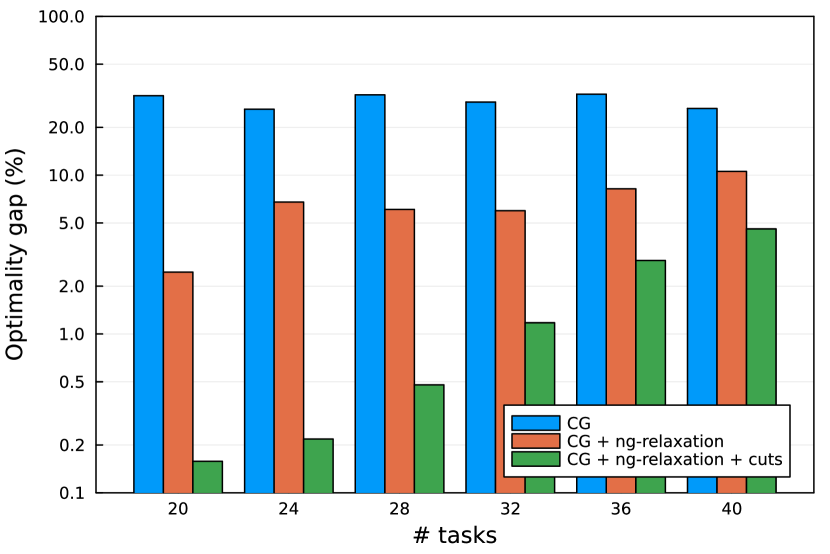
(a) ERSP-Hom: optimality gap

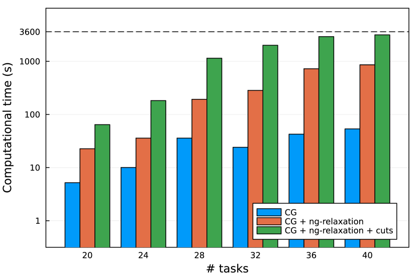
(b) ERSP-Hom: computational time

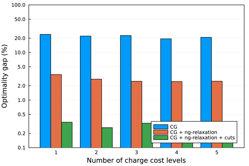
(c) ERSP-Het: optimality gap

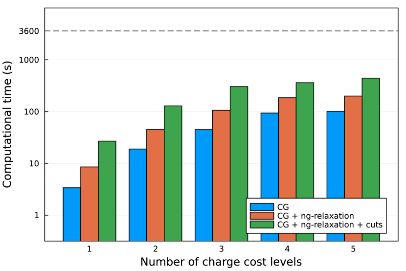
(d) ERSP-Het: computational time

Figure 6: Algorithm performance for ERSP-Hom as a function of the number of tasks and ERSP-Het as a function of the number of charging cost levels (20 tasks), averaged over 20 instances.

The lm-SRI cuts are instrumental in tightening the relaxation of the ERSP (Figure 6(a)). As noted earlier, the elementary relaxation (obtained with the adaptive ng-relaxations) leaves an optimality gap of 5–10%, but the lm-SRI cuts reduce the gap to 0.2–5%. As expected, these improvements come at the cost of longer computational times (Figure 6(b)), since the pricing problem uses an extra domination label per cut (Equation (45)). Still, the algorithm returns provably near-optimal solutions (within 5% of the optimum) in manageable computational times (within one hour) for problems with up to 40 task nodes. The algorithm returns consistent optimality gaps—if anything, slightly lower ones—as charging costs become more heterogeneous across charging stations (Figure 6(c)). As expected, more charging cost levels increase computational times (Figure 6(d)) due to the extra domination labels (Proposition 4.15). Nonetheless, the overall stability in computational times indicates our algorithm’s ability to handle heterogeneous charging costs in the ESRP, with similarly high-quality solutions and only slightly longer computational times.

Finally, Figure 7 shows that our methodology results in a Pareto improvement over state-of-the-art methods for the ERSP-Hom: better primal solutions and stronger relaxation bounds in shorter computational times. The state-of-the-art benchmark considered here combines the path-based label-setting algorithm from Desaulniers et al. (2016) (already considered in Table 1) with adaptive ng-relaxations and lm-SRI cuts. Note that the ng-relaxations and lm-SRI cuts only require the forward domination criteria in the benchmark, as opposed to forward and backward domination criteria in our bi-level label-setting algorithm. In medium-scale instances (Figure 7(a)), our algorithm achieves a tight optimality gap in seconds to minutes, versus minutes to hours for the benchmark. In large-scale instances (Figure 7(b)), neither method returns an optimal solution; still, our method yields a stronger primal solution and a stronger relaxation bound after 10 minutes than the benchmark after one hour, on average. Moreover, our algorithm exhibits lower performance variability across instances, which also enhances the reliability of the overall methodology.

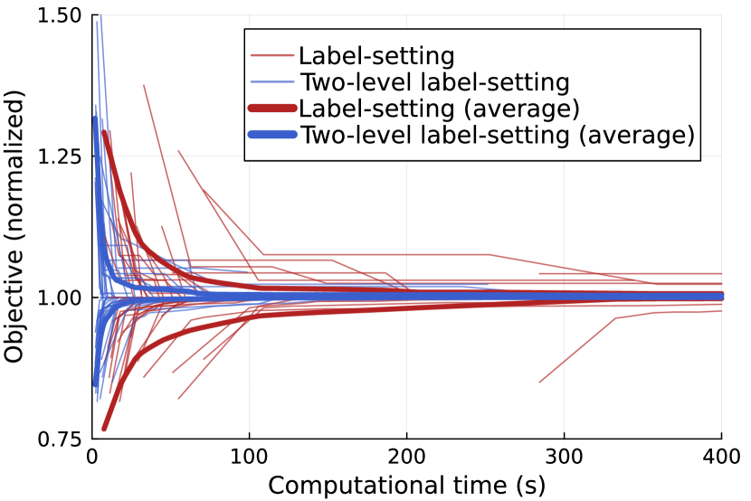
(a) 20 tasks

(b) 32 tasks

Figure 7: Comparison of the bi-level label-setting methodology developed in this paper to a state-of-the-art path-based benchmark for the ERSP-Hom, both with adpative ng-relaxations and lm-SRI cuts.

In summary, the methodology developed in this paper provides two major contributions: (i) it scales to large and otherwise-intractable ERSP-Hom instances, yielding win-win-win outcomes reflected in higher-quality solutions and tighter relaxations in faster computational times; and (ii) it provides the first solution approach to handle heterogeneous charging costs in the ERSP-Het.

Practical impact.

We conclude by assessing the practical benefits of the optimization methodology against practical benchmarks that could be more easily implemented in practice. We first evaluate the impact of jointly optimizing routing-scheduling and charging decisions. Figure 8(a) reports the percent-wise improvements of our solution against a sequential route-then-charge benchmark for the ERSP-Hom. This benchmark first optimizes routing-scheduling decisions without consideration for charging requirements (using traditional routing-scheduling algorithms), and then appends charging decisions to ensure sufficient battery levels. Results show that the integrated optimization approach can yield up to 8% reductions in operating costs. The gains become smaller as the scale of the problem increases due to the difficulty to find near-optimal solutions in the integrated problem. Nonetheless, the benefits of integrated optimization can be highly significant, especially under low task density—that is, when charging decisions become more critical.

Next, we evaluate the impact of capturing heterogeneous charging costs in the ERSP-Het—an important feature in practice, as discussed earlier (Basma et al. 2023). Figure 8(b) compares the solution to one obtained with the ERSP-Hom model, using existing algorithms. Results show that the ERSP-Het solution results in 5-20% reductions in charging costs. These benefits are again most significant under low density. Moreover, they also increase as the number of different charge levels gets larger, in which case accounting for heterogeneous charging costs becomes more important. We also observe non-increasing returns, suggesting that significant savings in charging costs can even be achieved with a small number of charging cost levels.

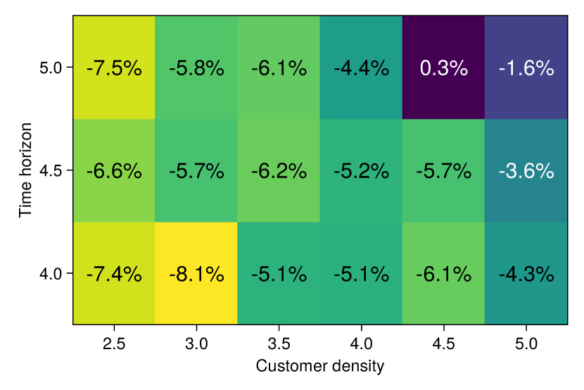
(a) Benefits of ESRP-Hom over route-then-charge

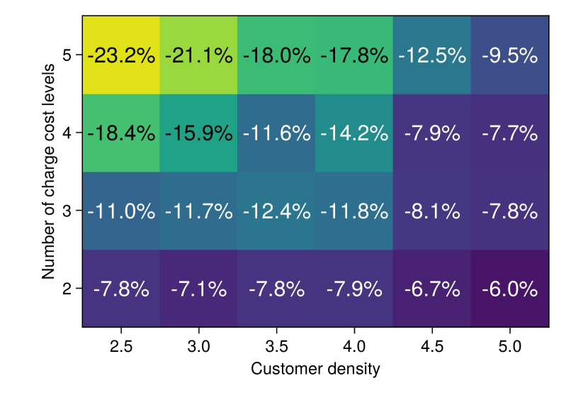
(b) Benefits of ESRP-Het over ERSP-Hom

Figure 8: Benefits of integrated routing-scheduling and charging optimization against practical benchmarks.

Altogether, these findings underscore that electrification does not merely require downstream adjustments in business-as-usual operations; instead, it necessitates comprehensive re-optimization to create synergistic routing, scheduling and charging operations. Dedicated optimization tools such as the one developed in this paper can therefore yield strong performance improvements in electrified operations, both in economic terms—reduction in operating costs—and in sustainability terms—adoption of electrification technologies with more limited environmental footprint.

7 Conclusion

This paper considers an electric routing-scheduling problem, which augments canonical vehicle routing and scheduling problems with electrified operations. The problem jointly optimizes routing-scheduling and charging decisions, with flexibility regarding where, when and for how long to charge. We formulate it as a semi-infinite optimization problem given the infinite number of charging decisions. We develop a column generation methodology based on a bi-level label-setting algorithm that separates routing-scheduling and charging decisions in the pricing problem. Specifically, a first-level procedure generates subpaths between charging decisions, and a second-level procedure combines subpaths to reconstruct full paths. The methodology can accommodate, via extra labels, new modeling features (e.g., heterogeneous charging costs) and recent advances in routing algorithms (e.g., ng-relaxations and lm-SRI cuts). We formally prove that the resulting column generation algorithm terminates in an finite number of iterations with exact relaxation bounds.

Extensive computational experiments yield three main takeaways. First, the bi-level label-setting algorithm achieves significant speedups as compared to traditional path-based label-setting methods, and can solve tight relaxations in manageable computational times. In turn, our methodology scales to otherwise-intractable problems, by returning higher-quality solutions in faster computational times than state-of-the-art benchmarks. Second, this paper provides the first exact methodology to handle heterogeneous charging costs in electric routing-scheduling optimization. Third, the methodology can provide strong practical benefits, with significant reductions in operating costs and a concomitant reduction in carbon emissions. At a time where decarbonization goals require fast and large-scale electrification, these benefits can magnify the adoption and impact of electrified technologies across the logistics, service and manufacturing industries.

Electronic Companion

8 Path-based label-setting benchmark

We outline the path-based label-setting procedure for EVRP-Hom, which we use as a benchmark in the paper. It is also useful to introduce some techniques used in our bi-level label-setting procedure. Proofs from this section are omitted for conciseness, because they are similar to (and much simpler than) those of our algorithm, and they follow standard arguments in vehicle routing.

General label-setting benchmark.

Recall that a path starts from the source at the beginning of the planning horizon with full charge, and ends at the sink by the end of the planning horizon, while maintaining a non-negative level of charge throughout (Definition 3.1). The pricing problem seeks a path of minimal reduced cost, given in Equation (10).

Definition 8.1 (Extensions of partial paths)

Consider a feasible partial path $p\in\mathcal{P}^{\circ}$ with node sequence $\{n_{0},\cdots,n_{m}\}$ such that $n_{\text{end}}^{s}=n_{m}\notin\mathcal{V}_{D}$, and with charging time sequence $C(p)=\set{\tau_{k}\mid k\in[m-1],n_{k}\in\mathcal{V}_{R}}$. An extension $a$ of $p$ comprises an arc $(n_{m},n_{m+1})\in\mathcal{A}$ and a charging time $\tau_{m}\geq 0$ $n_{m}\in\mathcal{V}_{R}$. The extension is feasible if $t^{s}+t(n_{m},n_{m+1})\leq T$ and $b^{s}+b(n_{m},n_{m+1})\leq B$ if $n_{m}\notin\mathcal{V}_{R}$; and if $t^{s}+\tau_{m}+t(n_{m},n_{m+1})\leq T$ and $\min(b^{s}+\tau_{m},B)-b(n_{m},n_{m+1})\geq 0$ if $n_{m}\in\mathcal{V}_{R}$. We denote by $p\oplus a$ the extended partial path defined by node sequence $U(p\oplus a)=\{n_{0},\cdots,n_{m},n_{m+1}\}$ and charging time sequence $C(p\oplus a)=\set{\tau_{k}}{k\in[m],n_{k}\in\mathcal{V}_{R}}$.

Definition 8.2 (Reduced cost contribution)

Consider partial path $p\in\mathcal{P}^{\circ}$ with node sequence $\{n_{0},\cdots,n_{m}\}$ such that $n_{\text{end}}^{s}=n_{m}\notin\mathcal{V}_{D}$, and with charging time sequence $C(p)=\set{\tau_{k}\mid k\in[m-1],n_{k}\in\mathcal{V}_{R}}$. Given dual variables $\bm{\kappa}$, $\bm{\mu}$, and $\bm{\nu}$, its reduced cost contribution is:

$$\widehat{c}^{p} =\sum_{l=0}^{m-1}\left(c(n_{l},n_{l+1})+\mathbb{1}\left(n_{l}\in\mathcal{V}_{R}\right)\cdot\delta\cdot\tau_{l}-\mathbb{1}\left(n_{l+1}\in\mathcal{V}_{T}\right)\nu_{n_{l+1}}\right)-\kappa_{n_{0}}-\mathbb{1}\left(n_{m}\in\mathcal{V}_{D}\right)\mu_{n_{m}}$$

The main difference between the extension of a path and the extension of a subpath is that the former encapsulates a charging decision if the current node is a charging station, whereas the latter is restricted to routing-scheduling decisions. Similarly, the reduced cost contribution of a partial path includes the cost of charging, whereas this cost component is moot in a partial subpath.

We define necessary conditions for path-based domination criteria in Proposition 8.2. We also complement it with path-based termination criteria in Property 8.2. Proposition 8.3 provides domination and non-domination criteria that satisfy these properties.

[Domination criteria for paths] $(\mathrm{D}\left(\cdot\right),\mathrm{ND}\left(\cdot\right),\mathcal{P})$ must satisfy:

1. For feasible partial paths $p_{1},p_{2}\in\mathcal{P}^{\circ}$ such that $p_{1}\succeq p_{2}$, and an extension $a\in\mathcal{A}$ of $p_{1}$ and $p_{2}$, either (a) $p_{2}\oplus a\notin\mathcal{P}^{\circ}$, or (b) $p_{1}\oplus a\in\mathcal{P}^{\circ}$, $p_{2}\oplus a\in\mathcal{P}^{\circ}$, and $p_{1}\oplus a\succeq p_{2}\oplus a$.

[Termination criteria for paths] $(\mathrm{D^{s}}\left(\cdot\right),\mathrm{ND^{s}}\left(\cdot\right),\mathcal{S})$ must satisfy:

1. One component of $\mathrm{D}\left(\cdot\right)$ captures the reduced cost contribution of partial path $s\in\mathcal{P}^{\circ}$.

2. One component of $\mathrm{D}\left(\cdot\right)$ is nonnegative, strictly monotone, and bounded by a constant.

Proposition 8.3

The following criteria satisfy Property 8.2 and 8.2 for EVRP-Hom:

$$\text{For $\mathcal{P}=\mathcal{P}_{\text{all}}$:}\quad\mathrm{ND}\left(p\right) =(n_{\text{start}}^{p},n_{\text{end}}^{p}), \mathrm{D}\left(p\right)=(\widehat{c}^{p},t_{\text{end}}^{p},-b_{\text{end}}^{p}),$$

$$\text{For $\mathcal{P}=\mathcal{P}_{\text{elem}}$:}\quad\mathrm{ND}\left(p\right) =(n_{\text{start}}^{p},n_{\text{end}}^{p}), \mathrm{D}\left(p\right)=(\widehat{c}^{p},t_{\text{end}}^{p},-b_{\text{end}}^{p},\{\gamma_{i}^{p}\}_{i\in\mathcal{V}_{T}})).$$

An extension of path $p$ with arc $a=(n_{\text{end}}^{p},n_{\text{next}})$ and charging time $\tau$ (if applicable) yields:

$$\mathrm{ND}\left(p\oplus a\right) =(n_{\text{start}}^{p},n_{\text{next}})$$

$$\widehat{c}^{p\oplus a} =\widehat{c}^{p}+c(n_{\text{end}}^{p},n_{\text{next}})+\mathbb{1}\left(n_{\text{end}}^{p}\in\mathcal{V}_{R}\right)\cdot\delta\cdot\tau$$

$$\quad-\mathbb{1}\left(n_{\text{next}}\in\mathcal{V}_{T}\right)\nu_{n_{\text{next}}}-\mathbb{1}\left(n_{\text{next}}\in\mathcal{V}_{D}\right)\mu_{n_{\text{next}}}$$

$$t_{\text{end}}^{p\oplus a} =t_{\text{end}}^{p}+\mathbb{1}\left(n_{\text{end}}^{p}\in\mathcal{V}_{R}\right)\cdot\tau+t(n_{\text{end}}^{p},n_{\text{next}})$$

$$-b_{\text{end}}^{p\oplus a} =\max\Big{\{}-b_{\text{end}}^{p}-\mathbb{1}\left(n_{\text{end}}^{p}\in\mathcal{V}_{R}\right)\cdot\tau,\ -B\Big{\}}+b(n_{\text{end}}^{p},n_{\text{next}})$$

$$\gamma_{i}^{p\oplus a} =\gamma_{i}^{p}+\mathbb{1}\left(n_{\text{next}}=i\right),\ \forall\ i\in\mathcal{V}_{T}\quad\text{(with elementarity constraints)}$$

Algorithm 5 presents the path-based label-setting algorithm. This algorithm is similar to Algorithm 2, except that it starts and ends at a depot, and that the partial path extensions can visit charging stations in-between. As in the case of subpaths, elementarity (or relaxations thereof) of feasible paths $p\in\mathcal{P}\subset\mathcal{P}_{\text{all}}$ can be imposed on the partial paths $p^{\prime}\in\mathcal{P}^{\circ}\subset\mathcal{P}_{\text{all}}^{\circ}$. Theorem 8.4 shows that Algorithm 5 yields the set of non-dominated paths $\tilde{\mathcal{P}}$ with respect to path set $\mathcal{P}$, as long as the non-domination and domination criteria satisfy Properties 8.2 and 8.2.

Algorithm 5 FindNonDominatedPaths$\big{(}\mathrm{D}\left(\cdot\right),\mathrm{ND}\left(\cdot\right),\mathcal{P}^{\circ}\big{)}$.

Initialization: $\mathcal{P}_{\text{gen}}=\emptyset$; store in $\mathcal{P}_{\text{queue}}$ all single-node partial paths starting at nodes $i\in\mathcal{V}_{D}$.

Iterate between Steps 1-3.

• Step 1. Select $p\in\argmin\set{\mathrm{D}_{2}\left(p\right):p\in\mathcal{P}_{\text{queue}}}$. Remove $p$ from $\mathcal{P}_{\text{queue}}$ and add it to $\mathcal{P}_{\text{gen}}$.

  If $p$ is a path, go to Step 3. Else, go to Step 2.

• Step 2. For each extension $a$ of $p$, denoting $p_{\text{next}}:=p\oplus a$:

  1. If $p_{\text{next}}\notin\mathcal{P}^{\circ}$, or if any $p^{\prime}\in\mathcal{P}_{\text{queue}}\cup\mathcal{P}_{\text{gen}}$ is such that $p^{\prime}\succeq p_{\text{next}}$, continue.

  2. Otherwise, remove any $p^{\prime}\in\mathcal{P}_{\text{queue}}$ such that $p_{\text{next}}\succeq p^{\prime}$, and add $p_{\text{next}}$ to $\mathcal{P}_{\text{queue}}$.

• Step 3. If $|\mathcal{P}_{\text{queue}}|=0$, STOP: return solution $\mathcal{P}_{\text{result}}:=\set{p\in\mathcal{P}_{\text{gen}}:p\text{ is a path}}$.

Theorem 8.4

If $(\mathrm{D}\left(\cdot\right),\mathrm{ND}\left(\cdot\right),\mathcal{P})$ satisfy Property 8.2 and 8.2, Algorithm 5 returns the set $\tilde{\mathcal{P}}$ of non-dominated paths with respect to $\mathcal{P}$. If $\mathcal{P}_{\text{neg}}\neq\emptyset$, then $\mathcal{P}_{\text{neg}}\cap\tilde{\mathcal{P}}\neq\emptyset$.

Algorithm 5 involves infinitely many possible extensions of any partial path ending at a charging station, due to the infinitely-sized of charging times. Accordingly, Theorem 8.4 establishes the exactness of the algorithm upon termination but does not guarantee finite convergence—unlike Theorem 4.16. Any practical implementation of Algorithm 5 must therefore specify a rule to handle the infinite number of possible extensions at charging stations (see, e.g. Desaulniers et al. 2016). Our paper proposes an alternative approach via a two-level label-setting algorithm that generates subpaths from and to charging actions and then combines them into full paths.

9 Proofs in Section 4

Properties 4.4 and 4.2 are necessary conditions to extend domination patterns along subpaths and subpath sequences. We complement them with technical conditions that are necessary for termination.

[Termination criteria for subpaths] $(\mathrm{D^{s}}\left(\cdot\right),\mathrm{ND^{s}}\left(\cdot\right),\mathcal{S})$ must satisfy:

1. One component of $\mathrm{D^{s}}\left(\cdot\right)$ captures the reduced cost contribution $\widehat{c}^{s}$ of partial subpath $s\in\mathcal{S}$.

2. One component of $\mathrm{D^{s}}\left(\cdot\right)$ is nonnegative, strictly monotone, and bounded by a constant.

[Termination criteria for subpath sequences] $(\mathrm{D^{s}}\left(\cdot\right),\mathrm{ND^{s}}\left(\cdot\right),\mathcal{S})$ and $(\mathrm{D}\left(\cdot\right),\mathrm{ND}\left(\cdot\right),\mathcal{P})$ must satisfy:

1. One component of $\mathrm{D}\left(\cdot\right)$ captures the reduced cost contribution $\widehat{c}^{p_{\text{min}}\left(\sigma\right)}$ of the minimal path $p_{\text{min}}\left(\sigma\right)$. Moreover, if $\sigma_{1}\succeq\sigma_{2}\in{\bm{\mathcal{S}}^{\circ}}$, then $\widehat{c}^{p_{\text{min}}\left(\sigma_{1}\right)}\leq\widehat{c}^{p_{\text{min}}\left(\sigma_{2}\right)}$.

2. One component of $\mathrm{D}\left(\cdot\right)$ is nonnegative, strictly monotone, and bounded by a constant.

Proof of Lemma 4.8.

Let $p\in\mathcal{P}$ be a feasible path, with complete subpath sequence $\sigma=\{s_{1},\dots,s_{k}\}$ and charging time sequence $\{\tau_{1},\dots,\tau_{k-1}\}$. For $j\in\{1,\cdots,k\}$, let subpath $s_{j}$ have node sequence $U(s_{j})=\{n_{j,0},\dots,n_{j,m_{j}}\}$. (For consistency we must have $n_{j,m_{j}}=n_{j+1,0}$ for all $j\in\{1,\cdots,k-1\}$). By definition of a path and a subpath, we have $n_{1,0},n_{k,m_{k}}\in\mathcal{V}_{D}$, $n_{1,m_{1}},n_{2,0},\dots,n_{k-1,m_{k-1}},n_{k,0}\in\mathcal{V}_{R}$, and $n_{j,l}\in\mathcal{V}_{T}$ for all $j\in\{1,\cdots,k\},l\in\{1,\dots,m_{j}-1\}$. Therefore, the reduced cost of $p$ is:

$$\overline{c}^{p} =c^{p}-\sum_{j\in\mathcal{V}_{D}}\mathbb{1}\left(n_{\text{start}}^{p}=j\right)\kappa_{j}-\sum_{j\in\mathcal{V}_{D}}\mathbb{1}\left(n_{\text{end}}^{p}=j\right)\mu_{j}-\sum_{i\in\mathcal{V}_{T}}\gamma_{i}^{p}\nu_{i}\quad\text{(by Equation~{}\eqref{eq:RC})}$$

$$=\sum_{j=1}^{k}\sum_{l=0}^{m_{j}-1}c(n_{j,l},n_{j,l+1})+\sum_{j=1}^{k-1}\delta(n_{\text{end}}^{s_{j}})\cdot\tau_{j}-\kappa_{n_{1,0}}-\mu_{n_{k,m_{k}}}-\sum_{j=1}^{k}\sum_{l=0}^{m_{j}-1}\nu_{n_{j,l+1}}\quad\text{(by Definition~{}\ref{def:path})}$$

$$=\sum_{j=1}^{k}\left[\sum_{l=0}^{m_{j}-1}\left(c(n_{j,l},n_{j,l+1})-\mathbb{1}\left(n_{j,l+1}\in\mathcal{V}_{T}\right)\nu_{n_{j,l+1}}\right)-\mathbb{1}\left(j=1\right)\kappa_{n_{j,0}}-\mathbb{1}\left(j=k\right)\mu_{n_{j,m_{j}}}\right]+\sum_{j=1}^{k-1}\delta(n_{\text{end}}^{s_{j}})\cdot\tau_{j}$$

$$=\sum_{j=1}^{k}\widehat{c}^{s_{j}}+\sum_{j=1}^{k-1}\delta(n_{\text{end}}^{s_{j}})\cdot\tau_{j}\quad\text{(by Definition~{}\ref{def:reduced_cost_partial_subpath})}$$

$$=\widehat{c}^{p}\hfill\Halmos$$

Proof of Proposition 4.5.

We first prove Equations (14)–(18). Let $s$ be a partial subpath with node sequence $\{n_{0},\dots,n_{m}\}$ and $a=(n_{\text{end}}^{s},n_{\text{next}})=(n_{m},n_{m+1})$. In particular, $n_{m}\notin\mathcal{V}_{D}$. We have:

$$\mathrm{ND^{s}}\left(s\oplus a\right) =(n_{0},n_{m+1})=(n_{\text{start}}^{s},n_{\text{next}}).$$

$$\widehat{c}^{s\oplus a} =\sum_{\ell=0}^{m-1}\left(c(n_{\ell},n_{\ell+1})-\mathbb{1}\left(n_{\ell+1}\in\mathcal{V}_{T}\right)\nu_{n_{\ell+1}}\right)-\mathbb{1}\left(n_{0}\in\mathcal{V}_{D}\right)\kappa_{n_{0}}$$

$$\quad+c(n_{m},n_{m+1})-\mathbb{1}\left(n_{m+1}\in\mathcal{V}_{T}\right)\nu_{n_{m+1}}-\mathbb{1}\left(n_{m+1}\in\mathcal{V}_{D}\right)\mu_{n_{m+1}}$$

$$=\widehat{c}^{s}+c(n_{\text{end}}^{s},n_{\text{next}})-\mathbb{1}\left(n_{\text{next}}\in\mathcal{V}_{T}\right)\nu_{n_{\text{next}}}-\mathbb{1}\left(n_{\text{next}}\in\mathcal{V}_{D}\right)\mu_{n_{\text{next}}}.$$

$$t^{s\oplus a} =\sum_{\ell=0}^{m}t(n_{\ell},n_{\ell+1})=\sum_{\ell=0}^{m-1}t(n_{\ell},n_{\ell+1})+t(n_{\text{end}}^{s},n_{\text{next}})=t^{s}+t(n_{\text{end}}^{s},n_{\text{next}}).$$

$$b^{s\oplus a} =\sum_{\ell=0}^{m}b(n_{\ell},n_{\ell+1})=\sum_{\ell=0}^{m-1}b(n_{\ell},n_{\ell+1})+b(n_{\text{end}}^{s},n_{\text{next}})=b^{s}+b(n_{\text{end}}^{s},n_{\text{next}}).$$

$$\gamma_{i}^{s\oplus a} =|\Set{n\in U(s\oplus a)}{n=i}|=|\Set{n\in U(s)}{n=i}|+\mathbb{1}\left(n_{\text{next}}=i\right)=\gamma_{i}^{s}+\mathbb{1}\left(n_{\text{next}}=i\right).$$

Let us prove that $\mathrm{D^{s}}\left(\cdot\right)$ and $\mathrm{ND^{s}}\left(\cdot\right)$ satisfy Properties 4.2 and 9.

Property 4.4: Let $s_{1},s_{2}\in\mathcal{S}_{\text{all}}^{\circ}$ be partial subpaths starting in $n_{\text{start}}$ and ending in $n_{\text{end}}$ with $s_{1}\succeq_{s}s_{2}$, i.e., $\mathrm{ND^{s}}\left(s_{1}\right)=\mathrm{ND^{s}}\left(s_{2}\right)$ and $\mathrm{D^{s}}\left(s_{1}\right)\leq\mathrm{D^{s}}\left(s_{2}\right)$ component-wise. Let $a=(n_{\text{end}},n_{\text{next}})$ be an arc extension of $s_{1}$ and $s_{2}$. First, $\mathrm{ND^{s}}\left(s_{1}\oplus a\right)=\mathrm{ND^{s}}\left(s_{2}\oplus a\right)=(n_{\text{start}},n_{\text{next}})$. Suppose that $s_{2}\oplus a\in\mathcal{S}_{\text{all}}^{\circ}$, i.e., $t^{s_{2}\oplus a}\in[0,T]$ and $b^{s_{2}\oplus a}\in[0,B]$. We show that $\mathrm{D^{s}}\left(s_{1}\oplus a\right)\leq\mathrm{D^{s}}\left(s_{2}\oplus a\right)$, using Definitions 4.1 and 4.3:

$$\widehat{c}^{s_{1}\oplus a} =\widehat{c}^{s_{1}}+c(n_{\text{end}},n_{\text{next}})-\mathbb{1}\left(n_{\text{next}}\in\mathcal{V}_{T}\right)\nu_{n_{\text{next}}}-\mathbb{1}\left(n_{\text{next}}\in\mathcal{V}_{D}\right)\mu_{n_{\text{next}}}$$

$$\leq\widehat{c}^{s_{2}}+c(n_{\text{end}},n_{\text{next}})-\mathbb{1}\left(n_{\text{next}}\in\mathcal{V}_{T}\right)\nu_{n_{\text{next}}}-\mathbb{1}\left(n_{\text{next}}\in\mathcal{V}_{D}\right)\mu_{n_{\text{next}}}=\widehat{c}^{s_{2}\oplus a}$$

$$t^{s_{1}\oplus a} =t^{s_{1}}+t(n_{\text{end}},n_{\text{next}})\leq t^{s_{2}}+t(n_{\text{end}},n_{\text{next}})=t^{s_{2}\oplus a}$$

$$b^{s_{1}\oplus a} =b^{s_{1}}+b(n_{\text{end}},n_{\text{next}})\leq b^{s_{2}}+b(n_{\text{end}},n_{\text{next}})=b^{s_{2}\oplus a}$$

$$\gamma_{i}^{s_{1}\oplus a}=\gamma_{i}^{s_{1}}+\mathbb{1}\left(n_{\text{next}}=i\right)\leq\gamma_{i}^{s_{2}}+\mathbb{1}\left(n_{\text{next}}=i\right)=\gamma_{i}^{s_{2}\oplus a}$$ (with elementarity)

Moreover, $s_{1}\oplus a$ is a feasible partial subpath because:

$$t^{s_{2}\oplus a}\in[0,T]\text{ and } 0\leq t^{s_{1}\oplus a}\leq t^{s_{2}\oplus a} \implies t^{s_{1}\oplus a}\in[0,T]$$

$$b^{s_{2}\oplus a}\in[0,B]\text{ and } 0\leq b^{s_{1}\oplus a}\leq b^{s_{2}\oplus a} \implies b^{s_{1}\oplus a}\in[0,B]$$

$$\gamma_{i}^{s_{1}\oplus a}\leq\gamma_{i}^{s_{2}\oplus a}\leq 1 \implies\gamma_{i}^{s_{1}\oplus a}\in\{0,1\}$$ (with elementarity)

Property 9: The first component captures the reduced cost contribution. The second component captures the time; it is non-negative, strictly monotone because $\min\{t_{i,j}:(i,j)\in\mathcal{E}\}>0$, and bounded above by $T$.

Proof of Proposition 4.12.

We first introduce some definitions pertaining to subpath sequences:

Definition 9.1

For a subpath sequence $\sigma$, we define its node sequence $U(\sigma)$ as the node sequence of the concatenation of $s_{1},\dots,s_{m}$, without double-counting the charging stations:

$$U(\sigma\oplus s)=U(\sigma)\cup\left(U(s)\setminus\{n_{\text{start}}^{s}\}\right)$$

We first prove Equations (22)–(26). Consider a subpath sequence $\sigma=\{s_{1},\dots,s_{m}\}\in\SS$ and an extension $s\in\mathcal{S}$. We have:

$$\mathrm{ND}\left(\sigma\oplus s\right) =(n_{\text{start}}^{\sigma\oplus s},n_{\text{end}}^{\sigma\oplus s})=(n_{\text{start}}^{\sigma},n_{\text{end}}^{s}).$$

$$\forall\ i\in\mathcal{V}_{T}, \gamma_{i}^{\sigma\oplus s} =|\Set{n\in U(\sigma\oplus s)}{n=i}|$$

$$=|\Set{n\in U(\sigma)}{n=i}|+|\Set{n\in(U(s)\setminus\{n_{\text{start}}^{s}\})}{n=i}|$$

$$=\gamma_{i}^{\sigma}+\gamma_{i}^{s}.$$

This proves Equations (22) and (26). Equations (23)–(25) are due the following lemma.

Lemma 9.2

For ERSP-Hom, given a feasible subpath sequence $\{s_{1},\dots,s_{m}\}$, define the subsequences $\sigma_{j}=\{s_{1},\dots,s_{j}\}$. There exists a sequence of charging times $\{\tau_{1},\dots,\tau_{m-1}\}$ such that $\{\tau_{1},\dots,\tau_{j-1}\}$ is the charging sequence of $p_{\text{min}}\left(\sigma_{j}\right)$ for all $j\in\{1,\dots,m\}$, defined by:

$$\tau_{j} =\left(b^{s_{j+1}}-\left(B-\sum_{i=1}^{j}b^{s_{i}}\right)^{+}\right)^{+}$$

Therefore, $p_{\text{min}}\left(\sigma_{j}\right)$ is the path with reduced cost contribution $\widehat{c}^{p_{\text{min}}\left(\sigma_{j}\right)}$, ending at time $t_{\text{end}}^{p_{\text{min}}\left(\sigma_{j}\right)}$ with charge $b_{\text{end}}^{p_{\text{min}}\left(\sigma_{j}\right)}$ with:

$$\widehat{c}^{p_{\text{min}}\left(\sigma_{j}\right)} =\sum_{i=1}^{j}\widehat{c}^{s_{i}}+\delta\cdot\left(\sum_{i=1}^{j}b^{s_{i}}-B\right)^{+}$$ (52)

$$t_{\text{end}}^{p_{\text{min}}\left(\sigma_{j}\right)} =\sum_{i=1}^{j}t^{s_{i}}+\left(\sum_{i=1}^{j}b^{s_{i}}-B\right)^{+}$$ (53)

$$b_{\text{end}}^{p_{\text{min}}\left(\sigma_{j}\right)} =\left(B-\sum_{i=1}^{j}b^{s_{i}}\right)^{+}$$ (54)

Proof 9.3

Proof of Lemma 9.2. To determine $p_{\text{min}}\left(\sigma_{m}\right)$ for the full subpath sequence, we need to determine a sequence of charging times $\{\tau_{1},\dots,\tau_{m-1}\}$ such that all intermediate partial paths have sufficient charge. From Definition 4.10, this can be formulated as the following optimization problem:

$$\min_{\tau_{1},\dots,\tau_{m-1}}\quad \sum_{i=1}^{m-1}\delta\cdot\tau_{i}$$

s.t. $$\sum_{i=1}^{j+1}b^{s_{i}}-B\ \leq\ \sum_{i=1}^{j}\tau_{i}\ \leq\ \sum_{i=1}^{j}b^{s_{i}} \forall\ j\in\{1,\cdots,m-1\}$$

$$\tau_{i}\geq 0, \forall\ i\in\{1,\cdots,m-1\}$$

The optimal objective value must be at most $\left(\sum_{i=1}^{m}b^{s_{i}}-B\right)^{+}$ (implied by the last constraint). This objective value is attainable by the solution:

$$\sum_{i=1}^{j}\tau_{i}=\left(\sum_{i=1}^{j+1}b^{s_{i}}-B\right)^{+},\ \forall\ j\in\{1,\cdots,m-1\}$$

This implies, for all $j\in\{1,\cdots,m-1\}$:

$$\tau_{j} =\left(\sum_{i=1}^{j+1}b^{s_{i}}-B\right)^{+}-\left(\sum_{i=1}^{j}b^{s_{i}}-B\right)^{+}$$

$$=\max\{b^{s_{j+1}}-x-\left(-x\right)^{+},-\left(-x\right)^{+}\} x=B-\sum_{i=1}^{j}b^{s_{i}}$$ with

$$=\max\{b^{s_{j+1}}-\left(x\right)^{+},-\left(-x\right)^{+}\}$$

$$=\max\{b^{s_{j+1}}-\left(x\right)^{+},0\} x\geq 0 x<0$$ (considering the cases and )

$$=\left(b^{s_{j+1}}-\left(B-\sum_{i=1}^{j}b^{s_{i}}\right)^{+}\right)^{+}$$

For each $j\in\{1,\cdots,m\}$, the partial solution $\{\tau_{1},\dots,\tau_{j-1}\}$ is also optimal for the optimization problem defined by $p_{\text{min}}\left(\sigma_{j}\right)$. Since the total amount charged is $\sum_{i=1}^{j-1}\tau_{i}=\left(\sum_{i=1}^{j}b^{s_{i}}-B\right)^{+}$, this proves Equations (52)–(53). For Equation (54), we have by recursion:

$$b_{\text{end}}^{p_{\text{min}}\left(\sigma_{j}\right)} =b_{\text{end}}^{p_{\text{min}}\left(\sigma_{j-1}\right)}+\tau_{j-1}-b^{s_{j}}$$

$$=\dots$$

$$=B-b^{s_{1}}+\tau_{1}-b^{s_{2}}+\dots+\tau_{j-1}-b^{s_{j}}$$

$$=B-\sum_{i=1}^{j}b^{s_{i}}+\sum_{i=1}^{j-1}\tau_{i}$$

$$=B-\sum_{i=1}^{j}b^{s_{i}}+\left(\sum_{i=1}^{j}b^{s_{i}}-B\right)^{+}$$

$$=\left(B-\sum_{i=1}^{j}b^{s_{i}}\right)^{+}$$

This completes the proof of the lemma.

We now verify Equations (23)–(25). Letting $\sigma=\{s_{1},\dots,s_{m}\}$ be extended by $s_{m+1}$, and defining $\tau=\left(b^{s_{m+1}}-b_{\text{end}}^{p_{\text{min}}\left(\sigma\right)}\right)^{+}$,

$$\tau =\left(b^{s_{m+1}}-b_{\text{end}}^{p_{\text{min}}\left(\sigma\right)}\right)^{+}$$

$$=\left(b^{s_{m+1}}-\left(B-\sum_{i=1}^{m}b^{s_{i}}\right)^{+}\right)^{+}\quad\text{(by Lemma~{}\ref{lem:minpath_ersphom})}$$

$$=\left(\sum_{i=1}^{m+1}b^{s_{i}}-B\right)^{+}-\left(\sum_{i=1}^{m}b^{s_{i}}-B\right)^{+}$$

Therefore:

$$\widehat{c}^{p_{\text{min}}\left(\sigma\oplus s_{m+1}\right)} =\sum_{i=1}^{m+1}\widehat{c}^{s_{i}}+\delta\cdot\left(\sum_{i=1}^{m+1}b^{s_{i}}-B\right)^{+}\quad\text{(by Lemma~{}\ref{lem:minpath_ersphom})}$$

$$=\sum_{i=1}^{m}\widehat{c}^{s_{i}}+\delta\cdot\left(\sum_{i=1}^{m}b^{s_{i}}-B\right)^{+}+\delta\cdot\tau+\widehat{c}^{s_{m+1}}$$

$$=\widehat{c}^{p_{\text{min}}\left(\sigma\right)}+\delta\cdot\tau+\widehat{c}^{s_{m+1}}\quad\text{(by Lemma~{}\ref{lem:minpath_ersphom})}$$

$$t_{\text{end}}^{p_{\text{min}}\left(\sigma\oplus s_{m+1}\right)} =\sum_{i=1}^{m+1}t^{s_{i}}+\left(\sum_{i=1}^{m+1}b^{s_{i}}-B\right)^{+}\quad\text{(by Lemma~{}\ref{lem:minpath_ersphom})}$$

$$=\sum_{i=1}^{m}t^{s_{i}}+\left(\sum_{i=1}^{m}b^{s_{i}}-B\right)^{+}+\tau+t^{s_{m+1}}$$

$$=t_{\text{end}}^{p_{\text{min}}\left(\sigma\right)}+\tau+t^{s_{m+1}}\quad\text{(by Lemma~{}\ref{lem:minpath_ersphom})}$$

$$-b_{\text{end}}^{p_{\text{min}}\left(\sigma\right)}-\tau+b^{s_{m+1}} =b^{s_{m+1}}-b_{\text{end}}^{p_{\text{min}}\left(\sigma\right)}-\left(b^{s_{m+1}}-b_{\text{end}}^{p_{\text{min}}\left(\sigma\right)}\right)^{+}$$

$$=-\left(b_{\text{end}}^{p_{\text{min}}\left(\sigma\right)}-b^{s_{m+1}}\right)^{+}$$

$$=-\left(\left(B-\sum_{i=1}^{m}b^{s_{i}}\right)^{+}-b^{s_{m+1}}\right)^{+}\quad\text{(by Lemma~{}\ref{lem:minpath_ersphom})}$$

$$=-\left(B-\sum_{i=1}^{m+1}b^{s_{i}}\right)^{+}$$

$$=-b_{\text{end}}^{p_{\text{min}}\left(\sigma\oplus s_{m+1}\right)}\quad\text{(by Lemma~{}\ref{lem:minpath_ersphom})}$$

Next, let us use Equations (22)–(26) to prove that $\mathrm{D}\left(\cdot\right)$ and $\mathrm{ND}\left(\cdot\right)$, along with $\mathrm{D^{s}}\left(\cdot\right)$ and $\mathrm{ND^{s}}\left(\cdot\right)$, satisfy Property 4.2. Starting with Property 4.2i, consider partial subpath sequences such that $\sigma_{1}\succeq\sigma_{2}$, i.e., $\mathrm{ND}\left(\sigma_{1}\right)=\mathrm{ND}\left(\sigma_{2}\right)$ and $\mathrm{D}\left(\sigma_{1}\right)\leq\mathrm{D}\left(\sigma_{2}\right)$ component-wise. Let $s$ be a subpath extension of $\sigma_{1}$ and $\sigma_{2}$. First, $\mathrm{ND}\left(\sigma_{1}\oplus s\right)=\mathrm{ND}\left(\sigma_{2}\oplus s\right)=(n_{\text{start}}^{\sigma_{1}},n_{\text{end}}^{s})$. Suppose that $\sigma_{2}\oplus s\in{\bm{\mathcal{S}}^{\circ}}$, i.e., $t_{\text{end}}^{p_{\text{min}}\left(\sigma_{2}\oplus s\right)}\in[0,T]$ and $-b_{\text{end}}^{p_{\text{min}}\left(\sigma_{2}\oplus s\right)}\in[-B,0]$. We show that $\mathrm{D}\left(\sigma_{1}\oplus s\right)\leq\mathrm{D}\left(\sigma_{2}\oplus s\right)$:

$$\widehat{c}^{p_{\text{min}}\left(\sigma_{1}\oplus s\right)} =\widehat{c}^{p_{\text{min}}\left(\sigma_{1}\right)}+\widehat{c}^{s}+\delta\cdot\left(b^{s}-b_{\text{end}}^{p_{\text{min}}\left(\sigma_{1}\right)}\right)^{+}$$ (Equation (23))

$$\leq\widehat{c}^{p_{\text{min}}\left(\sigma_{2}\right)}+\widehat{c}^{s}+\delta\cdot\left(b^{s}-b_{\text{end}}^{p_{\text{min}}\left(\sigma_{2}\right)}\right)^{+} \text{(since }\widehat{c}^{p_{\text{min}}\left(\sigma_{1}\right)}\leq\widehat{c}^{p_{\text{min}}\left(\sigma_{2}\right)}\text{ and }b_{\text{end}}^{p_{\text{min}}\left(\sigma_{1}\right)}\geq b_{\text{end}}^{p_{\text{min}}\left(\sigma_{2}\right)})$$

$$=\widehat{c}^{p_{\text{min}}\left(\sigma_{2}\oplus s\right)}$$ (Equation (23))

$$t_{\text{end}}^{p_{\text{min}}\left(\sigma_{1}\oplus s\right)} =t_{\text{end}}^{p_{\text{min}}\left(\sigma_{1}\right)}+t^{s}+\left(b^{s}-b_{\text{end}}^{p_{\text{min}}\left(\sigma_{1}\right)}\right)^{+}$$ (Equation (24))

$$\leq t_{\text{end}}^{p_{\text{min}}\left(\sigma_{2}\right)}+t^{s}+\left(b^{s}-b_{\text{end}}^{p_{\text{min}}\left(\sigma_{2}\right)}\right)^{+} \text{(since }t_{\text{end}}^{p_{\text{min}}\left(\sigma_{1}\right)}\leq t_{\text{end}}^{p_{\text{min}}\left(\sigma_{2}\right)}\text{ and }b_{\text{end}}^{p_{\text{min}}\left(\sigma_{1}\right)}\geq b_{\text{end}}^{p_{\text{min}}\left(\sigma_{2}\right)})$$

$$=t_{\text{end}}^{p_{\text{min}}\left(\sigma_{2}\oplus s\right)}$$ (Equation (24))

$$-b_{\text{end}}^{p_{\text{min}}\left(\sigma_{1}\oplus s\right)} =-b_{\text{end}}^{p_{\text{min}}\left(\sigma_{1}\right)}+b^{s}-\left(b^{s}-b_{\text{end}}^{p_{\text{min}}\left(\sigma_{1}\right)}\right)^{+}$$ (Equation (25))

$$=\min\left\{b^{s}-b_{\text{end}}^{p_{\text{min}}\left(\sigma_{1}\right)},0\right\}$$

$$\leq\min\left\{b^{s}-b_{\text{end}}^{p_{\text{min}}\left(\sigma_{2}\right)},0\right\} \text{(since }-b_{\text{end}}^{p_{\text{min}}\left(\sigma_{1}\right)}\leq-b_{\text{end}}^{p_{\text{min}}\left(\sigma_{2}\right)})$$

$$=-b_{\text{end}}^{p_{\text{min}}\left(\sigma_{2}\oplus s\right)}$$ (Equation (25))

Additionally, if $\mathcal{P}=\mathcal{P}_{\text{elem}}$, since $\gamma_{i}^{\sigma_{1}}\leq\gamma_{i}^{\sigma_{2}}$ for all tasks $i\in\mathcal{V}_{T}$; we have:

$$\gamma_{i}^{\sigma_{1}\oplus s} =\gamma_{i}^{\sigma_{1}}+\gamma_{i}^{s}\leq\gamma_{i}^{\sigma_{2}}+\gamma_{i}^{s}=\gamma_{i}^{\sigma_{2}\oplus s}$$

Moreover, $\sigma_{1}\oplus s$ is a feasible subpath sequence because:

$$t_{\text{end}}^{p_{\text{min}}\left(\sigma_{2}\oplus s\right)}\in[0,T]\text{ and } 0\leq t_{\text{end}}^{p_{\text{min}}\left(\sigma_{1}\oplus s\right)}\leq t_{\text{end}}^{p_{\text{min}}\left(\sigma_{2}\oplus s\right)} \implies t_{\text{end}}^{p_{\text{min}}\left(\sigma_{1}\oplus s\right)}\in[0,T]$$

$$-b_{\text{end}}^{p_{\text{min}}\left(\sigma_{2}\oplus s\right)}\in[-B,0]\text{ and } -B\leq-b_{\text{end}}^{p_{\text{min}}\left(\sigma_{1}\right)}\leq-b_{\text{end}}^{p_{\text{min}}\left(\sigma_{1}\oplus s\right)}\leq-b_{\text{end}}^{p_{\text{min}}\left(\sigma_{2}\oplus s\right)} \implies-b_{\text{end}}^{p_{\text{min}}\left(\sigma_{1}\oplus s\right)}\in[-B,0]$$

$$\gamma_{i}^{\sigma_{1}\oplus s}\leq\gamma_{i}^{\sigma_{2}\oplus s}\leq 1 \implies\gamma_{i}^{\sigma_{1}\oplus s}\in\{0,1\}$$

Let us now prove that $\mathrm{D}\left(\cdot\right)$ and $\mathrm{ND}\left(\cdot\right)$, along with $\mathrm{D^{s}}\left(\cdot\right)$ and $\mathrm{ND^{s}}\left(\cdot\right)$, satisfy Property 4.2ii. Consider a partial subpath sequence $\sigma\in{\bm{\mathcal{S}}^{\circ}}$, and let $s_{1},s_{2}\in\mathcal{S}$ be subpaths extending $\sigma$ such that $s_{1}\succeq_{s}s_{2}$, i.e., $\mathrm{ND^{s}}\left(s_{1}\right)=\mathrm{ND^{s}}\left(s_{2}\right)$ and $\mathrm{D^{s}}\left(s_{1}\right)\leq\mathrm{D^{s}}\left(s_{2}\right)$ component-wise. First, $\mathrm{ND}\left(\sigma\oplus s_{1}\right)=\mathrm{ND}\left(\sigma\oplus s_{2}\right)=(n_{\text{start}}^{\sigma},n_{\text{end}}^{s_{1}})$. Suppose that $\sigma\oplus s_{2}\in{\bm{\mathcal{S}}^{\circ}}$, i.e., $t_{\text{end}}^{p_{\text{min}}\left(\sigma\oplus s_{2}\right)}\in[0,T]$ and $-b_{\text{end}}^{p_{\text{min}}\left(\sigma\oplus s_{2}\right)}\in[-B,0]$. We show that $\mathrm{D}\left(\sigma\oplus s_{1}\right)\leq\mathrm{D}\left(\sigma\oplus s_{2}\right)$:

$$\widehat{c}^{p_{\text{min}}\left(\sigma\oplus s_{1}\right)} =\widehat{c}^{p_{\text{min}}\left(\sigma\right)}+\widehat{c}^{s_{1}}+\delta\cdot\left(b^{s_{1}}-b_{\text{end}}^{p_{\text{min}}\left(\sigma\right)}\right)^{+}$$ (Equation (23))

$$\leq\widehat{c}^{p_{\text{min}}\left(\sigma\right)}+\widehat{c}^{s_{2}}+\delta\cdot\left(b^{s_{2}}-b_{\text{end}}^{p_{\text{min}}\left(\sigma\right)}\right)^{+} \text{(since }\widehat{c}^{s_{1}}\leq\widehat{c}^{s_{2}}\text{ and }b^{s_{1}}\leq b^{s_{2}})$$

$$=\widehat{c}^{p_{\text{min}}\left(\sigma\oplus s_{2}\right)}$$ (Equation (23))

$$t_{\text{end}}^{p_{\text{min}}\left(\sigma\oplus s_{1}\right)} =t_{\text{end}}^{p_{\text{min}}\left(\sigma\right)}+t^{s_{1}}+\left(b^{s_{1}}-b_{\text{end}}^{p_{\text{min}}\left(\sigma\right)}\right)^{+}$$ (Equation (24))

$$\leq t_{\text{end}}^{p_{\text{min}}\left(\sigma\right)}+t^{s_{2}}+\left(b^{s_{2}}-b_{\text{end}}^{p_{\text{min}}\left(\sigma\right)}\right)^{+} \text{(since }t^{s_{1}}\leq t^{s_{2}}\text{ and }b^{s_{1}}\leq b^{s_{2}})$$

$$=t_{\text{end}}^{p_{\text{min}}\left(\sigma\oplus s_{2}\right)}$$ (Equation (24))

$$-b_{\text{end}}^{p_{\text{min}}\left(\sigma\oplus s_{1}\right)} =\min\left\{b^{s_{1}}-b_{\text{end}}^{p_{\text{min}}\left(\sigma\right)},0\right\}$$ (Equation (25))

$$\leq\min\left\{b^{s_{2}}-b_{\text{end}}^{p_{\text{min}}\left(\sigma\right)},0\right\} \text{(since }b^{s_{1}}\leq b^{s_{2}})$$

$$=-b_{\text{end}}^{p_{\text{min}}\left(\sigma\oplus s_{2}\right)}$$ (Equation (25))

Additionally, if $\mathcal{P}=\mathcal{P}_{\text{elem}}$, since $\gamma_{i}^{s_{1}}\leq\gamma_{i}^{s_{2}}$ for all tasks $i\in\mathcal{V}_{T}$; we have:

$$\gamma_{i}^{\sigma\oplus s_{1}} =\gamma_{i}^{\sigma}+\gamma_{i}^{s_{1}}\leq\gamma_{i}^{\sigma}+\gamma_{i}^{s_{2}}=\gamma_{i}^{\sigma\oplus s_{2}}$$

Moreover, $\sigma\oplus s_{1}$ is a feasible subpath sequence because:

$$t_{\text{end}}^{p_{\text{min}}\left(\sigma\oplus s_{2}\right)}\in[0,T]\text{ and } 0\leq t_{\text{end}}^{p_{\text{min}}\left(\sigma\oplus s_{1}\right)}\leq t_{\text{end}}^{p_{\text{min}}\left(\sigma\oplus s_{2}\right)} \implies t_{\text{end}}^{p_{\text{min}}\left(\sigma\oplus s_{1}\right)}\in[0,T]$$

$$-b_{\text{end}}^{p_{\text{min}}\left(\sigma\oplus s_{2}\right)}\in[-B,0]\text{ and } -B\leq-b_{\text{end}}^{p_{\text{min}}\left(\sigma\oplus s_{1}\right)}\leq-b_{\text{end}}^{p_{\text{min}}\left(\sigma\oplus s_{2}\right)} \implies-b_{\text{end}}^{p_{\text{min}}\left(\sigma\oplus s_{1}\right)}\in[-B,0]$$

$$\gamma_{i}^{\sigma\oplus s_{1}}\leq\gamma_{i}^{\sigma\oplus s_{2}}\leq 1 \implies\gamma_{i}^{\sigma\oplus s_{1}}\in\{0,1\}$$

We conclude by proving Property 9. The first component captures the reduced cost contribution and, $\sigma_{1}\succeq\sigma_{2}\in{\bm{\mathcal{S}}^{\circ}}$ implies $\widehat{c}^{p_{\text{min}}\left(\sigma_{1}\right)}\leq\widehat{c}^{p_{\text{min}}\left(\sigma_{2}\right)}$. The second component captures the time, which is again non-negative, strictly monotone, and bounded.

Proof of Proposition 4.14.

The proof comes in three parts. First, we formulate a linear optimization model to determine the charging times $\tau_{1},\cdots,\tau_{m-1}$ for a given subpath sequence $\sigma\in{\bm{\mathcal{S}}^{\circ}}$. Second, we introduce the linear-time dynamic program which recovers an optimal solution of the optimization problem recursively. Third, we show that the algorithm determines $p_{\text{min}}\left(\sigma\oplus s\right)$ as a function of $p_{\text{min}}\left(\sigma\right)$.

Linear optimization formulation.

Let $\sigma=\{s_{1},\cdots,s_{m}\}$ be a subpath sequence. Let $\delta^{i}=\delta(n_{\text{end}}^{s_{i}})>0$ denote the charging cost at the end of subpath $i\in\{1,\cdots,m-1\}$. The following optimization problem minimizes charging costs, while ensuring that the state of charge does not exceed the battery capacity (first constraint, expressing that the charging level is less than the battery consumption) and that the machine does not run out of battery (second constraint, expressing that the charging level is less than the battery required until the next charging station).

$$\min\quad \sum_{j=1}^{m-1}\delta^{j}\tau_{j}$$ (55)

s.t. $$\sum_{j=1}^{i}\tau_{j}\leq\sum_{j=1}^{i}b^{s_{j}} \forall\ i\in\{1,\cdots,m-1\}$$

$$\sum_{j=1}^{i}\tau_{j}\geq\sum_{j=1}^{i+1}b^{s_{j}}-B \forall\ i\in\{1,\cdots,m-1\}$$

$$\tau_{i}\geq 0 \forall\ i\in\{1,\cdots,m-1\}$$

Per Lemma 4.8, this optimization problem finds $p_{\text{min}}\left(\sigma\right)\in\argmin\Set{\widehat{c}^{p}}{p\in\mathcal{P}^{\circ}(\sigma)}$ since the subpath sequence determines the reduced cost contribution of the subpaths, so minimizing the charging costs is equivalent to minimizing the reduced cost for any subpath sequence.

Dynamic programming algorithm.

Algorithm 6 presents the dynamic programming procedure to finds the charging time sequence of a subpath sequence $\sigma$. It takes as input the charge requirements of the constituting subpaths $\{b^{s_{1}},\cdots,b^{s_{m}}\}$ and the corresponding charging cost coefficients $\{\delta^{1},\cdots,\delta^{m-1}\}$. It returns the charging time sequence of $p_{\text{min}}\left(\sigma\right)$.

Algorithm 6 FindChargeSequence$\big{(}\{b^{s_{1}},\cdots,b^{s_{m}}\},\{\delta^{1},\cdots,\delta^{m-1}\}\big{)}$.

Termination criteria:

1. If $m\leq 1$, STOP: return $\emptyset$.

2. If $\sum_{j=1}^{m}b^{s_{j}}\leq B$, STOP: return $\{0,\cdots,0\}$ ($m-1$ times).

Recursion:

1. Let $\ell\in\argmin\Set{\delta^{i}}{i\in\{1,\cdots,m-1\}}$ (breaking ties by choosing the largest index).

2. Let $\tau_{\ell}=\min\left\{\sum_{j=1}^{\ell}b^{s_{j}},\left(\sum_{j=1}^{m}b^{s_{j}}-B\right)^{+}\right\}-\left(\sum_{j=1}^{\ell}b^{s_{j}}-B\right)^{+}$.

3. Let $\texttt{LEFT}=\textsc{FindChargeSequence}(\{b^{s_{1}},\cdots,b^{s_{\ell}}\},\{\delta^{1},\cdots,\delta^{\ell-1}\})$.

4. Let $\texttt{RIGHT}=\textsc{FindChargeSequence}(\{b^{s_{l+1}},\cdots,b^{s_{m}}\},\{\delta^{\ell+1},\cdots,\delta^{m-1}\})$.

5. Return $\texttt{LEFT}\cup\{\tau_{\ell}\}\cup\texttt{RIGHT}$.

The algorithm proceeds by greedily maximizing the time spent at the cheapest remaining charging station, and by separating the problem into the preceding sequence and the following sequence. We prove the optimality of the charging time $\tau_{\ell}$ at the cheapest remaining charging station, and then proceeds to show that the two subproblems exhibit the same structure as the overall problem. This induces a binary tree decomposition of the problem, visualized in Figure 9(c), using the same example as in Figure 3 in the main text (replicated in Figures 9(a) and 9(b)).

(a) Before rebalancing: $p_{\text{min}}\left(\sigma\right)\oplus s$

(b) After rebalancing: $p_{\text{min}}\left(\sigma\oplus s\right)$

(c) Binary tree representation.

(d) Cost of additional charging time.

Figure 9: Binary tree visualization and piece-wise linear charging cost function for the extension of the subpath sequence shown in Figure 3.

Lemma 9.4

If $\bm{\tau}^{\star}$ is optimal for (55), it satisfies $\left(\sum_{j=1}^{m}b^{s_{j}}-B\right)^{+}=\sum_{j=1}^{m-1}\tau_{j}$.

Proof of Lemma 9.4.

The equality is obvious if $\sum_{j=1}^{m}b^{s_{j}}\leq B$ because the second constraint of (55) implies that $\tau^{\star}_{i}=0$ for all $i=1,\cdots,m-1$ at optimality. Let us assume that $\sum_{j=1}^{m}b^{s_{j}}>B$. Per the second constraint, there exists $i=1,\cdots,m-1$ such that $\tau_{i}^{\star}>0$. Let $i^{*}=\max\Set{i\in\{1,\cdots,m-1\}}{\tau^{\star}_{i}>0}$. Assume by contradiction that $\sum_{j=1}^{m-1}\tau_{j}>\sum_{j=1}^{m}b^{s_{j}}-B$. Then:

$$\sum_{j=1}^{i^{*}}\tau^{\star}_{j} =\sum_{j=1}^{m-1}\tau^{\star}_{j}>\sum_{j=1}^{m}b^{s_{j}}-B\geq\sum_{j=1}^{i^{*}+1}b^{s_{j}}-B$$

We can define $\tau^{\prime}_{i}=\tau^{\star}_{i}$ for $i\neq i^{*}$ and $\tau^{\prime}_{i^{*}}=\tau^{\star}_{i^{*}}-\varepsilon$ for $\varepsilon>0$ small enough. The solution is feasible and achieves a cost of $\sum_{j=1}^{m-1}\delta^{j}\tau^{\prime}_{j}=\sum_{j=1}^{m-1}\delta^{j}\tau^{\star}_{j}-\varepsilon\delta^{i^{*}}$, contradicting the optimality of $\bm{\tau}^{\star}$.

The next lemma formalizes the tree-based decomposition. It starts by identifying a charging station with the lowest unit costs, and maximizes the amount of charge added at that charging station. Specifically, the first equation shows that the minimum amount of charge is added beforehand to power the machine until the cheapest charging station. The next two equations show that the maximum admissible amount of charge is added at the cheapest charging station.

Lemma 9.5

Let $\ell\in\argmin\Set{\delta^{i}}{i\in\{1,\cdots,m-1\}}$. There exists an optimal solution $\bm{\tau}^{\star}$ for (55) satisfying:

$$\sum_{j=1}^{\ell-1}\tau^{\star}_{j} =\left(\sum_{j=1}^{\ell}b^{s_{j}}-B\right)^{+}$$

$$\sum_{j=1}^{\ell}\tau^{\star}_{j} =\min\left\{\sum_{j=1}^{\ell}b^{s_{j}},\left(\sum_{j=1}^{m}b^{s_{j}}-B\right)^{+}\right\}$$

$$\tau^{\star}_{\ell} =\min\left\{\sum_{j=1}^{\ell}b^{s_{j}},\left(\sum_{j=1}^{m}b^{s_{j}}-B\right)^{+}\right\}-\left(\sum_{j=1}^{\ell}b^{s_{j}}-B\right)^{+}$$

Proof of Lemma 9.5.

Suppose by contradiction that $\sum_{j=1}^{\ell-1}\tau^{\star}_{j}>\left(\sum_{j=1}^{\ell}b^{s_{j}}-B\right)^{+}$. Let $i<\ell$ be the largest index such that $\tau^{\star}_{i}>0$. There exists $\varepsilon>0$ small enough such that one can decrement $\tau^{\star}_{i}$ by $\varepsilon$ and increment $\tau^{\star}_{\ell}$ by $\varepsilon$ while maintaining feasibility, resulting in a decrease in the objective by $\varepsilon\cdot(\delta^{i}-\delta^{\ell})\geq 0$. The process is repeated until $\bm{\tau}^{\star}$ satisfies $\sum_{j=1}^{\ell-1}\tau^{\star}_{j}=\left(\sum_{j=1}^{\ell}b^{s_{j}}-B\right)^{+}$. Therefore, there exists an optimal solution such that $\sum_{j=1}^{\ell-1}\tau^{\star}_{j}=\left(\sum_{j=1}^{\ell}b^{s_{j}}-B\right)^{+}$.

Next, the second equality is obvious if $\left(\sum_{j=1}^{m}b^{s_{j}}-B\right)^{+}=0$ because no charging is required in that case, so $\sum_{j=1}^{\ell}\tau^{\star}_{j}=0$. Let us assume that $\left(\sum_{j=1}^{m}b^{s_{j}}-B\right)^{+}>0$. By contradiction, assume that $\sum_{j=1}^{\ell}\tau^{\star}_{j}<\min\left\{\sum_{j=1}^{\ell}b^{s_{j}},\left(\sum_{j=1}^{m}b^{s_{j}}-B\right)^{+}\right\}\leq\sum_{j=1}^{m}b^{s_{j}}-B$. Using Lemma 9.4, this implies that $\sum_{j=\ell+1}^{m-1}\tau_{j}=\sum_{j=1}^{m-1}\tau_{j}-\sum_{j=1}^{\ell}\tau_{j}=\left(\sum_{j=1}^{m}b^{s_{j}}-B\right)-\sum_{j=1}^{\ell}\tau_{j}>0$. Let $i>\ell$ be the first index such that $\tau^{\star}_{i}>0$. Due to the assumption that $\sum_{j=1}^{\ell}\tau^{\star}_{j}<\sum_{j=1}^{\ell}b^{s_{j}}$, there exists $\varepsilon>0$ such that one can decrement $\tau^{\star}_{i}$ by $\varepsilon$ and increment $\tau^{\star}_{\ell}$ by $\varepsilon$ while maintaining feasibility. This deviation decreases cost by $\varepsilon\cdot(\delta^{i}-\delta^{\ell})>0$. Therefore, there exists an optimal solution satisfying the second equality.

The third equality is obtained by merely subtracting the first two equations.

We can now prove that Algorithm 6 recovers an optimal solution of (55). Let us introduce the truncation of the overall problem between charging stations $c_{1}$ and $c_{2}$:

$$\rho(c_{1},c_{2})=\min\quad \sum_{j=c_{1}}^{c_{2}-1}\delta^{j}\tau_{j}$$

s.t. $$\sum_{j=c_{1}}^{i}\tau_{j}\leq\sum_{j=c_{1}}^{i}b^{s_{j}} \forall\ i\in\{c_{1},\cdots,c_{2}-1\}$$

$$\sum_{j=c_{1}}^{i}\tau_{j}\geq\sum_{j=c_{1}}^{i+1}b^{s_{j}}-B \forall\ i\in\{c_{1},\cdots,c_{2}-1\}$$

$$\tau_{i}\geq 0 \forall\ i\in\{c_{1},\cdots,c_{2}-1\}$$

With this notation, Equation (55) is equivalent to $\rho(1,m)$. We prove by induction over the number of subpaths $c_{2}-c_{1}$ that $\rho(c_{1},c_{2})$ can be determined by Algorithm 6. The result is true for $c_{2}-c_{1}=1$ as a direct corollary of Lemma 9.5. Let us assume that it is true for $c_{2}-c_{1}-1$ and prove it for $c_{2}-c_{1}$. Let $\ell\in\argmin\Set{\delta^{i}}{i\in\{1,\cdots,m-1\}}$ (breaking ties by taking the largest index). Per Lemma 9.5, one can separately optimize over $\{\tau_{1},\cdots,\tau_{l-1}\}$ and $\{\tau_{l+1},\cdots,\tau_{m-1}\}$: $\displaystyle\min\$ $\displaystyle\sum_{j=1}^{\ell-1}\delta^{j}\tau_{j}$ (LEFT) s.t. $\displaystyle\sum_{j=1}^{i}\tau_{j}\geq\sum_{j=1}^{i+1}b^{s_{j}}-B$ $\displaystyle\forall\ i\in\{1,\cdots,\ell-1\}$ $\displaystyle\sum_{j=1}^{i}\tau_{j}\leq\sum_{j=1}^{i}b^{s_{j}}$ $\displaystyle\forall\ i\in\{1,\cdots,\ell-1\}$ $\displaystyle\tau_{i}\geq 0$ $\displaystyle\forall\ i\in\{1,\cdots,\ell-1\}$ $\displaystyle\ \min\$ $\displaystyle\sum_{j=\ell+1}^{m-1}\delta^{j}\tau_{j}$ (RIGHT) s.t. $\displaystyle\sum_{j=\ell+1}^{i}\tau_{j}\geq\sum_{j=1}^{i+1}b^{s_{j}}-B-\min\left\{\sum_{j=1}^{\ell}b^{s_{j}},\left(\sum_{j=1}^{m}b^{s_{j}}-B\right)^{+}\right\}$ $\displaystyle\qquad\qquad\forall\ i\in\{\ell+1,\cdots,m-1\}$ $\displaystyle\sum_{j=\ell+1}^{i}\tau_{j}\leq\sum_{j=1}^{i}b^{s_{j}}-\min\left\{\sum_{j=1}^{\ell}b^{s_{j}},\left(\sum_{j=1}^{m}b^{s_{j}}-B\right)^{+}\right\}$ $\displaystyle\qquad\qquad\forall\ i\in\{\ell+1,\cdots,m-1\}$ $\displaystyle\tau_{i}\geq 0\quad\ \ \forall\ i\in\{\ell+1,\cdots,m\}$

Problem (LEFT) is a smaller version of (55), equal to $\rho(1,\ell-1)$. If $\sum_{j=1}^{\ell}b^{s_{j}}\geq\left(\sum_{j=1}^{m}b^{s_{j}}-B\right)^{+}$, then Problem (RIGHT) has $\{0,\cdots,0\}$ as an optimal solution because the first constraint amounts to $\sum_{j=\ell+1}^{i}\tau_{j}\geq 0$. Otherwise, the first constraint amounts to $\sum_{j=\ell+1}^{i}\tau_{j}\geq\sum_{j=\ell+1}^{i+1}b^{s_{j}}-B$, and the second constraint amounts to $\sum_{j=\ell+1}^{i}\tau_{j}\leq\sum_{j=\ell+1}^{i}b^{s_{j}}$. In that case, Problem (RIGHT) is equivalent to $\rho(\ell+1,m)$. Per the induction hypothesis, both problems can be solved by Algorithm 6. This completes the proof that Algorithm 6 recovers an optimal solution of (55).

Recovering $p_{\text{min}}\left(\sigma\oplus s\right)$ from $p_{\text{min}}\left(\sigma\right)$.

Here, we show how the charging time sequence for the subpath sequence $\sigma=\{s_{1},\cdots,s_{m}\}\in{\bm{\mathcal{S}}^{\circ}}$ and charge cost coefficients $\{\delta^{1},\cdots,\delta^{m-1}\}$ as computed by Algorithm 6 can be modified when $\sigma$ is extended by the subpath $s_{m+1}$ starting with charge cost coefficient $\delta^{m}=\delta(n_{\text{end}}^{s_{m}})$. The proof relies on the binary tree representation (Figure 9(c)) and the rebalancing of charging times from more to less expensive charging stations.

Let $\bm{\tau}=\{\tau_{1},\cdots,\tau_{m-1}\}$ be the charging time sequence of $p_{\text{min}}\left(\sigma\right)$. We define:

$$\ell =\argmin\Set{\delta^{i}}{i\in\{1,\cdots,m-1\}}\ \text{(we break ties by taking the largest index)}$$

$$\omega_{1}(\sigma) =\max\Set{i\geq\ell\mid\delta^{i}=\delta_{1}}$$

$$\omega_{2}(\sigma) =\max\Set{i\geq\ell,i\geq\omega_{1}(\sigma)\mid\delta^{i}=\delta_{2}}$$

$$\cdots$$

$$\omega_{D}(\sigma) =\max\Set{i\geq\ell,i\geq\omega_{1}(\sigma),\cdots,i\geq\omega_{D-1}(\sigma)\mid\delta^{i}=\delta_{D}},$$

where by convention $\omega_{1}(\sigma),\cdots,\omega_{D}(\sigma)$ is 0 if the set is empty. These variables $\omega_{1}(\sigma),\cdots,\omega_{D}(\sigma)$ define indices $i$ where the subpath sequence stops at a charging station associated with cost $\delta_{1},\cdots,\delta_{D}$ at later stages (after visiting the cheapest charging station). Intuitively, Lemma 9.5 showed that as much charging as possible is performed at charging station $\ell$. Thus, upon extending $\sigma$ by a subpath, the rebalancing involves increasing the extent of charging performed at charging stations $\ell+1,\cdots,m-1$ in order to power the last subpath; variables $\omega_{1}(\sigma),\cdots,\omega_{D}(\sigma)$ index charging stations at which $\tau_{i}$ can potentially increase, by increasing order of unit charging cost.

We also define $Z_{d}(\sigma)$ as the extent of “rebalancing” that can occur at charging stations with unit costs $\delta_{1},\dots,\delta_{d}$ after visiting a more expensive charging station:

$$Z_{0}(\sigma)=0,\quad\text{and}\quad Z_{d}(\sigma)=\sum_{j=1}^{\max\{\omega_{1}(\sigma),\cdots,\omega_{d}(\sigma)\}}(b^{s_{j}}-\tau_{j}),\quad\forall\ d\in\{1,\dots,D\}$$ (56)

By definition $Z_{d}(\sigma)$ increases with $d$, so the difference terms $Z_{d}(\sigma)-Z_{d-1}(\sigma)$ is nonnegative. For notational convenience, we denote by $Y_{d}(\sigma)=Z_{d}(\sigma)-Z_{d-1}(\sigma)\geq 0$. The following result provides recursive expressions for the new charging sequence upon a subpath sequence extension.

Lemma 9.6

Consider a subpath sequence $\sigma=\{s_{1},\cdots,s_{m}\}\in{\bm{\mathcal{S}}^{\circ}}$; let $\bm{\tau}=\{\tau_{1},\cdots,\tau_{m-1}\}$ be the charging times in $p_{\text{min}}\left(\sigma\right)$; and let $s_{m+1}\in\mathcal{S}$ be a subpath that extends $\sigma$. Let $f\in\{1,\cdots,D\}$ be such that $\delta^{m}=\delta(n_{\text{end}}^{s_{m}})=\delta_{f}$. Define $\tau$ as the extra charge required in the extended subpath sequence:

$$\tau=\min\left\{b^{s_{m+1}},\left(\sum_{j=1}^{m+1}b^{s_{j}}-B\right)^{+}\right\}.$$ (57)

The new quantities are defined as follows upon the extension of $\sigma$ into $\sigma\oplus s_{m+1}$:

$$\ell^{\text{new}} =\begin{cases}m&\text{if }\delta^{m}\leq\delta^{\ell}\\ \ell&\text{otherwise}\end{cases}$$ (58)

$$\omega_{d}(\sigma\oplus s_{m+1}) =\begin{cases}\omega_{d}(\sigma)&\text{if }d\leq f-1\\ m&\text{if }d=f\\ 0&\text{if $d\geq f+1$}\end{cases}$$ (59)

$$\tau_{j}^{\text{new}} =\begin{cases}\tau_{j}+\min\left\{Z_{d}(\sigma)-Z_{d-1}(\sigma),\left(\tau-Z_{d-1}(\sigma)\right)^{+}\right\}&\text{if $j=\omega_{d}(\sigma);d\leq f-1$}\\ \tau_{j}&\text{for other $j\leq m-1$}\\ \left(\tau-Z_{f-1}(\sigma)\right)^{+}&\text{for $j=m$}\end{cases}$$ (60)

$$Z_{d}(\sigma\oplus s_{m+1}) =\begin{cases}0&\text{if }1\leq d\leq\kappa\\ Z_{d}(\sigma)-\tau&\text{if }\kappa+1\leq d\leq f-1\\ \min\left\{\sum_{j=1}^{m}b^{s_{j}},B-b^{s_{m+1}}\right\}&\text{otherwise}\end{cases}$$ (61)

$$\text{ where }\kappa =\max\Set{i\leq f-1\ \Big{missing}}{\ \tau\geq Z_{i}(\sigma)}$$

Proof of Lemma 9.6.

Throughout the proof, we use $Q_{i_{1}}^{i_{2}}=\sum_{j=i_{1}}^{i_{2}}b^{s_{j}}$ to refer to the amount of charge used between subpaths $i_{1}$ and $i_{2}$ (inclusive).

Proof of Equation (58).

By definition, if the last charging station $m$ is (weakly) cheaper than the cheapest one, we update the index $\ell$ to $m$. Otherwise, the index $\ell$ remains unchanged.

Proof of Equation (59).

With $\delta(n_{\text{end}}^{s_{m}})=\delta_{f}$, there are three possibilities:

• If $d\leq f-1$, $\omega_{d}(\sigma\oplus s_{m+1})=\omega_{d}(\sigma)$. This can be proved easily by induction. First, $\omega_{1}(\sigma\oplus s_{m+1})=\max\Set{i\geq\ell^{\text{new}}\mid\delta^{i}=\delta_{1}}=\max\Set{i\geq\ell\mid\delta^{i}=\delta_{1}}=\omega_{1}(\sigma)$ because $1<f$ by assumption and therefore $\ell^{\text{new}}=\ell$. Then, assuming that the equality holds up to index $d-1$, we have:

  $$\omega_{d}(\sigma\oplus s_{m+1}) =\max\Set{i\geq\ell^{\text{new}},i\geq\omega_{1}(\sigma\oplus s_{m+1}),\cdots,i\geq\omega_{d-1}(\sigma\oplus s_{m+1})\mid\delta^{i}=\delta_{d}}$$

  $$=\max\Set{i\geq\ell,i\geq\omega_{1}(\sigma),\cdots,i\geq\omega_{d-1}(\sigma)\mid\delta^{i}=\delta_{d}}$$

  $$=\omega_{d}(\sigma),$$

  where the second equality comes from the induction hypothesis and the fact that $d<f$ (hence, $\ell^{\text{new}}=\ell$ per Equation (58)).

• If $d=f$, $\omega_{f}(\sigma\oplus s_{m+1})=\max\Set{i\geq\ell,\omega_{1},\cdots,\omega_{f-1}}{\delta^{i}=\delta_{f}}=m$;

• If $d>f$, $\omega_{d}(\sigma\oplus s_{m+1})=0$ because $\omega_{f}(\sigma\oplus s_{m+1})=m$.

Proof of Equation (60).

Let $G=|\Set{i=1,\cdots,D\mid\omega_{i}(\sigma)>0}|$ and let $\xi_{1},\xi_{2},\cdots,\xi_{G}$ store the corresponding indices. Notably, we have $\omega_{\xi_{1}}(\sigma)=\ell$. Also by construction, $\omega_{d}(\sigma)=0$ for each $d\in\{\xi_{g}+1,\cdots,\xi_{g+1}-1\}$. Then, $Z_{d}(\sigma)$ is a staircase function along $d$, with steps (of possibly zero height) at indices $d=\xi_{1},\xi_{2},\cdots,\xi_{G}$:

$$0=Z_{0}(\sigma) =\cdots=Z_{\xi_{1}-1}(\sigma)\leq Z_{\xi_{1}}(\sigma)=\cdots=Z_{\xi_{2}-1}(\sigma)\leq\cdots\leq Z_{\xi_{G}}(\sigma)=\cdots=Z_{D}(\sigma)$$

To simplify the proof, we consider the tree construction shown in Figure 9(c). For each index $i\in\{1,\cdots,m-1\}$, there must exist a function call for FindChargeSequence for which $\tau^{\star}_{i}$ was determined for subpath sequence $\sigma$. Representing these function calls as nodes, a node’s left subtree is all function calls induced by the left subproblem (LEFT), and a node’s right subtree is all function calls induced by the right subproblem (RIGHT). In fact, if we represent each node by the corresponding index, we obtain a sorted binary tree; each node’s index is greater than all node indices in the left subtree and smaller than all node indices in the right subtree. With this construction, the nonzero elements in $\{\omega_{1}(\sigma),\cdots,\omega_{D}(\sigma)\}$ (i.e., those at indices $\xi_{1},\xi_{2},\cdots,\xi_{G}$) correspond to the root node and all right children per the definition of $\ell$ in Step 3 of Algorithm 6).

We proceed by induction over $g$ such that $\xi_{g}\in\{1,\cdots,f-1\}$. We treat $\xi_{G}=f$ separately.

Proof for $\xi_{1}$

When node $\omega_{\xi_{1}}(\sigma)$ is computed in the sorted binary tree, its left child $\rho(1,\omega_{\xi_{1}}(\sigma)-1)$ remains unchanged in the old and new trees. This means that $\tau_{1},\cdots,\tau_{\omega_{\xi_{1}}(\sigma)-1}$ do not change between the old and new trees. Turning to $\tau_{\omega_{\xi_{1}}(\sigma)}=\tau_{\ell}$, we have from Lemma 9.5:

$$\tau_{\omega_{\xi_{1}}(\sigma)}^{\text{new}}-\tau_{\omega_{\xi_{1}}(\sigma)} =\min\left\{Q_{1}^{\omega_{\xi_{1}}(\sigma)},\left(Q_{1}^{m+1}-B\right)^{+}\right\}-\min\left\{Q_{1}^{\omega_{\xi_{1}}(\sigma)},\left(Q_{1}^{m}-B\right)^{+}\right\}$$

$$=\begin{cases}0&\text{if }B\leq Q_{\omega_{\xi_{1}}(\sigma)+1}^{m}\\ \min\left\{B-Q_{\omega_{\xi_{1}}(\sigma)+1}^{m},\ Q_{1}^{\omega_{\xi_{1}}}\right\}&\text{if }Q_{\omega_{\xi_{1}}(\sigma)+1}^{m}<B\leq Q_{\omega_{\xi_{1}}(\sigma)+1}^{m+1}\\ \min\left\{\left(Q_{1}^{m+1}-B\right)^{+},b^{s_{m+1}}\right\}&\text{if }Q_{\omega_{\xi_{1}}(\sigma)+1}^{m+1}<B\end{cases}$$

Now, recall that:

$$Z_{1}(\sigma)=Y_{1}(\sigma) =\min\left\{Q_{1}^{\omega_{\xi_{1}}},\left(B-Q_{\omega_{\xi_{1}}(\sigma)+1}^{m}\right)^{+}\right\}$$

We obtain Equation (60) for $\xi_{1}$:

$$\ \min\left\{Y_{\xi_{1}}(\sigma),\left(\tau-Z_{\xi_{1}-1}(\sigma)\right)^{+}\right\}= \ \min\left\{Q_{1}^{\omega_{\xi_{1}}},\left(B-Q_{\omega_{\xi_{1}}(\sigma)+1}^{m}\right)^{+},b^{s_{m+1}},\left(Q_{1}^{m+1}-B\right)^{+}\right\}$$

$$= \ \begin{cases}0&\text{if }B\leq Q_{\omega_{\xi_{1}}(\sigma)+1}^{m}\\ \min\left\{B-Q_{\omega_{\xi_{1}}(\sigma)+1}^{m},\ Q_{1}^{\omega_{\xi_{1}}}\right\}&\text{if }Q_{\omega_{\xi_{1}}(\sigma)+1}^{m}<B\leq Q_{\omega_{\xi_{1}}(\sigma)+1}^{m+1}\\ &\text{(since }b^{s_{m+1}}\geq B-Q_{\omega_{\xi_{1}}(\sigma)+1}^{m})\\ \min\left\{\left(Q_{1}^{m+1}-B\right)^{+},b^{s_{m+1}}\right\}&\text{if }Q_{\omega_{\xi_{1}}(\sigma)+1}^{m+1}<B\\ &\text{(since }Q_{1}^{\omega_{\xi_{1}}}>Q_{1}^{m+1}-B)\end{cases}$$

$$=\tau_{\omega_{\xi_{1}}(\sigma)}^{\text{new}}-\tau_{\omega_{\xi_{1}}(\sigma)}$$

Assume that Equation (60) holds for $\xi_{g-1}$; let us prove it for $\xi_{g}\leq f-1$

When node $\omega_{\xi_{g}}(\sigma)$ is computed in the sorted binary tree, its left child $\rho(\omega_{\xi_{g-1}}(\sigma)+1,\omega_{\xi_{g}}(\sigma)-1)$ remains unchanged in the old and new trees. This means that $\tau_{\omega_{\xi_{g-1}}(\sigma)+1},\cdots,\tau_{\omega_{\xi_{g}}(\sigma)-1}$ do not change between the old and new trees. To see how the subsequent charging times get re-allocated, we first extend Lemma 9.5 to the subsequent portion of the subpath sequence. The intuition and proof are identical to that of Lemma 9.5, meaning that as much charging as possible needs to be added at $\omega_{\xi_{g}}(\sigma)$ because later charging stations are more expensive. We omit the proof for conciseness.

Corollary 9.7

If $\bm{\tau}^{\star}$ is optimal for (55), it satisfies:

$$\sum_{j=\omega_{\xi_{g-1}}(\sigma)+1}^{\omega_{\xi_{g}}(\sigma)-1}\tau^{\star}_{j} =\left(Q_{\omega_{\xi_{g-1}}(\sigma)+1}^{\omega_{\xi_{g}}(\sigma)}-B\right)^{+}$$

$$\sum_{j=\omega_{\xi_{g-1}}(\sigma)+1}^{\omega_{\xi_{g}}(\sigma)}\tau^{\star}_{j} =\min\left\{Q_{\omega_{\xi_{g-1}}(\sigma)+1}^{\omega_{\xi_{g}}(\sigma)},\left(Q_{\omega_{\xi_{g-1}}(\sigma)+1}^{m}-B\right)^{+}\right\}$$

$$\tau^{\star}_{\omega_{\xi_{g}}(\sigma)} =\min\left\{Q_{\omega_{\xi_{g-1}}(\sigma)+1}^{\omega_{\xi_{g}}(\sigma)},\left(Q_{\omega_{\xi_{g-1}}(\sigma)+1}^{m}-B\right)^{+}\right\}-\left(Q_{\omega_{\xi_{g-1}}(\sigma)+1}^{\omega_{\xi_{g}}(\sigma)}-B\right)^{+}$$

We obtain:

$$\tau_{\omega_{\xi_{g}}(\sigma)}^{\text{new}}-\tau_{\omega_{\xi_{g}}(\sigma)} =\min\left\{Q_{\omega_{\xi_{g-1}}(\sigma)+1}^{\omega_{\xi_{g}}(\sigma)},\left(Q_{\omega_{\xi_{g-1}}(\sigma)+1}^{m+1}-B\right)^{+}\right\}-\min\left\{Q_{\omega_{\xi_{g-1}}(\sigma)+1}^{\omega_{\xi_{g}}(\sigma)},\left(Q_{\omega_{\xi_{g-1}}(\sigma)+1}^{m}-B\right)^{+}\right\}$$

$$=\begin{cases}0&\text{if }B\leq Q_{\omega_{\xi_{g}}(\sigma)+1}^{m}\\ \min\left\{B-Q_{\omega_{\xi_{g}}(\sigma)+1}^{m},\ Q_{\omega_{\xi_{g-1}}(\sigma)+1}^{\omega_{\xi_{g}}(\sigma)}\right\}&\text{if }Q_{\omega_{\xi_{g}}(\sigma)+1}^{m}<B\leq Q_{\omega_{\xi_{g}}(\sigma)+1}^{m+1}\\ \min\left\{\left(Q_{\omega_{\xi_{g-1}}(\sigma)+1}^{m+1}-B\right)^{+},b^{s_{m+1}}\right\}&\text{if }Q_{\omega_{\xi_{g}}(\sigma)+1}^{m+1}<B\end{cases}$$ (62)

Moreover, we have:

$$Z_{\xi_{g}-1}(\sigma) =\sum_{j=1}^{\omega_{\xi_{g-1}}(\sigma)}b^{s_{j}}-\sum_{j=1}^{\omega_{\xi_{g-1}}(\sigma)}\tau_{j}\quad\text{(by Equation~{}\eqref{eq:def_Z})}$$

$$=Q_{1}^{\omega_{\xi_{g-1}}(\sigma)}-\sum_{j=1}^{\omega_{\xi_{1}}(\sigma)}\tau_{j}-\sum_{j=\omega_{\xi_{1}}(\sigma)+1}^{\omega_{\xi_{2}}(\sigma)}\tau_{j}-\dots-\sum_{j=\omega_{\xi_{g-2}}(\sigma)+1}^{\omega_{\xi_{g-1}}(\sigma)}\tau_{j}$$

$$=Q_{1}^{\omega_{\xi_{g-1}}(\sigma)}-\min\left\{Q_{1}^{\omega_{\xi_{1}}(\sigma)},\left(Q_{1}^{m}-B\right)^{+}\right\}-\min\left\{Q_{\omega_{\xi_{1}}(\sigma)+1}^{\omega_{\xi_{2}}(\sigma)},\left(Q_{\omega_{\xi_{1}}(\sigma)+1}^{m}-B\right)^{+}\right\}$$

$$\quad-\dots-\min\left\{Q_{\omega_{\xi_{g-2}}(\sigma)+1}^{\omega_{\xi_{g-1}}(\sigma)},\left(Q_{\omega_{\xi_{g-2}}(\sigma)+1}^{m}-B\right)^{+}\right\}\quad\text{(by Corollary~{}\ref{cor:rebalance_others})}$$

We claim that this equality is equal to $\min\left\{Q_{1}^{\omega_{\xi_{g-1}}(\sigma)},\left(B-Q_{\omega_{\xi_{g-1}}(\sigma)+1}^{m}\right)^{+}\right\}$. Let $k\in\{0,\dots,{g-1}\}$ be the largest index such that $Q_{\omega_{\xi_{k}}(\sigma)+1}^{m}\geq B$. (For ease of notation, let $\omega_{\xi_{0}}(\sigma):=0$.) We consider two cases:

• If no such $k$ exists, i.e. $B\geq Q_{1}^{m}$, then $\min\left\{Q_{1}^{\omega_{\xi_{g-1}}(\sigma)},\left(B-Q_{\omega_{\xi_{g-1}}(\sigma)+1}^{m}\right)^{+}\right\}=Q_{1}^{\omega_{\xi_{g-1}}(\sigma)}$ and

  $$Z_{\xi_{g}-1}(\sigma)=Q_{1}^{\omega_{\xi_{g-1}}(\sigma)}-0-0-\cdots-0=Q_{1}^{\omega_{\xi_{g-1}}(\sigma)}.$$

• Otherwise, if $k\neq g-1$, we have that for all $h\in\{1,\dots,k\}$:

  $$Q_{\omega_{\xi_{h}}(\sigma)+1}^{m} \geq B$$

  $$\implies \left(Q_{\omega_{\xi_{h-1}}(\sigma)+1}^{m}-B\right)^{+} \geq Q_{\omega_{\xi_{h-1}}(\sigma)+1}^{m}-Q_{\omega_{\xi_{h}}(\sigma)+1}^{m}=Q_{\omega_{\xi_{h-1}}(\sigma)+1}^{\omega_{\xi_{h}}(\sigma)}$$

  $$\implies \min\left\{Q_{\omega_{\xi_{h-1}}(\sigma)+1}^{\omega_{\xi_{h}}(\sigma)},\left(Q_{\omega_{\xi_{h-1}}(\sigma)+1}^{m}-B\right)^{+}\right\} =Q_{\omega_{\xi_{h-1}}(\sigma)+1}^{\omega_{\xi_{h}}(\sigma)}$$

  and for $h\in\{k+1,\dots,g-1\}$,

  $$Q_{\omega_{\xi_{k+1}}(\sigma)+1}^{m} <B$$

  $$\implies \left(Q_{\omega_{\xi_{k}}(\sigma)+1}^{m}-B\right)^{+} <Q_{\omega_{\xi_{k}}(\sigma)+1}^{m}-Q_{\omega_{\xi_{k+1}}(\sigma)+1}^{m}=Q_{\omega_{\xi_{k}}(\sigma)+1}^{\omega_{\xi_{k+1}}(\sigma)}$$

  $$\implies \min\left\{Q_{\omega_{\xi_{k}}(\sigma)+1}^{\omega_{\xi_{k+1}}(\sigma)},\left(Q_{\omega_{\xi_{k}}(\sigma)+1}^{m}-B\right)^{+}\right\} =\left(Q_{\omega_{\xi_{k}}(\sigma)+1}^{m}-B\right)^{+}$$

  and therefore:

  $$Z_{\xi_{g}-1}(\sigma) =Q_{1}^{\omega_{\xi_{g-1}}(\sigma)}-\sum_{h=1}^{g-1}\min\left\{Q_{\omega_{\xi_{h-1}}(\sigma)+1}^{\omega_{\xi_{h}}(\sigma)},\left(Q_{\omega_{\xi_{h-1}}(\sigma)+1}^{m}-B\right)^{+}\right\}$$

  $$=Q_{1}^{\omega_{\xi_{g-1}}(\sigma)}-\sum_{h=1}^{k}\min\left\{Q_{\omega_{\xi_{h-1}}(\sigma)+1}^{\omega_{\xi_{h}}(\sigma)},\left(Q_{\omega_{\xi_{h-1}}(\sigma)+1}^{m}-B\right)^{+}\right\}$$

  $$\quad-\sum_{h=k+1}^{g-1}\min\left\{Q_{\omega_{\xi_{h-1}}(\sigma)+1}^{\omega_{\xi_{h}}(\sigma)},\left(Q_{\omega_{\xi_{h-1}}(\sigma)+1}^{m}-B\right)^{+}\right\}$$

  $$=Q_{1}^{\omega_{\xi_{g-1}}(\sigma)}-\sum_{h=1}^{k}Q_{\omega_{\xi_{h-1}}(\sigma)+1}^{\omega_{\xi_{h}}(\sigma)}-\sum_{h=k+1}^{g-1}\left(Q_{\omega_{\xi_{h-1}}(\sigma)+1}^{m}-B\right)^{+}$$

  $$=Q_{1}^{\omega_{\xi_{g-1}}(\sigma)}-Q_{1}^{\omega_{\xi_{k}}(\sigma)}-\left(Q_{\omega_{\xi_{k}}(\sigma)+1}^{m}-B\right)-0-\dots-0$$

  $$=B-Q_{\omega_{\xi_{g-1}}(\sigma)+1}^{m}\geq 0$$

  On the other hand,

  $$Q_{1}^{m}\geq B\implies\min\left\{Q_{1}^{\omega_{\xi_{g-1}}(\sigma)},\left(B-Q_{\omega_{\xi_{g-1}}(\sigma)+1}^{m}\right)^{+}\right\}=\left(B-Q_{\omega_{\xi_{g-1}}(\sigma)+1}^{m}\right)^{+}=B-Q_{\omega_{\xi_{g-1}}(\sigma)+1}^{m}$$

• Finally, if $k=g-1$,

  $$Z_{\xi_{g}-1}(\sigma) =Q_{1}^{\omega_{\xi_{g-1}}(\sigma)}-\sum_{h=1}^{g-1}\min\left\{Q_{\omega_{\xi_{h-1}}(\sigma)+1}^{\omega_{\xi_{h}}(\sigma)},\left(Q_{\omega_{\xi_{h-1}}(\sigma)+1}^{m}-B\right)^{+}\right\}$$

  $$=Q_{1}^{\omega_{\xi_{g-1}}(\sigma)}-\sum_{h=1}^{g-1}Q_{\omega_{\xi_{h-1}}(\sigma)+1}^{\omega_{\xi_{h}}(\sigma)}$$

  $$=Q_{1}^{\omega_{\xi_{g-1}}(\sigma)}-Q_{1}^{\omega_{\xi_{g-1}}(\sigma)}=0$$

  and

  $$Q_{1}^{m}\geq B\implies\min\left\{Q_{1}^{\omega_{\xi_{g-1}}(\sigma)},\left(B-Q_{\omega_{\xi_{g-1}}(\sigma)+1}^{m}\right)^{+}\right\}=\left(B-Q_{\omega_{\xi_{g-1}}(\sigma)+1}^{m}\right)^{+}=0$$

This concludes that:

$$Z_{\xi_{g}-1}(\sigma)=\min\left\{Q_{1}^{\omega_{\xi_{g-1}}(\sigma)},\left(B-Q_{\omega_{\xi_{g-1}}(\sigma)+1}^{m}\right)^{+}\right\}.$$ (63)

Still using Corollary 9.7, we have:

$$Y_{\xi_{g}}(\sigma) =\sum_{j=1}^{\omega_{\xi_{g}}(\sigma)}(b^{s_{j}}-\tau_{j})-\sum_{j=1}^{\omega_{\xi_{g-1}}(\sigma)}(b^{s_{j}}-\tau_{j})$$

$$=Q_{\omega_{\xi_{g-1}}(\sigma)+1}^{\omega_{\xi_{g}}(\sigma)}-\min\left\{Q_{\omega_{\xi_{g-1}}(\sigma)+1}^{\omega_{\xi_{g}}(\sigma)},\left(Q_{\omega_{\xi_{g-1}}(\sigma)+1}^{m}-B\right)^{+}\right\}$$

$$=\min\left\{Q_{\omega_{\xi_{g-1}}(\sigma)+1}^{\omega_{\xi_{g}}(\sigma)},\left(B-Q_{\omega_{\xi_{g}}(\sigma)+1}^{m}\right)^{+}\right\}$$ (64)

Finally, recall that, using our notation, we have by definition:

$$\tau=\min\left\{Q_{m+1}^{m+1},\left(Q_{1}^{m+1}-B\right)^{+}\right\}.$$

It remains to show that the expressions for $\tau_{\omega_{\xi_{g}}(\sigma)}^{\text{new}}-\tau_{\omega_{\xi_{g}}(\sigma)}$ and $\min\left\{Y_{\xi_{g}}(\sigma),\left(\tau-Z_{\xi_{g}-1}(\sigma)\right)^{+}\right\}$ coincide. We first consider three cases and the facts they induce:

• Case (a): $B\leq Q_{\omega_{\xi_{g-1}}(\sigma)+1}^{m}$. Then $Z_{\xi_{g}-1}(\sigma)=0$ (by Equation (63)). Therefore

  $$\left(\tau-Z_{\xi_{g}-1}(\sigma)\right)^{+} =\min\left\{Q_{m+1}^{m+1},\left(Q_{1}^{m+1}-B\right)^{+}\right\}$$ (by Equation (57))

  $$=Q_{m+1}^{m+1},$$

  because $Q_{1}^{m+1}-B=Q_{m+1}^{m+1}+Q_{1}^{\omega_{\xi_{g-1}}(\sigma)}+(Q_{\omega_{\xi_{g-1}}(\sigma)+1}^{m}-B)\geq Q_{m+1}^{m+1}$. Moreover, we have:

  $$Y_{\xi_{g}}(\sigma) =\min\left\{Q_{\omega_{\xi_{g-1}}(\sigma)+1}^{\omega_{\xi_{g}}(\sigma)},B-Q_{\omega_{\xi_{g}}(\sigma)+1}^{m}\right\}$$ (by Equation (64))

  $$=B-Q_{\omega_{\xi_{g}}(\sigma)+1}^{m}. B\leq Q_{\omega_{\xi_{g-1}}(\sigma)+1}^{m}$$ (because )

• Case (b): $Q_{\omega_{\xi_{g-1}}(\sigma)+1}^{m}<B\leq Q_{1}^{m}$. Then $\tau=Q_{m+1}^{m+1}$ (by Equation (57)), $Z_{\xi_{g}-1}(\sigma)=B-Q_{\omega_{\xi_{g-1}}(\sigma)+1}^{m}$ (by Equation (63)), and so $\left(\tau-Z_{\xi_{g}-1}(\sigma)\right)^{+}=Q_{\omega_{\xi_{g-1}}(\sigma)+1}^{m+1}-B$. Also,

  $$Y_{\xi_{g}}(\sigma) =\min\left\{Q_{\omega_{\xi_{g-1}}(\sigma)+1}^{\omega_{\xi_{g}}(\sigma)},B-Q_{\omega_{\xi_{g}}(\sigma)+1}^{m}\right\}$$ (by Equation (64))

  $$=Q_{\omega_{\xi_{g-1}}(\sigma)+1}^{\omega_{\xi_{g}}(\sigma)} Q_{\omega_{\xi_{g-1}}(\sigma)+1}^{m}<B$$ (since )

• Case (c): $Q_{1}^{m}<B$. Then $\tau=\left(Q_{1}^{m+1}-B\right)^{+}$ (by Equation 57), $Z_{\xi_{g}-1}(\sigma)=Q_{1}^{\omega_{\xi_{g-1}}(\sigma)}$ (by Equation 63), and $Y_{\xi_{g}}(\sigma)=Q_{\omega_{\xi_{g-1}}(\sigma)+1}^{\omega_{\xi_{g}}(\sigma)}$ (by Equation 64).

We next consider three orthogonal cases, following the expression for $\tau_{\omega_{\xi_{g}}(\sigma)}^{\text{new}}-\tau_{\omega_{\xi_{g}}(\sigma)}$:

• Case 1: $B\leq Q_{\omega_{\xi_{g}}(\sigma)+1}^{m}$. Then $Y_{\xi_{g}}(\sigma)=0$ (Equation (64)), and $\min\left\{Y_{\xi_{g}}(\sigma),\left(\tau-Z_{\xi_{g}-1}(\sigma)\right)^{+}\right\}=0$.

• Case 2: $Q_{\omega_{\xi_{g}}(\sigma)+1}^{m}<B\leq Q_{\omega_{\xi_{g}}(\sigma)+1}^{m+1}$. Let us show that (i) $Y_{\xi_{g}}(\sigma)\leq\left(\tau-Z_{\xi_{g}-1}(\sigma)\right)^{+}$, and (ii) $Y_{\xi_{g}}(\sigma)=\min\left\{Q_{\omega_{\xi_{g-1}}(\sigma)+1}^{\omega_{\xi_{g}}(\sigma)},B-Q_{\omega_{\xi_{g}}(\sigma)+1}^{m}\right\}$. We consider the subcases defined by (a), (b) and (c):

  • Case 2(a): Here $B\leq Q_{\omega_{\xi_{g-1}}(\sigma)+1}^{m}$.

    1. Since $\left(\tau-Z_{\xi_{g}-1}(\sigma)\right)^{+}=Q_{m+1}^{m+1}$, and $Y_{\xi_{g}}(\sigma)=B-Q_{\omega_{\xi_{g}}(\sigma)+1}^{m}$, we have:

       $$B\leq Q_{\omega_{\xi_{g}}(\sigma)+1}^{m+1}\implies Y_{\xi_{g}}(\sigma)=B-Q_{\omega_{\xi_{g}}(\sigma)+1}^{m}\leq Q_{m+1}^{m+1}=\left(\tau-Z_{\xi_{g}-1}(\sigma)\right)^{+}$$

    2. Since $B\leq Q_{\omega_{\xi_{g-1}}(\sigma)+1}^{m}$, we have: $Y_{\xi_{g}}(\sigma)=B-Q_{\omega_{\xi_{g}}(\sigma)+1}^{m}\leq Q_{\omega_{\xi_{g-1}}(\sigma)+1}^{\omega_{\xi_{g}}(\sigma)}$.

  • Case 2(b): Here $Q_{\omega_{\xi_{g-1}}(\sigma)+1}^{m}<B\leq Q_{1}^{m}$.

    1. Since $\left(\tau-Z_{\xi_{g}-1}(\sigma)\right)^{+}=Q_{\omega_{\xi_{g-1}}(\sigma)+1}^{m+1}-B$ and $Y_{\xi_{g}}(\sigma)=Q_{\omega_{\xi_{g-1}}(\sigma)+1}^{\omega_{\xi_{g}}(\sigma)}$, we have:

       $$\left(\tau-Z_{\xi_{g}-1}(\sigma)\right)^{+}=Q_{\omega_{\xi_{g-1}}(\sigma)+1}^{m+1}-B=Q_{\omega_{\xi_{g-1}}(\sigma)+1}^{\omega_{\xi_{g}}(\sigma)}+(Q_{\omega_{\xi_{g}}(\sigma)+1}^{m+1}-B)\geq Y_{\xi_{g}}(\sigma).$$

    2. Since $Q_{\omega_{\xi_{g-1}}(\sigma)+1}^{m}<B$, we have: $Y_{\xi_{g}}(\sigma)=Q_{\omega_{\xi_{g-1}}(\sigma)+1}^{\omega_{\xi_{g}}(\sigma)}\leq B-Q_{\omega_{\xi_{g}}(\sigma)+1}^{m}$.

  • Case 2(c): Here $Q_{1}^{m}<B$.

    1. Since $\tau=\left(Q_{1}^{m+1}-B\right)^{+}$, $Z_{\xi_{g}-1}(\sigma)=Q_{1}^{\omega_{\xi_{g-1}}(\sigma)}$, and $Y_{\xi_{g}}(\sigma)=Q_{\omega_{\xi_{g-1}}(\sigma)+1}^{\omega_{\xi_{g}}(\sigma)}$, we have:

       $$\left(\tau-Z_{\xi_{g}-1}(\sigma)\right)^{+}\geq\left(Q_{\omega_{\xi_{g-1}}(\sigma)+1}^{m+1}-B\right)^{+}\geq\left(Q_{\omega_{\xi_{g-1}}(\sigma)+1}^{m+1}-Q_{\omega_{\xi_{g}}(\sigma)+1}^{m+1}\right)^{+}=Q_{\omega_{\xi_{g-1}}(\sigma)+1}^{\omega_{\xi_{g}}(\sigma)}=Y_{\xi_{g}}(\sigma)$$

    2. Since $Q_{\omega_{\xi_{g-1}}(\sigma)+1}^{m}<B$, we have: $Y_{\xi_{g}}(\sigma)=Q_{\omega_{\xi_{g-1}}(\sigma)+1}^{\omega_{\xi_{g}}(\sigma)}\leq B-Q_{\omega_{\xi_{g}}(\sigma)+1}^{m}$.

  Therefore:

  $$\min\left\{Y_{\xi_{g}}(\sigma),\left(\tau-Z_{\xi_{g}-1}(\sigma)\right)^{+}\right\} =Y_{\xi_{g}}(\sigma)$$ (by (i))

  $$=\min\left\{Q_{\omega_{\xi_{g-1}}(\sigma)+1}^{\omega_{\xi_{g}}(\sigma)},B-Q_{\omega_{\xi_{g}}(\sigma)+1}^{m}\right\}$$ (by (ii))

  $$=\tau_{\omega_{\xi_{g}}(\sigma)}^{\text{new}}-\tau_{\omega_{\xi_{g}}(\sigma)}$$ (by Equation (62))

• Case 3: $Q_{\omega_{\xi_{g}}(\sigma)+1}^{m+1}<B$. Let us show that (i) $Y_{\xi_{g}}(\sigma)\geq\left(\tau-Z_{\xi_{g}-1}(\sigma)\right)^{+}$, and (ii) $\left(\tau-Z_{\xi_{g}-1}(\sigma)\right)^{+}=\min\left\{Q_{m+1}^{m+1},\left(Q_{\omega_{\xi_{g-1}}(\sigma)+1}^{m+1}-B\right)^{+}\right\}$. We consider the subcases defined by (a), (b) and (c):

  • Case 3(a): Here $B\leq Q_{\omega_{\xi_{g-1}}(\sigma)+1}^{m}$.

    1. Since $\left(\tau-Z_{\xi_{g}-1}(\sigma)\right)^{+}=Q_{m+1}^{m+1}$, and $Y_{\xi_{g}}(\sigma)=B-Q_{\omega_{\xi_{g}}(\sigma)+1}^{m}$, we have:

       $$Q_{\omega_{\xi_{g}}(\sigma)+1}^{m+1}<B\implies Y_{\xi_{g}}(\sigma)=B-Q_{\omega_{\xi_{g}}(\sigma)+1}^{m}>Q_{m+1}^{m+1}=\left(\tau-Z_{\xi_{g}-1}(\sigma)\right)^{+}$$

    2. Since $B\leq Q_{\omega_{\xi_{g-1}}(\sigma)+1}^{m}$, we have: $\left(\tau-Z_{\xi_{g}-1}(\sigma)\right)^{+}=Q_{m+1}^{m+1}\leq\left(Q_{\omega_{\xi_{g-1}}(\sigma)+1}^{m+1}-B\right)^{+}$.

  • Case 3(b): Here $Q_{\omega_{\xi_{g-1}}(\sigma)+1}^{m}<B\leq Q_{1}^{m}$.

    1. Since $\left(\tau-Z_{\xi_{g}-1}(\sigma)\right)^{+}=Q_{\omega_{\xi_{g-1}}(\sigma)+1}^{m+1}-B$ and $Y_{\xi_{g}}(\sigma)=Q_{\omega_{\xi_{g-1}}(\sigma)+1}^{\omega_{\xi_{g}}(\sigma)}$, we have:

       $$Q_{\omega_{\xi_{g}}(\sigma)+1}^{m+1}<B\implies\left(\tau-Z_{\xi_{g}-1}(\sigma)\right)^{+}=Q_{\omega_{\xi_{g-1}}(\sigma)+1}^{m+1}-B<Q_{\omega_{\xi_{g-1}}(\sigma)+1}^{\omega_{\xi_{g}}(\sigma)}=Y_{\xi_{g}}(\sigma).$$

    2. Since $Q_{\omega_{\xi_{g-1}}(\sigma)+1}^{m}<B$, we have: $\left(\tau-Z_{\xi_{g}-1}(\sigma)\right)^{+}=Q_{\omega_{\xi_{g-1}}(\sigma)+1}^{m+1}-B\leq Q_{m+1}^{m+1}$.

  • Case 3(c): Here $Q_{1}^{m}<B$.

    1. Since $\tau=\left(Q_{1}^{m+1}-B\right)^{+}$, $Z_{\xi_{g}-1}(\sigma)=Q_{1}^{\omega_{\xi_{g-1}}(\sigma)}$, and $Y_{\xi_{g}}(\sigma)=Q_{\omega_{\xi_{g-1}}(\sigma)+1}^{\omega_{\xi_{g}}(\sigma)}$, we have:

       $$\left(\tau-Z_{\xi_{g}-1}(\sigma)\right)^{+}=\left(\left(Q_{1}^{m+1}-B\right)^{+}-Q_{1}^{\omega_{\xi_{g-1}}(\sigma)}\right)^{+}=\left(Q_{\omega_{\xi_{g-1}}(\sigma)+1}^{m+1}-B\right)^{+}$$

       Therefore, either $\left(\tau-Z_{\xi_{g}-1}(\sigma)\right)^{+}=0$ or $\left(\tau-Z_{\xi_{g}-1}(\sigma)\right)^{+}=Q_{\omega_{\xi_{g-1}}(\sigma)+1}^{m+1}-B$. In both cases, we have $\left(\tau-Z_{\xi_{g}-1}(\sigma)\right)^{+}\leq Y_{\xi_{g}}(\sigma)$ because $B>Q_{\omega_{\xi_{g}}(\sigma)+1}^{m+1}$.

    2. This is shown above.

  Therefore:

  $$\min\left\{Y_{\xi_{g}}(\sigma),\left(\tau-Z_{\xi_{g}-1}(\sigma)\right)^{+}\right\} =\left(\tau-Z_{\xi_{g}-1}(\sigma)\right)^{+}$$ (by (i))

  $$=\min\left\{Q_{m+1}^{m+1},\left(Q_{\omega_{\xi_{g-1}}(\sigma)+1}^{m+1}-B\right)^{+}\right\}$$ (by (ii))

  $$=\tau_{\omega_{\xi_{g}}(\sigma)}^{\text{new}}-\tau_{\omega_{\xi_{g}}(\sigma)}$$ (by Equation (62))

Proof of Equation (60) for $\xi_{G}=f$

We aim to show that the charging time $\tau_{m}^{\text{new}}$ at the last charging station $n_{\text{end}}^{s_{m}}$ is $\left(\tau-Z_{f-1}(\sigma)\right)^{+}$. By construction, $\tau$ denotes the extra charge required by subpath $s_{m+1}$, so:

$$\sum_{i=1}^{m}\tau_{i}^{\text{new}}=\sum_{i=1}^{m-1}\tau_{i}+\tau$$

We can replace the values $\tau_{1}^{\text{new}},\cdots,\tau_{m-1}^{\text{new}}$ per Equation (60), which gives:

$$\tau_{m}^{\text{new}} =\tau-\sum_{i=1}^{m-1}\left(\tau_{i}^{\text{new}}-\tau_{i}\right)$$

$$=\tau-\sum_{d=1}^{f-1}\min\left\{Z_{d}(\sigma)-Z_{d-1}(\sigma),\left(\tau-Z_{d-1}(\sigma)\right)^{+}\right\}$$

$$=\tau-\sum_{d=1}^{f-1}\left(\min\left\{Z_{d}(\sigma),\left(\tau-Z_{d-1}(\sigma)\right)^{+}+Z_{d-1}(\sigma)\right\}-Z_{d-1}(\sigma)\right),$$

where the second inequality holds because $Z_{d}(\sigma)=Z_{d-1}(\sigma)=0$ for all $d\leq f-1$ such that $\omega_{d}(\sigma)=0$.

Recall that $\kappa=\max\Set{i\leq f-1\ \Big{missing}}{\ \tau\geq Z_{i}(\sigma)}$. If $\kappa=f-1$, $Z_{d}(\sigma)\leq\tau$ for all $d\leq f-1$, so $\tau_{m}^{\text{new}}=\tau-\sum_{d=1}^{f-1}\left(Z_{d}(\sigma)-Z_{d-1}(\sigma)\right)=\tau-Z_{f-1}(\sigma)$. Otherwise, $Z_{\kappa}(\sigma)\leq\tau<Z_{\kappa+1}(\sigma)$ (and in particular $\tau<Z_{f-1}(\sigma)$). By separating the sum into $d\leq\kappa$, $d=\kappa+1$ and $d\geq\kappa+2$, we derive:

$$\tau_{m}^{\text{new}}=\tau-\sum_{d=1}^{\kappa}\left(Z_{d}(\sigma)-Z_{d-1}(\sigma)\right)-\left(\tau-Z_{\kappa}(\sigma)\right)-\sum_{d=\kappa+2}^{f-1}0=0.$$

Hence, $\tau_{m}^{\text{new}}=\left(\tau-Z_{f-1}(\sigma)\right)^{+}$. This completes the proof of Equation (60).

Proof of Equation (61).

• Let $1\leq d\leq\kappa\leq f-1$. Define $h$ such that $\xi_{h}\leq d<\xi_{h+1}$. We have:

  $$\ Z_{d}(\sigma\oplus s_{m+1}) =Z_{\xi_{h}}(\sigma\oplus s_{m+1})$$

  $$=\sum_{j=1}^{\omega_{\xi_{h}}(\sigma\oplus s_{m+1})}(b^{s_{j}}-\tau_{j}^{\text{new}})$$

  $$=\sum_{j=1}^{\omega_{\xi_{h}}(\sigma)}(b^{s_{j}}-\tau_{j}^{\text{new}})$$

  $$=\sum_{j=1}^{\omega_{\xi_{h}}(\sigma)}(b^{s_{j}}-\tau_{j})-\sum_{i=1}^{h}\min\left\{Z_{\xi_{i}}(\sigma)-Z_{\xi_{i}-1}(\sigma),\left(\tau-Z_{\xi_{i}-1}(\sigma)\right)^{+}\right\}$$

  $$=Z_{\xi_{h}}(\sigma)-\sum_{i=1}^{h}(Z_{\xi_{i}}(\sigma)-Z_{\xi_{i-1}}(\sigma))$$

  $$=0$$

  where the third and fourth equalities follow from Equations (59) and (60), the fifth one stems from the fact that $\tau\geq Z_{\xi_{i}}(\sigma)$ for all $i\leq h$, and the last one follows from telescoping.

• Let $1\leq\kappa+1\leq d\leq f-1$. Again define $h$ such that $\xi_{h}\leq d<\xi_{h+1}$. This implies that $\kappa+1\leq\xi_{h}$. Let $h^{\prime}<h$ be such that $\xi_{h^{\prime}}\leq\kappa<\xi_{h^{\prime}+1}$, which implies $Z_{\xi_{h^{\prime}}}(\sigma)\leq\tau<Z_{\xi_{h^{\prime}+1}}(\sigma)$. We derive:

  $$Z_{d}(\sigma\oplus s_{m+1}) =Z_{\xi_{h}}(\sigma)-\sum_{i=1}^{h}\min\left\{Z_{\xi_{i}}(\sigma)-Z_{\xi_{i}-1}(\sigma),\left(\tau-Z_{\xi_{i}-1}(\sigma)\right)^{+}\right\}$$

  $$=Z_{\xi_{h}}(\sigma)-\sum_{i=1}^{h^{\prime}}\left(Z_{\xi_{i}}(\sigma)-Z_{\xi_{i}-1}(\sigma)\right)-(\tau-Z_{\xi_{h^{\prime}}}(\sigma))-\sum_{i=h^{\prime}+1}^{h}0$$

  $$=Z_{\xi_{h}}(\sigma)-\tau$$

• Let $f\leq d\leq D$. Since $\omega_{f}(\sigma\oplus s_{m+1})=m$, we have

  $$Z_{f}(\sigma\oplus s_{m+1}) =\sum_{j=1}^{m}(b^{s_{j}}-\tau_{j}^{\text{new}})$$

  $$=Q_{1}^{m}-\left(Q_{1}^{m+1}-B\right)^{+}\quad\text{(applying Lemma~{}\ref{lem:rebalance_summin})}$$

  $$=\min\left\{Q_{1}^{m},B-Q_{m+1}^{m+1}\right\}$$

This completes the proof of Equation (61), hence of Proposition 4.14.

Proof of Proposition 4.15.

We show the following lemma, which elicits the charging cost function shown in Figure 9(d). Note that, in the absence of rebalancing, the extra charging cost would be $\delta_{f}\cdot\tau$ (red line in Figure 9(d)); with rebalancing, the extra charging cost is a piece-wise linear, convex function of $\tau$ with slopes $\delta_{1},\cdots,\delta_{f}$. The difference between $\delta_{f}\cdot\tau$ and the function $g(\cdot)$ quantifies the benefits of rebalancing.

Lemma 9.8

Let $\sigma\in{\bm{\mathcal{S}}^{\circ}}$ be a subpath sequence, and $s\in\mathcal{S}$ be a subpath extension of $\sigma$ with $\delta(n_{\text{start}}^{s})=\delta_{f}$ for $f\in\Set{1,\cdots,D}$. We can write $\widehat{c}^{p_{\text{min}}\left(\sigma\oplus s\right)}$ as:

$$\widehat{c}^{p_{\text{min}}\left(\sigma\oplus s\right)}=\widehat{c}^{p_{\text{min}}\left(\sigma\right)}+\widehat{c}^{s}+g(\tau;Z_{1}(\sigma),\dots,Z_{f-1}(\sigma))$$

where $g$ is an increasing, piece-wise linear, convex function of $\tau$ parametrized by $Z_{1}(\sigma),\cdots,Z_{f-1}(\sigma)$:

$$g(\tau;z_{1},\dots,z_{f-1})=\begin{cases}\delta_{1}\cdot\tau&\text{ if }\tau\in[0,z_{1}]\\ \delta_{1}\cdot z_{1}+\delta_{2}\cdot(\tau-z_{1})&\text{ if }\tau\in[z_{1},z_{2}]\\ \dots\\ \displaystyle\sum_{d=1}^{f-1}\delta_{d}\cdot(z_{d}-z_{d-1})+\delta_{f}\cdot(\tau-z_{f-1})&\text{ if }\tau\in[z_{f-1},\infty)\end{cases}$$

Moreover, if $z^{1}_{d}\geq z^{2}_{d}$ for all $d=1,\cdots,f-1$, then $g(\tau;z^{1}_{1},\dots,z^{1}_{f-1})\leq g(\tau;z^{2}_{1},\dots,z^{2}_{f-1})$.

Proof of Lemma 9.8.

Per Lemma 9.6, we have:

$$\widehat{c}^{p_{\text{min}}\left(\sigma\oplus s\right)} =\widehat{c}^{p_{\text{min}}\left(\sigma\right)}+\widehat{c}^{s}+\sum_{d=1}^{f-1}\delta_{d}\cdot(\tau_{\omega_{d}(\sigma)}^{\text{new}}-\tau_{\omega_{d}(\sigma)})+\delta_{f}\cdot\tau_{m}^{\text{new}}$$

$$=\widehat{c}^{p_{\text{min}}\left(\sigma\right)}+\widehat{c}^{s}+\sum_{d=1}^{f-1}\delta_{d}\cdot\min\left\{Z_{d}(\sigma)-Z_{d-1}(\sigma),\left(\tau-Z_{d-1}(\sigma)\right)^{+}\right\}+\delta_{f}\cdot\left(\tau-Z_{f-1}(\sigma)\right)^{+}$$

Recall that $\kappa=\max\Set{i\in\{0,\dots,f-1\}}{\tau\geq Z_{i}(\sigma)}$. We distinguish two cases:

• If $\kappa=f-1$, then $\tau\geq Z_{f-1}(\sigma)$ and

  $$\widehat{c}^{p_{\text{min}}\left(\sigma\oplus s\right)} =\widehat{c}^{p_{\text{min}}\left(\sigma\right)}+\widehat{c}^{s}+\sum_{d=1}^{f-1}\delta_{d}\cdot\Big{(}Z_{d}(\sigma)-Z_{d-1}(\sigma)\Big{)}+\delta_{f}\cdot\Big{(}\tau-Z_{f-1}(\sigma)\Big{)}$$

• If $\kappa<f-1$, then $Z_{\kappa}(\sigma)\leq\tau<Z_{\kappa+1}(\sigma)$ and

  $$\widehat{c}^{p_{\text{min}}\left(\sigma\oplus s\right)} =\widehat{c}^{p_{\text{min}}\left(\sigma\right)}+\widehat{c}^{s}+\sum_{d=1}^{\kappa}\delta_{d}\cdot\Big{(}Z_{d}(\sigma)-Z_{d-1}(\sigma)\Big{)}+\delta_{\kappa+1}\cdot\Big{(}\tau-Z_{\kappa}(\sigma)\Big{)}$$

This proves the reduced cost update. We can write the function $g$ as follows, which proves that it is increasing, piece-wise linear and convex function of $\tau$ (see Figure 9(d) for an illustration):

$$g(\tau;z_{1},\dots,z_{f-1})=\sum_{d=1}^{f-1}\delta_{d}\cdot\min\left\{z_{d}-z_{d-1},\left(\tau-z_{d-1}\right)^{+}\right\}+\delta_{f}\cdot\left(\tau-z_{f-1}\right)^{+}$$

Next, assume that $z^{1}_{d}\geq z^{2}_{d}$ for all $d=1,\cdots,f-1$. Define $\kappa^{1}=\max\Set{i\in\{0,\dots,f-1\}}{\tau\geq z_{i}^{1}}$ and $\kappa^{2}=\max\Set{i\in\{0,\dots,f-1\}}{\tau\geq z_{i}^{2}}$ (in particular, $\kappa^{2}\geq\kappa^{1}$). Denoting $z^{1}_{0}=z^{2}_{0}=0$, we have:

$$\ g(\tau;z^{2}_{1},\dots,z^{2}_{f-1})-g(\tau;z^{1}_{1},\dots,z^{1}_{f-1})$$

$$= \ \sum_{d=1}^{\kappa^{2}+1}(\delta_{d}-\delta_{d-1})\cdot(\tau-z^{2}_{d-1})-\sum_{d=1}^{\kappa^{1}+1}(\delta_{d}-\delta_{d-1})\cdot(\tau-z^{1}_{d-1})$$

$$= \ \sum_{d=1}^{\kappa^{1}+1}(\delta_{d}-\delta_{d-1})\cdot\left((\tau-z^{2}_{d-1})-(\tau-z^{1}_{d-1})\right)+\sum_{d=\kappa^{1}+2}^{\kappa^{2}+1}(\delta_{d}-\delta_{d-1})\cdot(\tau-z^{2}_{d-1})$$

$$\geq \ 0$$

This completes the proof of Lemma 9.8.

Proof of Proposition 4.15.

We verify that $\mathrm{D^{s}}\left(\cdot\right),\mathrm{ND^{s}}\left(\cdot\right)$ in Proposition 4.5 and $\mathrm{D}\left(\cdot\right),\mathrm{ND}\left(\cdot\right)$ in Proposition 4.15 satisfy Property 4.2 for EVRP-Het. Otherwise, we proceed as in the proof of Proposition 4.12 to verify that Properties 4.4 and 9–9 are satisfied.

Proof of Property 4.2i.

Let $\sigma_{1}=\{s^{1}_{1},\dots,s^{1}_{m_{1}}\}\in{\bm{\mathcal{S}}^{\circ}}$ and $\sigma_{2}=\{s^{2}_{1},\dots,s^{2}_{m_{2}}\}\in{\bm{\mathcal{S}}^{\circ}}$ be such that $\sigma_{1}\succeq\sigma_{2}$. Let $s$ be a subpath extension of $\sigma_{1}$ and $\sigma_{2}$, such that $\delta(n_{\text{start}}^{s})=\delta_{f}$ for some $f\in\Set{1,\cdots,D}$. Suppose $\sigma_{2}\oplus s$ is a feasible subpath sequence. As in Lemma 9.6, let us define:

$$\tau^{1}=\min\left\{b^{s},\left(\sum_{j=1}^{m_{1}}b^{s^{1}_{j}}+b^{s}-B\right)^{+}\right\}\quad\text{and}\quad\tau^{2}=\min\left\{b^{s},\left(\sum_{j=1}^{m_{2}}b^{s^{2}_{j}}+b^{s}-B\right)^{+}\right\}$$

By domination, $b_{\text{end}}^{p_{\text{min}}\left(\sigma_{1}\right)}\geq b_{\text{end}}^{p_{\text{min}}\left(\sigma_{2}\right)}$, hence $\sum_{j=1}^{m_{1}}b^{s^{1}_{j}}\leq\sum_{j=1}^{m_{1}}b^{s^{2}_{j}}$. This implies that $\tau^{1}\leq\tau^{2}$, i.e., at most as much charge is required when appending subpath $s$ to $\sigma_{1}$ than to $\sigma_{2}$.

We show that $-Z_{d}(\sigma_{1}\oplus s)\leq-Z_{d}(\sigma_{2}\oplus s)$ for all $d\in\Set{1,\cdots,D-1}$, using Lemma 9.6 and the facts that $Z_{d}(\sigma_{1})\geq Z_{d}(\sigma_{2})$, $-b_{\text{end}}^{p_{\text{min}}\left(\sigma_{1}\right)}\leq-b_{\text{end}}^{p_{\text{min}}\left(\sigma_{2}\right)}$, and $\tau^{1}\leq\tau^{2}$. If $d\leq f-1$, we have:

$$Z_{d}(\sigma_{1}\oplus s) =\left(Z_{d}(\sigma_{1})-\tau^{1}\right)^{+}\geq\left(Z_{d}(\sigma_{2})-\tau^{2}\right)^{+}=Z_{d}(\sigma_{2}\oplus s).$$

If $d\geq f$, we separate two cases:

If $$\sum_{j=1}^{m_{1}}b^{s^{1}_{j}}\geq B-b^{s} \quad Z_{d}(\sigma_{1}\oplus s)=B-b^{s}\geq\min\left\{\sum_{j=1}^{m_{2}}b^{s^{2}_{j}},B-b^{s}\right\}=Z_{d}(\sigma_{2}\oplus s)$$:

If $$\sum_{j=1}^{m_{1}}b^{s^{1}_{j}}<B-b^{s} \quad Z_{d}(\sigma_{1}\oplus s)=\sum_{j=1}^{m_{1}}b^{s^{1}_{j}}\geq\sum_{j=1}^{m_{2}}b^{s^{2}_{j}}\geq\min\left\{\sum_{j=1}^{m_{2}}b^{s^{2}_{j}},B-b^{s}\right\}=Z_{d}(\sigma_{2}\oplus s)$$:

We next show that $\widehat{c}^{p_{\text{min}}\left(\sigma_{1}\oplus s\right)}\leq\widehat{c}^{p_{\text{min}}\left(\sigma_{2}\oplus s\right)}$ using Lemma 9.8:

$$\widehat{c}^{p_{\text{min}}\left(\sigma_{1}\oplus s\right)} =\widehat{c}^{p_{\text{min}}\left(\sigma_{1}\right)}+\widehat{c}^{s}+g(\tau^{1};Z_{1}(\sigma_{1}),\dots,Z_{f-1}(\sigma_{1}))$$

$$\leq\widehat{c}^{p_{\text{min}}\left(\sigma_{2}\right)}+\widehat{c}^{s}+g(\tau^{2};Z_{1}(\sigma_{2}),\dots,Z_{f-1}(\sigma_{2}))$$

$$=\widehat{c}^{p_{\text{min}}\left(\sigma_{2}\oplus s\right)}$$

The other components of Property 4.2i are proved as in Proposition 4.12.

Proof of Property 4.2ii.

Let $\sigma=\{s_{1},\dots,s_{m}\}\in{\bm{\mathcal{S}}^{\circ}}$ be a partial subpath sequence. Let $s^{1},s^{2}\in\mathcal{S}$ be subpath extensions of $\sigma$ such that $s^{1}\succeq_{s}s^{2}$. Let $f\in\Set{1,\cdots,D}$ be such that $\delta(n_{\text{start}}^{s^{1}})=\delta_{f}$. Suppose that $\sigma\oplus s^{2}$ is a feasible subpath sequence. As in Lemma 9.6, let us define:

$$\tau^{1}=\min\left\{b^{s^{1}},\left(\sum_{j=1}^{m}b^{s_{j}}+b^{s^{1}}-B\right)^{+}\right\}\quad\text{and}\quad\tau^{2}=\min\left\{b^{s^{2}},\left(\sum_{j=1}^{m}b^{s_{j}}+b^{s^{2}}-B\right)^{+}\right\}$$

Again, by domination, $b^{s^{1}}\leq b^{s^{2}}$, so $\tau^{1}\leq\tau^{2}$, i.e., at most as much charge is required when appending subpath $s_{1}$ to $\sigma$ than $s_{2}$.

We show that $-Z_{d}(\sigma_{1}\oplus s)\leq-Z_{d}(\sigma_{2}\oplus s)$ for all $d\in\Set{1,\cdots,D-1}$, using Lemma 9.6 and the facts that $b^{s^{1}}\leq b^{s^{2}}$ and $\tau^{1}\leq\tau^{2}$. If $d\leq f-1$, we have:

$$Z_{d}(\sigma_{1}\oplus s) =\left(Z_{d}(\sigma)-\tau^{1}\right)^{+}\geq\left(Z_{d}(\sigma)-\tau^{2}\right)^{+}=Z_{d}(\sigma_{2}\oplus s).$$

If $d\in\{f,\dots,D-1\}$, we have:

$$Z_{d}(\sigma_{1}\oplus s)=\min\left\{\sum_{j=1}^{m}b^{s_{j}},B-b^{s^{1}}\right\}\geq\min\left\{\sum_{j=1}^{m}b^{s_{j}},B-b^{s^{2}}\right\}=Z_{d}(\sigma_{2}\oplus s)$$

We next show that $\widehat{c}^{p_{\text{min}}\left(\sigma_{1}\oplus s\right)}\leq\widehat{c}^{p_{\text{min}}\left(\sigma_{2}\oplus s\right)}$ using Lemma 9.8:

$$\widehat{c}^{p_{\text{min}}\left(\sigma_{1}\oplus s\right)} =\widehat{c}^{p_{\text{min}}\left(\sigma\right)}+\widehat{c}^{s^{1}}+g(\tau^{1};Z_{1}(\sigma),\dots,Z_{f-1}(\sigma))$$

$$\leq\widehat{c}^{p_{\text{min}}\left(\sigma\right)}+\widehat{c}^{s^{2}}+g(\tau^{2};Z_{1}(\sigma),\dots,Z_{f-1}(\sigma))$$

$$=\widehat{c}^{p_{\text{min}}\left(\sigma_{2}\oplus s\right)}$$

The other components of Property 4.2ii are proved as in Proposition 4.12.

Remark 9.9

In Lemma 9.8, $g(\tau;z_{1},\dots,z_{f-1})$ represents the cost of charging $\tau$ units of charge. To ensure that $g(\tau;z^{1}_{1},\dots,z^{1}_{f-1})\leq g(\tau;z^{2}_{1},\dots,z^{2}_{f-1})$ for all $\tau$, it is sufficient (but not necessary) for the breakpoints $\{z^{1}_{d}\}_{\Set{1,\cdots,D}}$ to be componentwise larger than $\{z^{2}_{d}\}_{\Set{1,\cdots,D}}$. In fact, we can simplify the comparison by merely ensuring that $z^{1}_{d}\geq z^{2}_{d}$ for all $d\in\{1,\cdots,f-1\}$, which reduces the domination comparisons without relying on the values of $\{\delta_{d}\}_{\Set{1,\cdots,D}}$.

Proof of Theorem 4.16.

Finite termination.

First, FindNonDominatedSubpaths terminates finitely. At each iteration, there are finitely many extensions for each partial subpath $s$ (one for each out-neighbor of $n_{\text{end}}^{s}$). Letting $T>0$ be the constant in Property 9ii. The number of partial subpaths added to $\mathcal{S}_{\text{queue}}$ is bounded by $|\mathcal{V}_{R}\cup\mathcal{V}_{D}|\cdot(1+|\mathcal{V}_{T}|+\dots+|\mathcal{V}_{T}|^{\lfloor T/\min\{t_{i,j}:(i,j)\in\mathcal{A}\}\rfloor})$. This proves that FindNonDominatedSubpaths terminates finitely, and $\widetilde{\mathcal{S}}:=\big{\{}s\in\mathcal{S}_{\text{gen}}\mid s\text{ is a subpath}\big{\}}$ is finite.

Similarly, FindSubpathSequences terminates finitely. At each iteration, there are finitely many extensions of each subpath sequence $\sigma$, one for each subpath in $\big{\{}s\in\widetilde{\mathcal{S}}\mid n_{\text{end}}^{\sigma}=n_{\text{start}}^{s}\big{\}}$. Due to Property 9ii, the number of subpath sequences added to ${\bm{\mathcal{S}}_{\text{queue}}}$ is bounded by $|\mathcal{V}_{D}|\cdot(1+|\widetilde{\mathcal{S}}|+\dots+|\widetilde{\mathcal{S}}|^{\lfloor T/\min\{t_{i,j}:(i,j)\in\mathcal{A}\}\rfloor})$, because $\min\{t_{i,j}:(i,j)\in\mathcal{A}\}$ is also a lower bound of the duration of any non-empty subpath. This proves that FindSubpathSequences terminates finitely.

First-level output: set of non-dominated subpaths

Let $\phi(\cdot)$ denote the element of $\mathrm{D^{s}}\left(\cdot\right)$ that satisfies Property 9ii (the time stamp of a subpath, in our implementation).

We show that FindNonDominatedSubpaths returns exactly the set $\widetilde{\mathcal{S}}$ of non-dominated subpaths from $\mathcal{S}$. First, we show that $\mathcal{S}_{\text{result}}\supseteq\widetilde{\mathcal{S}}$, i.e., any feasible and non-dominated partial subpath must belong to $\mathcal{S}_{\text{gen}}$. Assume by contradiction that there exists a non-dominated subpath $s\in\widetilde{\mathcal{S}}\setminus\mathcal{S}_{\text{gen}}$; let us choose the one with the smallest time stamp $\phi(s)$, which exists per Property 9ii. We then make use of the following observation:

Lemma 9.10

Under Property 4.4, if $s$ is a feasible and non-dominated partial subpath and $s=s^{\prime}\oplus a$, then $s^{\prime}$ is a feasible and non-dominated partial subpath.

The proof of the lemma distinguishes two cases. If $s^{\prime}$ is infeasible, then $s$ is also infeasible. If $s^{\prime}$ is feasible but dominated, there exists $\bar{s}\in\mathcal{S}^{\circ}$ such that $\bar{s}\succeq_{s}s^{\prime}$; by Property 4.4, $\bar{s}\oplus a$ is feasible and $\bar{s}\oplus a\succeq_{s}s$, which contradicts that $s$ is non-dominated.

So, let us define $s^{\prime}$ such that $s=s^{\prime}\oplus a$; per the lemma, we have that $s^{\prime}\in\widetilde{\mathcal{S}^{\circ}}$. By Property 9ii, $\phi(s^{\prime})<\phi(s)$, so our construction implies that $s^{\prime}\in\mathcal{S}_{\text{gen}}$. Consider $\mathcal{S}_{\text{gen}}$ and $\mathcal{S}_{\text{queue}}$ at the point in the algorithm where $s^{\prime}$ is moved from $\mathcal{S}_{\text{queue}}$ to $\mathcal{S}_{\text{gen}}$. Then, $s=s^{\prime}\oplus a$ is explored in Step 2 of the algorithm, and added to $\mathcal{S}_{\text{queue}}$, and eventually move from $\mathcal{S}_{\text{queue}}$ to $\mathcal{S}_{\text{gen}}$ (since it is non-dominated). This is a contradiction, and therefore $\mathcal{S}_{\text{result}}\supseteq\widetilde{\mathcal{S}}$.

Conversely, we show that $\mathcal{S}_{\text{result}}\subseteq\widetilde{\mathcal{S}}$, i.e., any feasible partial subpath $s$ added to $\mathcal{S}_{\text{gen}}$ is non-dominated. Suppose by contradiction that there exists a partial subpath $s\in\mathcal{S}^{\circ}\cup\mathcal{S}_{\text{gen}}$ and a non-dominated partial subpath $s^{\prime}\in\widetilde{\mathcal{S}^{\circ}}$ such that $s^{\prime}\succeq_{s}s$. As seen earlier, $s^{\prime}$ is added to $\mathcal{S}_{\text{queue}}$ at some point of the algorithm and remains in it until it gets added to $\mathcal{S}_{\text{gen}}$. Express $s^{\prime}:=s^{\prime\prime}\oplus a$; then, we have $\phi(s)\geq\phi(s^{\prime})$ (by domination) and $\phi(s^{\prime})>\phi(s^{\prime\prime})$ (by Property 9ii). At the iteration where $s^{\prime}$ is added to $\mathcal{S}_{\text{queue}}$, $\argmin\set{\phi(s)\mid s\in\mathcal{S}_{\text{queue}}}=\phi(s^{\prime\prime})$; at the iteration where $s$ is added to $\mathcal{S}_{\text{gen}}$, $\argmin\set{\phi(s)\mid s\in\mathcal{S}_{\text{queue}}}=\phi(s)$. By Property 9ii, $\argmin\set{\phi(s)\mid s\in\mathcal{S}_{\text{queue}}}$ is nondecreasing over the course of the algorithm, so $s^{\prime}$ is added to $\mathcal{S}_{\text{queue}}$ before $s$ is added to $\mathcal{S}_{\text{gen}}$. This would contradict $s\in\mathcal{S}_{\text{gen}}$, since $s^{\prime}\succeq_{s}s$ would either remove $s$ from $\mathcal{S}_{\text{queue}}$ or prevent $s$ from being added to $\mathcal{S}_{\text{queue}}$, and therefore $\mathcal{S}_{\text{result}}\subseteq\widetilde{\mathcal{S}}$.

Second-level output: set of non-dominated complete subpath sequences.

The proof is almost identical to that of the first-level output, with a few modifications. To show that $\mathcal{P}_{\text{result}}\subseteq\Set{p_{\text{min}}\left(\sigma\right)\mid\sigma\in{\widetilde{\bm{\mathcal{S}}}}}$, we proceed as for the first-level output by replacing Property 9ii with Property 9ii. To show that $\mathcal{P}_{\text{result}}\supseteq\Set{p_{\text{min}}\left(\sigma\right)\mid\sigma\in{\widetilde{\bm{\mathcal{S}}}}}$, we replace Property 9ii with Property 9ii and Lemma 9.10 with the following lemma. The distinction is important because, when extending subpaths in the first-level procedure, a single arc can be used between any pair of nodes; however, when extending subpath sequences in the second-level procedure, multiple subpaths can connect the same pair of nodes.

Lemma 9.11

Under Property 4.2, if $\sigma$ is a feasible and non-dominated subpath sequence and $\sigma=\sigma^{\prime}\oplus s$, then (i) $\sigma^{\prime}$ is a feasible and non-dominated subpath sequence; and (ii) $s$ is a feasible and non-dominated subpath.

The proof of the first part is identical to that of Lemma 9.10. The proof of the second part is similar. If $s$ is an infeasible subpath, then $\sigma$ is an infeasible subpath sequence, a contradiction. If $s$ is a dominated subpath, there exists $\bar{s}\in\mathcal{S}^{\circ}$ such that $\bar{s}\succeq s$; by Property 4.2ii, $\sigma^{\prime}\oplus\bar{s}\in{\bm{\mathcal{S}}^{\circ}}$ and $\sigma^{\prime}\oplus\bar{s}\succeq_{s}\sigma^{\prime}\oplus\bar{s}=\sigma$, which contradicts that $\sigma$ is non-dominated.

Finding paths of negative reduced cost paths, if one exists.

Assume that a path $p\in\mathcal{P}_{\text{neg}}\subseteq\mathcal{P}$ is such that $\overline{c}^{p}<0$. Let $\sigma\in\SS$ be its (complete) subpath sequence. By definition of $p_{\text{min}}\left(\cdot\right)$, $\widehat{c}^{p_{\text{min}}\left(\sigma\right)}\leq\widehat{c}^{p}$; and by Lemma 4.8, $\overline{c}^{p_{\text{min}}\left(\sigma\right)}\leq\overline{c}^{p}$ since $p$ and $p_{\text{min}}\left(\sigma\right)$ are complete paths. Hence, $p_{\text{min}}\left(\sigma\right)\in\mathcal{P}_{\text{neg}}$. Assume by contradiction that $\sigma$ is a dominated subpath sequence; without loss of generality, there exists a non-dominated subpath sequence $\sigma^{\prime}$ such that $\sigma^{\prime}\succeq\sigma$. This implies that $\widehat{c}^{p_{\text{min}}\left(\sigma^{\prime}\right)}\leq\widehat{c}^{p_{\text{min}}\left(\sigma\right)}$ via Property 9i (which also implies Property 9i), hence, by Lemma 4.8, $\overline{c}^{p_{\text{min}}\left(\sigma^{\prime}\right)}\leq\overline{c}^{p_{\text{min}}\left(\sigma\right)}<0$. In this case, $p_{\text{min}}\left(\sigma^{\prime}\right)\in\mathcal{P}_{\text{result}}$ per the above analysis, and $p_{\text{min}}\left(\sigma^{\prime}\right)\in\mathcal{P}_{\text{neg}}$. This proves that the algorithm returns a path of negative reduced cost.

Proof of Theorem 4.17.

Let $\mathcal{P}$ be a set of paths. We prove the theorem via a set of claims.

Claim 1: The set $\SS$ of complete subpath sequences is finite.

This follows from similar arguments as those employed in the proof of Theorem 4.16. Indeed, there are finitely many feasible subpaths $s\in\mathcal{S}^{\circ}$ (i.e., subpaths $s$ such that $t^{s}\in[0,T]$ and $b^{s}\in[0,B]$) because $\{t(i,j)\mid(i,j)\in\mathcal{E}\}$ and $\{b(i,j)\mid(i,j)\in\mathcal{E}\}$ both have positive lower bounds. Similarly, there are finitely many complete subpath sequences $\sigma\in\SS$, because the total time of all constituting subpaths lies in $[0,T]$ and $\{t(i,j)\mid(i,j)\in\mathcal{E}\}$ and $\{b(i,j)\mid(i,j)\in\mathcal{E}\}$ are also lower bounds of the set of non-empty subpaths.

Claim 2: The minimal path minimizes the cost and the reduced cost for any subpath sequence.

Consider a any (complete) feasible subpath sequence $\sigma=\{s_{1},\dots,s_{m}\}$, $p_{\text{min}}\left(\sigma\right)$, with charging time sequence $\Set{\tau^{\star}_{j}:j\in\Set{1,\cdots,m-1}}$). Recall that the corresponding minimal path $p_{\text{min}}\left(\sigma\right)$ is defined as the path that minimzies the reduced cost contribution $\widehat{c}^{p}$. In fact, $p_{\text{min}}\left(\sigma\right)$ does not depend on the dual variables $(\bm{\kappa},\bm{\mu},\bm{\nu})$ across column generation iterations. This follows from Lemma 4.8:

$$p_{\text{min}}\left(\sigma\right) \in\argmin\Set{\widehat{c}^{p_{\text{min}}\left(\sigma\right)}(\bm{\kappa},\bm{\mu},\bm{\nu})}{p\in\mathcal{P}(\sigma)}$$

$$=\argmin\Set{\sum_{j=1}^{m}\widehat{c}^{s_{j}}(\bm{\kappa},\bm{\mu},\bm{\nu})+\sum_{j=1}^{m-1}\delta(n_{\text{end}}^{s_{j}})\cdot\tau_{j}}{p\in\mathcal{P}(\sigma)}$$

$$=\argmin\Set{\sum_{j=1}^{m-1}\delta(n_{\text{end}}^{s_{j}})\cdot\tau_{j}}{p\in\mathcal{P}(\sigma)}$$

This proves the following lemma:

Lemma 9.12

For a complete subpath sequence $\sigma\in\SS$, $p_{\text{min}}\left(\sigma\right)$ minimizes $\widehat{c}^{p}$, $\overline{c}^{p}$ and $c^{p}$ out of all paths in $\mathcal{P}$ sharing the subpath sequence $\sigma$, and does not depend on the dual variables $(\bm{\kappa},\bm{\mu},\bm{\nu})$.

Claim 3: The semi-infinite $\overline{\texttt{ERSP}}(\mathcal{P})$ formulation admits an equivalent formulation with a finite number of variables.

The preceding lemma relates $\overline{\texttt{ERSP}}(\mathcal{P})$ to a counterpart, referred to as $\overline{\texttt{ERSP}^{\prime}}(\SS)$, restricted to the minimal paths corresponding to all subpath sequences. This new formulation makes use of decision variables $z^{\sigma}$ for all subpath sequences $\sigma\in\SS$. Since there are finitely many subpath sequences and we consider a single minimal path per subpath sequence, $\overline{\texttt{ERSP}^{\prime}}(\SS)$ has finitely many variables. Both formulations are given below.

$$\overline{\texttt{ERSP}}(\mathcal{P})\ =\ \min\quad \sum_{p\in\mathcal{P}}c^{p}z^{p}$$

s.t. $$\sum_{p\in\mathcal{P}}\mathbb{1}\left(n_{\text{start}}^{p}=j\right)z^{p}=v^{\text{start}}_{j} \forall\ j\in\mathcal{V}_{D}$$

$$\sum_{p\in\mathcal{P}}\mathbb{1}\left(n_{\text{end}}^{p}=j\right)z^{p}\geq v^{\text{end}}_{j} \forall\ j\in\mathcal{V}_{D}$$

$$\sum_{p\in\mathcal{P}}\gamma_{i}^{p}z^{p}=1 \forall\ i\in\mathcal{V}_{T}$$

$$z^{p}\in\mathbb{R}_{+},\ \forall\ p\in\mathcal{P};\ \Set{p\in\mathcal{P}}{z^{p}>0}\text{ finite}$$

$$\overline{\texttt{ERSP}^{\prime}}(\SS)\ =\ \min\quad \sum_{\sigma\in\SS}c^{p_{\text{min}}\left(\sigma\right)}z^{\sigma}$$

s.t. $$\sum_{\sigma\in\SS}\mathbb{1}\left(n_{\text{start}}^{\sigma}=j\right)z^{\sigma}=v^{\text{start}}_{j} \forall\ j\in\mathcal{V}_{D}$$

$$\sum_{\sigma\in\SS}\mathbb{1}\left(n_{\text{end}}^{\sigma}=j\right)z^{\sigma}\geq v^{\text{end}}_{j} \forall\ j\in\mathcal{V}_{D}$$

$$\sum_{\sigma\in\SS}\gamma_{i}^{\sigma}z^{\sigma}=1 \forall\ i\in\mathcal{V}_{T}$$

$$z^{\sigma}\in\mathbb{R}_{+} \forall\ \sigma\in\SS$$

It remains to show that $\overline{\texttt{ERSP}^{\prime}}(\SS)$ is equivalent to $\overline{\texttt{ERSP}}(\mathcal{P})$. Clearly, any feasible solution of $\overline{\texttt{ERSP}^{\prime}}(\SS)$ is feasible in $\overline{\texttt{ERSP}}(\mathcal{P})$ with the same objective value, so the $\overline{\texttt{ERSP}}(\mathcal{P})$ optimum is at most as large as the $\overline{\texttt{ERSP}^{\prime}}(\SS)$ optimum. Vice versa, consider a feasible solution $\{z^{p}\mid p\in\mathcal{P}\}$ of $\overline{\texttt{ERSP}}(\mathcal{P})$. We construct $\{\widetilde{z}^{\sigma}\mid\sigma\in\SS\}$ as follows (this sum is well-defined since the support of $\bm{z}$ is finite):

$$\widetilde{z}^{\sigma}=\sum_{p\in\mathcal{P}(\sigma)}z^{p},\quad\forall\ \sigma\in\SS$$

By construction, this solution is feasible in $\overline{\texttt{ERSP}^{\prime}}(\SS)$. In particular:

$$\sum_{\sigma\in\SS}\gamma_{i}^{\sigma}\widetilde{z}^{\sigma}=\sum_{\sigma\in\SS}\gamma_{i}^{\sigma}\sum_{p\in\mathcal{P}(\sigma)}z^{p}=\sum_{p\in\mathcal{P}}\gamma_{i}^{p}z^{p}=1$$

The other constraints can be verified similarly. Then, using Lemma 9.12:

$$\sum_{p\in\mathcal{P}}c^{p}z^{p}=\sum_{\sigma\in\mathcal{S}}\sum_{p\in\mathcal{P}(\sigma)}c^{p}z^{p}\geq\sum_{\sigma\in\mathcal{S}}\sum_{p\in\mathcal{P}(\sigma)}c^{p_{\text{min}}\left(\sigma\right)}z^{p}=\sum_{\sigma\in\mathcal{S}}c^{p_{\text{min}}\left(\sigma\right)}\widetilde{z}^{\sigma}$$

Therefore, the $\overline{\texttt{ERSP}^{\prime}}(\SS)$ optimum is at most as large as the $\overline{\texttt{ERSP}}(\mathcal{P})$ optimum. This proves that $\overline{\texttt{ERSP}^{\prime}}(\SS)$ is equivalent to $\overline{\texttt{ERSP}}(\mathcal{P})$.

Claim 4: ColumnGeneration terminates finitely and converges to an optimal solution of $\overline{\texttt{ERSP}}(\mathcal{P})$.

This directly follows from the facts that Algorithm 1 only adds path-variables in $\overline{\texttt{ERSP}^{\prime}}(\SS)$ (per Lemma 9.12), that the set of subpath sequences is finite, and that the $\overline{\texttt{ERSP}^{\prime}}(\SS)$ and $\overline{\texttt{ERSP}}(\mathcal{P})$ formulations are equivalent.

Finally, we propose a cutting-plane interpretation of our column generation algorithm from the duals of $\overline{\texttt{ERSP}}(\mathcal{P})$ and $\overline{\texttt{ERSP}^{\prime}}(\SS)$, referred to as $\overline{\texttt{ERSP-D}}(\mathcal{P})$ and $\overline{\texttt{ERSP-D}^{\prime}}(\SS)$ and given as follows:

$$\overline{\texttt{ERSP-D}}(\mathcal{P})\ =\ \max\quad \sum_{j\in\mathcal{V}_{D}}v_{j}^{\text{start}}\cdot\kappa_{j}+\sum_{j\in\mathcal{V}_{D}}v_{j}^{\text{end}}\cdot\mu_{j}+\sum_{i\in\mathcal{V}_{T}}\nu_{i}$$

s.t. $$\sum_{j\in\mathcal{V}_{D}}\mathbb{1}\left(n_{\text{start}}^{p}=j\right)\cdot\kappa_{j}$$

$$+\sum_{j\in\mathcal{V}_{D}}\mathbb{1}\left(n_{\text{end}}^{p}=j\right)\cdot\mu_{j}+\sum_{i\in\mathcal{V}_{T}}\gamma^{p}_{i}\cdot\nu_{i}\leq c^{p} \forall\ p\in\mathcal{P}$$

$$\kappa_{j}\in\mathbb{R} \forall\ j\in\mathcal{V}_{D}$$

$$\mu_{j}\in\mathbb{R}^{+} \forall\ j\in\mathcal{V}_{D}$$

$$\nu_{i}\in\mathbb{R} \forall\ i\in\mathcal{V}_{T}$$

$$\overline{\texttt{ERSP-D}^{\prime}}(\SS)\ =\ \max\quad \sum_{j\in\mathcal{V}_{D}}v_{j}^{\text{start}}\cdot\kappa_{j}+\sum_{j\in\mathcal{V}_{D}}v_{j}^{\text{end}}\cdot\mu_{j}+\sum_{i\in\mathcal{V}_{T}}\nu_{i}$$

s.t. $$\sum_{j\in\mathcal{V}_{D}}\mathbb{1}\left(n_{\text{start}}^{\sigma}=j\right)\cdot\kappa_{j}$$

$$+\sum_{j\in\mathcal{V}_{D}}\mathbb{1}\left(n_{\text{end}}^{\sigma}=j\right)\cdot\mu_{j}+\sum_{i\in\mathcal{V}_{T}}\gamma^{\sigma}_{i}\cdot\nu_{i}$$

$$\leq\inf\Set{c^{p}}{p\in\mathcal{P}(\sigma)} \forall\ \sigma\in\SS$$

$$\kappa_{j}\in\mathbb{R} \forall\ j\in\mathcal{V}_{D}$$

$$\mu_{j}\in\mathbb{R}^{+} \forall\ j\in\mathcal{V}_{D}$$

$$\nu_{i}\in\mathbb{R} \forall\ i\in\mathcal{V}_{T}$$

Just as $\overline{\texttt{ERSP}^{\prime}}(\SS)$ is obtained from $\overline{\texttt{ERSP}}(\mathcal{P})$ by aggregating path variables according to their subpath sequence, $\overline{\texttt{ERSP-D}^{\prime}}(\SS)$ is obtained from $\overline{\texttt{ERSP-D}}(\mathcal{P})$ by aggregating the constraints along subpath sequences. This is again made possible by Lemma 9.12, which implies that the left-hand side of the constraints are identical for all paths sharing the same subpath sequence. Moreover, the infimum in the first constraint of $\overline{\texttt{ERSP-D}^{\prime}}(\SS)$ exists and is attained by some path $p\in\mathcal{P}(\sigma)$, since the space of feasible paths $p\in\mathcal{P}(\sigma)$ is isomorphic to the space of feasible charging sequences, which is a polyhedral set (Equation (55)). In fact, per Lemma 9.12, this infimum is attained by $p_{\text{min}}\left(\sigma\right)$ and is therefore computed by our pricing algorithm.

10 Proofs in Section 5.1

Preliminaries

In the main text, we defined ng-feasibility for subpaths. In fact, ng-feasibility is merely a function of the node sequence of a subpath (or a path), meaning that all subpaths sharing the same node sequence also share the same ng-feasibility properties. Accordingly, we will say interchangeably that a node sequence is ng-feasible or that a subpath is ng-feasible. Similarly, a subpath and its node sequence share the same forward ng-set, so we define the forward ng-set of node sequence $U=\{n_{0},\cdots,n_{m}\}$ as that of its constituting subpaths:

$$\Pi(s)=\Pi(U) =\Set{n_{r}\mid n_{r}\in\bigcap_{\rho=r+1}^{m}N_{n_{\rho}},\ r\in\{0,\cdots,m-1\}}\cup\{n_{m}\}$$

Proof of Lemma 5.3.

Suppose that $p\in\mathcal{P}(\mathcal{N}^{2})$. Then $p$ is a feasible path, so $p\in\mathcal{P}_{\text{all}}$. Additionally, let $q=\{n_{0},\dots,n_{m}\}$ be the node sequence of $p$. Suppose that $j<k$ with $n_{j}=n_{k}$. Since $q$ is ng-feasible with respect to $\mathcal{N}^{2}$, there exists a $\ell$ with $j<\ell<k$ such that $n_{j}\notin N^{2}_{n_{\ell}}$. Since $N^{1}_{n_{\ell}}\subseteq N^{2}_{n_{\ell}}$, $n_{j}\notin N^{1}_{n_{\ell}}$. This shows that $q$ is ng-feasible with respect to $\mathcal{N}^{1}$, and that $p$ is ng-feasible with respect to $\mathcal{N}^{1}$. Therefore, $\mathcal{P}(\mathcal{N}^{2})\subseteq\mathcal{P}(\mathcal{N}^{1})$, and $\overline{\texttt{OPT}}(\mathcal{P}(\mathcal{N}^{1}))\leq\overline{\texttt{OPT}}(\mathcal{P}(\mathcal{N}^{2}))$.

Proposition 10.1

Consider an ng-neighborhood $\mathcal{N}$, a path $p$ with node sequence $U=\{n_{0},\dots,n_{m}\}$, and an arc extension $(n_{m},n_{m+1})\in\mathcal{V}$. We have:

$$\{n_{0},\dots,n_{m+1}\}\text{ is {ng}-feasible w.r.t. $\mathcal{N}$}\iff U\text{ is {ng}-feasible w.r.t. $\mathcal{N}$, and }n_{m+1}\notin\Pi(U)$$

Proof of Proposition 10.1.

• Let $0\leq j<k\leq m+1$ be such that $n_{j}=n_{k}$. If $k\neq m+1$, then there exists $\ell$ with $j<\ell<k$ with $n_{j}\notin N_{n_{\ell}}$, because $U$ is ng-feasible with respect to $\mathcal{N}$. If $k=m+1$, then $n_{j}=n_{m+1}$ and $n_{j}\notin\Pi(U)$, so $n_{j}\notin\bigcap_{\rho=j+1}^{m}N_{n_{\rho}}$. Therefore, there exists $\ell$ such that $j+1\leq l\leq m$ (i.e., $j<\ell<m+1$) such that $n_{j}\notin N_{n_{\ell}}$. Thus, $\{n_{0},\dots,n_{m+1}\}$ is ng-feasible with respect to $\mathcal{N}$.

• $U$ is clearly ng-feasible with respect to $\mathcal{N}$. Assume by contradiction that $n_{m+1}\in\Pi(U)$. There exists $r\leq m-1$ such that $n_{r}=n_{m+1}$ and $n_{r}\in\bigcap_{\rho=r+1}^{m}N_{n_{\ell}}$. Hence for $j=r$ and $k=m+1$, there does not exist any $j<\ell<k$ such that $n_{j}\notin N_{n_{\ell}}$. This implies that $\{n_{0},\dots,n_{m+1}\}$ is not ng-feasible with respect to $\mathcal{N}$, leading to a contradiction.

Proof of Proposition 5.5.

We first prove the extension of domination criteria along subpaths:

Lemma 10.2

Let $s$ be an ng-feasible partial subpath, and $a=(n_{\text{end}}^{s},n_{\text{next}})$ be an arc extension such that $n_{\text{next}}\notin\Pi(s)$. Equations (36), (37) and (38) define the forward ng-set, backward ng-set, and ng-residue of subpath $s\oplus a$.

Proof of Lemma 10.2.

Let $s$ be a subpath with ng-feasible node sequence $U=\{n_{0},\dots,n_{m}\}$ and $a=(n_{m},n_{m+1})$ be an arc extension. Since $n_{m+1}\notin\Pi(s)$, Proposition 10.1 implies that $s\oplus a$ is ng-feasible. We extend the forward ng-set, backward ng-set, and ng-residue as follows:

$$\Pi(s\oplus a) =\Set{n_{r}}{n_{r}\in\bigcap_{\rho=r+1}^{m+1}N_{n_{\rho}},\ r\in\{0,\dots,m\}}\cup\{n_{m+1}\}$$

$$=\left(\Set{n_{r}}{n_{r}\in\bigcap_{\rho=r+1}^{m}N_{n_{\rho}},\ r\in\{0,\dots,m-1\}}\cap N_{n_{m+1}}\right)\cup\{n_{m+1}\}=(\Pi(s)\cap N_{n_{m+1}})\cup\{n_{m+1}\}$$

$$\Omega(s\oplus a) =\bigcap_{\rho=0}^{m+1}N_{n_{\rho}}=\bigcap_{\rho=0}^{m}N_{n_{\rho}}\cap N_{n_{m+1}}=\Pi(s)\cap N_{n_{m+1}}$$

$$\Pi^{-1}(s\oplus a) =\{n_{0}\}\cup\Set{n_{r}}{n_{r}\in\bigcap_{\rho=0}^{r-1}N_{n_{\rho}},\ r\in\{1,\dots,m+1\}}$$

$$=\begin{cases}\{n_{0}\}\cup\Set{n_{r}}{n_{r}\in\bigcap_{\rho=0}^{r-1}N_{n_{\rho}},\ r\in\{1,\dots,m\}}\cup\{n_{m+1}\}&\text{ if }n_{m+1}\in\bigcap_{\rho=0}^{m}N_{n_{\rho}}\\ \{n_{0}\}\cup\Set{n_{r}}{n_{r}\in\bigcap_{\rho=0}^{r-1}N_{n_{\rho}},\ r\in\{1,\dots,m\}}&\text{ otherwise }\end{cases}$$

$$=\Pi^{-1}(s)\cup\left(\{n_{m+1}\}\cap\Omega(s)\right)$$

This completes the proof of the lemma.

We then prove the extension of domination criteria along subpath sequences:

Lemma 10.3

Let $\sigma$ be an ng-feasible subpath sequence, and $s$ be an ng-feasible subpath extension. The extended subpath sequence $\sigma\oplus s$ is ng-feasible if and only if $\Pi(\sigma)\cap\Pi^{-1}(s)\subseteq\{n_{\text{start}}^{s}\}$; then, Equation (39) defines its forward ng-set.

Proof of Lemma 10.3.

Let $\sigma$ have node sequence $\{n_{0},\dots,n_{m}\}$ and $s$ have node sequence $\{n_{m},\dots,n_{M}\}$. Assume that $\Pi(\sigma)\cap\Pi^{-1}(s)$ is not included in $\{n_{m}\}$, i.e., there exists $\overline{n}\in\Pi(\sigma)\cap\Pi^{-1}(s)$ such that $\overline{n}\neq n_{m}$. Let $j<m$ and $k>m$ be such that $n_{j}=n_{k}=\overline{n}$. Since $n_{j}\in\Pi(\sigma)$, $n_{j}\in N_{n_{\ell}}$ for all $l\in\{j+1,\dots,m\}$. Similarly, since $n_{k}\in\Pi^{-1}(s)$, $n_{k}\in N_{n_{\ell}}$ for all $l\in\{m,\dots,k-1\}$. Therefore, $n_{j}=n_{k}$ and $n_{j}\in N_{n_{\ell}}$ for all $l\in\{j+1,\dots,k-1\}$, which proves that $\sigma\oplus s$ is not ng-feasible. Conversely, if $\sigma\oplus s$ is ng-feasible, then $\Pi(\sigma)\cap\Pi^{-1}(s)\subseteq\{n_{\text{start}}^{s}\}$.

Let us now assume that $\Pi(\sigma)\cap\Pi^{-1}(s)\subseteq\{n_{m}\}$, and show that $\sigma\oplus s$ is ng-feasible. We prove by induction over $i=0,1,\dots,M-m$ that $\{n_{0},\dots,n_{m+i}\}$ is ng-feasible. For $i=0$, we know that $\{n_{0},\dots,n_{m}\}$ is ng-feasible because $\sigma$ is ng-feasible by assumption. Suppose now that $\{n_{0},\dots,n_{m+i}\}$ is ng-feasible. We distinguish two cases regarding $n_{m+i+1}$:

• If $n_{m+i+1}\in N_{n_{m}}\cap\dots\cap N_{n_{m+i}}$, then $n_{m+i+1}\in\Pi^{-1}(s)$. Since $s$ is an ng-feasible subpath, we know that $n_{m+i+1}\neq n_{m+j}$ for all $j\in\{0,\dots,i\}$. In particular, $n_{m+i+1}\neq n_{m}$. Since by assumption $\Pi(\sigma)\cap\Pi^{-1}(s)\subseteq\{n_{m}\}$, this implies that $n_{m+i+1}\notin\Pi(\sigma)$. We derive, using Lemma 10.2:

  $$n_{m+i+1} \notin\Pi(\{n_{0},\dots,n_{m}\})$$

  $$\implies n_{m+i+1} \notin\left(\Pi(\{n_{0},\dots,n_{m}\})\cap N_{n_{m+1}}\right)\cup\{n_{m+1}\}=\Pi(\{n_{0},\dots,n_{m+1}\})$$

  $$\implies \dots$$

  $$\implies n_{m+i+1} \notin\left(\Pi(\{n_{0},\dots,n_{m+i-1}\})\cap N_{n_{m+i}}\right)\cup\{n_{m+i}\}=\Pi(\{n_{0},\dots,n_{m+i}\})$$

• If $n_{m+i+1}\notin N_{n_{m}}\cap\dots\cap N_{n_{m+i}}$, let $j\in\{0,\dots,m\}$ such that $n_{m+i+1}\notin N_{n_{m+j}}$ but $n_{m+i+1}\in N_{n_{m+j+1}}\cap\dots\cap N_{n_{m+i}}$. Since $s$ is an ng-feasible subpath, $n_{m+i+1}\neq n_{m+j},\ n_{m+i+1}\neq n_{m+j+1},\ \dots,\ n_{m+i+1}\neq n_{m+i}$. Moreover, by Proposition 10.1, $n_{m+i+1}\notin\Pi(\{n_{0},\dots,n_{m+j})$. We derive, using Lemma 10.2:

  $$n_{m+i+1} \notin\Pi(\{n_{0},\dots,n_{m+j}\})$$

  $$\implies n_{m+i+1} \notin\left(\Pi(\{n_{0},\dots,n_{m+j}\})\cap N_{n_{m+j+1}}\right)\cup\{n_{m+j+1}\}=\Pi(\{n_{0},\dots,n_{m+j+1}\})$$

  $$\implies \dots$$

  $$\implies n_{m+i+1} \notin\left(\Pi(\{n_{0},\dots,n_{m+i-1}\})\cap N_{n_{m+i}}\right)\cup\{n_{m+i}\}=\Pi(\{n_{0},\dots,n_{m+i}\})$$

In both cases, we have that $n_{m+i+1}\notin\Pi(\{n_{0},\dots,n_{m+i}\})$. By Proposition 10.1, this implies that $\{n_{0},\dots,n_{m+i+1}\}$ is ng-feasible. This completes the induction, and proves that $\sigma\oplus s$ is ng-feasible.

We next characterize $\Pi(\sigma\oplus s)$. By the definition of $\Pi(\cdot)$:

$$\Pi(\sigma\oplus s) =\Set{n_{r}}{n_{r}\in\bigcap_{\rho=r+1}^{M}N_{n_{\rho}},\ r\in\{0,\dots,m\}}\cup\Set{n_{r}}{n_{r}\in\bigcap_{\rho=r+1}^{M}N_{n_{\rho}},\ r\in\{m,\dots,M-1\}}\cup\{n_{M}\}$$

$$=\Set{n_{r}}{n_{r}\in\bigcap_{\rho=r+1}^{M}N_{n_{\rho}},\ r\in\{0,\dots,m\}}\cup\Pi(s)\quad\text{(Lemma~{}\ref{lem:update_s_ng})}$$

$$=\left(\left(\Set{n_{r}}{n_{r}\in\bigcap_{\rho=r+1}^{m}N_{n_{\rho}},\ r\in\{0,\dots,m-1\}}\cup\{n_{m}\}\right)\cap\bigcap_{\rho=m}^{M}N_{n_{\rho}}\right)\cup\Pi(s)$$

$$=\left(\Pi(\sigma)\cap\Omega(s)\right)\cup\Pi(s)$$

This completes the proof.

Proof of Proposition 5.5.

We now show that these choices of domination criteria satisfy Properties 4.4 and 4.2 for $\overline{\texttt{ERSPHom}}(\mathcal{P}(\mathcal{N}))$. The proof for Properties 9 and 9 is identical to Proposition 4.12.

Proof of Property 4.4.

Let $s_{1},s_{2}$ be partial ng-feasible subpaths such that $s_{1}\succeq_{s}s_{2}$. In particular, $\Pi(s_{1})\subseteq\Pi(s_{2})$, $\Omega(s_{1})\subseteq\Omega(s_{2})$, and $\Pi^{-1}(s_{1})\subseteq\Pi^{-1}(s_{2})$. Let $a=(n_{\text{end}}^{s_{1}},n_{\text{next}})$ be a common extension of subpaths $s_{1}$ and $s_{2}$. Suppose that $s_{2}\oplus a$ is ng-feasible with respect to $\mathcal{N}$. This implies that $n_{\text{next}}\notin\Pi(s_{2})$ by Proposition 10.1. Since $\Pi(s_{1})\subseteq\Pi(s_{2})$, this implies that $n_{\text{next}}\notin\Pi(s_{1})$ and that $s_{1}\oplus a$ is also ng-feasible with respect to $\mathcal{N}$, also by Proposition 10.1. Moreover, per Lemma 10.2:

$$\Pi(s_{1}\oplus a)=(\Pi(s_{1})\cap N_{n_{\text{next}}})\cup\{n_{\text{next}}\}\subseteq(\Pi(s_{2})\cap N_{n_{\text{next}}})\cup\{n_{\text{next}}\}=\Pi(s_{2}\oplus a)$$

$$\Omega(s_{1}\oplus a)=\Omega(s_{1})\cap N_{n_{\text{next}}}\subseteq\Omega(s_{2})\cap N_{n_{\text{next}}}=\Omega(s_{2}\oplus a)$$

$$\Pi^{-1}(s_{1}\oplus a)=\Pi^{-1}(s_{1})\cup(\{n_{\text{next}}\}\cap\Omega(s_{1}))\subseteq\Pi^{-1}(s_{2})\cup(\{n_{\text{next}}\}\cap\Omega(s_{2}))=\Pi^{-1}(s_{2}\oplus a)$$

All other parts of the proof are identical to that in Proposition 4.12 for Property 4.2.

Proof of Property 4.2i.

Let $\sigma_{1},\sigma_{2}$ be ng-feasible subpath sequences such that $\sigma_{1}\succeq\sigma_{2}$. In particular, $\Pi(\sigma_{1})\subseteq\Pi(\sigma_{2})$. Let $s$ be a ng-feasible subpath that extends $\sigma_{1}$ and $\sigma_{2}$. Suppose that $\sigma_{2}\oplus s$ is ng-feasible with respect to $\mathcal{N}$. This implies that $\Pi(\sigma_{2})\cap\Pi^{-1}(s)\subseteq\{n_{\text{start}}^{s}\}$ by Lemma 10.3. Since $\Pi(\sigma_{1})\subseteq\Pi(\sigma_{2})$, this implies that $\Pi(\sigma_{1})\cap\Pi^{-1}(s)\subseteq\{n_{\text{start}}^{s}\}$, and that $\sigma_{1}\oplus s$ is also ng-feasible with respect to $\mathcal{N}$, also by Lemma 10.3. Moreover, still using Lemma 10.3, we have:

$$\Pi(\sigma_{1}\oplus s)=\Pi(s)\cup(\Pi(\sigma_{1})\cap\Omega(s))\subseteq\Pi(s)\cup(\Pi(\sigma_{2})\cap\Omega(s))=\Pi(\sigma_{2}\oplus s)$$

All other parts of the proof are identical to that in Proposition 4.12 for Property 4.2i.

Proof of Property 4.2ii.

Let $s_{1},s_{2}$ be partial ng-feasible subpaths such that $s_{1}\succeq_{s}s_{2}$. In particular, $\Pi(s_{1})\subseteq\Pi(s_{2})$, $\Omega(s_{1})\subseteq\Omega(s_{2})$, and $\Pi^{-1}(s_{1})\subseteq\Pi^{-1}(s_{2})$. Let $\sigma$ be a ng-feasible subpath sequence such that $s_{1}$ and $s_{2}$ both extend $\sigma$. Suppose that $\sigma\oplus s_{2}$ is ng-feasible with respect to $\mathcal{N}$. This implies that $\Pi(\sigma)\cap\Pi^{-1}(s_{2})\subseteq\{n_{\text{start}}^{s_{1}}\}$ by Lemma 10.3. Since $\Pi^{-1}(s_{2})\subseteq\Pi^{-1}(s_{1})$, $\Pi(\sigma)\cap\Pi^{-1}(s_{1})\subseteq\{n_{\text{start}}^{s}\}$, and $\sigma\oplus s_{1}$ is also ng-feasible with respect to $\mathcal{N}$, also by Lemma 10.3. Moreover, still using Lemma 10.3, we have:

$$\Pi(\sigma\oplus s_{1})=\Pi(s_{1})\cup(\Pi(\sigma)\cap\Omega(s_{1}))\subseteq\Pi(s_{2})\cup(\Pi(\sigma)\cap\Omega(s_{2}))=\Pi(\sigma\oplus s_{2})$$

All other parts of the proof are identical to that in Proposition 4.12 for Property 4.2ii.

ng-feasibility for ERSP-Het.

Proposition 10.4 provides domination criteria for ERSP-Het that preserve ng-feasibility, combining the labels for $\overline{\texttt{ERSPHet}}(\mathcal{P}(\mathcal{N}))$ derived in Proposition 4.15 and the labels for ng-feasibility derived in Proposition 5.5.

Proposition 10.4

Properties 4.4, 4.2, 9 and 9 for $\overline{\texttt{ERSPHet}}(\mathcal{P}(\mathcal{N}))$ are satisfied with:

$$\mathrm{D^{s}}\left(s\right) =\left(\widehat{c}^{s},t^{s},b^{s},\{\mathbb{1}\left(i\in\Pi(s)\right)\}_{i\in\mathcal{V}_{C}},\{\mathbb{1}\left(i\in\Omega(s)\right)\}_{i\in\mathcal{V}_{C}},\{\mathbb{1}\left(i\in\Pi^{-1}(s)\right)\}_{i\in\mathcal{V}_{C}}\right)$$

$$\mathrm{D}\left(\sigma\right) =\left(\widehat{c}^{p_{\text{min}}\left(\sigma\right)},t_{\text{end}}^{p_{\text{min}}\left(\sigma\right)},-b_{\text{end}}^{p_{\text{min}}\left(\sigma\right)},\{-Z_{d}(\sigma)\}_{\Set{1,\cdots,D-1}},\{\mathbb{1}\left(i\in\Pi(\sigma)\right)\}_{i\in\mathcal{V}_{C}}\right)$$

An extension $s\oplus a$ of an ng-feasible partial subpath $s$ is ng-feasible if and only if $n_{\text{next}}\notin\Pi(s)$, where $a=(n_{\text{end}}^{s},n_{\text{next}})$. Similarly, an extension $\sigma\oplus s$ of an ng-feasible subpath sequence $\sigma$ is ng-feasible if and only if $\Pi(\sigma)\cap\Pi^{-1}(s)\subseteq\{n_{\text{start}}^{s}\}$. The updates are identical to Propositions 4.15 and 5.5.

11 Proofs in Section 5.2

Preliminaries.

The lm-SRI coefficients $\widetilde{\alpha}_{(S,M,\bm{w})}(U)$ for a node sequence $U$ were introduced by Pecin et al. (2017) through Algorithm 7. This procedure gives the same quantity as in Definition 5.6: when $n_{i}\notin M_{q}$, $\overrightarrow{\alpha}$ is reset to $0$; when $i\in I_{\ell}$, $\overrightarrow{\alpha}$ tracks $\text{frac}\left(\sum_{i\in I_{\ell}}\mathbb{1}\left(n_{i}\in S_{q}\right)w_{n_{i}}\right)$ and the integer part is added to $\widetilde{\alpha}$. Therefore, we get upon termination:

$$\widetilde{\alpha}_{(S,M,\bm{w})}(p)=\sum_{\ell=1}^{r}\left\lfloor\sum_{i\in I_{\ell}}\mathbb{1}\left(n_{i}\in S_{q}\right)w_{n_{i}}\right\rfloor$$

Algorithm 7 Procedure to compute the lm-SRI coefficients (Pecin et al. 2017).

Initialization: denote $U=\{n_{0},\dots,n_{m}\}$ the node sequence; set $\widetilde{\alpha}\leftarrow 0,\overrightarrow{\alpha}\leftarrow 0$.

For $i\in\{0,\dots,m\}$:

• If $n_{i}\notin M$, reset $\overrightarrow{\alpha}\leftarrow 0$.

• Else, increment $\overrightarrow{\alpha}$ by $w_{i}$ if $n_{i}\in S$. If $\overrightarrow{\alpha}\geq 1$, then $\overrightarrow{\alpha}\leftarrow\overrightarrow{\alpha}-1$ and $\widetilde{\alpha}\leftarrow\widetilde{\alpha}+1$.

Return $\widetilde{\alpha}$.

Again, all coefficients are a function of the node sequence, so we define them equivalently as a function of a path, a subpath or a node sequence. Moreover, we replace the parametrization in $S$, $M$ and $\bm{w}$ by a parametrization in the cut index $q$ (which implies $S_{q}$, $M_{q}$ and $\bm{w}^{q}$).

Lemma 11.1 provides a useful expression of the forward and backward lm-SRI resources:

Lemma 11.1

Consider a subpath $s$ with node sequence $U(s)=\{n_{0},\dots,n_{m}\}$, and a cut $q$ with parameters $S_{q}\subseteq M_{q}$ and $\bm{w}^{q}$. The forward and backward lm-SRI resources satisfy:

$$\overrightarrow{\alpha}_{q}\left(s\right) =\text{frac}\left(\sum_{i=0}^{m}\mathbb{1}\left(n_{i}\in S_{q}\right)\left(\prod_{j=i+1}^{m}\mathbb{1}\left(n_{j}\in M_{q}\right)\right)w^{q}_{n_{i}}\right)$$

$$\overleftarrow{\alpha}_{q}\left(s\right) =\text{frac}\left(\sum_{i=0}^{m}\mathbb{1}\left(n_{i}\in S_{q}\right)\left(\prod_{j=0}^{i-1}\mathbb{1}\left(n_{j}\in M_{q}\right)\right)w^{q}_{n_{i}}\right)$$

Proof 11.2

Proof of Lemma 11.1. Let $I_{1},\dots,I_{r}$ be defined as in Definition 5.6. If $n_{m}\notin M_{q}$, both quantities in the first equation are equal to 0. If $n_{m}\in M_{q}$, note that $\prod_{j=i+1}^{m}\mathbb{1}\left(n_{j}\in M_{q}\right)=1$ if and only if $n_{i+1},\cdots,n_{m}\in M_{q}$; if in addition $n_{i}\in S_{q}$, then $n_{i}\in M_{q}$ and therefore $i\in I_{r}$. Therefore:

$$\text{frac}\left(\sum_{i=0}^{m}\mathbb{1}\left(n_{i}\in S_{q}\right)\left(\prod_{j=i+1}^{m}\mathbb{1}\left(n_{j}\in M_{q}\right)\right)w^{q}_{n_{i}}\right) =\text{frac}\left(\sum_{i=0}^{m}\mathbb{1}\left(n_{i}\in S_{q}\right)\mathbb{1}\left(i\in I_{r}\right)w^{q}_{n_{i}}\right)$$

$$=\text{frac}\left(\sum_{i\in I_{r}}\mathbb{1}\left(n_{i}\in S_{q}\right)w^{q}_{n_{i}}\right)$$

$$=\overrightarrow{\alpha}_{q}\left(s\right).$$

We proceed similarly for the backward lm-SRI resource. If $n_{0}\notin M_{q}$, both quantities in the second equation are equal to 0. Otherwise:

$$\text{frac}\left(\sum_{i=0}^{m}\mathbb{1}\left(n_{i}\in S_{q}\right)\left(\prod_{j=0}^{i-1}\mathbb{1}\left(n_{j}\in M_{q}\right)\right)w^{q}_{n_{i}}\right) =\text{frac}\left(\sum_{i=0}^{m}\mathbb{1}\left(n_{i}\in S_{q}\right)\mathbb{1}\left(i\in I_{1}\right)w^{q}_{n_{i}}\right)$$

$$=\text{frac}\left(\sum_{i\in I_{1}}\mathbb{1}\left(n_{i}\in S_{q}\right)w^{q}_{n_{i}}\right)$$

$$=\overleftarrow{\alpha}_{q}\left(s\right).\hfill\Halmos$$

Proof of Proposition 5.8.

We first show that Equations (47)–(51) define valid updates. We then show that the revised domination criteria given in Equations (45) and (46) satisfy Properties 4.4–4.2.

1. Equations (47)–(51) define valid updates.

Consider a subpath $s$ and an arc extension $a$ such that $U(s)=\{n_{0},\dots,n_{m}\}$ and $a=(n_{m},n_{m+1})$. Let us first prove that Equations (48)–(49) are satisfied:

$$\overrightarrow{\alpha}_{q}\left(s\oplus a\right) =\overrightarrow{\alpha}_{q}\left(\{n_{0},\dots,n_{m+1}\}\right)$$

$$=\text{frac}\left(\sum_{i=0}^{m+1}\mathbb{1}\left(n_{i}\in S_{q}\right)\left(\prod_{j=i+1}^{m+1}\mathbb{1}\left(n_{j}\in M_{q}\right)\right)w^{q}_{n_{i}}\right)\quad\text{(by Lemma~{}\ref{lem:lmSRI_coeff_resource})}$$

$$=\text{frac}\left(\mathbb{1}\left(n_{m+1}\in M_{q}\right)\sum_{i=0}^{m}\mathbb{1}\left(n_{i}\in S_{q}\right)\left(\prod_{j=i+1}^{m}\mathbb{1}\left(n_{j}\in M_{q}\right)\right)w^{q}_{n_{i}}+\mathbb{1}\left(n_{m+1}\in S_{q}\right)w^{q}_{n_{m+1}}\right)$$

$$=\text{frac}\left(\mathbb{1}\left(n_{m+1}\in M_{q}\right)\overrightarrow{\alpha}_{q}\left(s\right)+\mathbb{1}\left(n_{m+1}\in S_{q}\right)w^{q}_{n_{m+1}}\right)$$

$$=\begin{cases}0&\text{ if }n_{m+1}\notin M_{q}\\ \text{frac}\left(\overrightarrow{\alpha}_{q}\left(s\right)+\mathbb{1}\left(n_{m+1}\in S_{q}\right)w^{q}_{n_{m+1}}\right)&\text{ if }n_{m+1}\in M_{q}\end{cases}$$

$$\overleftarrow{\alpha}_{q}\left(s\oplus a\right) =\overleftarrow{\alpha}_{q}\left(\{n_{0},\dots,n_{m+1}\}\right)$$

$$=\text{frac}\left(\sum_{i=0}^{m+1}\mathbb{1}\left(n_{i}\in S_{q}\right)\left(\prod_{j=0}^{i-1}\mathbb{1}\left(n_{j}\in M_{q}\right)\right)w^{q}_{n_{i}}\right)\quad\text{(by Lemma~{}\ref{lem:lmSRI_coeff_resource})}$$

$$=\text{frac}\left(\sum_{i=0}^{m}\mathbb{1}\left(n_{i}\in S_{q}\right)\left(\prod_{j=0}^{i-1}\mathbb{1}\left(n_{j}\in M_{q}\right)\right)w^{q}_{n_{i}}+\mathbb{1}\left(n_{m+1}\in S_{q}\right)\left(\prod_{j=0}^{m}\mathbb{1}\left(n_{j}\in M_{q}\right)\right)w^{q}_{n_{m+1}}\right)$$

$$=\text{frac}\left(\overleftarrow{\alpha}_{q}\left(s\right)+\mathbb{1}\left(n_{m+1}\in S_{q}\right)\mathbb{1}\left(U(s)\subseteq M_{q}\right)w^{q}_{n_{m+1}}\right)$$

As a corollary, we obtain Equation (47) by noting that the reduced cost contribution $\widehat{c}^{s\oplus a}$ is decremented by $\lambda_{q}$ for all cuts $q$ such that $\overrightarrow{\alpha}_{q}\left(s\oplus a\right)$ hits 1, i.e., if $\overrightarrow{\alpha}_{q}\left(s\right)+w_{n_{m+1}}^{q}\geq 1$ and $n_{\text{next}}\in S_{q}$.

Next, consider a subpath sequence $\sigma$ and a subpath $s$ such that $U(\sigma)=\{n_{0},\dots,n_{m}\}$ and $U(s)=\{n_{m},\dots,n_{m^{\prime}}\}$. The following decomposition proves Equation (51):

$$\overrightarrow{\alpha}_{q}\left(\sigma\oplus s\right) =\text{frac}\left(\sum_{i=0}^{m^{\prime}}\mathbb{1}\left(n_{i}\in S_{q}\right)\left(\prod_{j=i+1}^{m^{\prime}}\mathbb{1}\left(n_{j}\in M_{q}\right)\right)w^{q}_{n_{i}}\right)$$

$$=\text{frac}\Bigg{[}\left(\prod_{j=m}^{m^{\prime}}\mathbb{1}\left(n_{j}\in M_{q}\right)\right)\cdot\sum_{i=0}^{m-1}\mathbb{1}\left(n_{i}\in S_{q}\right)\left(\prod_{j=i+1}^{m-1}\mathbb{1}\left(n_{j}\in M_{q}\right)\right)w^{q}_{n_{i}}$$

$$\qquad\quad+\sum_{i=m}^{m^{\prime}}\mathbb{1}\left(n_{i}\in S_{q}\right)\left(\prod_{j=i+1}^{m^{\prime}}\mathbb{1}\left(n_{j}\in M_{q}\right)\right)w^{q}_{n_{i}}\Bigg{]}$$

$$=\text{frac}\Bigg{[}\left(\prod_{j=m}^{m^{\prime}}\mathbb{1}\left(n_{j}\in M_{q}\right)\right)\cdot\sum_{i=0}^{m}\mathbb{1}\left(n_{i}\in S_{q}\right)\left(\prod_{j=i+1}^{m}\mathbb{1}\left(n_{j}\in M_{q}\right)\right)w^{q}_{n_{i}}$$

$$\qquad\quad+\sum_{i=m}^{m^{\prime}}\mathbb{1}\left(n_{i}\in S_{q}\right)\left(\prod_{j=i+1}^{m^{\prime}}\mathbb{1}\left(n_{j}\in M_{q}\right)\right)w^{q}_{n_{i}}\Bigg{]}$$

$$=\text{frac}\left(\overrightarrow{\alpha}_{q}\left(\sigma\right)\mathbb{1}\left(U(s)\subseteq M_{q}\right)+\overrightarrow{\alpha}_{q}\left(s\right)\right)$$

The first equality follows from Lemma 11.1. The second one comes from re-arranging the terms. In the third one, the update of the first “$m-1$” is due to the fact that $n_{m}\notin S_{q}$ because $n_{m}\notin\mathcal{V}_{T}$, and the update of the second “$m-1$” is due to the fact that if the first product is equal to 1 then $n_{m}\in M_{q}$. The last equality stems from the additivity of the $\text{frac}(\cdot)$ function.

Turning to Equation (50), define the sets $I_{1},\dots,I_{M}$ for $U(\sigma\oplus s)$ as in Definition 5.6. Let us focus on the update in the last term, namely $\lambda_{q}\mathbb{1}\left(\overrightarrow{\alpha}_{q}\left(\sigma\right)+\overleftarrow{\alpha}_{q}\left(s\right)\geq 1\right)$. Specifically, we prove that:

$$\widetilde{\alpha}_{q}(\sigma\oplus s)=\widetilde{\alpha}_{q}(\sigma)+\widetilde{\alpha}_{q}(s)+\mathbb{1}\left(\overrightarrow{\alpha}_{q}\left(\sigma\right)+\overleftarrow{\alpha}_{q}\left(s\right)\geq 1\right)$$

We distinguish two cases:

• If $n_{m}\notin M_{q}$, let $L$ be the largest index such that $I_{L}\subseteq U(\sigma)$ (0 if none exists). Then $I_{L+1}\subseteq U(s)$ since $n_{m}\notin M_{q}$. Therefore, we have:

  $$\widetilde{\alpha}_{q}(\sigma\oplus s) =\sum_{\ell=1}^{r}\left\lfloor\sum_{i\in I_{\ell}}\mathbb{1}\left(n_{i}\in S_{q}\right)w_{n_{i}}\right\rfloor$$

  $$=\sum_{\ell=1}^{L}\left\lfloor\sum_{i\in I_{\ell}}\mathbb{1}\left(n_{i}\in S_{q}\right)w_{n_{i}}\right\rfloor+\sum_{\ell=L+1}^{r}\left\lfloor\sum_{i\in I_{\ell}}\mathbb{1}\left(n_{i}\in S_{q}\right)w_{n_{i}}\right\rfloor$$

  $$=\widetilde{\alpha}_{q}(\sigma)+\widetilde{\alpha}_{q}(s)$$

  Moreover, since $n_{m}\notin M_{q}$, we have that $\overrightarrow{\alpha}_{q}\left(\sigma\right)=\overleftarrow{\alpha}_{q}\left(s\right)=0$, which proves the desired property.

• If $n_{m}\in M_{q}$, there exists $\ell$ such that $m\in I_{L}$. Recall that $n_{m}\notin S_{q}$ because $n_{m}\notin\mathcal{V}_{T}$. We have:

  $$\widetilde{\alpha}_{q}(\sigma) =\sum_{\ell=1}^{L-1}\left\lfloor\sum_{i\in I_{\ell}}\mathbb{1}\left(n_{i}\in S_{q}\right)w_{n_{i}}\right\rfloor+\left\lfloor\sum_{i\in I_{L}:i\leq m}\mathbb{1}\left(n_{i}\in S_{q}\right)w_{n_{i}}\right\rfloor$$

  $$\widetilde{\alpha}_{q}(s) =\left\lfloor\sum_{i\in I_{L}:i\geq m}\mathbb{1}\left(n_{i}\in S_{q}\right)w_{n_{i}}\right\rfloor+\sum_{\ell=L+1}^{r}\left\lfloor\sum_{i\in I_{\ell}}\mathbb{1}\left(n_{i}\in S_{q}\right)w_{n_{i}}\right\rfloor$$

  $$\widetilde{\alpha}_{q}(\sigma\oplus s) =\sum_{\ell=1}^{r}\left\lfloor\sum_{i\in I_{\ell}}\mathbb{1}\left(n_{i}\in S_{q}\right)w_{n_{i}}\right\rfloor$$

  $$=\sum_{\ell=1}^{L-1}\left\lfloor\sum_{i\in I_{\ell}}\mathbb{1}\left(n_{i}\in S_{q}\right)w_{n_{i}}\right\rfloor+\sum_{\ell=L+1}^{r}\left\lfloor\sum_{i\in I_{\ell}}\mathbb{1}\left(n_{i}\in S_{q}\right)w_{n_{i}}\right\rfloor$$

  $$+\left\lfloor\sum_{i\in I_{L}:i\leq m}\mathbb{1}\left(n_{i}\in S_{q}\right)w_{n_{i}}\right\rfloor+\left\lfloor\sum_{i\in I_{L}:i\geq m}\mathbb{1}\left(n_{i}\in S_{q}\right)w_{n_{i}}\right\rfloor$$

  $$+\mathbb{1}\left(\text{frac}\left(\sum_{i\in I_{L}:i\leq m}\mathbb{1}\left(n_{i}\in S_{q}\right)w_{n_{i}}\right)+\text{frac}\left(\sum_{i\in I_{L}:i\geq m}\mathbb{1}\left(n_{i}\in S_{q}\right)w_{n_{i}}\right)\geq 1\right)$$

  $$=\widetilde{\alpha}_{q}(\sigma)+\widetilde{\alpha}_{q}(s)+\mathbb{1}\left(\overrightarrow{\alpha}_{q}\left(\sigma\right)+\overleftarrow{\alpha}_{q}\left(s\right)\geq 1\right)$$

This proves that $\widetilde{\alpha}_{q}(\sigma\oplus s)=\widetilde{\alpha}_{q}(\sigma)+\widetilde{\alpha}_{q}(s)+\mathbb{1}\left(\overrightarrow{\alpha}_{q}\left(\sigma\right)+\overleftarrow{\alpha}_{q}\left(s\right)\geq 1\right)$.Therefore, the number of decrements of $\lambda_{q}$ from $U(\sigma\oplus s)$ is equal to the number of decrements from $U(\sigma)$ and $U(s)$, and an extra one if $\overrightarrow{\alpha}_{q}\left(\sigma\right)+\overleftarrow{\alpha}_{q}\left(s\right)\geq 1$. We conclude that:

$$\widehat{c}^{p_{\text{min}}\left(\sigma\oplus s\right)}=\widehat{c}^{p_{\text{min}}\left(\sigma\right)}+\delta\cdot\tau+\widehat{c}^{s}-\sum_{q\in\mathcal{Q}}\lambda_{q}\mathbb{1}\left(\overrightarrow{\alpha}_{q}\left(\sigma\right)+\overleftarrow{\alpha}_{q}\left(s\right)\geq 1\right)$$

2. The domination criteria given in Equations (45) and (46) satisfy Properties 4.4–4.2.

Property 4.4. Let $s_{1},s_{2}\in\mathcal{S}^{\circ}$, and let $a=(n_{\text{end}}^{s_{1}},n_{\text{next}})$ be a common extension. We show that $s_{1}\succeq_{s}s_{2}$ implies $s_{1}\oplus a\succeq_{s}s_{2}\oplus a$. We partition $\mathcal{Q}$ according to Table 3. Note that $U(s_{1})\subseteq M_{q}$ for $q\in\mathcal{Q}_{2}\cup\mathcal{Q}_{4}$, so $\overrightarrow{\alpha}_{q}\left(s_{1}\right)=\overleftarrow{\alpha}_{q}\left(s_{1}\right)$ and we denote them as $\overleftrightarrow{\alpha}_{q}\left(s_{1}\right)$ for convenience. Similarly, $U(s_{2})\subseteq M_{q}$ for $\mathcal{Q}_{3}$ and $\mathcal{Q}_{4}$, so $\overrightarrow{\alpha}_{q}\left(s_{1}\right)=\overleftarrow{\alpha}_{q}\left(s_{2}\right)$ and we denote them as $\overleftrightarrow{\alpha}_{q}\left(s_{2}\right)$ for convenience.

Partition	Definition	Sub-partition
$\mathcal{Q}_{1}$	$U(s_{1})\not\subseteq M_{q},\ U(s_{2})\not\subseteq M_{q}$	$\mathcal{Q}_{1a}:\overrightarrow{\alpha}_{q}\left(s_{1}\right)>\overrightarrow{\alpha}_{q}\left(s_{2}\right)$
		$\mathcal{Q}_{1b}:\overrightarrow{\alpha}_{q}\left(s_{1}\right)\leq\overrightarrow{\alpha}_{q}\left(s_{2}\right)$
$\mathcal{Q}_{2}$	$U(s_{1})\subseteq M_{q},\ U(s_{2})\not\subseteq M_{q}$	$\mathcal{Q}_{2a}:\begin{cases}\overleftrightarrow{\alpha}_{q}\left(s_{1}\right)>\overleftarrow{\alpha}_{q}\left(s_{2}\right)\\ \overleftrightarrow{\alpha}_{q}\left(s_{1}\right)>\overrightarrow{\alpha}_{q}\left(s_{2}\right)\\ \overleftrightarrow{\alpha}_{q}\left(s_{1}\right)>\overleftarrow{\alpha}_{q}\left(s_{2}\right)+\overrightarrow{\alpha}_{q}\left(s_{2}\right)\end{cases}$
		$\mathcal{Q}_{2b}:\begin{cases}\overleftrightarrow{\alpha}_{q}\left(s_{1}\right)>\overleftarrow{\alpha}_{q}\left(s_{2}\right)\\ \overleftrightarrow{\alpha}_{q}\left(s_{1}\right)>\overrightarrow{\alpha}_{q}\left(s_{2}\right)\\ \overleftrightarrow{\alpha}_{q}\left(s_{1}\right)\leq\overleftarrow{\alpha}_{q}\left(s_{2}\right)+\overrightarrow{\alpha}_{q}\left(s_{2}\right)\end{cases}$
		$\mathcal{Q}_{2c}:\begin{cases}\overleftrightarrow{\alpha}_{q}\left(s_{1}\right)>\overleftarrow{\alpha}_{q}\left(s_{2}\right)\\ \overleftrightarrow{\alpha}_{q}\left(s_{1}\right)\leq\overrightarrow{\alpha}_{q}\left(s_{2}\right)\end{cases}$
		$\mathcal{Q}_{2d}:\begin{cases}\overleftrightarrow{\alpha}_{q}\left(s_{1}\right)\leq\overleftarrow{\alpha}_{q}\left(s_{2}\right)\\ \overleftrightarrow{\alpha}_{q}\left(s_{1}\right)>\overrightarrow{\alpha}_{q}\left(s_{2}\right)\end{cases}$
		$\mathcal{Q}_{2e}:\begin{cases}\overleftrightarrow{\alpha}_{q}\left(s_{1}\right)\leq\overleftarrow{\alpha}_{q}\left(s_{2}\right)\\ \overleftrightarrow{\alpha}_{q}\left(s_{1}\right)\leq\overrightarrow{\alpha}_{q}\left(s_{2}\right)\\ \overleftrightarrow{\alpha}_{q}\left(s_{1}\right)>\overleftarrow{\alpha}_{q}\left(s_{2}\right)+\overrightarrow{\alpha}_{q}\left(s_{2}\right)-1\end{cases}$
		$\mathcal{Q}_{2f}:\begin{cases}\overleftrightarrow{\alpha}_{q}\left(s_{1}\right)\leq\overleftarrow{\alpha}_{q}\left(s_{2}\right)\\ \overleftrightarrow{\alpha}_{q}\left(s_{1}\right)\leq\overrightarrow{\alpha}_{q}\left(s_{2}\right)\\ \overleftrightarrow{\alpha}_{q}\left(s_{1}\right)\leq\overleftarrow{\alpha}_{q}\left(s_{2}\right)+\overrightarrow{\alpha}_{q}\left(s_{2}\right)-1\end{cases}$
$\mathcal{Q}_{3}$	$U(s_{1})\not\subseteq M_{q},\ U(s_{2})\subseteq M_{q}$	$\mathcal{Q}_{3a}:\begin{cases}\overleftarrow{\alpha}_{q}\left(s_{1}\right)>\overleftrightarrow{\alpha}_{q}\left(s_{2}\right)\\ \overrightarrow{\alpha}_{q}\left(s_{1}\right)>\overleftrightarrow{\alpha}_{q}\left(s_{2}\right)\\ \overleftarrow{\alpha}_{q}\left(s_{1}\right)+\overrightarrow{\alpha}_{q}\left(s_{1}\right)-1>\overleftrightarrow{\alpha}_{q}\left(s_{2}\right)\end{cases}$
		$\mathcal{Q}_{3b}:\begin{cases}\overleftarrow{\alpha}_{q}\left(s_{1}\right)>\overleftrightarrow{\alpha}_{q}\left(s_{2}\right)\\ \overrightarrow{\alpha}_{q}\left(s_{1}\right)>\overleftrightarrow{\alpha}_{q}\left(s_{2}\right)\\ \overleftarrow{\alpha}_{q}\left(s_{1}\right)+\overrightarrow{\alpha}_{q}\left(s_{1}\right)-1\leq\overleftrightarrow{\alpha}_{q}\left(s_{2}\right)\end{cases}$
		$\mathcal{Q}_{3c}:\begin{cases}\overleftarrow{\alpha}_{q}\left(s_{1}\right)>\overleftrightarrow{\alpha}_{q}\left(s_{2}\right)\\ \overrightarrow{\alpha}_{q}\left(s_{1}\right)\leq\overleftrightarrow{\alpha}_{q}\left(s_{2}\right)\end{cases}$
		$\mathcal{Q}_{3d}:\begin{cases}\overleftarrow{\alpha}_{q}\left(s_{1}\right)\leq\overleftrightarrow{\alpha}_{q}\left(s_{2}\right)\\ \overrightarrow{\alpha}_{q}\left(s_{1}\right)>\overleftrightarrow{\alpha}_{q}\left(s_{2}\right)\end{cases}$
		$\mathcal{Q}_{3e}:\begin{cases}\overleftarrow{\alpha}_{q}\left(s_{1}\right)\leq\overleftrightarrow{\alpha}_{q}\left(s_{2}\right)\\ \overrightarrow{\alpha}_{q}\left(s_{1}\right)\leq\overleftrightarrow{\alpha}_{q}\left(s_{2}\right)\\ \overleftarrow{\alpha}_{q}\left(s_{1}\right)+\overrightarrow{\alpha}_{q}\left(s_{1}\right)>\overleftrightarrow{\alpha}_{q}\left(s_{2}\right)\end{cases}$
		$\mathcal{Q}_{3f}:\begin{cases}\overleftarrow{\alpha}_{q}\left(s_{1}\right)\leq\overleftrightarrow{\alpha}_{q}\left(s_{2}\right)\\ \overrightarrow{\alpha}_{q}\left(s_{1}\right)\leq\overleftrightarrow{\alpha}_{q}\left(s_{2}\right)\\ \overleftarrow{\alpha}_{q}\left(s_{1}\right)+\overrightarrow{\alpha}_{q}\left(s_{1}\right)\leq\overleftrightarrow{\alpha}_{q}\left(s_{2}\right)\end{cases}$
$\mathcal{Q}_{4}$	$U(s_{1})\subseteq M_{q},\ U(s_{2})\subseteq M_{q}$	$\mathcal{Q}_{4a}:\overleftrightarrow{\alpha}_{q}\left(s_{1}\right)>\overleftrightarrow{\alpha}_{q}\left(s_{2}\right)$
		$\mathcal{Q}_{4b}:\overleftrightarrow{\alpha}_{q}\left(s_{1}\right)\leq\overleftrightarrow{\alpha}_{q}\left(s_{2}\right)$

Table 3: A partition of $\mathcal{Q}$, based on $s_{1}$ and $s_{2}$.

We introduce a similar partition upon the subpath extension with prime superscipts, e.g.: $\mathcal{Q}_{1}^{\prime}:=\Set{q}{U(s_{1}\oplus a)\not\subseteq M_{q},U(s_{2}\oplus a)\not\subseteq M_{q}}$, $\mathcal{Q}_{2}^{\prime}:=\Set{q}{U(s_{1}\oplus a)\subseteq M_{q},U(s_{2}\oplus a)\not\subseteq M_{q}}$, $\mathcal{Q}_{3}^{\prime}:=\Set{q}{U(s_{1}\oplus a)\not\subseteq M_{q},U(s_{2}\oplus a)\subseteq M_{q}}$, $\mathcal{Q}_{4}^{\prime}:=\Set{q}{U(s_{1}\oplus a)\subseteq M_{q},U(s_{2}\oplus a)\subseteq M_{q}}$.

By domination, we have

$$\widetilde{c}^{s_{1}}=\widehat{c}^{s_{1}} -\sum_{q\in\mathcal{Q}} \lambda_{q}\mathbb{1}\left(U(s_{1})\not\subseteq M_{q},U(s_{2})\not\subseteq M_{q}\right)\Big{(}\mathbb{1}\left(\overleftarrow{\alpha}_{q}\left(s_{1}\right)>\overleftarrow{\alpha}_{q}\left(s_{2}\right)\right)+\mathbb{1}\left(\overrightarrow{\alpha}_{q}\left(s_{1}\right)>\overrightarrow{\alpha}_{q}\left(s_{2}\right)\right)\Big{)}$$

$$-\sum_{q\in\mathcal{Q}} \lambda_{q}\mathbb{1}\left(U(s_{1})\not\subseteq M_{q},U(s_{2})\subseteq M_{q}\right)$$

$$\Big{(}\mathbb{1}\left(\overleftarrow{\alpha}_{q}\left(s_{1}\right)>\overleftarrow{\alpha}_{q}\left(s_{2}\right),\overrightarrow{\alpha}_{q}\left(s_{1}\right)>\overrightarrow{\alpha}_{q}\left(s_{2}\right),\overleftarrow{\alpha}_{q}\left(s_{1}\right)>\overleftarrow{\alpha}_{q}\left(s_{2}\right)+\overrightarrow{\alpha}_{q}\left(s_{2}\right)\right)$$

$$\ -\mathbb{1}\left(\overleftarrow{\alpha}_{q}\left(s_{1}\right)\leq\overleftarrow{\alpha}_{q}\left(s_{2}\right),\overrightarrow{\alpha}_{q}\left(s_{1}\right)\leq\overrightarrow{\alpha}_{q}\left(s_{2}\right),\overleftarrow{\alpha}_{q}\left(s_{1}\right)\leq\overleftarrow{\alpha}_{q}\left(s_{2}\right)+\overrightarrow{\alpha}_{q}\left(s_{2}\right)-1\right)+1\Big{)}$$

$$-\sum_{q\in\mathcal{Q}} \lambda_{q}\mathbb{1}\left(U(s_{1})\subseteq M_{q},U(s_{2})\not\subseteq M_{q}\right)$$

$$\Big{(}\mathbb{1}\left(\overleftarrow{\alpha}_{q}\left(s_{1}\right)>\overleftarrow{\alpha}_{q}\left(s_{2}\right),\overrightarrow{\alpha}_{q}\left(s_{1}\right)>\overrightarrow{\alpha}_{q}\left(s_{2}\right),\overleftarrow{\alpha}_{q}\left(s_{1}\right)+\overrightarrow{\alpha}_{q}\left(s_{1}\right)-1>\overleftarrow{\alpha}_{q}\left(s_{2}\right)\right)$$

$$\ -\mathbb{1}\left(\overleftarrow{\alpha}_{q}\left(s_{1}\right)\leq\overleftarrow{\alpha}_{q}\left(s_{2}\right),\overrightarrow{\alpha}_{q}\left(s_{1}\right)\leq\overrightarrow{\alpha}_{q}\left(s_{2}\right),\overleftarrow{\alpha}_{q}\left(s_{1}\right)+\overrightarrow{\alpha}_{q}\left(s_{1}\right)\leq\overleftarrow{\alpha}_{q}\left(s_{2}\right)\right)+1\Big{)}$$

$$-\sum_{q\in\mathcal{Q}} \lambda_{q}\mathbb{1}\left(U(s_{1})\subseteq M_{q},U(s_{2})\subseteq M_{q}\right)\Big{(}\mathbb{1}\left(\overleftarrow{\alpha}_{q}\left(s_{1}\right)>\overleftarrow{\alpha}_{q}\left(s_{2}\right)\right)\Big{)}\leq\widehat{c}^{s_{2}}\quad\text{(Equation~{}\eqref{eq:domination_s_flmSRI})}$$

With these notations, the revised domination criterion satisfies:

$$\widetilde{c}^{s_{1}\oplus a} =\widehat{c}^{s_{1}\oplus a}-\sum_{q\in\mathcal{Q}^{\prime}_{1}}\lambda_{q}\left(\mathbb{1}\left(\overleftarrow{\alpha}_{q}\left(s_{1}\oplus a\right)>\overleftarrow{\alpha}_{q}\left(s_{2}\oplus a\right)\right)+\mathbb{1}\left(q\in\mathcal{Q}^{\prime}_{1a}\right)\right)$$

$$\qquad\quad\ -\sum_{q\in\mathcal{Q}_{2}^{\prime}}\lambda_{q}\left(2\mathbb{1}\left(q\in\mathcal{Q}^{\prime}_{2a}\right)+\mathbb{1}\left(q\in\mathcal{Q}^{\prime}_{2b}\right)+\mathbb{1}\left(q\in\mathcal{Q}^{\prime}_{2c}\right)+\mathbb{1}\left(q\in\mathcal{Q}^{\prime}_{2d}\right)+\mathbb{1}\left(q\in\mathcal{Q}^{\prime}_{2e}\right)\right)$$

$$\qquad\quad\ -\sum_{q\in\mathcal{Q}_{3}^{\prime}}\lambda_{q}\left(2\mathbb{1}\left(q\in\mathcal{Q}^{\prime}_{3a}\right)+\mathbb{1}\left(q\in\mathcal{Q}^{\prime}_{3b}\right)+\mathbb{1}\left(q\in\mathcal{Q}^{\prime}_{3c}\right)+\mathbb{1}\left(q\in\mathcal{Q}^{\prime}_{3d}\right)+\mathbb{1}\left(q\in\mathcal{Q}^{\prime}_{3e}\right)\right)$$

$$\qquad\quad\ -\sum_{q\in\mathcal{Q}_{4}^{\prime}}\lambda_{q}\mathbb{1}\left(q\in\mathcal{Q}^{\prime}_{4a}\right)$$

$$=\widehat{c}^{s_{1}}+c(n_{\text{end}}^{s_{1}},n_{\text{next}}{})-\mathbb{1}\left(n_{\text{next}}{}\in\mathcal{V}_{T}\right)\nu_{n_{\text{next}}{}}-\mathbb{1}\left(n_{\text{next}}{}\in\mathcal{V}_{D}\right)\mu_{n_{\text{next}}{}}$$

$$-\sum_{q\in\mathcal{Q}^{\prime}_{1}}\lambda_{q}\left(\mathbb{1}\left(\overleftarrow{\alpha}_{q}\left(s_{1}\oplus a\right)>\overleftarrow{\alpha}_{q}\left(s_{2}\oplus a\right)\right)+\mathbb{1}\left(q\in\mathcal{Q}^{\prime}_{1a}\right)\right)$$

$$-\sum_{q\in\mathcal{Q}_{2}^{\prime}}\lambda_{q}\left(2\mathbb{1}\left(q\in\mathcal{Q}^{\prime}_{2a}\right)+\mathbb{1}\left(q\in\mathcal{Q}^{\prime}_{2b}\right)+\mathbb{1}\left(q\in\mathcal{Q}^{\prime}_{2c}\right)+\mathbb{1}\left(q\in\mathcal{Q}^{\prime}_{2d}\right)+\mathbb{1}\left(q\in\mathcal{Q}^{\prime}_{2e}\right)\right)$$

$$-\sum_{q\in\mathcal{Q}_{3}^{\prime}}\lambda_{q}\left(2\mathbb{1}\left(q\in\mathcal{Q}^{\prime}_{3a}\right)+\mathbb{1}\left(q\in\mathcal{Q}^{\prime}_{3b}\right)+\mathbb{1}\left(q\in\mathcal{Q}^{\prime}_{3c}\right)+\mathbb{1}\left(q\in\mathcal{Q}^{\prime}_{3d}\right)+\mathbb{1}\left(q\in\mathcal{Q}^{\prime}_{3e}\right)\right)$$

$$-\sum_{q\in\mathcal{Q}_{4}^{\prime}}\lambda_{q}\mathbb{1}\left(q\in\mathcal{Q}^{\prime}_{4a}\right)$$

$$-\sum_{q\in\mathcal{Q}}\lambda_{q}\mathbb{1}\left(\overrightarrow{\alpha}_{q}\left(s_{1}\right)+w_{n_{\text{next}}{}}^{q}\geq 1\right)\mathbb{1}\left(n_{\text{next}}{}\in S_{q}\right)\quad\text{(by Equation~{}\eqref{eq:update_s_cost_lmSRI})}$$

$$\leq\widehat{c}^{s_{2}}+c(n_{\text{end}}^{s_{2}},n_{\text{next}}{})-\mathbb{1}\left(n_{\text{next}}{}\in\mathcal{V}_{T}\right)\nu_{n_{\text{next}}{}}-\mathbb{1}\left(n_{\text{next}}{}\in\mathcal{V}_{D}\right)\mu_{n_{\text{next}}{}}$$

$$-\sum_{q\in\mathcal{Q}^{\prime}_{1}}\lambda_{q}\left(\mathbb{1}\left(\overleftarrow{\alpha}_{q}\left(s_{1}\oplus a\right)>\overleftarrow{\alpha}_{q}\left(s_{2}\oplus a\right)\right)+\mathbb{1}\left(q\in\mathcal{Q}^{\prime}_{1a}\right)\right)$$

$$-\sum_{q\in\mathcal{Q}_{2}^{\prime}}\lambda_{q}\left(2\mathbb{1}\left(q\in\mathcal{Q}^{\prime}_{2a}\right)+\mathbb{1}\left(q\in\mathcal{Q}^{\prime}_{2b}\right)+\mathbb{1}\left(q\in\mathcal{Q}^{\prime}_{2c}\right)+\mathbb{1}\left(q\in\mathcal{Q}^{\prime}_{2d}\right)+\mathbb{1}\left(q\in\mathcal{Q}^{\prime}_{2e}\right)\right)$$

$$-\sum_{q\in\mathcal{Q}_{3}^{\prime}}\lambda_{q}\left(2\mathbb{1}\left(q\in\mathcal{Q}^{\prime}_{3a}\right)+\mathbb{1}\left(q\in\mathcal{Q}^{\prime}_{3b}\right)+\mathbb{1}\left(q\in\mathcal{Q}^{\prime}_{3c}\right)+\mathbb{1}\left(q\in\mathcal{Q}^{\prime}_{3d}\right)+\mathbb{1}\left(q\in\mathcal{Q}^{\prime}_{3e}\right)\right)$$

$$-\sum_{q\in\mathcal{Q}_{4}^{\prime}}\lambda_{q}\mathbb{1}\left(q\in\mathcal{Q}^{\prime}_{4a}\right)$$

$$-\sum_{q\in\mathcal{Q}}\lambda_{q}\mathbb{1}\left(\overrightarrow{\alpha}_{q}\left(s_{1}\right)+w_{n_{\text{next}}{}}^{q}\geq 1\right)\mathbb{1}\left(n_{\text{next}}{}\in S_{q}\right)$$

$$+\sum_{q\in\mathcal{Q}_{1}}\lambda_{q}\left(\mathbb{1}\left(\overleftarrow{\alpha}_{q}\left(s_{1}\right)>\overleftarrow{\alpha}_{q}\left(s_{2}\right)\right)+\mathbb{1}\left(q\in\mathcal{Q}_{1a}\right)\right)$$

$$+\sum_{q\in\mathcal{Q}_{2}}\lambda_{q}\left(2\mathbb{1}\left(q\in\mathcal{Q}_{2a}\right)+\mathbb{1}\left(q\in\mathcal{Q}_{2b}\right)+\mathbb{1}\left(q\in\mathcal{Q}_{2c}\right)+\mathbb{1}\left(q\in\mathcal{Q}_{2d}\right)+\mathbb{1}\left(q\in\mathcal{Q}_{2e}\right)\right)$$

$$+\sum_{q\in\mathcal{Q}_{3}}\lambda_{q}\left(2\mathbb{1}\left(q\in\mathcal{Q}_{3a}\right)+\mathbb{1}\left(q\in\mathcal{Q}_{3b}\right)+\mathbb{1}\left(q\in\mathcal{Q}_{3c}\right)+\mathbb{1}\left(q\in\mathcal{Q}_{3d}\right)+\mathbb{1}\left(q\in\mathcal{Q}_{3e}\right)\right)$$

$$+\sum_{q\in\mathcal{Q}_{4}}\lambda_{q}\mathbb{1}\left(q\in\mathcal{Q}_{4a}\right)\quad\text{(by Equation~{}\eqref{eq:domination_s_flmSRI}, since $s_{1}\succeq_{s}s_{2}$)}$$

$$= \ \widehat{c}^{s_{2}\oplus a}-\sum_{q\in\mathcal{Q}^{\prime}_{1}}\lambda_{q}\left(\mathbb{1}\left(\overleftarrow{\alpha}_{q}\left(s_{1}\oplus a\right)>\overleftarrow{\alpha}_{q}\left(s_{2}\oplus a\right)\right)+\mathbb{1}\left(q\in\mathcal{Q}^{\prime}_{1a}\right)\right)$$

$$\qquad\ +\sum_{q\in\mathcal{Q}_{1}}\lambda_{q}\left(\mathbb{1}\left(\overleftarrow{\alpha}_{q}\left(s_{1}\right)>\overleftarrow{\alpha}_{q}\left(s_{2}\right)\right)+\mathbb{1}\left(q\in\mathcal{Q}_{1a}\right)\right)$$

$$\qquad\ -\sum_{q\in\mathcal{Q}_{2}^{\prime}}\lambda_{q}\left(2\mathbb{1}\left(q\in\mathcal{Q}^{\prime}_{2a}\right)+\mathbb{1}\left(q\in\mathcal{Q}^{\prime}_{2b}\right)+\mathbb{1}\left(q\in\mathcal{Q}^{\prime}_{2c}\right)+\mathbb{1}\left(q\in\mathcal{Q}^{\prime}_{2d}\right)+\mathbb{1}\left(q\in\mathcal{Q}^{\prime}_{2e}\right)\right)$$

$$\qquad\ +\sum_{q\in\mathcal{Q}_{2}}\lambda_{q}\left(2\mathbb{1}\left(q\in\mathcal{Q}_{2a}\right)+\mathbb{1}\left(q\in\mathcal{Q}_{2b}\right)+\mathbb{1}\left(q\in\mathcal{Q}_{2c}\right)+\mathbb{1}\left(q\in\mathcal{Q}_{2d}\right)+\mathbb{1}\left(q\in\mathcal{Q}_{2e}\right)\right)$$

$$\qquad\ -\sum_{q\in\mathcal{Q}_{3}^{\prime}}\lambda_{q}\left(2\mathbb{1}\left(q\in\mathcal{Q}^{\prime}_{3a}\right)+\mathbb{1}\left(q\in\mathcal{Q}^{\prime}_{3b}\right)+\mathbb{1}\left(q\in\mathcal{Q}^{\prime}_{3c}\right)+\mathbb{1}\left(q\in\mathcal{Q}^{\prime}_{3d}\right)+\mathbb{1}\left(q\in\mathcal{Q}^{\prime}_{3e}\right)\right)$$

$$\qquad\ +\sum_{q\in\mathcal{Q}_{3}}\lambda_{q}\left(2\mathbb{1}\left(q\in\mathcal{Q}_{3a}\right)+\mathbb{1}\left(q\in\mathcal{Q}_{3b}\right)+\mathbb{1}\left(q\in\mathcal{Q}_{3c}\right)+\mathbb{1}\left(q\in\mathcal{Q}_{3d}\right)+\mathbb{1}\left(q\in\mathcal{Q}_{3e}\right)\right)$$

$$\qquad\ -\sum_{q\in\mathcal{Q}_{4}^{\prime}}\lambda_{q}\mathbb{1}\left(q\in\mathcal{Q}^{\prime}_{4a}\right)$$

$$\qquad\ +\sum_{q\in\mathcal{Q}_{4}}\lambda_{q}\mathbb{1}\left(q\in\mathcal{Q}_{4a}\right)$$

$$\qquad\ -\sum_{q\in\mathcal{Q}}\lambda_{q}\mathbb{1}\left(\overrightarrow{\alpha}_{q}\left(s_{1}\right)+w_{n_{\text{next}}{}}^{q}\geq 1\right)\mathbb{1}\left(n_{\text{next}}{}\in S_{q}\right)$$

$$\qquad\ +\sum_{q\in\mathcal{Q}}\lambda_{q}\mathbb{1}\left(\overrightarrow{\alpha}_{q}\left(s_{2}\right)+w_{n_{\text{next}}{}}^{q}\geq 1\right)\mathbb{1}\left(n_{\text{next}}{}\in S_{q}\right)\quad\text{(by Equation~{}\eqref{eq:update_s_cost_lmSRI})}$$

$$=\widehat{c}^{s_{2}\oplus a}+\sum_{q\in\mathcal{Q}}f(q),$$

where $f(q)$ is defined as the sum of the 10 terms in the second-to-last expression.

It remains to show that this expression is not greater than $\widehat{c}^{s_{2}\oplus a}$. We further partition $\mathcal{Q}$ into $\mathcal{Q}^{A}=\Set{q}{n_{\text{next}}{}\notin M_{q}}$, $\mathcal{Q}^{B}=\Set{q}{n_{\text{next}}{}\in M_{q}\setminus S_{q}}$ and $\mathcal{Q}^{C}=\Set{q}{n_{\text{next}}{}\in S_{q}}$, and show that $\sum_{q\in\mathcal{Q}^{A}}f(q)\leq 0$, $\sum_{q\in\mathcal{Q}^{B}}f(q)=0$, and $\sum_{q\in\mathcal{Q}^{C}}f(q)=0$ .

• For $q\in\mathcal{Q}^{A}$, $n_{\text{next}}{}\notin M_{q}$ implies that $q\in\mathcal{Q}^{\prime}_{1}$, that $\overrightarrow{\alpha}_{q}\left(s_{1}\oplus a\right)=\overrightarrow{\alpha}_{q}\left(s_{2}\oplus a\right)=0$, and that $\overleftarrow{\alpha}_{q}\left(s_{1}\oplus a\right)=\overleftarrow{\alpha}_{q}\left(s_{1}\right)$ and $\overleftarrow{\alpha}_{q}\left(s_{2}\oplus a\right)=\overleftarrow{\alpha}_{q}\left(s_{2}\right)$. Therefore we obtain:

  $$\sum_{q\in\mathcal{Q}^{A}}f(q) =-\sum_{q\in\mathcal{Q}^{A}\cap\mathcal{Q}^{\prime}_{1}}\lambda_{q}\mathbb{1}\left(\overleftarrow{\alpha}_{q}\left(s_{1}\right)>\overleftarrow{\alpha}_{q}\left(s_{2}\right)\right)$$

  $$\quad+\sum_{q\in\mathcal{Q}^{A}\cap\mathcal{Q}_{1}}\lambda_{q}\left(\mathbb{1}\left(\overleftarrow{\alpha}_{q}\left(s_{1}\right)>\overleftarrow{\alpha}_{q}\left(s_{2}\right)\right)+\mathbb{1}\left(q\in\mathcal{Q}_{1a}\right)\right)$$

  $$\quad+\sum_{q\in\mathcal{Q}^{A}\cap\mathcal{Q}_{2}}\lambda_{q}\left(2\mathbb{1}\left(q\in\mathcal{Q}_{2a}\right)+\mathbb{1}\left(q\in\mathcal{Q}_{2b}\right)+\mathbb{1}\left(q\in\mathcal{Q}_{2c}\right)+\mathbb{1}\left(q\in\mathcal{Q}_{2d}\right)+\mathbb{1}\left(q\in\mathcal{Q}_{2e}\right)\right)$$

  $$\quad+\sum_{q\in\mathcal{Q}^{A}\cap\mathcal{Q}_{3}}\lambda_{q}\left(2\mathbb{1}\left(q\in\mathcal{Q}_{3a}\right)+\mathbb{1}\left(q\in\mathcal{Q}_{3b}\right)+\mathbb{1}\left(q\in\mathcal{Q}_{3c}\right)+\mathbb{1}\left(q\in\mathcal{Q}_{3d}\right)+\mathbb{1}\left(q\in\mathcal{Q}_{3e}\right)\right)$$

  $$\quad+\sum_{q\in\mathcal{Q}^{A}\cap\mathcal{Q}_{4}}\lambda_{q}\mathbb{1}\left(q\in\mathcal{Q}_{4a}\right)$$

  For each $q\in\mathcal{Q}^{A}$ such that $\overleftarrow{\alpha}_{q}\left(s_{1}\right)\leq\overleftarrow{\alpha}_{q}\left(s_{2}\right)$, the first term is equal to zero and all subsequent terms are non-positive (because $\lambda_{q}\leq 0$ for all $q\in\mathcal{Q}$). Consider $q\in\mathcal{Q}^{A}$ such that $\overleftarrow{\alpha}_{q}\left(s_{1}\right)>\overleftarrow{\alpha}_{q}\left(s_{2}\right)$. If $q\in\mathcal{Q}_{1}$, then the first two terms sum up to a non-positive quantity; if $q\in\mathcal{Q}_{2}$, then $q\in\mathcal{Q}_{2a}\cup\mathcal{Q}_{2b}\cup\mathcal{Q}_{2c}$ and the first and third terms sum up to a non-positive quantity; if $q\in\mathcal{Q}_{3}$, then $q\in\mathcal{Q}_{3a}\cup\mathcal{Q}_{3b}\cup\mathcal{Q}_{3c}$ and the first and fourth terms sum up to a non-positive quantity; and if $q\in\mathcal{Q}_{4}$, then $q\in\mathcal{Q}_{4a}$ and the first and last terms sum up to a non-positive quantity. Leveraging again the fact that $\lambda_{q}\leq 0$ for all $q\in\mathcal{Q}$, this proves that:

  $$\sum_{q\in\mathcal{Q}^{A}}f(q)\leq 0$$

• For $q\in\mathcal{Q}^{B}$, $n_{\text{next}}{}\in M_{q}\setminus S_{q}$ implies that $\mathcal{Q}_{1}^{\prime}\cap\mathcal{Q}^{B}=\mathcal{Q}_{1}\cap\mathcal{Q}^{B},\cdots,\mathcal{Q}_{4}^{\prime}\cap\mathcal{Q}^{B}=\mathcal{Q}_{4}\cap\mathcal{Q}^{B}$ (and the same holds for the sub-partitions), and that $\overleftarrow{\alpha}_{q}\left(s_{1}\oplus a\right)=\overleftarrow{\alpha}_{q}\left(s_{1}\right)$, $\overrightarrow{\alpha}_{q}\left(s_{1}\oplus a\right)=\overrightarrow{\alpha}_{q}\left(s_{1}\right)$, $\overleftarrow{\alpha}_{q}\left(s_{2}\oplus a\right)=\overleftarrow{\alpha}_{q}\left(s_{2}\right)$ and $\overrightarrow{\alpha}_{q}\left(s_{2}\oplus a\right)=\overrightarrow{\alpha}_{q}\left(s_{2}\right)$. Therefore, the first eight terms of $f(q)$ cancel each other out, and the last two terms are equal to zero, hence:

  $$\sum_{q\in\mathcal{Q}^{B}}f(q)=0$$

• For $q\in\mathcal{Q}^{C}$, $n_{\text{next}}{}\in S_{q}\subseteq M_{q}$ implies that $\mathcal{Q}_{1}^{\prime}\cap\mathcal{Q}^{C}=\mathcal{Q}_{1}\cap\mathcal{Q}^{C},\cdots,\mathcal{Q}_{4}^{\prime}\cap\mathcal{Q}^{C}=\mathcal{Q}_{4}\cap\mathcal{Q}^{C}$. For $q\in\mathcal{Q}^{\prime}_{1}\cap\mathcal{Q}^{C}$, we have $\overleftarrow{\alpha}_{q}\left(s_{1}\oplus a\right)=\overleftarrow{\alpha}_{q}\left(s_{1}\right)$ and $\overleftarrow{\alpha}_{q}\left(s_{2}\oplus a\right)=\overleftarrow{\alpha}_{q}\left(s_{2}\right)$ per Equation (49). Therefore:

  $$-\sum_{q\in\mathcal{Q}^{\prime}_{1}\cap\mathcal{Q}^{C}}\lambda_{q}\left(\mathbb{1}\left(\overleftarrow{\alpha}_{q}\left(s_{1}\oplus a\right)>\overleftarrow{\alpha}_{q}\left(s_{2}\oplus a\right)\right)\right)+\sum_{q\in\mathcal{Q}_{1}\cap\mathcal{Q}^{C}}\lambda_{q}\left(\mathbb{1}\left(\overleftarrow{\alpha}_{q}\left(s_{1}\right)>\overleftarrow{\alpha}_{q}\left(s_{2}\right)\right)\right)=0$$

  Moreover:

  $$\left(-\mathbb{1}\left(\overrightarrow{\alpha}_{q}\left(s_{1}\right)+w_{n_{\text{next}}{}}^{q}\geq 1\right)+\mathbb{1}\left(\overrightarrow{\alpha}_{q}\left(s_{2}\right)+w_{n_{\text{next}}{}}^{q}\geq 1\right)\right)= \ \begin{cases}-1&\text{if $1-\overrightarrow{\alpha}_{q}\left(s_{1}\right)\leq w^{q}_{n_{\text{next}}}<1-\overrightarrow{\alpha}_{q}\left(s_{2}\right)$;}\\ +1&\text{if $1-\overrightarrow{\alpha}_{q}\left(s_{2}\right)\leq w^{q}_{n_{\text{next}}}<1-\overrightarrow{\alpha}_{q}\left(s_{1}\right)$;}\\ 0&\text{otherwise.}\end{cases}$$

  Now, note that, per Equation (48):

  $$\left(-\mathbb{1}\left(q\in\mathcal{Q}^{\prime}_{1a}\right)+\mathbb{1}\left(q\in\mathcal{Q}_{1a}\right)\right)=\begin{cases}+1&\text{if $1-\overrightarrow{\alpha}_{q}\left(s_{1}\right)\leq w^{q}_{n_{\text{next}}}<1-\overrightarrow{\alpha}_{q}\left(s_{2}\right)$;}\\ -1&\text{if $1-\overrightarrow{\alpha}_{q}\left(s_{2}\right)\leq w^{q}_{n_{\text{next}}}<1-\overrightarrow{\alpha}_{q}\left(s_{1}\right)$;}\\ 0&\text{otherwise.}\end{cases}$$

  We obtain:

  $$\sum_{q\in\mathcal{Q}^{C}\cap\mathcal{Q}_{1}}f(q)=0$$

  Proceeding similarly but omitting details for conciseness, we have:

  $$\sum_{q\in\mathcal{Q}^{C}\cap\mathcal{Q}_{4}}f(q)=0$$

  Turning to $\mathcal{Q}_{2}$, we have, using Equations (48) and (49): $\overrightarrow{\alpha}_{q}\left(s_{1}\oplus a\right)=\overleftarrow{\alpha}_{q}\left(s_{1}\oplus a\right)=\text{frac}\left(\overleftrightarrow{\alpha}_{q}\left(s_{1}\right)+w^{q}_{n_{\text{next}}}\right)$, $\overrightarrow{\alpha}_{q}\left(s_{2}\oplus a\right)=\text{frac}\left(\overrightarrow{\alpha}_{q}\left(s_{2}\right)+w^{q}_{n_{\text{next}}}\right)$ and $\overleftarrow{\alpha}_{q}\left(s_{2}\oplus a\right)=\overleftarrow{\alpha}_{q}\left(s_{2}\right)$. We define the following sub-sub-partition, based on the value of $w_{n_{\text{next}}{}}^{q}$ in $[0,1)$:

  partition of $$\mathcal{Q}_{2a} \begin{cases}\mathcal{Q}_{2a1}:&w_{n_{\text{next}}{}}^{q}\in[0,1-\overleftrightarrow{\alpha}_{q}\left(s_{1}\right))\\ \mathcal{Q}_{2a2}:&w_{n_{\text{next}}{}}^{q}\in[1-\overleftrightarrow{\alpha}_{q}\left(s_{1}\right),1+\overleftarrow{\alpha}_{q}\left(s_{2}\right)-\overleftrightarrow{\alpha}_{q}\left(s_{1}\right))\\ \mathcal{Q}_{2a3}:&w_{n_{\text{next}}{}}^{q}\in[1+\overleftarrow{\alpha}_{q}\left(s_{2}\right)-\overleftrightarrow{\alpha}_{q}\left(s_{1}\right),1-\overrightarrow{\alpha}_{q}\left(s_{2}\right))\\ \mathcal{Q}_{2a4}:&w_{n_{\text{next}}{}}^{q}\in[1-\overrightarrow{\alpha}_{q}\left(s_{2}\right),1)\end{cases}$$:

  partition of $$\mathcal{Q}_{2b} \begin{cases}\mathcal{Q}_{2b1}:&w_{n_{\text{next}}{}}^{q}\in[0,1-\overleftrightarrow{\alpha}_{q}\left(s_{1}\right))\\ \mathcal{Q}_{2b2}:&w_{n_{\text{next}}{}}^{q}\in[1-\overleftrightarrow{\alpha}_{q}\left(s_{1}\right),1-\overrightarrow{\alpha}_{q}\left(s_{2}\right))\\ \mathcal{Q}_{2b3}:&w_{n_{\text{next}}{}}^{q}\in[1-\overrightarrow{\alpha}_{q}\left(s_{2}\right),1+\overleftarrow{\alpha}_{q}\left(s_{2}\right)-\overleftrightarrow{\alpha}_{q}\left(s_{1}\right))\\ \mathcal{Q}_{2b4}:&w_{n_{\text{next}}{}}^{q}\in[1+\overleftarrow{\alpha}_{q}\left(s_{2}\right)-\overleftrightarrow{\alpha}_{q}\left(s_{1}\right),1)\end{cases}$$:

  partition of $$\mathcal{Q}_{2c} \begin{cases}\mathcal{Q}_{2c1}:&w_{n_{\text{next}}{}}^{q}\in[0,1-\overrightarrow{\alpha}_{q}\left(s_{2}\right))\\ \mathcal{Q}_{2c2}:&w_{n_{\text{next}}{}}^{q}\in[1-\overrightarrow{\alpha}_{q}\left(s_{2}\right),1-\overleftrightarrow{\alpha}_{q}\left(s_{1}\right))\\ \mathcal{Q}_{2c3}:&w_{n_{\text{next}}{}}^{q}\in[1-\overleftrightarrow{\alpha}_{q}\left(s_{1}\right),1+\overleftarrow{\alpha}_{q}\left(s_{2}\right)-\overleftrightarrow{\alpha}_{q}\left(s_{1}\right))\\ \mathcal{Q}_{2c4}:&w_{n_{\text{next}}{}}^{q}\in[1+\overleftarrow{\alpha}_{q}\left(s_{2}\right)-\overleftrightarrow{\alpha}_{q}\left(s_{1}\right),1)\end{cases}$$:

  partition of $$\mathcal{Q}_{2d} \begin{cases}\mathcal{Q}_{2d1}:&w_{n_{\text{next}}{}}^{q}\in[0,\overleftarrow{\alpha}_{q}\left(s_{2}\right)-\overleftrightarrow{\alpha}_{q}\left(s_{1}\right))\\ \mathcal{Q}_{2d2}:&w_{n_{\text{next}}{}}^{q}\in[\overleftarrow{\alpha}_{q}\left(s_{2}\right)-\overleftrightarrow{\alpha}_{q}\left(s_{1}\right),1-\overleftrightarrow{\alpha}_{q}\left(s_{1}\right))\\ \mathcal{Q}_{2d3}:&w_{n_{\text{next}}{}}^{q}\in[1-\overleftrightarrow{\alpha}_{q}\left(s_{1}\right),1-\overrightarrow{\alpha}_{q}\left(s_{2}\right))\\ \mathcal{Q}_{2d4}:&w_{n_{\text{next}}{}}^{q}\in[1-\overrightarrow{\alpha}_{q}\left(s_{2}\right),1)\end{cases}$$:

  partition of $$\mathcal{Q}_{2e} \begin{cases}\mathcal{Q}_{2e1}:&w_{n_{\text{next}}{}}^{q}\in[0,\overleftarrow{\alpha}_{q}\left(s_{2}\right)-\overleftrightarrow{\alpha}_{q}\left(s_{1}\right))\\ \mathcal{Q}_{2e2}:&w_{n_{\text{next}}{}}^{q}\in[\overleftarrow{\alpha}_{q}\left(s_{2}\right)-\overleftrightarrow{\alpha}_{q}\left(s_{1}\right),1-\overrightarrow{\alpha}_{q}\left(s_{2}\right))\\ \mathcal{Q}_{2e3}:&w_{n_{\text{next}}{}}^{q}\in[1-\overrightarrow{\alpha}_{q}\left(s_{2}\right),1-\overleftrightarrow{\alpha}_{q}\left(s_{1}\right))\\ \mathcal{Q}_{2e4}:&w_{n_{\text{next}}{}}^{q}\in[1-\overleftrightarrow{\alpha}_{q}\left(s_{1}\right),1)\end{cases}$$:

  partition of $$\mathcal{Q}_{2f} \begin{cases}\mathcal{Q}_{2f1}:&w_{n_{\text{next}}{}}^{q}\in[0,1-\overrightarrow{\alpha}_{q}\left(s_{2}\right))\\ \mathcal{Q}_{2f2}:&w_{n_{\text{next}}{}}^{q}\in[1-\overrightarrow{\alpha}_{q}\left(s_{2}\right),\overleftarrow{\alpha}_{q}\left(s_{2}\right)-\overleftrightarrow{\alpha}_{q}\left(s_{1}\right))\\ \mathcal{Q}_{2f3}:&w_{n_{\text{next}}{}}^{q}\in[\overleftarrow{\alpha}_{q}\left(s_{2}\right)-\overleftrightarrow{\alpha}_{q}\left(s_{1}\right),1-\overleftrightarrow{\alpha}_{q}\left(s_{1}\right))\\ \mathcal{Q}_{2f4}:&w_{n_{\text{next}}{}}^{q}\in[1-\overleftrightarrow{\alpha}_{q}\left(s_{1}\right),1)\end{cases}$$:

  With this notation, we obtain:

  $$2\left(-\mathbb{1}\left(q\in\mathcal{Q}^{\prime}_{2a}\right)+\mathbb{1}\left(q\in\mathcal{Q}_{2a}\right)\right) =2\mathbb{1}\left(q\in\mathcal{Q}_{2a2}\right)+2\mathbb{1}\left(q\in\mathcal{Q}_{2a3}\right)-2\mathbb{1}\left(q\in\mathcal{Q}_{2c2}\right)-2\mathbb{1}\left(q\in\mathcal{Q}_{2e3}\right)$$

  $$\left(-\mathbb{1}\left(q\in\mathcal{Q}^{\prime}_{2b}\right)+\mathbb{1}\left(q\in\mathcal{Q}_{2b}\right)\right) =\mathbb{1}\left(q\in\mathcal{Q}_{2b2}\right)+\mathbb{1}\left(q\in\mathcal{Q}_{2b3}\right)-\mathbb{1}\left(q\in\mathcal{Q}_{2d2}\right)-\mathbb{1}\left(q\in\mathcal{Q}_{2f3}\right)$$

  $$\left(-\mathbb{1}\left(q\in\mathcal{Q}^{\prime}_{2c}\right)+\mathbb{1}\left(q\in\mathcal{Q}_{2c}\right)\right) =\mathbb{1}\left(q\in\mathcal{Q}_{2c2}\right)+\mathbb{1}\left(q\in\mathcal{Q}_{2c3}\right)-\mathbb{1}\left(q\in\mathcal{Q}_{2e2}\right)-\mathbb{1}\left(q\in\mathcal{Q}_{2a3}\right)$$

  $$\left(-\mathbb{1}\left(q\in\mathcal{Q}^{\prime}_{2d}\right)+\mathbb{1}\left(q\in\mathcal{Q}_{2d}\right)\right) =\mathbb{1}\left(q\in\mathcal{Q}_{2d2}\right)+\mathbb{1}\left(q\in\mathcal{Q}_{2d3}\right)-\mathbb{1}\left(q\in\mathcal{Q}_{2f2}\right)-\mathbb{1}\left(q\in\mathcal{Q}_{2b3}\right)$$

  $$\left(-\mathbb{1}\left(q\in\mathcal{Q}^{\prime}_{2e}\right)+\mathbb{1}\left(q\in\mathcal{Q}_{2e}\right)\right) =\mathbb{1}\left(q\in\mathcal{Q}_{2e2}\right)+\mathbb{1}\left(q\in\mathcal{Q}_{2e3}\right)-\mathbb{1}\left(q\in\mathcal{Q}_{2a2}\right)-\mathbb{1}\left(q\in\mathcal{Q}_{2c3}\right)$$

  We can also re-write:

  $$\ \left(-\mathbb{1}\left(\overrightarrow{\alpha}_{q}\left(s_{1}\right)+w_{n_{\text{next}}{}}^{q}\geq 1\right)+\mathbb{1}\left(\overrightarrow{\alpha}_{q}\left(s_{2}\right)+w_{n_{\text{next}}{}}^{q}\geq 1\right)\right)$$

  $$= \ \mathbb{1}\left(q\in\mathcal{Q}_{2c2}\right)+\mathbb{1}\left(q\in\mathcal{Q}_{2e3}\right)+\mathbb{1}\left(q\in\mathcal{Q}_{2f2}\right)+\mathbb{1}\left(q\in\mathcal{Q}_{2f3}\right)$$

  $$\ -\mathbb{1}\left(q\in\mathcal{Q}_{2a2}\right)-\mathbb{1}\left(q\in\mathcal{Q}_{2a3}\right)-\mathbb{1}\left(q\in\mathcal{Q}_{2b2}\right)-\mathbb{1}\left(q\in\mathcal{Q}_{2d3}\right)$$

  We obtain:

  $$\sum_{q\in\mathcal{Q}^{C}\cap\mathcal{Q}_{2}}f(q)=0$$

  We proceed similarly but omit details for conciseness, and derive:

  $$\sum_{q\in\mathcal{Q}^{C}\cap\mathcal{Q}_{3}}f(q)=0$$

This completes the proof of the statement. All other parts are identical to the proof in Proposition 4.5 for Property 4.4.

Property 4.2i Let $\sigma_{1},\sigma_{2}$ be subpath sequences and $s\in\mathcal{S}(\mathcal{N})$ be a common subpath extension. We show that $\sigma_{1}\succeq\sigma_{2}$ implies $\sigma_{1}\oplus s\succeq\sigma_{2}\oplus s$. Define $\tau_{1}:=\left(b^{s}-b_{\text{end}}^{p_{\text{min}}\left(\sigma_{1}\right)}\right)^{+}$ and $\tau_{2}:=\left(b^{s}-b_{\text{end}}^{p_{\text{min}}\left(\sigma_{1}\right)}\right)^{+}$.

$$\ \widehat{c}^{p_{\text{min}}\left(\sigma_{1}\oplus s\right)}-\sum_{q\in\mathcal{Q}}\lambda_{q}\mathbb{1}\left(\overrightarrow{\alpha}_{q}\left(\sigma_{1}\oplus s\right)>\overrightarrow{\alpha}_{q}\left(\sigma_{2}\oplus s\right)\right)$$

$$= \ \widehat{c}^{p_{\text{min}}\left(\sigma_{1}\right)}+\delta\cdot\tau_{1}+\widehat{c}^{s}-\sum_{q\in\mathcal{Q}}\lambda_{q}\mathbb{1}\left(\overrightarrow{\alpha}_{q}\left(\sigma_{1}\right)+\overleftarrow{\alpha}_{q}\left(s\right)\geq 1\right)-\sum_{q\in\mathcal{Q}}\lambda_{q}\mathbb{1}\left(\overrightarrow{\alpha}_{q}\left(\sigma_{1}\oplus s\right)>\overrightarrow{\alpha}_{q}\left(\sigma_{2}\oplus s\right)\right)$$

$$\leq \ \widehat{c}^{p_{\text{min}}\left(\sigma_{2}\right)}+\delta\cdot\tau_{2}+\widehat{c}^{s}+\sum_{q\in\mathcal{Q}}\lambda_{q}\mathbb{1}\left(\overrightarrow{\alpha}_{q}\left(\sigma_{1}\right)>\overrightarrow{\alpha}_{q}\left(\sigma_{2}\right)\right)$$

$$-\sum_{q\in\mathcal{Q}}\lambda_{q}\mathbb{1}\left(\overrightarrow{\alpha}_{q}\left(\sigma_{1}\right)+\overleftarrow{\alpha}_{q}\left(s\right)\geq 1\right)-\sum_{q\in\mathcal{Q}}\lambda_{q}\mathbb{1}\left(\overrightarrow{\alpha}_{q}\left(\sigma_{1}\oplus s\right)>\overrightarrow{\alpha}_{q}\left(\sigma_{2}\oplus s\right)\right)$$

$$= \ \widehat{c}^{p_{\text{min}}\left(\sigma_{2}\oplus s\right)}+\sum_{q\in\mathcal{Q}}\lambda_{q}\mathbb{1}\left(\overrightarrow{\alpha}_{q}\left(\sigma_{2}\right)+\overleftarrow{\alpha}_{q}\left(s\right)\geq 1\right)+\sum_{q\in\mathcal{Q}}\lambda_{q}\mathbb{1}\left(\overrightarrow{\alpha}_{q}\left(\sigma_{1}\right)>\overrightarrow{\alpha}_{q}\left(\sigma_{2}\right)\right)$$

$$-\sum_{q\in\mathcal{Q}}\lambda_{q}\mathbb{1}\left(\overrightarrow{\alpha}_{q}\left(\sigma_{1}\right)+\overleftarrow{\alpha}_{q}\left(s\right)\geq 1\right)-\sum_{q\in\mathcal{Q}}\lambda_{q}\mathbb{1}\left(\overrightarrow{\alpha}_{q}\left(\sigma_{1}\oplus s\right)>\overrightarrow{\alpha}_{q}\left(\sigma_{2}\oplus s\right)\right),$$

where the first and last equalities follow from Equation (50) and the equality comes from Equation (46) (since $\sigma_{1}\succeq\sigma_{2}$). We distinguish two cases:

• If $U(s)\not\subseteq M_{q}$, then $\overrightarrow{\alpha}_{q}\left(\sigma_{1}\oplus s\right)=\overrightarrow{\alpha}_{q}\left(\sigma_{2}\oplus s\right)=\overrightarrow{\alpha}_{q}\left(s\right)$ (Equation (51)). Moreover, if $\overrightarrow{\alpha}_{q}\left(\sigma_{1}\right)+\overleftarrow{\alpha}_{q}\left(s\right)\geq 1$, then $\overrightarrow{\alpha}_{q}\left(\sigma_{2}\right)+\overleftarrow{\alpha}_{q}\left(s\right)\geq 1$ and/or $\overrightarrow{\alpha}_{q}\left(\sigma_{1}\right)>\overrightarrow{\alpha}_{q}\left(\sigma_{2}\right)$. Since $\lambda_{q}\leq 0$, this implies:

  $$\ \widehat{c}^{p_{\text{min}}\left(\sigma_{1}\oplus s\right)}-\sum_{q\in\mathcal{Q}}\lambda_{q}\mathbb{1}\left(\overrightarrow{\alpha}_{q}\left(\sigma_{1}\oplus s\right)>\overrightarrow{\alpha}_{q}\left(\sigma_{2}\oplus s\right)\right)$$

  $$\leq \ \widehat{c}^{p_{\text{min}}\left(\sigma_{2}\oplus s\right)}+\sum_{q\in\mathcal{Q}}\lambda_{q}\mathbb{1}\left(\overrightarrow{\alpha}_{q}\left(\sigma_{2}\right)+\overleftarrow{\alpha}_{q}\left(s\right)\geq 1\right)+\sum_{q\in\mathcal{Q}}\lambda_{q}\mathbb{1}\left(\overrightarrow{\alpha}_{q}\left(\sigma_{1}\right)>\overrightarrow{\alpha}_{q}\left(\sigma_{2}\right)\right)$$

  $$\ -\sum_{q\in\mathcal{Q}}\lambda_{q}\mathbb{1}\left(\overrightarrow{\alpha}_{q}\left(\sigma_{1}\right)+\overleftarrow{\alpha}_{q}\left(s\right)\geq 1\right)$$

  $$\leq \ \widehat{c}^{p_{\text{min}}\left(\sigma_{2}\oplus s\right)}$$

• If $U(s)\subseteq M_{q}$, then $\overleftarrow{\alpha}_{q}\left(s\right)=\overrightarrow{\alpha}_{q}\left(s\right)$ (Lemma 11.1) and we denote them as $\overleftrightarrow{\alpha}_{q}\left(s\right)$ for convenience. Per Equation (51), we have $\overrightarrow{\alpha}_{q}\left(\sigma_{1}\oplus s\right)=\text{frac}(\overrightarrow{\alpha}_{q}\left(\sigma_{1}\right)+\overleftrightarrow{\alpha}_{q}\left(s\right))$ and $\overrightarrow{\alpha}_{q}\left(\sigma_{2}\oplus s\right)=\text{frac}(\overrightarrow{\alpha}_{q}\left(\sigma_{2}\right)+\overleftrightarrow{\alpha}_{q}\left(s\right))$. We obtain:

  $$\mathbb{1}\left(\overrightarrow{\alpha}_{q}\left(\sigma_{2}\right)+\overleftrightarrow{\alpha}_{q}\left(s\right)\geq 1\right)-\mathbb{1}\left(\overrightarrow{\alpha}_{q}\left(\sigma_{1}\right)+\overleftrightarrow{\alpha}_{q}\left(s\right)\geq 1\right) =\begin{cases}1&\text{if $1-\overrightarrow{\alpha}_{q}\left(\sigma_{2}\right)\leq\overleftrightarrow{\alpha}_{q}\left(s\right)<1-\overrightarrow{\alpha}_{q}\left(\sigma_{1}\right)$;}\\ -1&\text{if $1-\overrightarrow{\alpha}_{q}\left(\sigma_{1}\right)\leq\overleftrightarrow{\alpha}_{q}\left(s\right)<1-\overrightarrow{\alpha}_{q}\left(\sigma_{2}\right)$;}\\ 0&\text{otherwise.}\end{cases}$$

  $$\mathbb{1}\left(\overrightarrow{\alpha}_{q}\left(\sigma_{1}\right)>\overrightarrow{\alpha}_{q}\left(\sigma_{2}\right)\right)-\mathbb{1}\left(\overrightarrow{\alpha}_{q}\left(\sigma_{1}\oplus s\right)>\overrightarrow{\alpha}_{q}\left(\sigma_{2}\oplus s\right)\right) =\begin{cases}-1&\text{if $1-\overrightarrow{\alpha}_{q}\left(\sigma_{2}\right)\leq\overleftrightarrow{\alpha}_{q}\left(s\right)<1-\overrightarrow{\alpha}_{q}\left(\sigma_{1}\right)$;}\\ 1&\text{if $1-\overrightarrow{\alpha}_{q}\left(\sigma_{1}\right)\leq\overleftrightarrow{\alpha}_{q}\left(s\right)<1-\overrightarrow{\alpha}_{q}\left(\sigma_{2}\right)$;}\\ 0&\text{otherwise.}\end{cases}$$

We conclude:

$$\ \widehat{c}^{p_{\text{min}}\left(\sigma_{1}\oplus s\right)}-\sum_{q\in\mathcal{Q}}\lambda_{q}\mathbb{1}\left(\overrightarrow{\alpha}_{q}\left(\sigma_{1}\oplus s\right)>\overrightarrow{\alpha}_{q}\left(\sigma_{2}\oplus s\right)\right)$$

$$\leq \ \widehat{c}^{p_{\text{min}}\left(\sigma_{2}\oplus s\right)}+\sum_{q\in\mathcal{Q}}\lambda_{q}\mathbb{1}\left(\overrightarrow{\alpha}_{q}\left(\sigma_{2}\right)+\overleftarrow{\alpha}_{q}\left(s\right)\geq 1\right)+\sum_{q\in\mathcal{Q}}\lambda_{q}\mathbb{1}\left(\overrightarrow{\alpha}_{q}\left(\sigma_{1}\right)>\overrightarrow{\alpha}_{q}\left(\sigma_{2}\right)\right)$$

$$-\sum_{q\in\mathcal{Q}}\lambda_{q}\mathbb{1}\left(\overrightarrow{\alpha}_{q}\left(\sigma_{1}\right)+\overleftarrow{\alpha}_{q}\left(s\right)\geq 1\right)-\sum_{q\in\mathcal{Q}}\lambda_{q}\mathbb{1}\left(\overrightarrow{\alpha}_{q}\left(\sigma_{1}\oplus s\right)>\overrightarrow{\alpha}_{q}\left(\sigma_{2}\oplus s\right)\right)$$

$$= \ \widehat{c}^{p_{\text{min}}\left(\sigma_{2}\oplus s\right)}$$

All other parts are identical to the proof in Proposition 4.12 for Property 4.2i.

Property 4.2ii Let $\sigma$ be a subpath sequence and $s_{1},s_{2}$ subpaths that extend $\sigma$. We show that $s_{1}\succeq_{s}s_{2}$ implies that $\sigma\oplus s_{1}\succeq\sigma\oplus s_{2}$. We consider the partition of $\mathcal{Q}$ from Table 3. Defining $\tau_{1}:=\left(b^{s_{1}}-b_{\text{end}}^{p_{\text{min}}\left(\sigma\right)}\right)^{+}$ and $\tau_{2}:=\left(b^{s_{2}}-b_{\text{end}}^{p_{\text{min}}\left(\sigma\right)}\right)^{+}$, we have, using Equations (50) and (45):

$$\quad\widehat{c}^{p_{\text{min}}\left(\sigma\oplus s_{1}\right)}-\sum_{q\in\mathcal{Q}}\lambda_{q}\mathbb{1}\left(\overrightarrow{\alpha}_{q}\left(\sigma\oplus s_{1}\right)>\overrightarrow{\alpha}_{q}\left(\sigma\oplus s_{2}\right)\right)$$

$$=\widehat{c}^{p_{\text{min}}\left(\sigma\right)}+\delta\cdot\tau_{1}+\widehat{c}^{s_{1}}-\sum_{q\in\mathcal{Q}}\lambda_{q}\mathbb{1}\left(\overrightarrow{\alpha}_{q}\left(\sigma\right)+\overleftarrow{\alpha}_{q}\left(s_{1}\right)\geq 1\right)-\sum_{q\in\mathcal{Q}}\lambda_{q}\mathbb{1}\left(\overrightarrow{\alpha}_{q}\left(\sigma\oplus s_{1}\right)>\overrightarrow{\alpha}_{q}\left(\sigma\oplus s_{2}\right)\right)$$

$$\leq\widehat{c}^{p_{\text{min}}\left(\sigma\right)}+\delta\cdot\tau_{2}+\widehat{c}^{s_{2}}+\sum_{q\in\mathcal{Q}_{1}}\lambda_{q}\left(+\mathbb{1}\left(\overleftarrow{\alpha}_{q}\left(s_{1}\right)>\overleftarrow{\alpha}_{q}\left(s_{2}\right)\right)+\mathbb{1}\left(\overrightarrow{\alpha}_{q}\left(s_{1}\right)>\overrightarrow{\alpha}_{q}\left(s_{2}\right)\right)\right)$$

$$\quad+\sum_{q\in\mathcal{Q}_{2}}\lambda_{q}\left(2\mathbb{1}\left(q\in\mathcal{Q}_{2a}\right)+\mathbb{1}\left(q\in\mathcal{Q}_{2b}\right)+\mathbb{1}\left(q\in\mathcal{Q}_{2c}\right)+\mathbb{1}\left(q\in\mathcal{Q}_{2d}\right)+\mathbb{1}\left(q\in\mathcal{Q}_{2e}\right)\right)$$

$$\quad+\sum_{q\in\mathcal{Q}_{3}}\lambda_{q}\left(2\mathbb{1}\left(q\in\mathcal{Q}_{3a}\right)+\mathbb{1}\left(q\in\mathcal{Q}_{3b}\right)+\mathbb{1}\left(q\in\mathcal{Q}_{3c}\right)+\mathbb{1}\left(q\in\mathcal{Q}_{3d}\right)+\mathbb{1}\left(q\in\mathcal{Q}_{3e}\right)\right)$$

$$\quad+\sum_{q\in\mathcal{Q}_{4}}\lambda_{q}\mathbb{1}\left(q\in\mathcal{Q}_{4a}\right)$$

$$\quad-\sum_{q\in\mathcal{Q}}\lambda_{q}\mathbb{1}\left(\overrightarrow{\alpha}_{q}\left(\sigma\right)+\overleftarrow{\alpha}_{q}\left(s_{1}\right)\geq 1\right)-\sum_{q\in\mathcal{Q}}\lambda_{q}\mathbb{1}\left(\overrightarrow{\alpha}_{q}\left(\sigma\oplus s_{1}\right)>\overrightarrow{\alpha}_{q}\left(\sigma\oplus s_{2}\right)\right)$$

$$=\widehat{c}^{p_{\text{min}}\left(\sigma\oplus s_{2}\right)}+\sum_{q\in\mathcal{Q}}\lambda_{q}\mathbb{1}\left(\overrightarrow{\alpha}_{q}\left(\sigma\right)+\overleftarrow{\alpha}_{q}\left(s_{2}\right)\geq 1\right)$$

$$\quad+\sum_{q\in\mathcal{Q}_{1}}\lambda_{q}\left(+\mathbb{1}\left(\overleftarrow{\alpha}_{q}\left(s_{1}\right)>\overleftarrow{\alpha}_{q}\left(s_{2}\right)\right)+\mathbb{1}\left(\overrightarrow{\alpha}_{q}\left(s_{1}\right)>\overrightarrow{\alpha}_{q}\left(s_{2}\right)\right)\right)$$

$$\quad+\sum_{q\in\mathcal{Q}_{2}}\lambda_{q}\left(2\mathbb{1}\left(q\in\mathcal{Q}_{2a}\right)+\mathbb{1}\left(q\in\mathcal{Q}_{2b}\right)+\mathbb{1}\left(q\in\mathcal{Q}_{2c}\right)+\mathbb{1}\left(q\in\mathcal{Q}_{2d}\right)+\mathbb{1}\left(q\in\mathcal{Q}_{2e}\right)\right)$$

$$\quad+\sum_{q\in\mathcal{Q}_{3}}\lambda_{q}\left(2\mathbb{1}\left(q\in\mathcal{Q}_{3a}\right)+\mathbb{1}\left(q\in\mathcal{Q}_{3b}\right)+\mathbb{1}\left(q\in\mathcal{Q}_{3c}\right)+\mathbb{1}\left(q\in\mathcal{Q}_{3d}\right)+\mathbb{1}\left(q\in\mathcal{Q}_{3e}\right)\right)$$

$$\quad+\sum_{q\in\mathcal{Q}_{4}}\lambda_{q}\mathbb{1}\left(q\in\mathcal{Q}_{4a}\right)$$

$$\quad-\sum_{q\in\mathcal{Q}}\lambda_{q}\mathbb{1}\left(\overrightarrow{\alpha}_{q}\left(\sigma\right)+\overleftarrow{\alpha}_{q}\left(s_{1}\right)\geq 1\right)-\sum_{q\in\mathcal{Q}}\lambda_{q}\mathbb{1}\left(\overrightarrow{\alpha}_{q}\left(\sigma\oplus s_{1}\right)>\overrightarrow{\alpha}_{q}\left(\sigma\oplus s_{2}\right)\right)$$

$$=\widehat{c}^{p_{\text{min}}\left(\sigma\oplus s_{2}\right)}+\sum_{q\in\mathcal{Q}}g(q),$$

where $g(q)$ is defined as the sum of the 7 terms in the second-to-last expression. It remains to show that $\sum_{q\in\mathcal{Q}}g(q)\leq 0$.

• For $q\in\mathcal{Q}_{1}$, we have $\overrightarrow{\alpha}_{q}\left(\sigma\oplus s_{1}\right)=\overrightarrow{\alpha}_{q}\left(s_{1}\right)$ and $\overrightarrow{\alpha}_{q}\left(\sigma\oplus s_{2}\right)=\overrightarrow{\alpha}_{q}\left(s_{2}\right)$ (Equation (51)). Thus:

  $$\sum_{q\in\mathcal{Q}_{1}}g(q)= \sum_{q\in\mathcal{Q}_{1}}\lambda_{q}\mathbb{1}\left(\overrightarrow{\alpha}_{q}\left(\sigma\right)+\overleftarrow{\alpha}_{q}\left(s_{2}\right)\geq 1\right)$$

  $$\quad-\sum_{q\in\mathcal{Q}_{1}}\lambda_{q}\mathbb{1}\left(\overrightarrow{\alpha}_{q}\left(\sigma\right)+\overleftarrow{\alpha}_{q}\left(s_{1}\right)\geq 1\right)+\sum_{q\in\mathcal{Q}_{1}}\lambda_{q}\mathbb{1}\left(\overleftarrow{\alpha}_{q}\left(s_{1}\right)>\overleftarrow{\alpha}_{q}\left(s_{2}\right)\right)$$

  Note that $\mathbb{1}\left(\overrightarrow{\alpha}_{q}\left(\sigma\right)+\overleftarrow{\alpha}_{q}\left(s_{2}\right)\geq 1\right)-\mathbb{1}\left(\overrightarrow{\alpha}_{q}\left(\sigma\right)+\overleftarrow{\alpha}_{q}\left(s_{1}\right)\geq 1\right)=-1$ iff $1-\overleftarrow{\alpha}_{q}\left(s_{1}\right)\leq\overrightarrow{\alpha}_{q}\left(\sigma\right)<1-\overleftarrow{\alpha}_{q}\left(s_{2}\right)$, which implies that $\overleftarrow{\alpha}_{q}\left(s_{2}\right)<\overleftarrow{\alpha}_{q}\left(s_{1}\right)$ and therefore that $\mathbb{1}\left(\overleftarrow{\alpha}_{q}\left(s_{1}\right)>\overleftarrow{\alpha}_{q}\left(s_{2}\right)\right)$. This directly implies:

  $$\sum_{q\in\mathcal{Q}_{1}}g(q)\leq 0$$

• For $q\in\mathcal{Q}_{2}$, we have $\overrightarrow{\alpha}_{q}\left(s_{1}\right)=\overleftarrow{\alpha}_{q}\left(s_{1}\right)=\overleftrightarrow{\alpha}_{q}\left(s_{1}\right)$ (Lemma 11.1), $\overrightarrow{\alpha}_{q}\left(\sigma\oplus s_{1}\right)=\text{frac}\left(\overrightarrow{\alpha}_{q}\left(\sigma\right)+\overleftrightarrow{\alpha}_{q}\left(s_{1}\right)\right)$ and $\overrightarrow{\alpha}_{q}\left(\sigma\oplus s_{2}\right)=\overrightarrow{\alpha}_{q}\left(s_{2}\right)$ (Equation (51)). Hence:

  $$\sum_{q\in\mathcal{Q}_{2}}g(q)= \sum_{q\in\mathcal{Q}_{2}}\lambda_{q}\mathbb{1}\left(\overrightarrow{\alpha}_{q}\left(\sigma\right)+\overleftarrow{\alpha}_{q}\left(s_{2}\right)\geq 1\right)$$

  $$+\sum_{q\in\mathcal{Q}_{2}}\lambda_{q}\left(2\mathbb{1}\left(q\in\mathcal{Q}_{2a}\right)+\mathbb{1}\left(q\in\mathcal{Q}_{2b}\right)+\mathbb{1}\left(q\in\mathcal{Q}_{2c}\right)+\mathbb{1}\left(q\in\mathcal{Q}_{2d}\right)+\mathbb{1}\left(q\in\mathcal{Q}_{2e}\right)\right)$$

  $$-\sum_{q\in\mathcal{Q}_{2}}\lambda_{q}\mathbb{1}\left(\overrightarrow{\alpha}_{q}\left(\sigma\right)+\overleftrightarrow{\alpha}_{q}\left(s_{1}\right)\geq 1\right)-\sum_{q\in\mathcal{Q}_{2}}\lambda_{q}\mathbb{1}\left(\text{frac}\left(\overrightarrow{\alpha}_{q}\left(\sigma\right)+\overleftrightarrow{\alpha}_{q}\left(s_{1}\right)\right)>\overrightarrow{\alpha}_{q}\left(s_{2}\right)\right)$$

  Clearly, $\sum_{q\in\mathcal{Q}_{2a}}g(q)\leq 0$. The following conditions are equivalent to $\mathbb{1}\left(\overrightarrow{\alpha}_{q}\left(\sigma\right)+\overleftarrow{\alpha}_{q}\left(s_{2}\right)\geq 1\right)-\mathbb{1}\left(\overrightarrow{\alpha}_{q}\left(\sigma\right)+\overleftrightarrow{\alpha}_{q}\left(s_{1}\right)\geq 1\right)-\mathbb{1}\left(\text{frac}\left(\overrightarrow{\alpha}_{q}\left(\sigma\right)+\overleftrightarrow{\alpha}_{q}\left(s_{1}\right)\right)>\overrightarrow{\alpha}_{q}\left(s_{2}\right)\right)=-2$:

  $$\begin{cases}\overrightarrow{\alpha}_{q}\left(\sigma\right)<1-\overleftarrow{\alpha}_{q}\left(s_{2}\right)\\ \overrightarrow{\alpha}_{q}\left(\sigma\right)\geq 1-\overleftrightarrow{\alpha}_{q}\left(s_{1}\right)\\ \overrightarrow{\alpha}_{q}\left(\sigma\right)>1+\overrightarrow{\alpha}_{q}\left(s_{2}\right)-\overleftrightarrow{\alpha}_{q}\left(s_{1}\right)\end{cases}$$

  This implies that $\overleftrightarrow{\alpha}_{q}\left(s_{1}\right)>\overleftarrow{\alpha}_{q}\left(s_{2}\right)$; $\overleftrightarrow{\alpha}_{q}\left(s_{1}\right)>\overrightarrow{\alpha}_{q}\left(s_{2}\right)$; and $\overrightarrow{\alpha}_{q}\left(s_{2}\right)+\overleftarrow{\alpha}_{q}\left(s_{2}\right)<\overleftrightarrow{\alpha}_{q}\left(s_{1}\right)$, hence that $q\in\mathcal{Q}_{2a}$. Therefore, $\mathbb{1}\left(\overrightarrow{\alpha}_{q}\left(\sigma\right)+\overleftarrow{\alpha}_{q}\left(s_{2}\right)\geq 1\right)-\mathbb{1}\left(\overrightarrow{\alpha}_{q}\left(\sigma\right)+\overleftrightarrow{\alpha}_{q}\left(s_{1}\right)\geq 1\right)-\mathbb{1}\left(\text{frac}\left(\overrightarrow{\alpha}_{q}\left(\sigma\right)+\overleftrightarrow{\alpha}_{q}\left(s_{1}\right)\right)>\overrightarrow{\alpha}_{q}\left(s_{2}\right)\right)\geq-1$ for all $q\in\mathcal{Q}_{2b}\cup\mathcal{Q}_{2c}\cup\mathcal{Q}_{2d}\cup\mathcal{Q}_{2e}$. Therefore: $\sum_{q\in\mathcal{Q}_{2b}\cup\mathcal{Q}_{2c}\cup\mathcal{Q}_{2d}\cup\mathcal{Q}_{2e}}g(q)\leq 0$.

  Finally, for $q\in\mathcal{Q}_{2f}$:

  • If $\overrightarrow{\alpha}_{q}\left(\sigma\right)+\overleftarrow{\alpha}_{q}\left(s_{2}\right)<1$, then $\overrightarrow{\alpha}_{q}\left(\sigma\right)+\overleftrightarrow{\alpha}_{q}\left(s_{1}\right)<1$ (because $\overleftrightarrow{\alpha}_{q}\left(s_{1}\right)\leq\overleftarrow{\alpha}_{q}\left(s_{2}\right)$); and $\overrightarrow{\alpha}_{q}\left(\sigma\right)+\overleftrightarrow{\alpha}_{q}\left(s_{1}\right)\leq\overrightarrow{\alpha}_{q}\left(\sigma\right)+\overleftarrow{\alpha}_{q}\left(s_{2}\right)+\overrightarrow{\alpha}_{q}\left(s_{2}\right)-1\leq\overrightarrow{\alpha}_{q}\left(s_{2}\right)$ (because $\overleftrightarrow{\alpha}_{q}\left(s_{1}\right)\leq\overleftarrow{\alpha}_{q}\left(s_{2}\right)+\overrightarrow{\alpha}_{q}\left(s_{2}\right)-1$), so $\mathbb{1}\left(\text{frac}\left(\overrightarrow{\alpha}_{q}\left(\sigma\right)+\overleftrightarrow{\alpha}_{q}\left(s_{1}\right)\right)>\overrightarrow{\alpha}_{q}\left(s_{2}\right)\right)=0$.

  • If $\overrightarrow{\alpha}_{q}\left(\sigma\right)+\overleftarrow{\alpha}_{q}\left(s_{2}\right)\geq 1$ and $\overrightarrow{\alpha}_{q}\left(\sigma\right)+\overleftrightarrow{\alpha}_{q}\left(s_{1}\right)\geq 1$, then $\overrightarrow{\alpha}_{q}\left(\sigma\right)+\overleftrightarrow{\alpha}_{q}\left(s_{1}\right)\leq\overrightarrow{\alpha}_{q}\left(\sigma\right)+\overrightarrow{\alpha}_{q}\left(s_{2}\right)\leq 1+\overrightarrow{\alpha}_{q}\left(s_{2}\right)$ (because $\overleftrightarrow{\alpha}_{q}\left(s_{1}\right)\leq\overrightarrow{\alpha}_{q}\left(s_{2}\right)$) so again $\mathbb{1}\left(\text{frac}\left(\overrightarrow{\alpha}_{q}\left(\sigma\right)+\overleftrightarrow{\alpha}_{q}\left(s_{1}\right)\right)>\overrightarrow{\alpha}_{q}\left(s_{2}\right)\right)=0$.

  We obtain: $\sum_{q\in\mathcal{Q}_{2f}}g(q)=0$. This concludes that

  $$\sum_{q\in\mathcal{Q}_{2}}g(q)\leq 0$$

• For $q\in\mathcal{Q}_{3}$, we have $\overrightarrow{\alpha}_{q}\left(s_{2}\right)=\overleftarrow{\alpha}_{q}\left(s_{2}\right)=\overleftrightarrow{\alpha}_{q}\left(s_{2}\right)$, $\overrightarrow{\alpha}_{q}\left(\sigma\oplus s_{1}\right)=\overrightarrow{\alpha}_{q}\left(s_{1}\right)$, and $\overrightarrow{\alpha}_{q}\left(\sigma\oplus s_{2}\right)=\text{frac}\left(\overrightarrow{\alpha}_{q}\left(\sigma\right)+\overleftrightarrow{\alpha}_{q}\left(s_{2}\right)\right)$. Hence:

  $$\sum_{q\in\mathcal{Q}_{3}}g(q)= \sum_{q\in\mathcal{Q}_{3}}\lambda_{q}\mathbb{1}\left(\overrightarrow{\alpha}_{q}\left(\sigma\right)+\overleftrightarrow{\alpha}_{q}\left(s_{2}\right)\geq 1\right)$$

  $$+\sum_{q\in\mathcal{Q}_{3}}\lambda_{q}\left(2\mathbb{1}\left(q\in\mathcal{Q}_{3a}\right)+\mathbb{1}\left(q\in\mathcal{Q}_{3b}\right)+\mathbb{1}\left(q\in\mathcal{Q}_{3c}\right)+\mathbb{1}\left(q\in\mathcal{Q}_{3d}\right)+\mathbb{1}\left(q\in\mathcal{Q}_{3e}\right)\right)$$

  $$-\sum_{q\in\mathcal{Q}_{3}}\lambda_{q}\mathbb{1}\left(\overrightarrow{\alpha}_{q}\left(\sigma\right)+\overleftarrow{\alpha}_{q}\left(s_{1}\right)\geq 1\right)-\sum_{q\in\mathcal{Q}_{3}}\lambda_{q}\mathbb{1}\left(\overrightarrow{\alpha}_{q}\left(s_{1}\right)>\text{frac}\left(\overrightarrow{\alpha}_{q}\left(\sigma\right)+\overleftrightarrow{\alpha}_{q}\left(s_{2}\right)\right)\right)$$

  Using similar and symmetric arguments as in the case of $q\in\mathcal{Q}_{2}$, we show that $\mathbb{1}\left(\overrightarrow{\alpha}_{q}\left(\sigma\right)+\overleftrightarrow{\alpha}_{q}\left(s_{2}\right)\geq 1\right)-\mathbb{1}\left(\overrightarrow{\alpha}_{q}\left(\sigma\right)+\overleftarrow{\alpha}_{q}\left(s_{1}\right)\geq 1\right)-\mathbb{1}\left(\overrightarrow{\alpha}_{q}\left(s_{1}\right)>\text{frac}\left(\overrightarrow{\alpha}_{q}\left(\sigma\right)+\overleftrightarrow{\alpha}_{q}\left(s_{2}\right)\right)\right)$ is at least equal to $-1$ for all $q\in\mathcal{Q}_{3b}\cup\mathcal{Q}_{3c}\cup\mathcal{Q}_{3d}\cup\mathcal{Q}_{3e}$, and equal to 0 for all $q\in\mathcal{Q}_{3f}$. Therefore:

  $$\sum_{q\in\mathcal{Q}_{3}}g(q)\leq 0$$

• Finally, for $q\in\mathcal{Q}_{4}$, we have $\overrightarrow{\alpha}_{q}\left(s_{1}\right)=\overleftarrow{\alpha}_{q}\left(s_{1}\right)=\overleftrightarrow{\alpha}_{q}\left(s_{1}\right)$; $\overrightarrow{\alpha}_{q}\left(s_{2}\right)=\overleftarrow{\alpha}_{q}\left(s_{2}\right)=\overleftrightarrow{\alpha}_{q}\left(s_{2}\right)$; $\overrightarrow{\alpha}_{q}\left(\sigma\oplus s_{1}\right)=\text{frac}\left(\overrightarrow{\alpha}_{q}\left(\sigma\right)+\overleftrightarrow{\alpha}_{q}\left(s_{1}\right)\right)$ and $\overrightarrow{\alpha}_{q}\left(\sigma\oplus s_{2}\right)=\text{frac}\left(\overrightarrow{\alpha}_{q}\left(\sigma\right)+\overleftrightarrow{\alpha}_{q}\left(s_{2}\right)\right)$. Hence:

  $$\sum_{q\in\mathcal{Q}_{4}}g(q)= \sum_{q\in\mathcal{Q}_{4}}\lambda_{q}\mathbb{1}\left(\overrightarrow{\alpha}_{q}\left(\sigma\right)+\overleftrightarrow{\alpha}_{q}\left(s_{2}\right)\geq 1\right)+\sum_{q\in\mathcal{Q}_{4}}\lambda_{q}\mathbb{1}\left(q\in\mathcal{Q}_{4a}\right)-\sum_{q\in\mathcal{Q}_{4}}\lambda_{q}\mathbb{1}\left(\overrightarrow{\alpha}_{q}\left(\sigma\right)+\overleftrightarrow{\alpha}_{q}\left(s_{1}\right)\geq 1\right)$$

  $$- \sum_{q\in\mathcal{Q}_{4}}\lambda_{q}\mathbb{1}\left(\text{frac}\left(\overrightarrow{\alpha}_{q}\left(\sigma\right)+\overleftrightarrow{\alpha}_{q}\left(s_{1}\right)\right)>\text{frac}\left(\overrightarrow{\alpha}_{q}\left(\sigma\right)+\overleftrightarrow{\alpha}_{q}\left(s_{2}\right)\right)\right)$$

  Assume that $\overrightarrow{\alpha}_{q}\left(\sigma\right)+\overleftrightarrow{\alpha}_{q}\left(s_{2}\right)<1$ and $\overrightarrow{\alpha}_{q}\left(\sigma\right)+\overleftrightarrow{\alpha}_{q}\left(s_{1}\right)\geq 1$. Then, the last term is equal to zero because $\overrightarrow{\alpha}_{q}\left(\sigma\right)+\overleftrightarrow{\alpha}_{q}\left(s_{1}\right)\leq 1+\overrightarrow{\alpha}_{q}\left(\sigma\right)\leq 1+\overrightarrow{\alpha}_{q}\left(\sigma\right)+\overleftrightarrow{\alpha}_{q}\left(s_{2}\right)$. This proves that

  $$\sum_{q\in\mathcal{Q}_{4a}}g(q)\leq 0$$ (65)

  Next, we show that $\sum_{q\in\mathcal{Q}_{4b}}g(q)\leq 0$. Indeed, for any $q\in\mathcal{Q}_{4b}$:

  • If $\overrightarrow{\alpha}_{q}\left(\sigma\right)+\overleftrightarrow{\alpha}_{q}\left(s_{2}\right)<1$, then $\overrightarrow{\alpha}_{q}\left(\sigma\right)+\overleftrightarrow{\alpha}_{q}\left(s_{1}\right)<1$ and $\overrightarrow{\alpha}_{q}\left(\sigma\right)+\overleftrightarrow{\alpha}_{q}\left(s_{1}\right)\leq\overrightarrow{\alpha}_{q}\left(\sigma\right)+\overleftarrow{\alpha}_{q}\left(s_{2}\right)$ (because $\overleftrightarrow{\alpha}_{q}\left(s_{1}\right)\leq\overleftrightarrow{\alpha}_{q}\left(s_{2}\right)$).

  • If $\overrightarrow{\alpha}_{q}\left(\sigma\right)+\overleftrightarrow{\alpha}_{q}\left(s_{2}\right)\geq 1$ and $\overrightarrow{\alpha}_{q}\left(\sigma\right)+\overleftrightarrow{\alpha}_{q}\left(s_{1}\right)\geq 1$, then $\overrightarrow{\alpha}_{q}\left(\sigma\right)+\overleftrightarrow{\alpha}_{q}\left(s_{1}\right)-1\leq\overrightarrow{\alpha}_{q}\left(\sigma\right)+\overleftrightarrow{\alpha}_{q}\left(s_{2}\right)-1$ (because $\overleftrightarrow{\alpha}_{q}\left(s_{1}\right)\leq\overleftrightarrow{\alpha}_{q}\left(s_{2}\right)$).

  This concludes that

  $$\sum_{q\in\mathcal{Q}_{4}}g(q)\leq 0$$ (66)

All other parts are identical to the proof of Proposition 4.12 for Property 4.2ii.

lm-SRI cuts for ERSP-Het.

Proposition 11.3 provides domination criteria for ERSP-Het that preserve ng-feasibility and ensure consistency with the lm-SRI cuts, combining Proposition 4.15, Proposition 5.5, and Proposition 5.8.

Proposition 11.3

Properties 4.4, 4.2, 9 and 9 for $\overline{\texttt{ERSPHet}}(\mathcal{P}(\mathcal{N}))$ are satisfied with the domination criteria from Proposition 10.4, after replacing $\widehat{c}^{s_{1}}\leq\widehat{c}^{s_{2}}$ in the definition of $s_{1}\succeq_{s}s_{2}$ with Equation (45) and the condition $\widehat{c}^{p_{\text{min}}\left(\sigma_{1}\right)}\leq\widehat{c}^{p_{\text{min}}\left(\sigma_{2}\right)}$ in the definition of $\sigma_{1}\succeq\sigma_{2}$ with Equation (46). The updates are identical to Propositions 4.15, 5.5 and 5.8, except that Equation (51) is replaced by:

$$\widehat{c}^{p_{\text{min}}\left(\sigma\oplus s\right)} =\widehat{c}^{p_{\text{min}}\left(\sigma\right)}+\widehat{c}^{s}+\sum_{d=1}^{f-1}\delta_{d}\cdot(\tau_{\omega_{d}}^{\text{new}}-\tau_{\omega_{d}})+\delta_{f}\cdot\tau_{m}^{\text{new}}-\sum_{q\in\mathcal{Q}}\lambda_{q}\mathbb{1}\left(\overrightarrow{\alpha}_{q}(\sigma)+\overleftarrow{\alpha}_{q}(s)\geq 1\right)$$

Proof of Theorem 5.9.

We first show that Steps 1–3 of Algorithm 4 returns an optimal solution to $\overline{\texttt{ERSP}}(\mathcal{P}_{\text{elem}})$ in a finite number of iterations. Note that in Algorithm 4, the ng-neighborhoods $\mathcal{N}^{t}$ used across iterations are nested: for all $t$, $\mathcal{N}^{t}$ and $\mathcal{N}^{t+1}$ satisfy $N_{i}^{t}\subseteq N_{i}^{t+1}$ for all $i\in\mathcal{V}$, and the inclusion is strict for at least one $i$. Per Lemma 5.3, $\mathcal{P}(\mathcal{N}^{t})\supseteq\mathcal{P}(\mathcal{N}^{t+1})$ and $\overline{\texttt{OPT}}(\mathcal{P}(\mathcal{N}^{t}))\leq\overline{\texttt{OPT}}(\mathcal{P}(\mathcal{N}^{t+1}))$. Next, consider a non-elementary path $p$ in the support of the incumbent solution $\bm{z}^{t}$. That path admits a cycle $\{i,n_{0},\dots,n_{m},i\}$ in $U(p)$, with $i\in\mathcal{V}_{T}$. Then, the addition of $i$ to $N_{n_{0}},\dots,N_{n_{m}}$ results in $p$ no longer being ng-feasible for $\mathcal{N}^{t+1}$ and hence for any subsequent ng-neighborhood. Therefore, the quantity $\sum_{i\in\mathcal{V}}|N_{i}^{t}|$ takes integer values, is strictly increasing as $t$ increases, and is upper-bounded by $|\mathcal{V}|^{2}$. This proves that there exists some iteration $t_{1}$ at which all paths in the support of $\bm{z}^{t_{1}}$ are elementary, so that $\bm{z}^{t_{1}}$ is a feasible solution to $\overline{\texttt{ERSP}}(\mathcal{P}_{\text{elem}})$ with optimal value $\overline{\texttt{OPT}}(\mathcal{P}_{\text{elem}})$.

Next, let $t_{1},t_{2},\dots$ indicate the iterations in which Step 4 is reached. Since each cut separates $\bm{z}^{t_{k}}$ from the feasible set of the relaxation, the sequence of cuts defines a sequence of nested relaxations with objective values $\overline{\texttt{OPT}}(\mathcal{P}_{\text{elem}})=\texttt{OPT}^{t_{1}}\leq\texttt{OPT}^{t_{2}}\leq\dots\leq\texttt{OPT}(\mathcal{P}_{\text{elem}})$. Furthermore, the family of lm-SRI cuts such that $|S|=3$, $S\subseteq M$, and $w_{i}=\frac{1}{2}$ is finite. Thus, Algorithm 4 terminates in a finite number of iterations and its optimum OPT satisfies $\overline{\texttt{OPT}}(\mathcal{P}_{\text{elem}})\leq\texttt{OPT}\leq\texttt{OPT}(\mathcal{P}_{\text{elem}})$.

References

• Alyasiry et al. (2019) Alyasiry AM, Forbes M, Bulmer M (2019) An exact algorithm for the pickup and delivery problem with time windows and last-in-first-out loading. Transportation Science 53(6):1695–1705.
• Andelmin and Bartolini (2017) Andelmin J, Bartolini E (2017) An exact algorithm for the green vehicle routing problem. Transportation Science 51(4):1288–1303.
• Arslan et al. (2019) Arslan O, Karaşan OE, Mahjoub AR, Yaman H (2019) A branch-and-cut algorithm for the alternative fuel refueling station location problem with routing. Transportation Science 53(4):1107–1125.
• Baldacci et al. (2011) Baldacci R, Mingozzi A, Roberti R (2011) New route relaxation and pricing strategies for the vehicle routing problem. Operations Research 59(5):1269–1283.
• Barnhart et al. (1998) Barnhart C, Johnson EL, Nemhauser GL, Savelsbergh MWP, Vance PH (1998) Branch-and-price: Column generation for solving huge integer programs. Operations Research 46(3):316–329.
• Basma et al. (2023) Basma H, Buysse C, Zhou Y, Rodríguez F (2023) Total cost of ownership of alternative powertrain technologies for class 8 long-haul trucks in the united states. Technical report, The International Council on Clean Transportation, URL https://theicct.org/publication/tco-alt-powertrain-long-haul-trucks-us-apr23/.
• Brandstätter et al. (2020) Brandstätter G, Leitner M, Ljubić I (2020) Location of charging stations in electric car sharing systems. Transportation Science 54(5):1408–1438.
• Cummings et al. (2024) Cummings K, Jacquillat A, Martin-Iradi B (2024) Deviated fixed-route microtransit: Design and operations. arXiv preprint arXiv:2402.01265 .
• de Vos et al. (2024) de Vos MH, van Lieshout RN, Dollevoet T (2024) Electric vehicle scheduling in public transit with capacitated charging stations. Transportation Science 58(2):279–294.
• Desaulniers et al. (2016) Desaulniers G, Errico F, Irnich S, Schneider M (2016) Exact algorithms for electric vehicle-routing problems with time windows. Operations Research 64(6):1388–1405.
• Drone Industry Insights (2023) Drone Industry Insights (2023) Drone Application Report. https://droneii.com/product/drone-application-report.
• Dror (1994) Dror M (1994) Note on the complexity of the shortest path models for column generation in vrptw. Operations Research 42(5):977–978.
• Dunning et al. (2017) Dunning I, Huchette J, Lubin M (2017) JuMP: A modeling language for mathematical optimization. SIAM Review 59(2):295–320.
• Erdoğan and Miller-Hooks (2012) Erdoğan S, Miller-Hooks E (2012) A green vehicle routing problem. Transportation Research Part E: Logistics and Transportation Review 48(1):100–114.
• Felipe et al. (2014) Felipe Á, Ortuño MT, Righini G, Tirado G (2014) A heuristic approach for the green vehicle routing problem with multiple technologies and partial recharges. Transportation Research Part E: Logistics and Transportation Review 71:111–128.
• Fernández et al. (2022) Fernández E, Leitner M, Ljubić I, Ruthmair M (2022) Arc routing with electric vehicles: Dynamic charging and speed-dependent energy consumption. Transportation Science 56(5):1219–1237.
• Froger et al. (2022) Froger A, Jabali O, Mendoza JE, Laporte G (2022) The electric vehicle routing problem with capacitated charging stations. Transportation Science 56(2):460–482.
• Goberna and López-Cerdá (1998) Goberna MA, López-Cerdá M (1998) Linear semi-infinite optimization.
• Goeke and Schneider (2015) Goeke D, Schneider M (2015) Routing a mixed fleet of electric and conventional vehicles. European Journal of Operational Research 245(1):81–99.
• Hasan and Van Hentenryck (2021) Hasan MH, Van Hentenryck P (2021) The benefits of autonomous vehicles for community-based trip sharing. Transportation Research Part C: Emerging Technologies 124:102929.
• He et al. (2013) He F, Wu D, Yin Y, Guan Y (2013) Optimal deployment of public charging stations for plug-in hybrid electric vehicles. Transportation Research Part B: Methodological 47:87–101.
• International Energy Agency (2020) International Energy Agency (2020) Energy Technology Perspectives 2020. https://iea.blob.core.windows.net/assets/7f8aed40-89af-4348-be19-c8a67df0b9ea/Energy_Technology_Perspectives_2020_PDF.pdf.
• International Panel on Climate Change (2023) International Panel on Climate Change (2023) AR6 Synthesis Report: Climate Change 2023. https://www.ipcc.ch/report/ar6/syr/.
• Jepsen et al. (2008) Jepsen M, Petersen B, Spoorendonk S, Pisinger D (2008) Subset-row inequalities applied to the vehicle-routing problem with time windows. Operations Research 56(2):497–511.
• Kallehauge et al. (2005) Kallehauge B, Larsen J, Madsen OB, Solomon MM (2005) Vehicle Routing Problem with Time Windows, 67–98 (Boston, MA: Springer US).
• Kang and Recker (2015) Kang JE, Recker W (2015) Strategic hydrogen refueling station locations with scheduling and routing considerations of individual vehicles. Transportation Science 49(4):767–783.
• Kullman et al. (2021) Kullman ND, Goodson JC, Mendoza JE (2021) Electric vehicle routing with public charging stations. Transportation Science 55(3):637–659.
• Kınay et al. (2023) Kınay ÖB, Gzara F, Alumur SA (2023) Charging station location and sizing for electric vehicles under congestion. Transportation Science 57:1433–1451.
• Mak et al. (2013) Mak HY, Rong Y, Shen ZJM (2013) Infrastructure planning for electric vehicles with battery swapping. Management Science 59(7):1557–1575.
• Martinelli et al. (2014) Martinelli R, Pecin D, Poggi M (2014) Efficient elementary and restricted non-elementary route pricing. European Journal of Operational Research 239(1):102–111.
• McKinsey & Co. (2022) McKinsey & Co (2022) Preparing the world for zero-emission trucks. https://www.mckinsey.com/industries/automotive-and-assembly/our-insights/preparing-the-world-for-zero-emission-trucks.
• McKinsey Global Institute (2017) McKinsey Global Institute (2017) A future that works: AI, automation, employment, and productivity. Technical report.
• Molenbruch et al. (2023) Molenbruch Y, Braekers K, Eisenhandler O, Kaspi M (2023) The electric dial-a-ride problem on a fixed circuit. Transportation Science 57:594–612.
• Montoya et al. (2017) Montoya A, Guéret C, Mendoza JE, Villegas JG (2017) The electric vehicle routing problem with nonlinear charging function. Transportation Research Part B: Methodological 103:87–110.
• Nejad et al. (2017) Nejad MM, Mashayekhy L, Grosu D, Chinnam RB (2017) Optimal routing for plug-in hybrid electric vehicles. Transportation Science 51(4):1304–1325.
• Parmentier et al. (2023) Parmentier A, Martinelli R, Vidal T (2023) Electric vehicle fleets: Scalable route and recharge scheduling through column generation. Transportation Science 57(3):631–646.
• Pecin et al. (2017) Pecin D, Pessoa A, Poggi M, Uchoa E (2017) Improved branch-cut-and-price for capacitated vehicle routing. Mathematical Programming Computation 9(1):61–100.
• Pelletier et al. (2016) Pelletier S, Jabali O, Laporte G (2016) Goods distribution with electric vehicles: review and research perspectives. Transportation science 50(1):3–22.
• Qi et al. (2023) Qi W, Zhang Y, Zhang N (2023) Scaling up electric-vehicle battery swapping services in cities: A joint location and repairable-inventory model. Management Science 69(11):6855–6875.
• Ralphs et al. (2003) Ralphs TK, Kopman L, Pulleyblank WR, Trotter LE (2003) On the capacitated vehicle routing problem. Mathematical programming 94:343–359.
• Reuther et al. (2018) Reuther A, Kepner J, Byun C, Samsi S, Arcand W, Bestor D, Bergeron B, Gadepally V, Houle M, Hubbell M, Jones M, Klein A, Milechin L, Mullen J, Prout A, Rosa A, Yee C, Michaleas P (2018) Interactive supercomputing on 40,000 cores for machine learning and data analysis. 2018 IEEE High Performance extreme Computing Conference (HPEC), 1–6 (IEEE).
• Righini and Salani (2006) Righini G, Salani M (2006) Symmetry helps: Bounded bi-directional dynamic programming for the elementary shortest path problem with resource constraints. Discrete Optimization 3(3):255–273.
• Rist and Forbes (2021) Rist Y, Forbes MA (2021) A new formulation for the dial-a-ride problem. Transportation Science 55(5):1113–1135.
• Rist and Forbes (2022) Rist Y, Forbes MA (2022) A column generation and combinatorial benders decomposition algorithm for the selective dial-a-ride-problem. Computers & Operations Research 140:105649.
• Schneider et al. (2018) Schneider F, Thonemann UW, Klabjan D (2018) Optimization of battery charging and purchasing at electric vehicle battery swap stations. Transportation Science 52(5):1211–1234.
• Schneider et al. (2014) Schneider M, Stenger A, Goeke D (2014) The electric vehicle-routing problem with time windows and recharging stations. Transportation Science 48(4):500–520.
• Sweda et al. (2017) Sweda TM, Dolinskaya IS, Klabjan D (2017) Adaptive routing and recharging policies for electric vehicles. Transportation Science 51(4):1326–1348.
• Zhang et al. (2023) Zhang W, Jacquillat A, Wang K, Wang S (2023) Routing optimization with vehicle–customer coordination. Management Science 69(11):6876–6897.
\ECSwitch\ECHead