Certifying nonlocal properties of noisy quantum operations
Abstract
We provide a unified framework to certify nonlocal properties of quantum channels from the correlations obtained in measurement protocols. Our approach gathers and extends fully- and semi-device independent methods for this purpose. We study the effect of different models of dephasing noise, some of which are shown to generate nonlocality and entanglement in special cases. In the extreme case of complete dephasing, the measurement protocols discussed yield particularly simple tests to certify nonlocality. These are based on the relations between bipartite quantum channels and their classical analogs: bipartite stochastic matrices defining conditional distributions.
I Introduction
Quantum theory predicts phenomena that cannot be explained with local hidden variable models [1, 2]. This property, known as nonlocality, is a resource for certain protocols in quantum information and computation [3, 4, 5]. These are implemented by using quantum states describing physical systems, which are processed and manipulated through quantum operations. Information is obtained by performing measurements, which provide a probability distribution in terms of relative frequencies of outcomes.
Therefore, it is of primal importance to identify nonlocal properties of both quantum states [6, 7] and the quantum operations acting on them [8, 9, 10], from the nonlocal behaviours in the outcome probability distributions [11, 12, 13]. Bell games are linear tests for measurement protocols that identify nonlocality in quantum states, by analyzing the correlations obtained through classical inputs and outputs [1, 2, 14]. By using quantum inputs, these can be modified to detect nonlocality of all entangled states [15]. Although these methods have been employed to study nonlocal properties of quantum states since several decades ago [1, 2, 15, 14], it was more recently that similar schemes were proposed to identify nonlocality in quantum channels [8, 9, 16, 10, 17, 18].
However, quantum operations in realistic setups suffer from the phenomenon of decoherence: due to imperfect isolation, internal degrees of freedom of the system are coupled with the environment [19, 20]. This typically leads to a full or partial loss of quantum properties [21], and therefore identifying nonlocality in decoherent setups becomes a challenge [22]. In particular, quantum systems are affected by dephasing noise [23, 24], which acts on a quantum state by damping the off-diagonal terms in the density matrix while leaving intact the diagonal terms in a fixed basis [25, 26, 27].
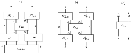
In this paper we provide a framework to certify nonlocal properties of quantum channels, in the presence of dephasing noise. To this end, we use measurement protocols depicted in Fig 1 to formulate (semi-)device independent criteria to certify nonlocality of quantum channels. This approach includes and extends existing methods [8, 17] and allows us to identify the role of dephasing noise in the nonlocal properties of quantum channels: while local dephasing cannot generate nonlocality, there are cases in which a global dephasing operation can generate both entanglement and nonlocality. Our analysis in the case of complete decoherence yields simple criteria to detect nonlocality in quantum channels through a geometric insight into the transition from quantum to classical operations.
II Preliminaries
II.1 Quantum and classical states and channels
The set of quantum states acting on a Hilbert space of dimension is represented by . The set of classical states, namely the -dimensional probability simplex, is denoted by . A classical channel transforming probability distributions is a stochastic matrix, that is, a matrix with non-negative entries that sum up to one in each column. The set of stochastic matrices with the dimension of inputs and outputs equal to is represented by . Analogously, completely positive (CP) and trace preserving (TP) maps, , also known as quantum operations or quantum channels, transform quantum states. Their inputs and outputs are density matrices acting on a Hilbert space and with dimensions and , respectively. When the input and output systems are held by the same party, we will denote by the joint system and use the notation , or simply , if no confusion arises.
We denote by (or simply ) the Choi matrix acting on , which defines a quantum channel through the Choi-Jamiołkowski isomorphism [28, 29],
| (1) |
The complete positivity and trace preserving (CPTP) conditions require that and
| (2) |
where we denote the partial trace by omitting the traced subsystems.
Following [30, 31], we denote a quantum superchannel as a bipartite channel with the special property that it transforms Choi matrices to Choi matrices. That is, a quantum channel is transformed according to
| (3) |
For the above to hold, the Choi matrix of should satisfy [31]
| (4a) | ||||
| (4b) | ||||
| (4c) | ||||
Similarly, a classical superchannel [32], transforming stochastic matrices of size to those of size , is isomorphic to a bipartite stochastic matrix of dimension . To be a valid superchannel, it has to additionally satisfy
| (5) |
The set of quantum and classical superchannels acting on -dimensional channels are respectively denoted by and .
II.2 Nonlocality of bipartite distributions
A bipartite probability distribution describes independent events when it is a product of local distributions, . The convex closure of these forms the Bell local distributions (L) [2, 14], decomposing as
| (6) |
where , . Otherwise, the distribution is called Bell nonlocal.
In quantum theory, probabilities are obtained through Born’s rule,
| (7) |
for some shared state and measurement effects and . Distributions obtained from Eq. (7) are called quantum (Q).
A probability distribution is called nonsignaling (NS) if it has well-defined marginals, i.e., it satisfies
| (8a) | ||||
| (8b) | ||||
The sets L, Q and NS are convex and form a chain of inclusions
| (9) |
Thus, they can be separated with linear functionals
| (10) |
on the space of bipartite probability distributions, called Bell functionals. One denotes the maximum value of a Bell functional over the set of distributions inside a selected subset (typically L, Q or NS). For example, the CHSH functional satisfies , and .
II.3 Nonlocality in quantum states
A Bell protocol is a device independent local measurement protocol where a bipartite probability distribution is obtained from a bipartite quantum state through Eq. (7). Assuming quantum theory, the only subsets of bipartite distributions that can be obtained in this way are local (L) or quantum (Q). Separable quantum states can only produce local correlations, and therefore observing nonlocal quantum correlations is an indicator of the presence of entanglement [33, 34]. A quantum state which cannot produce nonlocal correlations in the bipartition will be called a local state in such bipartition.
Remarkably, not all entangled states can produce correlations outside of L through Eq. (7), namely there exist local but entangled states [6, 35]. However, a subtle difference exists between separable and entangled states in certain measurement protocols: it was shown by Buscemi that all entangled states produce correlations that cannot be obtained from separable states in a semi-device independent protocol with trusted quantum inputs [15],
| (11) |
Here the inputs are fixed sets of quantum states and used in ancillary systems and . Distributions that cannot be obtained in this way from separable states are known as Buscemi nonlocal. For example, consider a state that is entangled but cannot produce distributions out of L through Eq. (7) [6]. Through Eq. (11), such a state produces distributions that are inside the local polytope L, but are Buscemi nonlocal and therefore denote entanglement. Quantum measurement protocols obtained through Eq. (11) are called Buscemi protocols to distinguish them from Bell protocols in Eq. (7).
II.4 Nonlocality of bipartite channels
Bipartite classical channels are characterized by bipartite stochastic matrices [36, 37, 38, 39], which are by definition isomorphic to bipartite correlations. That is to say, by arranging a conditional probability distribution in a matrix with columns labeled by , one obtains a bipartite stochastic matrix. This implies that the nonlocal structure of bipartite correlations defines accordingly a nonlocal structure in the set of bipartite stochastic maps. In particular, consider bipartite stochastic matrices of the form
| (12) |
where and are stochastic matrices. These stochastic matrices correspond with local probability distributions that decompose as Eq. (6), and thus we call them local stochastic matrices.
In the framework of quantum channel nonlocality, we distinguish the following three classes of channels.
-
•
Local operations assisted by shared randomness (LOSR): Operations which can be represented as the convex combination of local operations – tensor product of quantum channels,
(13) where , and are quantum channels. These are the free operations in the resource theory of both Bell and Buscemi nonlocality [40, 41, 17, 42] and are analogous to separable bipartite quantum states. Channels outside the set of LOSR are termed nonlocal and can be compared to entangled states.
- •
-
•
Causal, or quantum nonsignaling (qNS): Operations where Bob’s (Alice’s) output cannot be influenced by Alice’s (Bob’s) local operations [43, 45]. The marginals of their four-partite Choi matrices satisfy
(15a) (15b) Analogous to nonsignaling correlations in Eq. (8), nonsignaling channels have also well-defined marginal channels proportional to and .
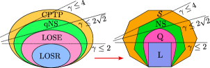
We have the chain of inclusions (see Fig. 2)
| (16) |
II.5 The effect of dephasing noise in quantum states and channels
Here we will consider quantum noise producing decoherence through a dephasing channel , which leaves invariant the occupations of the input state in a preferred basis , , while damping or inducing phases on the coherences. By imposing that a dephasing channel is a CPTP map, one verifies that it acts as [46, 47, 48, 49]
| (17) |
for some Gram matrix , i.e., a non-negative matrix with diagonal entries equal to one. Here denotes the Schur product (also called entry-wise or Hadamard product). That is, where .
Dephasing noise can lead to the full or partial loss of the resource of coherence [50], which plays a crucial role in most quantum protocols [51, 52, 53]. The reason why the definition of the dephasing noise is basis dependent, is because quantum protocols take place by measuring the inputs and outputs in a fixed basis which is determined by physical principles, e.g. the energy eigenbasis in Hamiltonian dynamics or the basis where measurements are performed in a given protocol [51, 52, 53, 54].
Similarly as for quantum states, the decoherent noise acting on a quantum channel through dephasing leaves invariant the diagonal entries of the Choi matrix in a preferred basis and damps the cross-terms [49]. A Choi matrix describing a channel is converted into where is a Gram matrix with some additional structure [49]. The most general form of such dephasing transformation is realized by pre- and post-processings along with memory [30]. Assuming that there is no memory, dephasing noise acts as where means concatenation. Then, the Choi matrix of a quantum channel is mapped to [49]
| (18) |
II.6 Complete decoherence: from quantum to classical
Consider now complete decoherence occurring by a completely dephasing channel , acting as in Eq. (17) where . Then, a quantum state loses all off-diagonal terms and becomes a probability vector . Similarly, when complete decoherence occurs in both the input and output systems of a quantum channel , the resulting operation is given by the diagonal of the Choi matrix [49]. That is, one has
| (19) |
where embeds a vector into the diagonal of a matrix. The CPTP condition on implies that the vector can be reshaped into a stochastic matrix , which is a linear map between the - and -dimensional probability simplices. The stochastic map , known as classical action [54, 55, 49, 56, 57], will be called here the decoherent action of [49] to emphasize that it corresponds to a possibly nonlocal channel arising from the effects of decoherence. The decoherent action can be obtained from Kraus operators of through , where * denotes the complex conjugation [58].
The effect of complete decoherence on quantum sets discussed above is summarized in Fig. 5. These sets are obtained from the set of four-partite states in different ways. Bipartite and monopartite states are obtained by partial trace. The probability simplices of corresponding sizes are obtained from these sets under decoherence. Bipartite and monopartite quantum channels are obtained from four-partite and bipartite states through the cross-section of Eq. (2). In particular, a generic quantum state with full-rank gives a generic quantum channel through where and imposes the partial trace condition [59]. Then a classical map (stochastic matrix) is obtained due to decoherence as in Eq. (19) from the diagonal entries of the Choi matrix describing the bipartite channel. The transition from channels to superchannels can be seen as an extended Choi-Jamiołkowski isomorphism, as superchannels are isomorphic to one-way quantum nonsignaling channels through Eq. (4c). These decohere to one-way nonsignalling distributions through Eq. (5).
Thus one identifies classical subsets embedded in quantum subsets at different levels: general distributions, conditional distributions and nonsignaling distributions are embedded in quantum states, channels and superchannels. In this way, recent studies on the geometry of the sets of local and nonlocal correlations [60, 22] are directly linked to the research on geometry of quantum states [58, 61] and geometry of quantum entanglement [62, 63]. Furthermore, analysis of the relative volume of the set of bipartite local correlations [64, 65, 66] can be compared with the problem of estimating the relative volume of the set of bipartite separable states [67, 68, 69, 70, 71].
III Channel nonlocality from local measurements
III.1 Local measurement protocols with shared entanglement
Bipartite distributions can be obtained from bipartite quantum channels by choosing input states and measuring their conditional outputs [8, 10, 16, 72], as shown in Fig. 1. In this spirit, consider the probability distribution obtained by the measurement protocol of Fig. 1 (a),
| (20) |
Proposition 1.
Let be a probability distribution obtained from a bipartite quantum channel through Eq. (20). For any input channels and and for any measurements and , the following holds:
-
(i)
If is in LOSR, then for any input state which is local in the bipartition , is in L.
-
(ii)
If is in LOSE, then for any shared state , is in Q.
-
(iii)
If is in qNS, then for any shared state , is in NS.
Proof.
Proof of (i). For any channel , we denote its adjoint by , which satisfies for any and . It is enough to consider an extremal LOSR operation , since the rest of the proof follows by convex combinations. Define the operators
| (21a) | ||||
| (21b) | ||||
Since the adjoint of a CPTP map is completely positive and unital, i.e., it satisfies [58], the operators () are positive semidefinite and their summation over () is the identity for any (). Thus, we can rewrite Eq. (20) as
| (22) |
which is a standard Bell game. Now it becomes evident by definition, that if the state is local in the bipartition , then a local distribution is obtained.
Proof of (ii). Consider an LOSE channel, which factorizes as in Eq. (14). Similarly as in the proof of item (i), define the measurement operators
| (23a) | ||||
| (23b) | ||||
Using Eqs. (23), one verifies that Eq. (20) reads
| (24) |
This proves that by applying an LOSE channel one can only recover quantum correlations.
Proof of (iii). By imposing in Eq. (20) that satisfies , we obtain
| (25) |
where , which does not depend on . Similarly, by imposing we obtain that does not depend on and therefore is a nonsignaling distribution. ∎
Note that Proposition 1 provides a criterion to detect quantum channels outside of the sets LOSR, LOSE and qNS which is fully device independent, in the sense that none of the quantum devices (the shared state , the input channels and , and the measurements and ) is trusted.
III.2 Local measurement protocols without entanglement
Consider the protocol in Fig. 1 (b),
| (26) |
which was introduced in [8]. This can be obtained from Eq. (20) by considering a product state , so that the channels and act as state preparation channels producing input states and . LOSR channels produce local probability distributions from Eq. (26), as shown in [8]. This result can be extended for other classes of channels.
Corollary 2.
Let be a probability distribution obtained from a bipartite quantum channel through Eq. (26). The following holds, for any choice of input states and measurements:
-
(i)
If is LOSR, then is in L.
-
(ii)
If is LOSE, then is in Q.
-
(iii)
If is qNS, then is in NS.
Proof.
Proof of (i). Probability distributions obtained from Eq. (26) with local operation factorize, thus LOSR channels give local probability distributions.
Proof of (ii). Similarly as in the proof of Prop. 1, define
| (27a) | ||||
| (27b) | ||||
One verifies that in Eq. (26) reads
| (28) |
Proof of (iii). This follows from Proposition 1. ∎
Two remarks are now in order. On the one hand, note that the converse of Corollary 2 is not true. In particular, channels denoted as local-limited in [8] always produce local correlations for any choice of input states and measurements. Examples are LOSE channels where Alice and Bob share an entangled state that cannot produce nonlocal correlations [6]. On the other hand, Eq. (28) implies that a bipartite LOSE channel produces nonlocal correlations if the shared state in Eq. (14) is nonlocal in some Bell protocol. This in turn dictates that if the shared state in one realization of an LOSE channel is Bell nonlocal, the channel cannot be realized by some shared local state.
III.3 A Buscemi-like characterization of LOSR operations
The results of Buscemi [15] extend to more general processes [17]. In particular, for a fixed channel and a fixed Bell functional , we denote as the maximal value of that can be achieved when the conditional probability distribution is obtained by a fixed set of input states and over all possible measurements and , i.e.,
| (29) |
where is obtained through Eq. (26).
The setup depicted in Fig. 1 (b) can be seen as a particular case of so-called semi-quantum games, which are known to characterize convertibility of general processes through free operations in a generalized theory of nonlocality [17]. In particular, the setup described in Eq. (26) and Fig. 1 (b) provides semi-quantum games characterizing local transformations between LOSR quantum channels. The following follows from [17, Corollary 1]:
Proposition 3.
Given two bipartite quantum operations and , can be transformed into by a convex combination of product superchannels if and only if for all Bell functionals and for all sets of input states, , where is given by Eq. (29).
The proof of the only if direction can be easily seen as follows. If can be converted into by a product of superchannels (or a convex combination of them), then we can absorb such product of superchannels in the state preparations and measurements of semiquantum games, described in Eq. (26) and depicted in Fig. 1 (b). Then it becomes clear that for all functionals . The proof for the if direction is based on the observation that Eq. (26) gives a distribution after local superchannels are performed in the form of , thus preserving the set of LOSR operations [17]. An explicit constructive proof is given in Appendix A.
Similarly as in [15], this means that a quantum channel is not LOSR if and only if it has a strictly larger value than any LOSR operation for some Bell functional and quantum inputs. The derivations in Appendix A provide explicit necessary and sufficient conditions to certify non-LOSR operations. Consider a set of fixed states and that are linearly independent and span the whole input spaces of linear operators acting on and , and assume and . Let and be projective measurements on a generalized Bell basis and denote
| (30) | ||||
This setup allows to formulate the problem of whether or not a channel is LOSR as follows: A quantum channel is not an LOSR operation if and only if for any possible LOSR operation and for any choice of measurements and , the distribution of Eq. (30) cannot be obtained via . By absorbing the adjoint in the measurements , namely defining , one arrives at the following criterion.
Corollary 4.
A bipartite quantum channel is not LOSR if and only for some functional
| (31) |
where we denote .
This provides a separation between the set of LOSR operations and the rest, which relies only in the input/outcome probabilities and the trusted set of input states and . Therefore, it constitutes a measurement-device independent characterization of the set of LOSR operations. Note that the left hand side of Eq. (31) is given by the set of input states and the channel under consideration, and the right hand side can be upper-bounded with semidefinite programming [73].
IV The role of dephasing noise
IV.1 Gradual dephasing
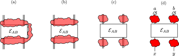
Quantum channels, and in particular the protocols described above to certify nonlocality, can suffer from decoherence. Here we ask how dephasing noise affects the nonlocal properties of a channel. Let us first consider local dephasing (Fig. 3 (c)), which is given by a local four partite Gram matrix of the form
| (32) |
Observation 5.
If a bipartite channel undergoing local dephasing noise, , can produce correlations outside of L (Q, NS) from Eq. (26), then the channel is not LOSR (LOSE, qNS).
Indeed, note that the Schur product with a Gram matrix preserves both positive semidefiniteness, the trace, and identity resolution of any operators. Therefore, local dephasing is absorbed in the preparation and measurement of any protocol. This means that if we detect nonlocality on a channel which suffered from local dephasing, then we know that its noiseless version previous to dephasing is also nonlocal.
Let us now consider the case in which the two parties and sharing a quantum state or implementing a quantum channel belong to a joint subsystem. In this case, dephasing can occur as a joint operation (Fig. 3 (a & b)), and thus one might expect that nonlocal phenomena can occur. This can be summarized as follows.
Proposition 6.
Dephasing noise acting jointly on a bipartite system has the following properties:
-
1.
A dephasing channel acting on a separable bipartite state can generate an entangled state.
-
2.
A dephasing superchannel acting on an LOSR operation can generate a nonlocal channel.
At the level of quantum states, an extreme example can be constructed as follows: Consider the states . Note that the projector has homogeneous entries , thus it evolves under dephasing noise in Eq. (19) given by some Gram matrix as
| (33) |
Therefore, it is enough to show that there exists a quantum state that is both maximally entangled and a Gram matrix. Indeed, the Bell state has density matrix
| (34) |
which defines a Gram matrix with entries where . Since is maximally entangled, it maximally violates Clauser-Horne-Shimony-Holt (CHSH) inequality,
| (35) |
where and are Pauli matrices and . From a resource theory perspective, this is possible because the state maximizes the resource of coherence (with respect to the computational basis) [74, 50], from which a dephasing channel can generate entanglement.
At the level of quantum channels, this example can be seen as follows: Consider the identity channel id, with the bipartite input state . Although the identity channel is an LOSR operation and thus produces probability distributions in local measurement protocols like the one of Eq. (26) (Fig 1), dephasing induced by coupling degrees of freedom with the environment can convert the channel id into a channel capable of generating nonlocal quantum probability distributions. This is an example where dephasing occurs as a superchannel with independent pre- and post-processing [49, 30] (Fig. 3 (b)).
An example where dephasing is induced by a more general superchannel (Fig. 3 (a)) is as follows: Consider the Choi matrix of the local unitary . Let the dephasing superchannel be described by a Gram matrix with nonzero coefficients , , and (and their Hermitian adjoints), where is the imaginary unit. This dephasing leads to the Choi matrix which defines the channel implementing the following unitary,
| (36) |
Observe that this unitary can be converted into the C-NOT gate by local unitaries as follows,
| (37) |
and therefore can produce extremal signaling probability distributions in the protocol in Fig. 1 (b) when decoherence depicted in Fig. 3 (a) occurs.
Let us highlight that the examples above constitute a special case of dephasing channels and superchannels occurring to highly coherent states and channels, whose coherence only suffer from phase factors. Although these examples are consistent with the mathematical model of dephasing operations established in [49], generic dephasing transforms pure states into mixed states, and unitary channels into irreversible channels [20]. Yet, these examples are illustrative for the following comparison: Observation 5 captures the intuitive fact that decohrence might make a nonlocal quantum channel undetectable through measurement protocols, thus giving a false negative result to a test of nonlocality. On the contrary, Propopsition 6 shows that decoherence can also give rise to false positive results if the parties and perform a measurement protocol undergoing nonlocal noise.
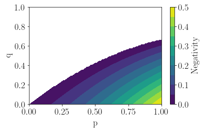
To better understand the role of gradual decoherence aside from extremal cases, we consider two parametric types of dephasing models. On one hand, damps all off-diagonal terms equally, . On the other hand, keeps all entries except for the coherences to the fourth population level, namely if either or .
Starting from the maximally coherent separable state , the composition of these two noises reads
| (38) |
with . The negativity of this state for the parameters and is shown in Fig. 4.
IV.2 Complete decoherence
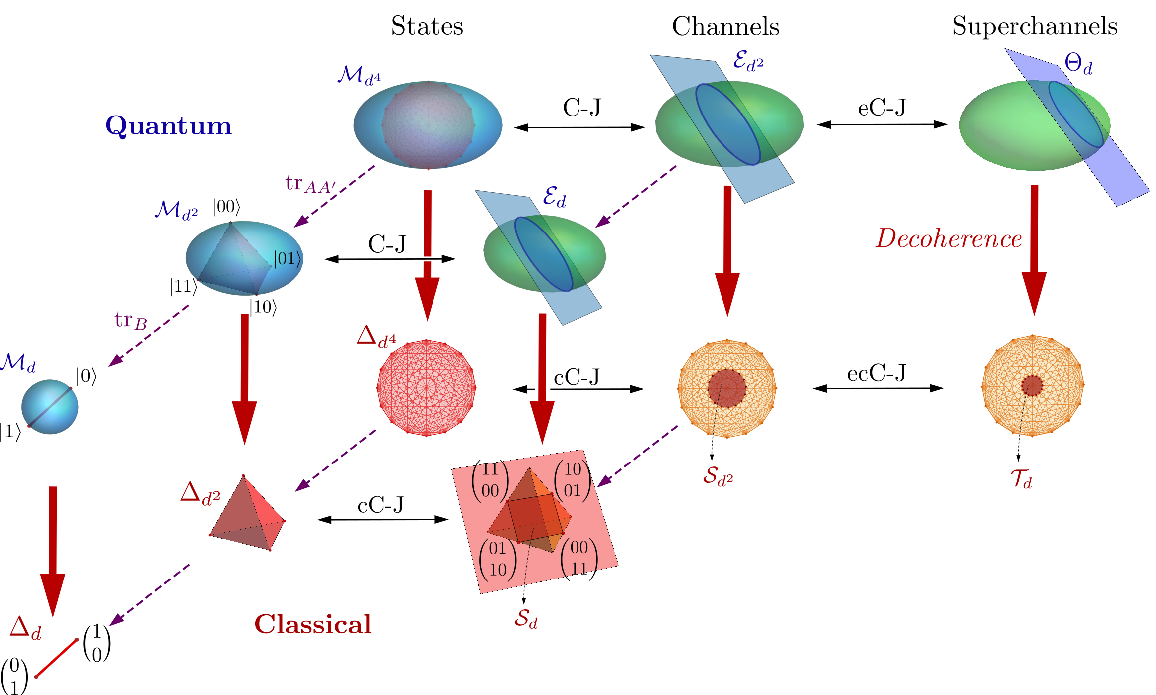
Here we consider the case of complete decoherence depicted in Fig. 5, where Choi matrices become diagonal. Recall that the set of stochastic matrices and the set of conditional probability distributions are isomorphic. For bipartite channels , the decoherent action is represented by a bipartite stochastic matrix with entries
| (39) |
where define the canonical basis (Fig. 5). Therefore, the decoherent action (39) defines probabilities of obtaining classical outputs conditioned to classical inputs , through the scheme of Fig. 1 (c). In [8, Propositions 3-5] it was shown that the sets of L, Q and NS correlations correspond to the sets of correlations that can be obtained respectively from LOSR, LOSE, and qNS channels as correlations in the inputs and outputs when all measurement bases are allowed. A similar result can be formulated for a fixed basis, namely considering the decoherent action of Eq. (39), as follows.
Proposition 7.
The following equivalences hold:
-
(i)
The set of local (L) correlations coincides with the set of decoherent actions of LOSR channels.
-
(ii)
The set of quantum (Q) correlations coincides with the set of decoherent actions of LOSE channels.
-
(iii)
The set of nonsignaling (NS) correlations coincides with the set of decoherent actions of quantum nonsignaling channels qNS.
Proposition 7 can be obtained from [8, Prop. 3, 4 & 5], by absorbing the basis choice into the existence conditions. An explicit constructive proof is given in Appendix B. This provides a simple criterion to detect certain classes of quantum channels, from local measurements in the computational basis: One certifies that a quantum channel is outside of the set of LOSR (LOSE, qNS) channels if its decoherent action is outside of the set of L (Q, NS) correlations. This criterion can be implemented in decoherent setups, as it involves only measurements in the computational basis.
Let us highlight that the converse is not true: there exist non-LOSR quantum channels with local decoherent action. As an example, consider the 2-qubit channel with unitary (single) Kraus operator , which maps the computational basis to the Bell states where and are Pauli matrices. Even though can generate entanglement, its decoherent action is local. However, note that this criterion can be enhanced with any operations that preserve the set of LOSR. In the example above, the freedom of local measurement basis considered in [8] is enough: the bipartite unitary can be transformed by local unitaries to , where is the Hadamard gate with and . We have which defines extremal nonsignaling correlations.
Note that the nonsignaling conditions establish equality constraints, and thus define a measure zero subset of channels. Moreover, the sets of local and nonsignaling correlations form a polytope. Therefore, detecting channels with nonlocal decoherent action can be done with a linear program, asking whether there exists a convex combination of extremal local stochastic matrices decomposing the decoherent action. For local correlations, finitely-many Bell games [75, 76, 14] equivalently define the faces of their polytope. Bounding the set of quantum correlations is a more involved problem and relies on a convergent hierarchy [77]. This problem has been tackled through analytical solutions for the smallest setting [78, 79, 80], conjectured generalizations [60, 81] and additional results using semidefinite programming techniques [82, 83]. Outer approximations are given by the maximum quantum value of Bell games [84].
By Proposition 7, Bell functionals on the decoherent action of a quantum channel can be used to construct linear nonlocality witnesses, similar to entanglement witnesses [34]. This mechanism is illustrated in Fig. 2. Let be one of the three subsets of bipartite quantum channels: LOSR, LOSE, and qNS. Let be the corresponding set of bipartite probability distributions under the correspondence in Prop. 7, namely, L, Q, and NS. Consider
| (40) |
where is defined from the Bell functional through
| (41) |
and denotes its maximum value on the subset . Thus, a channel with Choi matrix and decoherent action is outside if
| (42) |
For the CHSH functional, , it holds that , and .
On the other hand, by the isomorphism of Proposition 7, any bipartite stochastic matrix in a distinguished subset of correlations can be obtained from decoherence of a quantum channel in a corresponding subset. An explicit example is the convex hull of bipartite stochastic matrices (namely, bipartite probability distributions) with
| (43) |
which attains the maximal quantum value of CHSH for .
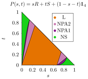
In Fig. 6 we show a two dimensional slice of the polytope of distributions consisting of the convex hull of , and containing different subsets. The sets of local (L) and nonsignaling (NS) distributions are bounded by linear programming, while the set of quantum (Q) distributions is approximated by the first two levels of the Navascués-Pironio-Acín (NPA) hierarchy [77]. The subsets L, Q and NS of distributions are obtained by decoherence of the subsets LOSR, LOSE and qNS of channels.
V Conclusions and open questions
We infer nonlocal properties of bipartite quantum channels based on the bipartite stochastic matrices produced by them under measurement protocols. In particular, our approach allows us to bound the sets of local operations assisted by shared randomness (LOSR), local operations assisted by shared entanglement (LOSE) and quantum non-signaling channels (qNS), from the conditional probabilities of local measurement outcomes. This framework is suitable to experimental verification of nonlocality of bipartite channels from local measurements, even in the presence of complete decoherence. In contrast, we show that both entanglement and nonlocality of bipartite quantum channels can be enhanced under nonlocal gradual decoherence.
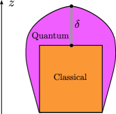
This work relates the geometry of the set of bipartite quantum states, channels, superchannels, and their classical counterparts: probability vectors, stochastic matrices and classical superchannels. In particular, several measures for nonlocality in the space of correlations have been proposed in the literature [85, 86, 87, 64]. Through our framework, these naturally give insight into the geometry of quantum operations [67]. At the same time, our work leaves several research lines open:
- 1.
-
2.
Corollary 4 provides a first step to understanding the set of functionals witnessing non-LOSR operations, analogous to entanglement witnesses for nonseparable states. However, further research is needed to better understand the performance of such witnesses in practice.
The analysis presented for the case of complete decoherence highlights the role of Choi–Jamiołkowski isomorphism to analyze geometric features of quantum correlations and channel nonlocality. The standard form of the isomorphism relates bipartite states with quantum operations, while its generalized version links four-partite quantum states with bipartite quantum channels. Due to decoherence the latter suffer a transition to bipartite stochastic matrices , which describe correlations between both systems. Therefore, the overall geometric structure of the sets of classical and quantum states, channels and correlations is rooted in the geometric structure of the set four-partite states (Fig. 5).
Any generalized quantum theory can be recovered from basic principles that force the corresponding set of states to be convex [88]. Hence, if one looks into the set of density matrices from a large perspective, one realizes that it forms a convex set [89]. A closer look reveals its convex subset of separable states, defined as classical mixtures of product states – see Fig. 7. A related structure is characteristic also to the space of quantum maps and quantum correlations. A similar picture can also be used to describe the sets of quantum algorithms and quantum technologies and to visualize the notion of a quantum advantage: The difference between the utility function describing, for instance, efficiency of a given protocol, optimized over all quantum and classical scenarios.
Acknowledgements: We are thankful to Remigiusz Augusiak, Francesco Buscemi, Dariusz Chruściński, Felix Huber, Kamil Korzekwa, Miguel Navascués, Roberto Salazar, Anna Sanpera and Mario Ziman for discussions and for pointing to references. Support by the Foundation for Polish Science through TEAM-NET project POIR.04.04.00-00-17C1/18-00 and by NCN QuantERA Project No. 2021/03/Y/ST2/00193 is gratefully acknowledged. FS acknowledges projects DESCOM VEGA 2/0183/2 and DeQHOST APVV-22-0570.
Appendix A Proof of Proposition 3
Here we will prove the if part of Proposition 3. Namely, we will show that if is more nonlocal than for all the games specified in Fig. 1 (b), then it can be transformed to through some superchannels .
Proof.
We will follow a similar reasoning to the analogous result of Buscemi for bipartite quantum states [15]. To this end, consider the extended Hilbert spaces
| (44) | ||||
| (45) |
Note that the input and output dimensions of the channels and in consideration can in general be different. Therefore, the subsystems , and (, , and ) shall be chosen accordingly such that the dimensions match. In particular, we set the dimension () to be a common multiple of the input dimensions and ( and ). Namely, there exist natural numbers , , and so that
| (46) | ||||
| (47) |
Thus, the input states and are regarded in different bipartitions when they are used as input states for the different channels and . For example, suppose we consider a channel with and a channel with . Then we can consider an input state , which can be seen either as a bipartite state with and , or as a bipartite state with and .
In a similar manner, consider the convex combinations of local measurements in the output systems and , . Following the same arguments in the proof of Proposition 1 of [15], notice that the probability distributions available for a particular game with different measurements form a convex set. Therefore, for all is equivalent to assuming for any measurement of the above form there exists a measurement in the convex hull of local measurements such that
| (48) |
Define now the input states as
| (49a) | ||||
| (49b) | ||||
with extended Hilbert spaces and , where and are informationally complete, positive operator-valued measurements (IC-POVMs) and is the density matrix of the Bell state (and similarly for ). For convenience we will denote and . Thus, we can write Eq. (48) as
| (50) |
Now divide the full trace above as . By assumption, and are IC-POVMs and therefore form a basis for the linear operators acting on the Hilbert spaces and . As a result, for the partial trace over and , we have the following
| (51) |
Let us now recover the notation and while noticing that , and the same for . Thus, we can write
| (52) | |||
On each side of the equality, we identify the Choi states and tensored by two pairs of Bell states . This allows for a physical interpretation in terms of teleportation similar to [15], with the difference that now two parts out of the four-partite Choi state are teleported. That is, here Alice holds the systems , , and and Bob holds the systems , , and . Using two shared Bell states, and , Alice teleports her parts and of the shared Choi state to Bob’s parts and .
By assumption, for any there exists a such that the equality Eq. (52) holds. In particular, it holds when Alice applies a Bell measurement to send her side to Bob, where is the density matrix of each generalized Bell state [51]. In this case, Bob can apply unitaries to recover in his side. Strictly speaking,
| (53) | ||||
where we inserted the left-hand side of Eq. (52) as the (unnormalized) state Bob obtains for each outcome and of Alice. Finally, expanding with and , one gets the following maps
| (54) | ||||
| (55) |
One can verify that if , thus each is a quantum superchannel. Similarly, each is a superchannel. It is now clear that the Choi matrix can be obtained through local operations assisted by shared randomness from ,
| (56) |
which means that the channel can be obtained from the channel by a convex combination of products of superchannels. ∎
Appendix B Proof of Proposition 7
Let us show first item (ii). Let determine a quantum probability distribution, where is a quantum state on , projective measurements over and over . Going to a Stinespring’s dilation, there exist unitary maps and such that
| (57) |
Take and unitaries on some control systems and ,
| (58) |
These define a LOSE channel via
| (59) |
whose decoherent action gives back . Indeed,
| (60) |
thus reads
| (61) |
Conversely, assume can be obtained as the decoherent action of a LOSE channel, , where and are unitaries and a state on . With the isometries
| (62) |
we can define quantum effects
| (63) |
that reproduce the probabilities . Indeed,
| (64) |
Item (i) follows from the above derivations by considering to be a separable state. Item (iii) can be seen by realizing that the qNS conditions on a diagonal Choi matrix are equivalent to the NS conditions on the probability distribution given by the decoherent action of the channel.
References
- Bell [1964] J. S. Bell, On the Einstein Podolsky Rosen paradox, Phys. Phys. Fiz. 1, 195 (1964).
- Bell [1966] J. S. Bell, On the problem of hidden variables in quantum mechanics, Rev. Modern Phys. 38, 447 (1966).
- Wiesner [1983] S. Wiesner, Conjugate coding, ACM SIGACT News 15, 78 (1983).
- Pironio et al. [2010] S. Pironio, A. Acín, S. Massar, A. B. de La Giroday, D. N. Matsukevich, P. Maunz, S. Olmschenk, D. Hayes, L. Luo, T. A. Manning, and C. Monroe, Random numbers certified by Bell’s theorem, Nature 464, 1021 (2010).
- Bennett and Brassard [1984] C. H. Bennett and G. Brassard, Quantum cryptography: Public key distribution and coin tossing, Theoret. Comput. Sci. 560, 7 (1984).
- Werner [1989] R. F. Werner, Quantum states with Einstein-Podolsky-Rosen correlations admitting a hidden-variable model, Phys. Rev. A 40, 4277 (1989).
- Barrett [2002] J. Barrett, Nonsequential positive-operator-valued measurements on entangled mixed states do not always violate a Bell inequality, Phys. Rev. A 65, 042302 (2002).
- Hoban and Sainz [2018] M. J. Hoban and A. B. Sainz, A channel-based framework for steering, non-locality and beyond, New J. Phys. 20, 053048 (2018).
- Rosset et al. [2018] D. Rosset, F. Buscemi, and Y.-C. Liang, Resource theory of quantum memories and their faithful verification with minimal assumptions, Phys. Rev. X 8, 021033 (2018).
- Selby et al. [2023] J. H. Selby, A. B. Sainz, V. Magron, Ł. Czekaj, and M. Horodecki, Correlations constrained by composite measurements, Quantum 7, 1080 (2023).
- Massar et al. [2002] S. Massar, S. Pironio, J. Roland, and B. Gisin, Bell inequalities resistant to detector inefficiency, Phys. Rev. A 66, 052112 (2002).
- Acín et al. [2002] A. Acín, T. Durt, N. Gisin, and J. I. Latorre, Quantum nonlocality in two three-level systems, Phys. Rev. A 65, 052325 (2002).
- Brito et al. [2018] S. G. A. Brito, B. Amaral, and R. Chaves, Quantifying Bell nonlocality with the trace distance, Phys. Rev. A 97, 022111 (2018).
- Brunner et al. [2014] N. Brunner, D. Cavalcanti, S. Pironio, V. Scarani, and S. Wehner, Bell nonlocality, Rev. Mod. Phys. 86, 419 (2014).
- Buscemi [2012] F. Buscemi, All entangled quantum states are nonlocal, Phys. Rev. Lett. 108, 200401 (2012).
- Zjawin et al. [2023a] B. Zjawin, D. Schmid, M. J. Hoban, and A. B. Sainz, The resource theory of nonclassicality of channel assemblages, Quantum 7, 1134 (2023a).
- Schmid et al. [2020] D. Schmid, D. Rosset, and F. Buscemi, The type-independent resource theory of local operations and shared randomness, Quantum 4, 262 (2020).
- Liu and Yuan [2020] Y. Liu and X. Yuan, Operational resource theory of quantum channels, Phys. Rev. Res. 2, 012035 (2020).
- Peres [1998] A. Peres, Quantum Theory: Concepts and Methods, Vol. 72 (Kluver Academic, London, 1998).
- Nielsen and Chuang [2010] M. A. Nielsen and I. L. Chuang, Quantum Computation and Quantum Information: 10th Anniversary Edition (Cambridge University Press, 2010).
- Schlosshauer [2007] M. Schlosshauer, Decoherence and the Quantum-to-Classical Transition (Springer, The Frontiers Collection, 2007).
- Rahman et al. [2022] A. U. Rahman, Y. Khedif, M. Javed, H. Ali, and M. Daoud, Characterizing two-qubit non-classical correlations and non-locality in mixed local dephasing noisy channels, Ann. Phys. 534, 2200197 (2022).
- Breuer and Petruccione [2007] H.-P. Breuer and F. Petruccione, The Theory of Open Quantum Systems (Oxford University Press, 2007).
- Wiseman and Milburn [2009] H. M. Wiseman and G. J. Milburn, Quantum measurement and control (Cambridge university press, 2009).
- Devetak and Shor [2005] I. Devetak and P. W. Shor, The capacity of a quantum channel for simultaneous transmission of classical and quantum information, Commun. Math. Phys. 256, 287 (2005).
- D’Arrigo et al. [2007] A. D’Arrigo, G. Benenti, and G. Falci, Quantum capacity of dephasing channels with memory, New J. Phys. 9, 310 (2007).
- Brádler et al. [2010] K. Brádler, P. Hayden, D. Touchette, and M. M. Wilde, Trade-off capacities of the quantum hadamard channels, Phys. Rev. A 81, 062312 (2010).
- Choi [1975] M.-D. Choi, Completely positive linear maps on complex matrices, Linear Algebra Appl. 10, 285 (1975).
- Jamiołkowski [1972] A. Jamiołkowski, Linear transformations which preserve trace and positive semidefiniteness of operators, Rep. Math. Phys. 3, 275 (1972).
- Chiribella et al. [2008] G. Chiribella, G. M. D’Ariano, and P. Perinotti, Transforming quantum operations: Quantum supermaps, Europhys. Lett. 83, 30004 (2008).
- Gour [2019] G. Gour, Comparison of quantum channels by superchannels, IEEE Trans. Inf. Theory 65, 5880 (2019).
- Hasenöhrl and Caro [2022] M. Hasenöhrl and M. C. Caro, Quantum and classical dynamical semigroups of superchannels and semicausal channels, J. Math. Phys. 63, 072204 (2022).
- Hyllus et al. [2005] P. Hyllus, O. Gühne, D. Bruß, and M. Lewenstein, Relations between entanglement witnesses and Bell inequalities, Phys. Rev. A 72, 012321 (2005).
- Gühne and Tóth [2009] O. Gühne and G. Tóth, Entanglement detection, Phys. Rep. 474, 1 (2009).
- Vértesi and Brunner [2014] T. Vértesi and N. Brunner, Disproving the Peres conjecture by showing Bell nonlocality from bound entanglement, Nat. Commun. 5, 5297 (2014).
- Jones and Masanes [2005] N. S. Jones and L. Masanes, Interconversion of nonlocal correlations, Phys. Rev. A 72, 052312 (2005).
- Barrett [2007] J. Barrett, Information processing in generalized probabilistic theories, Phys. Rev. A 75, 032304 (2007).
- Gallego et al. [2012] R. Gallego, L. E. Würflinger, A. Acín, and M. Navascués, Operational framework for nonlocality, Phys. Rev. Lett. 109, 070401 (2012).
- de Vicente [2014a] J. I. de Vicente, On nonlocality as a resource theory and nonlocality measures, J. Phys. A 47, 424017 (2014a).
- Geller and Piani [2014] J. Geller and M. Piani, Quantifying non-classical and beyond-quantum correlations in the unified operator formalism, J. Phys. A 47, 424030 (2014).
- de Vicente [2014b] J. I. de Vicente, On nonlocality as a resource theory and nonlocality measures, J. Phys. A 47, 424017 (2014b).
- Rosset et al. [2020] D. Rosset, D. Schmid, and F. Buscemi, Type-independent characterization of spacelike separated resources, Phys. Rev. Lett. 125, 210402 (2020).
- Beckman et al. [2001] D. Beckman, D. Gottesman, M. A. Nielsen, and J. Preskill, Causal and localizable quantum operations, Phys. Rev. A 64, 052309 (2001).
- Schmid et al. [2021] D. Schmid, H. Du, M. Mudassar, G. Coulter-de Wit, D. Rosset, and M. J. Hoban, Postquantum common-cause channels: the resource theory of local operations and shared entanglement, Quantum 5, 419 (2021).
- Leung and Matthews [2015] D. Leung and W. Matthews, On the power of PPT-preserving and non-signalling codes, IEEE Trans. Inf. Theory 61, 4486 (2015).
- Kye [1995] S.-H. Kye, Positive linear maps between matrix algebras which fix diagonals, Linear Algebra Appl. 216, 239 (1995).
- Li and Woerdeman [1997] C.-K. Li and H. J. Woerdeman, Special classes of positive and completely positive maps, Linear Algebra Appl. 255, 247 (1997).
- Levick et al. [2017] J. Levick, D. W. Kribs, and R. Pereira, Quantum privacy and schur product channels, Rep. Math. Phys. 80, 333 (2017).
- Puchala et al. [2021] Z. Puchala, K. Korzekwa, R. Salazar, P. Horodecki, and K. Życzkowski, Dephasing superchannels, Phys. Rev. A 104, 052611 (2021).
- Winter and Yang [2016] A. Winter and D. Yang, Operational resource theory of coherence, Phys. Rev. Lett. 116, 120404 (2016).
- Bennett et al. [1993] C. H. Bennett, G. Brassard, C. Crépeau, R. Jozsa, A. Peres, and W. K. Wootters, Teleporting an unknown quantum state via dual classical and Einstein-Podolsky-Rosen channels, Phys. Rev. Lett. 70, 1895 (1993).
- Pan et al. [1998] J.-W. Pan, D. Bouwmeester, H. Weinfurter, and A. Zeilinger, Experimental entanglement swapping: Entangling photons that never interacted, Phys. Rev. Lett. 80, 3891 (1998).
- Bennett et al. [1988] C. H. Bennett, G. Brassard, and J.-M. Robert, Privacy amplification by public discussion, SIAM J. Comput. 17, 210 (1988).
- Korzekwa et al. [2018] K. Korzekwa, S. Czachórski, Z. Puchala, and K. Życzkowski, Coherifying quantum channels, New J. Phys. 20, 043028 (2018).
- Shahbeigi et al. [2021] F. Shahbeigi, D. Amaro-Alcalá, Z. Puchała, and K. Życzkowski, Log-convex set of Lindblad semigroups acting on N-level system, J. Math. Phys. 62, 072105 (2021).
- Korzekwa and Lostaglio [2021] K. Korzekwa and M. Lostaglio, Quantum advantage in simulating stochastic processes, Phys. Rev. X 11, 021019 (2021).
- Shahbeigi et al. [2023] F. Shahbeigi, C. T. Chubb, R. Kukulski, Ł. Pawela, and K. Korzekwa, Quantum-embeddable stochastic matrices (2023), arXiv:2305.17163 .
- Bengtsson and Życzkowski [2006] I. Bengtsson and K. Życzkowski, Geometry of Quantum States: an Introduction to Quantum Entanglement (Cambridge University Press, 2006).
- Kukulski et al. [2021] R. Kukulski, I. Nechita, Ł. Pawela, Z. Puchała, and K. Życzkowski, Generating random quantum channels, J. Math. Phys. 62, 062201 (2021).
- Goh et al. [2018] K. T. Goh, J. Kaniewski, E. Wolfe, T. Vértesi, X. Wu, Y. Cai, Y.-C. Liang, and V. Scarani, Geometry of the set of quantum correlations, Phys. Rev. A 97, 022104 (2018).
- Bengtsson et al. [2012] I. Bengtsson, S. Weis, and K. Życzkowski, Geometry of the set of mixed quantum states: An apophatic approach, in Geometric Methods in Physics (Springer Basel, 2012) p. 175–197.
- Kuś and Życzkowski [2001] M. Kuś and K. Życzkowski, Geometry of entangled states, Phys. Rev. A 63, 032307 (2001).
- Puchała et al. [2012] Z. Puchała, J. A. Miszczak, P. Gawron, C. F. Dunkl, J. A. Holbrook, and K. Życzkowski, Restricted numerical shadow and the geometry of quantum entanglement, J. Phys. A 45, 415309 (2012).
- Cabello [2005] A. Cabello, How much larger quantum correlations are than classical ones, Phys. Rev. A 72, 012113 (2005).
- Wolfe and Yelin [2012] E. Wolfe and S. F. Yelin, Quantum bounds for inequalities involving marginal expectation values, Phys. Rev. A 86, 012123 (2012).
- Duarte et al. [2018] C. Duarte, S. Brito, B. Amaral, and R. Chaves, Concentration phenomena in the geometry of Bell correlations, Phys. Rev. A 98, 062114 (2018).
- Życzkowski et al. [1998] K. Życzkowski, P. Horodecki, A. Sanpera, and M. Lewenstein, Volume of the set of separable states, Phys. Rev. A 58, 883 (1998).
- Slater [1999] P. B. Slater, A priori probabilities of separable quantum states, J. Phys. A 32, 5261–5275 (1999).
- Milz and Strunz [2014] S. Milz and W. T. Strunz, Volumes of conditioned bipartite state spaces, J. Phys. A 48, 035306 (2014).
- Lovas and Andai [2017] A. Lovas and A. Andai, Invariance of separability probability over reduced states in 4 × 4 bipartite systems, J. Phys. A 50, 295303 (2017).
- Sauer et al. [2021] A. Sauer, J. Z. Bernád, H. J. Moreno, and G. Alber, Entanglement in bipartite quantum systems: Euclidean volume ratios and detectability by Bell inequalities, J. Phys. A 54, 495302 (2021).
- Zjawin et al. [2023b] B. Zjawin, D. Schmid, M. J. Hoban, and A. B. Sainz, Quantifying EPR: the resource theory of nonclassicality of common-cause assemblages, Quantum 7, 926 (2023b).
- Berta et al. [2022] M. Berta, F. Borderi, O. Fawzi, and V. B. Scholz, Semidefinite programming hierarchies for constrained bilinear optimization, Math. Program. 194, 781–829 (2022).
- Baumgratz et al. [2014] T. Baumgratz, M. Cramer, and M. B. Plenio, Quantifying coherence, Phys. Rev. Lett. 113, 140401 (2014).
- Fine [1982] A. Fine, Hidden variables, joint probability, and the Bell inequalities, Phys. Rev. Lett. 48, 291 (1982).
- Rosset et al. [2014] D. Rosset, J.-D. Bancal, and N. Gisin, Classifying 50 years of Bell inequalities, J. Phys. A 47, 424022 (2014).
- Navascués et al. [2008] M. Navascués, S. Pironio, and A. Acín, A convergent hierarchy of semidefinite programs characterizing the set of quantum correlations, New J. Phys. 10, 073013 (2008).
- Tsirel’son [1987] B. S. Tsirel’son, Quantum analogues of the Bell inequalities. the case of two spatially separated domains, J. Sov. Math. 36, 557 (1987).
- Landau [1988] L. J. Landau, Empirical two-point correlation functions, Found. Phys. 18, 449 (1988).
- Masanes [2005] L. Masanes, Extremal quantum correlations for n parties with two dichotomic observables per site (2005), arXiv:quant-ph/0512100 .
- Mikos-Nuszkiewicz and Kaniewski [2023] A. Mikos-Nuszkiewicz and J. Kaniewski, Extremal points of the quantum set in the CHSH scenario: conjectured analytical solution (2023), arXiv:2302.10658 .
- Thinh et al. [2019] L. P. Thinh, A. Varvitsiotis, and Y. Cai, Geometric structure of quantum correlators via semidefinite programming, Phys. Rev. A 99, 052108 (2019).
- Le et al. [2023] T. P. Le, C. Meroni, B. Sturmfels, R. F. Werner, and T. Ziegler, Quantum correlations in the minimal scenario, Quantum 7, 947 (2023).
- Cirel’son [1980] B. S. Cirel’son, Quantum generalizations of Bell’s inequality, Lett. Math. Phys. 4, 93 (1980).
- Pironio [2003] S. Pironio, Violations of Bell inequalities as lower bounds on the communication cost of nonlocal correlations, Phys. Rev. A 68, 062102 (2003).
- Van Dam et al. [2005] W. Van Dam, R. D. Gill, and P. D. Grunwald, The statistical strength of nonlocality proofs, IEEE Trans. Inf. Theory 51, 2812 (2005).
- Barrett et al. [2005] J. Barrett, N. Linden, S. Massar, S. Pironio, S. Popescu, and D. Roberts, Nonlocal correlations as an information-theoretic resource, Phys. Rev. A 71, 022101 (2005).
- Mielnik [1974] B. Mielnik, Generalized quantum mechanics, Commun. Math. Phys. 37, 221 (1974).
- Mielnik [1980] B. Mielnik, Quantum Theory Without Axioms. Quantum Gravity II. A Second Oxford Symposium (1980).
