Structure-inspired Ansatz and Warm Start of Variational Quantum Algorithms for Quadratic Unconstrained Binary Optimization Problems

Abstract

This paper introduces a structure-inspired ansatz for addressing quadratic unconstrained binary optimization problems with the Variational Quantum Eigensolver. We propose a novel warm start technique that is based on imaginary time evolution, and allows for determining a set of initial parameters prioritizing lower energy states in a resource-efficient way. Using classical simulations, we demonstrate that this warm start method significantly improves the success rate and reduces the number of iterations required for the convergence of Variational Quantum Eigensolver. The numerical results also indicate that the warm start approach effectively mitigates statistical errors arising from a finite number of measurements, and to a certain extent alleviates the effect of barren plateaus.

I Introduction

The Variational Quantum Eigensolver (VQE) is a classical-quantum hybrid algorithm which relies on suitable circuit ansätze Peruzzo et al. (2014); Cerezo et al. (2021). Therefore, such approaches do not require deep quantum circuits which makes them suitable for noisy intermediate-scale quantum (NISQ) devices. VQE can be applied to many different scenarios, such as eigenvalue problems from physics and chemistry Meglio et al. (2023); Tilly et al. (2022), as well as to combinatorial optimization problems Chai et al. (2023a, b); Schwägerl et al. (2023); Amaro et al. (2022); Nannicini (2019). However, in order to be employed in practically useful applications, VQE needs to overcome a number of significant challenges, for example, the statical error due to the finite shots Scriva et al. (2024) and the presence of the barren plateaus McClean et al. (2018). These problems can prevent the optimization of VQE from converging to the global minimal efficiently. Thus, the choice of an appropriate ansatz and initial parameters for VQE is a way to help the optimization process. In this work, we investigate the quadratic unconstrained binary optimization (QUBO) problem to evaluate a structure-inspired ansatz (SIA), and develop a novel warm start approach corresponding to this ansatz. This approach leverages concepts from imaginary time evolution to emphasize lower energy states at initialization, potentially offering a more effective starting point than the typical universal superposition or random states. Our numerical simulation results indicate that VQE with the warm start is able to result in a higher success rate in finding the optimal solution with fewer iterations. Besides, the warm start shows a potential to mitigate the problems of statistical error and the barren plateaus.

The paper is organized as follows. Section II outlines the QUBO problem and the simulation setup. Subsequently, the structure-inspired ansatz inspired by imaginary time evolution is introduced in Sec. III. Moreover, its performance compared to a generic hardware-efficient ansatz (HEA) is assessed. Finally, we introduce a novel warm start approach in Sec. IV, as well as low-cost simplification thereof in Sec.V, which allows for determining the initial set of parameters classically. The improvement in performance of these methods is demonstrated using numerical simulation. Section VI shows the potential of the warm start to mitigate statistical errors and to alleviate the effect of barren plateaus. Finally, Sec. VII concludes with a summary and prospects for future research.

II QUBO and CVaR-VQE

In this paper we focus on the CVaR-VQE, a variant of the VQE proposed for combinatorial optimization problems Barkoutsos et al. (2020), and apply it to QUBO problems, both of which we review below. The QUBO problem is defined by a vector of $N$ binary variables $\mathbb{x}=\{x_{0},x_{i},\cdots x_{N-1}\}$ and the symmetric coefficient matrix $Q\in\mathbb{R}^{N\times N}$ as well as a cost function Kochenberger et al. (2014)

$$f(\mathbb{x})=\mathbb{x}^{T}Q\mathbb{x}=\sum_{i=0}^{N-1}\sum_{j=0}^{N-1}x_{i}\cdot Q_{ij}\cdot x_{j}.$$ (1)

The objective is to find the assignment of binary variables which minimizes the cost function for a given $Q$. A wide range of combinatorial optimization problems can be expressed in this mathematical framework, among them the optimal flight to gate assignment at an airport, particle tracking, job scheduling, and many others Chai et al. (2023a, b); Schwägerl et al. (2023); Amaro et al. (2022). Every QUBO problem can be associated with a graph by interpreting the matrix $Q$ as the adjacency matrix of a weighted, undirected graph $G(V,E)$. $V$ corresponds the set of vertices of size $|V|=N$, and $E$ represents the set of edges between vertex pairs $(i,j)$ for which $Q_{ij}=Q_{ji}\neq 0$.

QUBO problems can be straightforwardly represented as (quantum) Hamiltonians on $N$ qubits which are polynomials of Pauli-$Z$ operators Hadfield (2021). In particular, the corresponding Hamiltonian for $f(\mathbb{x})$ can be obtained by substituting the binary variables $x_{i}$ with the operator $\left(\mathds{1}-\sigma^{z}_{i}\right)/2$, where $\mathds{1}$ denotes the identity operator and $\sigma^{z}_{i}$ represents the Pauli-$Z$ operator acting on the $i$-th qubit. Using this substitution one finds for the Hamiltonian up to a constant

$$H=\sum_{i\in V}h_{i}\cdot\sigma^{z}_{i}+\sum_{(i,j)\in E}J_{ij}\cdot\sigma^{z}_{i}\sigma^{z}_{j},$$ (2)

where the coefficients $h_{i},J_{ij}$ are related to the original QUBO problem’s $Q_{ij}$. Note that the above Hamiltonian only contains Pauli-$Z$ operators, which renders it diagonal in the computational basis, and its eigenstates are the computational basis states. This is a general property of boolean functions, as they can all be represented as diagonal matrices in the computational basis Hadfield (2021). For the purpose of this study, we consider random QUBOs and sample the coefficients $h_{i},J_{ij}$ uniformly in the range $[-1,1]$ with four-digit precision.

For combinatorial optimization problems, the conditional value at risk (CVaR) Acerbi and Tasche (2002) has been proposed as a cost function for the VQE, and it was been shown to significantly enhance VQE’s performance Barkoutsos et al. (2020); Chai et al. (2023a); Díez-Valle et al. (2021). Specifically, taking $S$ measurements in the computational basis and arranging the corresponding eigenvalues associated with the basis states sampled in ascending order, $\{E_{1}\leq E_{2}\leq\cdots\leq E_{S}\}$, the CVaR corresponds to the average of the fraction $\alpha$ of the lowest energies

$$\text{CVaR}_{\alpha}=\frac{1}{\lceil\alpha S\rceil}\sum_{k=1}^{\lceil\alpha S\rceil}E_{k}.$$ (3)

Note that in the limit $\alpha=1$, the $\text{CVaR}_{\alpha}$ as nothing but the usual sample mean for estimating the energy with $S$ measurements used in regular VQE. In the opposite limit, $\alpha\to 0$, $\text{CVaR}_{\alpha}$ does nothing but selecting the measurement which resulted in the lowest energy. For $0<\alpha<1$, the $\text{CVaR}_{\alpha}$ cost function can be understood as trying to push more weight in the low-energy tail of the measurements, thereby enhancing computational basis states corresponding low-energy solutions in the wave function. In this paper we focus $\text{CVaR}_{0.01}$ unless stated otherwise.

For the rest of the paper, we use the VQE with $\text{CVaR}_{\alpha}$ as a cost function as a test bed for the ansatz and the warm start procedures we develop in the following sections. To have a consistent set of test cases, we create a 100 random QUBO instances corresponding to complete graphs for each problem size $N$, where $N$ takes even numbers ranging from 12 to 24, that we use for all our numerical experiments. Throughout a VQE run, we monitor the fidelity of the final wave function with the exact solution, i.e., the probability of the optimal solutions in the quantum state. A problem solution for a particular instance is deemed as successful if the maximum fidelity throughout all iterations is larger than $1\%$. As a metric to judge the performance of the VQE, we use the success rate, i.e. the fraction of instances that were successful.

III Structure-inspired ansatz for QUBO problems

In this section, we review our the structure-inspired ansätze we propose for the CVaR-VQE. The ansatz structure is inspired by imaginary time evolution and we outline the connection of our ansatz circuits with imaginary time evolution.

III.1 Imaginary time evolution and structure-inspired ansatz

Given a Hamiltonian, $H$, a low-energy state can be obtained by evolving a given initial state $\ket{\psi_{0}}$ in imaginary time. In particular, the state tends to be the ground state, $\ket{E_{0}}$, in the limit

$$\ket{E_{0}}=\lim_{\tau\to\infty}\frac{\exp(-\tau H)\ket{\psi_{0}}}{\sqrt{\melem{\psi_{0}}{\exp(-2\tau H)}{\psi_{0}}}}$$

provided the initial state $\ket{\psi_{0}}$ has nonvanishing overlap with $\ket{E_{0}}$. Note that the imaginary time evolution operator, $\exp(-\tau H)$, is nonunitary and does not preserve the norm, thus we explicitly include the norm factor in the expression above. Moreover, it cannot be directly implemented on a quantum device due the lack of unitary, although there exist techniques for realizing imaginary time evolution on quantum computers in an indirect way Motta et al. (2019); McArdle et al. (2019); Sun et al. (2021); Yuan et al. (2019).

For combinatorial optimization problems, where the eigenstates are given by computational basis states, a suitable choice of initial state is the uniform superposition of all computational basis states, $\ket{\psi_{0}}=\ket{+}^{\otimes N}$, where $\ket{+}=\left(\ket{0}+\ket{1}\right)/\sqrt{2}$. Moreover, the terms of the Hamiltonian in Eq. (2) commute with each other, thus the corresponding imaginary time evolution can be decomposed exactly as

$$e^{-\tau H}=\prod_{(i,j)\in E}e^{-\tau J_{ij}\sigma_{i}^{z}\sigma_{j}^{z}}\times\prod_{i\in V}e^{-\tau h_{i}\sigma_{i}^{z}}.$$ (4)

Utilizing the above decomposition, we can understand the effect of the imaginary time evolution on the initial state step-by-step. Considering the second term, i.e. the single-body terms, we see that

$$e^{-\tau h_{i}\sigma_{i}^{z}}\ket{+}=\frac{1}{\sqrt{2}}\left(e^{-\tau h_{i}}\ket{0}+e^{\tau h_{i}}\ket{1}\right).$$ (5)

Up to normalization, the resulting state on the right hand side can also be generated by applying the unitary rotation gate $R_{y}(\theta_{i})=\exp(-i\theta_{i}\sigma^{y}_{i}/2)$ to $\ket{+}$, with appropriately chosen angle $\theta_{i}=2\arctan\left(-\exp(-2\tau h_{i})\right)+\pi/2$. Hence, up to normalization we find

$$\ket{\psi_{1}}=\prod_{i\in V}e^{-\tau h_{i}\sigma_{i}^{z}}\ket{+}^{\otimes N}=\prod_{i\in V}R_{y}(\theta_{i})\ket{+}^{\otimes N}.$$ (6)

For the two-body terms of the imaginary time evolution operator, we can proceed similarly. Starting from $\ket{\psi_{1}}$, the effect of the different $e^{-\tau J_{ij}\sigma_{i}^{z}\sigma_{j}^{z}}$ in Eq. (4) can again be described by a unitary $U_{ij}$ up to normalization

$$\ket{\psi_{k+1}}=e^{-\tau\cdot J_{ij}\cdot\sigma_{i}^{z}\sigma_{j}^{z}}\ket{\psi_{k}}=U_{ij}\ket{\psi_{k}},\quad k\geq 1.$$ (7)

Inspired by the ITE, we suggest the following variational ansatz for addressing the QUBO problem with CVarR-VQE

$$\ket{\psi_{(V,E)}(\bm{\theta})}:=\prod_{(i,j)\in E}U_{ij}(\bm{\theta}_{ij})\times\prod_{i\in V}R_{y}(\theta_{i})\ket{+}^{\otimes N},$$ (8)

where $U_{ij}(\bm{\theta}_{ij})$ is a parametric unitary operation acting on qubits $i$ and $j$, and $\bm{\theta}_{ij}$ and $\theta_{i}$ are now variational parameters that can be optimized during the VQE. The expression above incorporates the graph structure of the QUBO problem, as there are single-qubit $R_{y}$ rotation gates acting on each vertex and two-qubit unitaries acting on each pair of vertices $(i,j)$ connected by an edge. Hence, we refer to the ansatz in Eq. (8) as SIA.

So far, we have not fixed the structure of the two-qubit unitaries $U_{ij}$. Below, we suggest different choices for the parametric two-qubit unitaries. Guided by the fact that the two-body operations in the imaginary time-evolution operator are real, one possible choice is

$$U_{ij} =e^{-i(\theta_{ij,5}\cdot\sigma_{i}^{x}\sigma_{j}^{y}+\theta_{ij,4}\cdot\sigma_{i}^{y}\sigma_{j}^{x})/2}$$ (9)

$$\times e^{-i(\theta_{ij,3}\cdot\sigma_{i}^{z}\sigma_{j}^{y}+\theta_{ij,2}\cdot\sigma_{i}^{y}\sigma_{j}^{z})/2}\times e^{-i(\theta_{ij,1}\cdot\sigma_{i}^{y}+\theta_{ij,0}\cdot\sigma_{j}^{y})/2},$$

where we consider only combinations of Pauli operators in the exponent with a single $\sigma^{y}$, to ensure the unitary transformation does not introduce complex phase factors Motta et al. (2019); Sun et al. (2021). Based on the analysis in the Appendix A, the parameters $\theta_{ij,5}$ and $\theta_{ij,4}$ corresponding to the terms $\sigma_{i}^{x}\sigma_{j}^{y},\ \sigma_{i}^{y}\sigma_{j}^{x}$ should be zero for the ansatz being able to mimic the effect of ITE, these terms can be excluded. Thus we can define a simplified ansatz named as “SIA-YZ-Y” by choosing

$$U_{ij}(\bm{\theta}_{ij})^{YZ-Y}= e^{-i(\theta_{ij,3}\cdot\sigma_{i}^{z}\sigma_{j}^{y}+\theta_{ij,2}\cdot\sigma_{i}^{y}\sigma_{j}^{z})/2}$$ (10)

$$\times e^{-i(\theta_{ij,1}\cdot\sigma_{i}^{y}+\theta_{ij,0}\cdot\sigma_{j}^{y})/2}.$$

Furthermore, since the SIA is already equipped with $R_{y}$ rotations, we also consider a further reduced version of $U_{ij}$ where the single-qubit rotations gates are dropped and we only have two variational parameters:

$$U_{ij}(\bm{\theta}_{ij})^{YZ}=e^{-i(\theta_{ij,1}\cdot\sigma_{i}^{z}\sigma_{j}^{y}+\theta_{ij,0}\cdot\sigma_{i}^{y}\sigma_{j}^{z})/2},$$ (11)

the corresponding ansätze is name as “SIA-YZ”. Similar ansätze can also be derived from the principles of optimal state transfer Banks et al. (2024), although these involve only a single parameter. Reference Guan et al. (2023) derives a similar ansatz based on the approximation of the counter-diabatic (CD) term but does not account for the problem’s structure. Besides, from the perspective of the imaginary time evolution, the ansatz in Eq (11) is able to find a set of good initial parameters to serve as a warm start for the VQE, which will be discussed in Sec. IV and Sec. V. Before introducing the warm start, we will benchmark the performance of this ansatz with the hardware-efficient ansatz to determine if we can gain benefits from this problem-specific ansatz itself.

III.2 Numerical performance benchmarks of the ansatz

In order to assess the performance of the above introduced two SIA ansatz variants, we carry out numerical simulations for QUBO instances with an even number of qubits ranging from 12 to 24. For each problem size, we generate 100 random QUBO instances as explained above, each one corresponding to a complete graph. The classical minimization is performed with constrained optimization by linear approximation (COBYLA) Powell (1994), with the maximum number of iterations set to $50\times N$, to provide a benchmark with a number of cost function evaluations realistic on current quantum hardware.

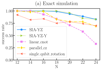
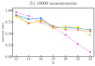
Figure 1: Success rate of CVaR-VQE with all parameters initialized as zero and $\alpha=0.01$ for (a) exact state vector simulation and (b) a noise-free quantum device with 10000 measurements in every iteration. The green dot and yellow triangle are the SIA ansatz; the pink square is the HEA with linear CNOT as the entanglement layer; the orange diamond is the HEA with CZ gate as the entanglement layer; the red triangle is the single-qubit-rotation ansatz only produce product states.

Figure 1, shows the success rate of the two variants of the SIA introduced above compared to various ansätze that haven been widely used in the literature. In particular, we compare the SIA variants to HEAs with linear CNOT entanglement, parallel CZ entanglement and a single-qubit rotation ansatz that produces only product states (see Appendix B, Figs. 11(a) - 11(c) for details). For a fair comparison, all the ansätze were applied to the same initials state, the uniform superposition state $\ket{+}^{\otimes N}$, with the same number of parameters $N^{2}$ and all parameters set to zero initially, as detailed in Appendix. B. Note that we have not introduced the warm start for SIA yet. Focusing on the results obtained from the exact simulation in Fig. 1(a), corresponding to a perfect noise-free quantum computer with an infinite number of measurements, the SIA ansätz shows a slightly higher success rate than the other ansätze, in particular for large problem sizes. The HEA ansatze with linear CNOT entangling layers performs only better than the single-qubit rotation ansatz without any entanglement for the problems with less than 18 qubits. From there on they are worse (HEA with linear CNOT entangling layers) or on par (HEA with parallel CZ entangling layers) with the single-qubit rotation ansatz.

Incorporating the fact that actual quantum devices only allow for a finite number of measurements changes the picture significantly, as Fig. 1(b) reveals. Despite using a relatively large number of 10000 measurements per iteration, the statistical noise leads to a significant drop in performance of the SIA ansätze. In particular, they lose their advantage over the single-qubit rotation ansatz, and except for the HEA with linear CNOT entangling layers, all variational ansätze show very similar performance for the entire range of problem sizes we study. Our results are in agreement with the conclusion of Ref. Díez-Valle et al. (2021), which found that entanglement gates adapted to the problem structure are beneficial for optimization problems while the advantage will decrease in the case of a finite number of measurements. The poor performance of HEA and SIA at large problem sizes with a finite number of measurements might be the result of statistical errors as well as barren plateaus, which will be further discussed in Sec. VI.

Notice that both the ansatz SIA-YZ and SIA-YZ-Y show a compatible performance in the exact simulation as well as a finite number of measurements, hence we will predominantly concentrate on the SIA-YZ ansatz in the following analyses. While these initial results indicate the SIA loses its advantage in success rate with a finite $S$, we discuss a warm start procedure for the SIA in the following section. As we are going to demonstrate, the warm start approach is able to improve the performance significantly and allows for obtaining good results in the entire range of problem sizes we study with a finite number of measurements.

IV Warm start

In order to improve the performance of SIA with a finite number of measurements, we propose a strategy to provide a good initial guess for the parameters in the ansatz. Our approach is based on choosing the parameters such that the ansatz mimics ITE. As discussed in Sec. III, the effect of the single-body part of the imaginary time evolution operator can be realized up to normalization by $R_{y}$ rotation gates, with appropriately chosen parameters (see Eq. (6)).

Similarly, we can proceed with the two-body part of the ITE. However, since we have chosen a particular form for the two-qubit gates in the ansatz, these might not be able to exactly replicate the action of the two-body part of the imaginary time-evolution operator. In order to approximate the effect of $e^{-\tau J_{ij}\sigma_{i}^{z}\sigma_{j}^{z}}$ in Eq. (7) as well as possible with our ansatz, we can impose that the overlap between the state evolved in imaginary time and our SIA-YZ ansatz,

$$f_{\tau,k}(\theta_{ij,0},\theta_{ij,1})$$ (12)

$$=\bra{\psi_{k-1}}e^{-\tau\cdot J_{ij}\cdot\sigma_{i}^{z}\sigma_{j}^{z}}\cdot e^{-i(\theta_{ij,1}\cdot\sigma_{i}^{z}\sigma_{j}^{y}+\theta_{ij,0}\cdot\sigma_{i}^{y}\sigma_{j}^{z})/2}\ket{\psi_{k-1}},$$

is maximized. The above formula above corresponds to the expectation value of a two-qubit operator, which can be expanded as a sum of strings of two Pauli operators $\hat{P}\in\{I,\sigma^{x},\sigma^{y},\sigma^{z}\}^{\otimes 2}$, and the expectation $\bra{\psi_{k-1}}\hat{P}\ket{\psi_{k-1}}$ of the individual Paul strings can be measured efficiently. As detailed in Appendix A, after obtaining the expectation value of those Pauli operators, the overlap $f_{\tau,k}$ for a fixed time $\tau$ only depends on the parameters $\theta_{ij,0},\theta_{ij,1}$. The optimal parameters to maximize this overlap function can be easily found classically by solving

$$\theta_{ij,0}^{\ast},\theta_{ij,1}^{\ast} =\text{arg\ max}\ f_{\tau,k}(\theta_{ij,0},\theta_{ij,1}).$$ (13)

The new wave function for the next step is then given by $\ket{\psi_{k}}=U_{ij}(\theta_{ij,0}^{\ast},\theta_{ij,1}^{\ast})\ket{\psi_{k-1}}$.

Following this step, we progress to the subsequent pair of qubits and proceed in a similar manner. Based on the state $\ket{\psi_{k}}$, we estimate the overlap function $f_{\tau,k+1}$, and determine the optimal parameters by maximizing $f_{\tau,k+1}$. Iterating this process for all process for all qubits pairs with non-zero $J_{ij}$ in the Hamiltonian, we can obtain a set of parameters creating a state having significantly higher fidelity with the solution compared to the uniform superposition. Thus, the parameters determined this way, can serve as a warm start of the VQE. For the rest of the paper, we dub the method discussed above warm start by measuring, to distinguish it from the approximate warm start technique proposed in the next section.

Note that in general the warm start by measuring will only provide an approximation to the ITE. Since we have chosen a specific ansatz structure for the two-qubit gates, it will not be able to approximate the effect of the imaginary time evolution operator up to arbitrarily large $\tau$. For intermediate values of $\tau$ we expect that the warm start by measuring approach to provide a good initial state for the VQE.

Figure 2 demonstrates the efficiency of our warm start approach, by showing the fidelity of the state with initial parameters according to the warm start by measuring procedure compared to the uniform superposition.

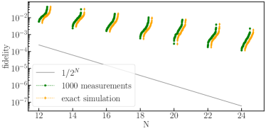
Figure 2: Fidelity of the warm start state that mimicking ITE with $\tau=0.2$. The yellow diamonds represents the initial state following the warm start by measuring technique using a state vector simulation, corresponding to an infinite number of measurements when estimating the expectation values. The green dots correspond to the data obtained using 1000 measurements for estimating each of the local Pauli operators. For each system size, the fidelity of 100 random QUBO problems are presented, sorted in ascending order and slightly offset on the $x$-axis for viewer convenience. The gray line shows the fidelity between the solution and the uniform superposition.

Across all random QUBO instances we study, the warm start consistently achieves a significantly higher fidelity than the uniform superposition. Besides, using a modest budget of 1000 measurements to estimate the expectation value of the local Pauli operators in Eq. (12), the simulated data taking into account a finite number of measurements is close to the exact state vector simulation. Remarkably, this consistency does not decay with the number of qubits, which indicates the necessary number of measurements does almost not increase with the number of the qubits for the entire range of problem sizes we consider. This is likely because the warm start by measuring only requires the estimation of expectations of two-qubit operators.

To show that the warm start by measuring not only increases the fidelity of the initial state with the exact solution, but generally also leads to a better VQE performance, we show the success rate and the average number of iterations until reaching a certain fidelity threshold in Fig. 3.

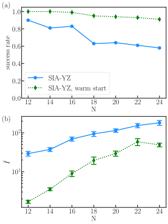
Figure 3: (a) Success rate of CVaR-VQE with $\alpha=0.01$ for warm start and (b) the averaged iterations to achieve the fidelity threshold $1\%$, with the errorbar representing the standard error. In both panels, the green diamond represents the data using the warm start by measuring with $\tau=0.2$, and in comparison, the blue dots represent the results using the uniform superposition as the initial state of VQE. The number of measurements for the warm start parameter estimation is 1000, and 10000 measurements are used for estimating the CVaR value in each VQE iteration for both cases with or without the warm start.

Focusing on the success rate in Fig. 3(a) first, it shows that the VQE with a finite number of measurements initialized with the warm start parameters has a much higher success rate compared to starting VQE with the uniform superposition state with all parameters set to zero. The separation in success rate between both cases grows slightly as the problem size increases. In addition, for the successful instances, we also record the minimal number of iterations to achieve the fidelity threshold $1\%$. Figure 3(b) shows the average number of iterations, $\bar{I}$, among the successful instances to reach the desired fidelity threshold. As the figure reveals, $\bar{I}$ is noticeably smaller when using the warm start by measuring, indicating a faster convergence rate of the VQE with warm start parameters towards the optimal solution. Specifically, for 24 qubits, $\bar{I}$ of VQE without warm start is around $180$, whereas with warm start, it reduces to about $50$, thus achieving the fidelity threshold up to 3.6 times more rapidly.

V Warm start without measurements

The warm start by measuring approach allows for improving the performance of the VQE using $\text{CVaR}_{\alpha}$, as we have demonstrated in the last section However, this comes at the expense of having to perform additional measurements. Here we demonstrate an approximate way for warm starting the VQE. As the analysis in Appendix A shows one finds for the expectation values of the different Pauli operators

$$\bra{\psi_{k-1}}\hat{P}\ket{\psi_{k-1}}=\ ^{N\otimes}\bra{+}\hat{P}\ket{+}^{\otimes N}+\mathcal{O}(\tau^{2}).$$ (14)

Hence, provided $\tau$ is small, this allows for the approximating the warm start parameters by evaluating the expectation values of Pauli operators $\hat{P}$ in the state $\ket{+}^{\otimes N}$. These can be obtained analytically, and evaluate either to $0$ or $\pm 1$, so that an approximation of the warm start parameters can be obtained without running the quantum circuit. Hence, we dub this technique warm start by approximation. As Fig. 4 shows, for values of $\tau\leq 0.3$, the warm start by approximation yields fidelities with the exact solution comparable to those of the warm start by measuring discussed previously.

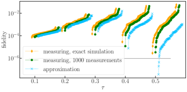
Figure 4: Comparision of warm start fidelity between warm start by measure and by approximation methods with 20 qubits. The fidelity of the warm start by measuring method introduced in Sec. IV, is presented by the yellow diamond for state vector simulation and green dots for simulation with 1000 measurement. The fidelity resulting from the warm start by approximation method is denoted by blue crosses. The gray line represents the fidelity of the uniform superposition which is $1/2^{20}$.

Only for larger values of $\tau$, the fidelity of the state initialized with warm start by approximation decreases, which can be attributed to the increasing error term $\mathcal{O}(\tau^{2})$ in estimating the expectation value of Pauli operators using state $\ket{+}^{\otimes N}$. Further comparisons between these two warm start approaches, in particular, for a larger number of ansatz layers are presented in Appendix C, revealing the warm start by measuring approach has a more stable performance using a larger number of layers.

In Fig. 5, we show the success rate of the VQE initialized with the warm start parameters derived from different approaches for $20$ qubits. This outcome exhibits a pattern consistent with that observed in Fig. 4: the success rate for the warm start by measuring approach with 1000 measurements is on par with that of infinite shots, and the approximation approach has a comparable performance when $\tau$ is small, but performs worse when $\tau$ increasing. Subsequent sections will focus on $\tau=0.2$, where both warm start by measure and by approximation methods show promising performance with a single layer. For stable performance across different layers, we will use the warm start by measuring method to generate good initial parameters for VQE.

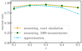
Figure 5: Success rate of CVaR-VQE with $\alpha=0.01$ initiated with different warm start parameters for 20 qubits. Each VQE iteration involved 10,000 measurements for estimating CVaR across all three warm start approaches

As our results demonstrate, for a single layer there is essentially no difference in performance between the different warm start approaches, and for the following section, we sill simply focus on the approach warm start by measuring.

VI Effects of statistical errors and resilience to barren plateaus

To elucidate the underlying factors contributing to the efficacy of the warm start strategy, we study the impact of statistical errors arising from a finite number of measurements. In addition, we investigate the gradients using the warm start to determine its resilience to barren plateaus.

VI.1 Statistical errors due to a finite number of measurements

To study the effect of a finite number of measurements, we utilize the QUBO instances with 18 qubits as a test bed. For these instances, the ideal simulation of the VQE, i.e. using an infinite number of measurements, with $\text{CVaR}_{0.01}$ as a cost function shows success rates for the SIA-YZ ansatz with and without warm start close to $100\%$ ($99\%$ for all initial parameters set to zero, $100\%$ for warm start). Thus, this setting serves as a testbed for analyzing how statistical errors influence success rates in each methodology.

Figure 6(a) illustrates how the success rate varies with the number of measurements used in every iteration, clearly indicating that the VQE with a warm start is more robust against the finite shots.

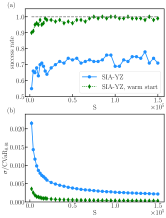
Figure 6: Scaling of the success rate of the CVaR-VQE with $\alpha=0.01$ (a) and relative standard error (b) for 18 qubits with averaged over 100 QUBO instances. The $x$-axis represents different numbers of measurements taken for determining the cost function in each iteration, ranging from 2000 to 150000. The blue dots represent the data for the VQE with the SIA-YZ ansatz initialized with the uniform superposition state, the green diamonds the results for initializin the ansatz using the warm start parameters. The grey dashed line in panel (a) indicates a success rate $100\%$.

Using the warm start, one consistently observes success rates close to $100\%$ as soon as the number of measurements is larger than 70000. Even for as little as 2000 measurements, one can achieve a high success rate of $90\%$. In contrast, the VQE without a warm start achieves only maximum success rates of approximately $70\%$, even for 150000 measurements. To obtain further insight into the mechanism behind the robustness of the warm start, we calculate the standard error of the expectation value for the cost function $\text{CVaR}_{\alpha}$ with coefficient $\alpha$ and a number of measurements $S$. The standard error is given by

$$\sigma=\sqrt{\frac{\sum_{k=1}^{\lceil\alpha\cdot S\rceil}\left(E_{k}-\text{CVaR}_{\alpha}(E)\right)^{2}}{\lceil\alpha\cdot S\rceil\left(\lceil\alpha\cdot S\rceil-1\right)}},$$ (15)

where $\alpha=0.01$ in this study and the obtanined from each of the measurements are sorted in ascending order: $E_{1}\leq E_{2}\leq\cdots\leq E_{S}$. A larger standard error indicates greater uncertainty in $\text{CVaR}_{0.01}$ when estimating the cost function with finite number of measurements. This might mislead the classical optimizer when selecting the a new set of parameters to minimize the cost function value. The relative standard error $\sigma/\text{CVaR}_{0.01}$ of the 10th iteration in VQE is plotted in Fig. 6(b), demonstrating that the standard error is significantly reduced when utilizing a warm start. This might explain the improved performance of the warm start with a finite measurements. In turn, the reduced standard error is as a result of the warm start procedure mimicking the ITE initially pushing more weights into the low-energy states, resulting in a more concentrated lowest-$\alpha$ tail of the measured eigenvalue distribution.

VI.2 Resilience to barren plateaus

The problem of barren plateaus is one of the most difficult problems for the VQE, as it can prevent the trainability of ansätze McClean et al. (2018). Thus, it is pertinent to investigate if the SIA ansatz and warm start can mitigate this problem. To this end, we examine the scaling of the cost concentration with the number of qubits for the SIA ansatz, which was proven to be exponentially decaying if the cost landscape has the problem of barren plateaus Arrasmith et al. (2022).

To study to what extent the SIA-YZ ansatz is affected by barren plateaus with increasing circuit depth, we consider the ansatz with a number layers $L\geq 1$ which is given by

$$\prod_{l=1}^{L}\left(\prod_{(i,j)\in E}U_{ij}(\bm{\theta}_{ij}^{l})\times\prod_{i\in V}R_{y}(\theta_{i}^{l})\right)\ket{+}^{\otimes N}.$$ (16)

Furthermore, in this section, besides $\alpha=0.01$, we also consider the $\alpha=0.1$, because some instances for $N=12,14,16$ might gain fidelity larger than $0.01$ in the warm start, where the global minimal is already achieved for $\alpha=0.01$, resulting in zero gradient. This could cause an increase in gradient as the number of qubits increases, so we also consider $\alpha=0.1$ to verify the scaling of the gradients with the problem size.

Firstly, we explore the variance of the cost difference with increasing number of ansatz layers. For each random QUBO instance and each number of layers $L$, we sample 2000 random parameter vectors, $\bm{\theta}=\{\theta_{i}^{l},\bm{\theta}_{jk}^{l}|i\in V,(j,k)\in E,1\leq l\leq L\}$, and evaluate the variance of the cost difference as in Eq. (13) in Ref. Arrasmith et al. (2022)

$$\text{Var}(\Delta C)=\text{Var}_{\bm{\theta}}[C(\bm{\theta})-\mathbb{E}_{\bm{\theta}}[C(\bm{\theta})]].$$ (17)

As throughout the rest of the paper, the cost function $C(\bm{\theta})$ is given by the CVaR_α in Eq. (3).

The numerical simulation result is shown in Fig. 7. As the depth of a single layer of our ansatz circuit depends on the number of qubits $N$, we show $\text{Var}(\Delta C)$ as a function of circuit depth for better comparability of results for different problem sizes. Looking at Fig. 7, we initially observe an exponential decay, before reaching a plateau at $L\geq 2$. This indicates the SIA-YZ ansatz will form a unitary 2-design upon reaching sufficient depth McClean et al. (2018). In addition, we observe that the value of the plateau reached for a fixed problem size decays exponentially with the number of qubits $N$. Our results indicate that the SIA-YZ generally shows barren plateaus as $L$ increases.

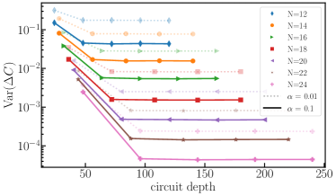
Figure 7: Cost concentration of the SIA-YZ ansatz for an even number of qubits ranging from 12 to 24. For each problem size, the value of $\text{Var}(\Delta C)$ is averaged over 10 random instances. The $x$-axis represents the circuit depth (layers of CNOT gates), which equals $2NL$ if considering an all-to-all connected hardware, as explained in Appendix B.

Furthermore, we also study the gradient observed using the warm start. Note that in the case of $l\geq 2$, the parameters of single-qubit gates in the warm start by measuring approach should also be determined by maximizing the overlap function similar to Eq. (12), because the state they are acting on is no longer a product state anymore. To facilitate a direct comparison with the cost concentration, which correlates with the gradients’ variance, we explore the squared gradient values normalized by the dimension of the parameter space, $\text{dim}(\bm{\theta})$, for a given instance

$$G=\frac{1}{\text{dim}(\bm{\theta})}\sum_{i=1}^{\text{dim}(\bm{\theta})}\left(\partial_{i}C(\bm{\theta})\right)^{2}.$$ (18)

The data for $G$ are shown in Fig. 8 for various problem sizes. As the figure reveals, the gradient obtained using the warm start parameters is not decaying with an increasing number of qubits. In particular, for the smaller value of $\alpha=0.01$ we observe an increase in gradient magnitude. This can be primarily attributed to the high fidelity of the warm start for smaller system sizes. As we have shown in Fig. 2, for $N=12$ most instances have a fidelity exceeding $0.01$ using the warm start parameters. Thus, for $\alpha=0.01$ the cost function is essentially already optimal, and the gradient will be zero. As the number of qubits increases, the fidelity of the warm start eventually decreases below $\alpha$, leading to a nonvanishing gradient and, thus, to the observed increase in gradient magnitude, as can be seen in Fig. 8(a). For the data with $\alpha=0.1$, shown in Fig. 8(b), we observe essentially a constant value of the gradient throughout the entire range of system sizes we study. This is a result of the fact that in this case the warm start does not reach fidelities lager than $\alpha$ (see Fig. 2), and the cost function for smaller $N$ is not close to the optimal value. In both case, $\alpha=0.01$, $0.1$, increasing the number of layers in the ansatz from 1 to 2 will result in a better warm start, resulting in a smaller value of the gradient. However, increasing the number of layers further beyond 2 does not necessarily enhance fidelity and consequently not reduce the value of gradient further, explaining why the data for $L\geq 2$ is approximately the same for large $N$. In summary, initializing the ansatz using the warm start method does not lead to exponentially vanishing gradients, while naively increasing the number of layers will not improve the performance systematically.

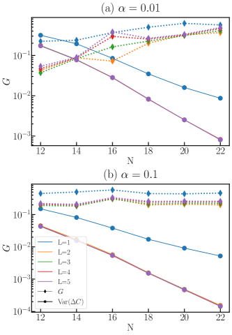
Figure 8: Scaling of the gradient obtained using the warm start parameters and cost concentration with the number of qubits, with (a) $\alpha=0.01$ and (b) $\alpha=0.1$. The dashed lines represent the square of the gradient for warm start parameters, and the solid lines represent the cost concentration. Different colors indicate different layers, and the cost concentration for $L\geq 2$ are degenerated in the plot.

The warm start provides a set of initial parameters with a large gradient, ensuring a trainable first step in the VQE. However, there are still questions about the trainability of subsequent iteration steps, and whether the warm start will lead the optimization to global or local minima. The high success rate and fast convergence to the optimal solution shown in Fig. 3 indicates that the warm start parameter should benefit these problems. To demonstrate this in a more straightforward way, we choose a random instance with $N=24$ qubits and a single ansatz layer to examine the optimization process of the VQE with different parameter initialization strategies, aiming to confirm the warm start provides a starting point that is easier to be optimized to the optimal solution. For simplicity, we only present the result of $\alpha=0.01$, The conclusions remain consistent for $\alpha=0.1$.

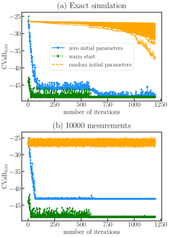
s

Figure 9: VQE process with different starting points of $L=1$. The $x$-axis represents the number of iterations and the $y$-axis represents the cost function value. Blue dots correspond to the VQE process starting at the uniform superposition state. The green diamonds represent that starting with the warm start. The orange dashed lines corresponds to VQE processes starting with 100 random initial parameters.

As shown in Fig. 9, a random choice of initial parameters essentially leads to an untrainable ansatz, especially in the case of using a finite number of measurements. Even with an exact state vector simulation (see Fig. 9 (a)), corresponding to an infinite number of measurements, most instances show barely any improvement of the cost function during the training process. The few instances that do show some improvement converge rather slow and stay far away from the minimum cost function value over the course of 1250 iterations. As soon as we use a finite number of measurements $S=10000$ (c.f. Fig. 9 (b)), we observe no substantial improvement of the cost function throughout the training process for randomly chosen initial parameters. This observation aligns with our findings on barren plateaus for the SIA-YZ ansatz discussed previously.

Initializing with all parameters being zero, corresponding to the uniform superposition as initial state, will result in a large gradient in the beginning, which enables the optimizer to quickly find a direction where the cost function decreases. However, even with an infinite number of measurements it takes a long time to get close to the global minimum and the optimization process is revolving around a local minimum for a long time, as Fig. 9(a) demonstrates. Using a finite number of measurements, Fig. 9(b) illustrates that this initialization tends to get stuck in local minima, explaining the low success rate observed previously in Fig. 1(b). This issue can be attributed to the large statical errors as discussed in Sec. VI.1.

In contrast, initializing parameters using the warm start method results in an initially already small value of the cost function, and the optimization procedure reliably converges to the optimal solution, in scenarios with both infinite and finite shots, as the results in Fig. 1 reveals. This indicates that our warm start is able to provide a good starting point in the cost function landscape that is close to the narrow gorges in which the cost function is concentrated and can help to overcome trainability issues.

VII Summary and outlook

In this work, we introduced a parametric ansatz suitable for addressing QUBO problems with VQE. The ansatz is inspired by the problem structure, and we proposed a novel, resource-efficient warm start method for it mimicking the evolution of the uniform superposition of all computational basis states in imaginary time. Performing classical simulations with up to $24$ qubits we numerically benchmarked the performance of the warm start for the VQE using the conditional value at risk as a cost function. Our data demonstrate that the warm start procedure allows for obtaining a good performance, even with a modest number of measurements per iteration in the VQE. The boost in performance through the warm start method can be primarily attributed to the fact that the initial state generated has a dominant component of low-energy states, resulting in a reduction of statistical errors when estimating expectation values with a finite number of measurements. Moreover, we also examined the resilience of the ansatz against barren plateaus. While we observe that the ansatz in general suffers from exponential cost concentration, our numerical results indicate that the warm start provides a point in parameter space sufficiently close to one of the narrow gorges where the cost function does not look flat.

It is worth mentioning that in our warm start approach, we determined the optimal parameter of each gate in the ansatz individually while keeping the others fixed to mimic the ITE. While this is the most resource-efficient approach in terms of overhead require for the warm start, optimizing multiple parameters of at the same time might allow for faithfully emulating the effect of imaginary time evolution up to longer time-scales. This could provide an initial state that has even larger overlap with the solution as our current technique. Evaluating the trade-off between the cost for obtaining good warm start parameters and the resulting performance enhancement in the subsequent VQE will be an interesting aspect for further subsequent studies.

Moreover, in our simulations considered an ideal quantum device performing a finite number of measurement. For the future it would be interesting to realize the simulation on current noisy quantum hardware and to investigate if the warm start shows a similar performance improvement in the presence of noise and in combination with state of the art error mitigation methods Endo et al. (2018); Cai et al. (2020); Funcke et al. (2022); van den Berg et al. (2022); Viola and Lloyd (1998). In addition, it is an interesting question different kinds of hardware noise affect the warm start procedure and how these could possibly be mitigated.

Appendix A Details of the warm start procedures

For the warm start by measuring approach, we have to maximize the expectation value in Eq. (12) by choosing appropriate variational parameters for the two-qubit gate acting on qubits $i$ and $j$. Utilizing the identities $e^{-a\hat{P}}=\cosh(a)-\sinh(a)\hat{P}$ and $e^{-ia\hat{P}}=\cos(a)-i\sin(a)\hat{P}$, for a real coefficient $a$ and $\hat{P}$ denoting one of the the Pauli operators, $\hat{P}\in\{I,\sigma^{x},\sigma^{y},\sigma^{z}\}^{\otimes 2}$, we can rewrite the overlap $f_{k}$ as follows

$$f_{\tau,k}(\theta_{ij,0},\theta_{ij,1})$$ (19)

$$=\bra{\psi_{k-1}}e^{-\tau\cdot J_{ij}\cdot\sigma_{i}^{z}\sigma_{j}^{z}}\cdot e^{-i(\theta_{ij,1}\cdot\sigma_{i}^{z}\sigma_{j}^{y}+\theta_{ij,0}\cdot\sigma_{i}^{y}\sigma_{j}^{z})/2}\ket{\psi_{k-1}}$$

$$=\cos\left(\frac{\theta_{ij,1}}{2}\right)\cos\left(\frac{\theta_{ij,0}}{2}\right)\left(\cosh\left(\tilde{\tau}_{ij}\right)-\sinh\left({\tilde{\tau}_{ij}}\right)\cdot\langle\sigma_{i}^{z}\sigma_{j}^{z}\rangle\right)$$

$$-i\cos\left(\frac{\theta_{ij,1}}{2}\right)\sin\left(\frac{\theta_{ij,0}}{2}\right)\left(\cosh\left(\tilde{\tau}_{ij}\right)\langle\sigma_{i}^{y}\sigma_{j}^{z}\rangle+i\sinh\left({\tilde{\tau}_{ij}}\right)\cdot\langle\sigma_{i}^{x}\rangle\right)$$

$$-i\sin\left(\frac{\theta_{ij,1}}{2}\right)\cos\left(\frac{\theta_{ij,0}}{2}\right)\left(\cosh(\tilde{\tau}_{ij})\langle\sigma_{i}^{z}\sigma_{j}^{y}\rangle+i\sinh\left({\tilde{\tau}_{ij}}\right)\cdot\langle\sigma_{j}^{x}\rangle\right)$$

$$-\sin\left(\frac{\theta_{ij,1}}{2}\right)\sin\left(\frac{\theta_{ij,0}}{2}\right)\left(\cosh\left(\tilde{\tau}_{ij}\right)\langle\sigma_{i}^{x}\sigma_{j}^{x}\rangle+\sinh\left({\tilde{\tau}_{ij}}\right)\cdot\langle\sigma_{i}^{y}\sigma_{j}^{y}\rangle\right).$$

In the above expression, we have used the short-hand notations $\tilde{\tau}_{ij}=\tau J_{ij}$ and $\langle\hat{P}\rangle=\bra{\psi_{k-1}}\hat{P}\ket{\psi_{k-1}}$. Notice that $\langle\sigma_{i}^{z}\sigma_{j}^{y}\rangle=0=\langle\sigma_{i}^{y}\sigma_{j}^{z}\rangle$, because these two operators are imaginary and hermitian, resulting in a vanishing expectation in a real state.

A similar calculation can be performed for the operators $\sigma_{i}^{x}\sigma_{j}^{y},\sigma_{i}^{y}\sigma_{j}^{x}$ in the ansatz, the corresponding overlap will be given by

$$f^{\prime}_{\tau,k}(\theta_{ij,0},\theta_{ij,1})$$ (20)

$$=\bra{\psi_{k-1}}e^{-\tau\cdot J_{ij}\cdot\sigma_{i}^{z}\sigma_{j}^{z}}\cdot e^{-i(\theta_{ij,1}\cdot\sigma_{i}^{x}\sigma_{j}^{y}+\theta_{ij,0}\cdot\sigma_{i}^{y}\sigma_{j}^{x})/2}\ket{\psi_{k-1}}$$

$$=e^{-\tilde{\tau}_{ij}}\cdot\left(\cos\left(\frac{\theta_{ij,1}}{2}\right)\cos\left(\frac{\theta_{ij,0}}{2}\right)-\sin\left(\frac{\theta_{ij,1}}{2}\right)\sin\left(\frac{\theta_{ij,0}}{2}\right)\cdot\langle\sigma_{i}^{z}\sigma_{j}^{z}\rangle\right).$$

This expression is maximized when $\theta_{ij,0}=0=\theta_{ij,1}$, which explains why we did not include the operator $\sigma_{i}^{x}\sigma_{j}^{y},\sigma_{i}^{y}\sigma_{j}^{x}$ in our ansatz.

Considering the expectation of the Pauli operators in Eq. (19), with operator $\hat{P}=\sigma_{i}^{x},\sigma_{j}^{x},\sigma_{i}^{x}\sigma_{j}^{x},\sigma_{i}^{y}\sigma_{j}^{y},\sigma_{i}^{z}\sigma_{j}^{z}$, the expectation $\langle\hat{P}\rangle$ can be expanded by using the definition of $\ket{\psi_{k-1}}$ from Eq. (7)

$$\langle\hat{P}\rangle =\bra{\psi_{k-1}}\hat{P}\ket{\psi_{k-1}}$$ (21)

$$=\bra{\psi_{k-2}}e^{i(\theta_{pq,1}\cdot\sigma_{p}^{z}\sigma_{q}^{y}+\theta_{pq,0}\cdot\sigma_{p}^{y}\sigma_{q}^{z})/2}\cdot\hat{P}\cdot e^{-i(\theta_{pq,1}\cdot\sigma_{p}^{z}\sigma_{q}^{y}+\theta_{pq,0}\cdot\sigma_{p}^{y}\sigma_{q}^{z})/2}\ket{\psi_{k-2}}$$

$$=\bra{\psi_{k-2}}\hat{P}\ket{\psi_{k-2}}+\bra{\psi_{k-2}}i\left[\sigma_{p}^{z}\sigma_{q}^{y}+\sigma_{p}^{y}\sigma_{q}^{z},P\right]\ket{\psi_{k-2}}\cdot\mathcal{O}(\tau)+\mathcal{O}(\tau^{2}),$$

$$=\ ^{N\otimes}\bra{+}\hat{P}\ket{+}^{\otimes N}+\left(\sum_{i\in V}\ ^{N\otimes}\bra{+}i\left[\sigma_{i}^{y},P\right]\ket{+}^{\otimes N}+\sum_{pq\in E^{\prime}}\ ^{N\otimes}\bra{+}i\left[\sigma_{p}^{z}\sigma_{q}^{y}+\sigma_{p}^{y}\sigma_{q}^{z},P\right]\ket{+}^{\otimes N}\right)\cdot\mathcal{O}(\tau)+\mathcal{O}(\tau^{2})$$

$$=\ ^{N\otimes}\bra{+}\hat{P}\ket{+}^{\otimes N}+\mathcal{O}(\tau^{2}).$$

In the second line of the above equation, qubits indexed by $p,q$ refer to the gate applied at step $k-1$. The Baker-Campbell-Hausdorff formula, $e^{\hat{A}}\cdot\hat{P}\cdot e^{-\hat{A}}=\hat{P}+[\hat{A},\hat{P}]+\frac{1}{2}[\hat{A},[\hat{A},\hat{P}]]\cdots$, was used for the expansion on the third line. Besides, it is assumed that the parameters $\theta_{pq,0}$ and $\theta_{pq,1}$ are of the same order as $\tau$. Finally, all gates existing in the circuit before step $k$ are expanded in a similar procedure. $E^{\prime}$ represents the pairs of two-qubit gates that were previously applied in the circuit, with $(p,q)\in E^{\prime}$ being different from $(i,j)$, such that the commutator $\left[\sigma_{p}^{z}\sigma_{q}^{y}+\sigma_{p}^{y}\sigma_{q}^{z},P\right]$ will be zero or contain $\sigma^{z}$ or $\sigma^{y}$ operator, resulting in a zero expectation in state $\ket{+}^{\otimes N}$, similar to the terms $\left[\sigma_{i}^{y},P\right]$. Therefore, the expectation $\langle\hat{P}\rangle$ can be estimated in the product state with the error $\mathcal{O}(\tau^{2})$ .

Appendix B Circuits for different ansätze

The circuit for the SIA-YZ ansatz includes two-qubit gates for all possible qubit pairs. In general, current hardware platforms only offer limited qubit connectivity, and we need additional SWAP gates to realize all-to-all connectivity. Following the strategy in Ref. Weidenfeller et al. (2022), we take 6 qubits as an example and show the resulting circuit assuming linear qubit connectivity in Fig. 10. Full connectivity is reached after $N-2$ SWAP layers, and the SWAP gate is compressed with the operator $U_{ij}(\bm{\theta}_{ij})^{YZ}$ in Eq. (11), thus they can be implemented with 3 CNOT gates (purple box in Fig. 10). Additionally, the first and final layers are only gates $U_{ij}(\bm{\theta}_{ij})^{YZ}\in SO(4)$ that can be decomposed by using 2 CNOT gates Vatan and Williams (2004) (green box in Fig. 10). Consequently, the overall structure requires $3N-2$ CNOT layers and $\mathcal{O}(1.5N^{2})$ CNOT gates. Alternatively, if the quantum device has all-to-all connectivity, no additional SWAP gates are necessary and the circuit only consists of the gates $U_{ij}(\bm{\theta}_{ij})^{YZ}$ and single-qubit rotation gates. In this case the circuit depth is reduced to $2N$ CNOT layers and $\mathcal{O}(N^{2})$ CNOT gates.

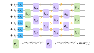
Figure 10: SIA circuit for 6 qubits. The yellow number indicates the qubit index after the SWAP operation.

In addition to the SIA, we consider three alternative ansätze often used in the literature for comparison, which are illustrated in Fig. 11. For a fair comparison, all ansätze have the same number of parameters, utilizing $N^{2}$ parameters equivalent to those of a single-layer SIA, thereby necessitating $N$ layers for the ansatz depicted in Fig. 11. Moreover, Table 1 shows the number of two-qubit gates required for each ansatz, maintaining the same parameter count as the 1-layer SIA.

(a)  Hardware-efficient ansatz with linear CNOT entanglement.

(b)  Hardware-efficient with parallel CZ entanglement.

(c)  Single-qubit-rotation ansatz

Figure 11: Different ansätze used for comparison with the SIA. Panel (a) shows the hardware-efficient ansatz producing real amplitudes with linear CNOT entangling layers, panel (b) the same ansatz but with non-overlapping, parallel CZ entangling layers and panel (c) an ansatz consisting of single-qubit gates only, thus not being able to generate any entanglement.

	SIA	HEA with linear CNOT	HEA with parallel CZ	Single-qubit rotations
linear	$1.5N^{2}-2.5N+1$	$(N-1)^{2}$	$(N-1)^{2}$	0
all-to-all	$N(N-1)$	$(N-1)^{2}$	$(N-1)^{2}$	0

Table 1: Number of CNOT gates for different ansätze with $N^{2}$ parameters, with respect to linear or all-to-all qubit connectivity of the hardware platform.

Appendix C Performance of the warm start approach for more than a single layer

This appendix shows results for the performance of the warm start across different number of layers, $L=1,2,3,4,5$. Figure 12 shows the data for 20 qubits as an example and compares the fidelity between the warm start by measuring and warm start by approximation. While both approaches yield comparable results for a single layer, the fidelity achieved through the warm start by approximation decreases with an increasing number of layers. Conversely, the warm start by measuring method maintains a relatively consistent performance for all values of $L$ we consider. Notably, the fidelity improves slightly when going from a single layer to $L=2$, but there is no significant improvement when further adding additional layers. This observation suggests the necessity to incorporate more non-local operators if one wants to enhance the fidelity of the initial state with the exact solution.

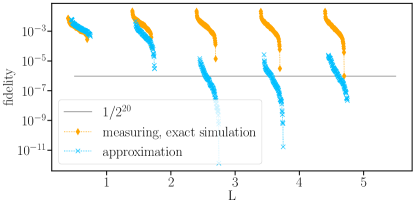
Figure 12: Fidelity of warm start by measuring and warm start by approximation methods using a state vector simulation for 20 qubits for different numbers of layers, $\tau=0.2$ is used for all data points.

References

- Peruzzo et al. (2014) Alberto Peruzzo, Jarrod McClean, Peter Shadbolt, Man-Hong Yung, Xiao-Qi Zhou, Peter J Love, Alán Aspuru-Guzik, and Jeremy L O’brien, “A variational eigenvalue solver on a photonic quantum processor,” Nat. Commun. 5, 1–7 (2014).
- Cerezo et al. (2021) Marco Cerezo, Andrew Arrasmith, Ryan Babbush, Simon C Benjamin, Suguru Endo, Keisuke Fujii, Jarrod R McClean, Kosuke Mitarai, Xiao Yuan, Lukasz Cincio, et al., “Variational quantum algorithms,” Nat. Rev. Phys. 3, 625–644 (2021).
- Meglio et al. (2023) Alberto Di Meglio, Karl Jansen, Ivano Tavernelli, Constantia Alexandrou, Srinivasan Arunachalam, Christian W. Bauer, Kerstin Borras, Stefano Carrazza, Arianna Crippa, Vincent Croft, Roland de Putter, Andrea Delgado, Vedran Dunjko, Daniel J. Egger, Elias Fernandez-Combarro, Elina Fuchs, Lena Funcke, Daniel Gonzalez-Cuadra, Michele Grossi, Jad C. Halimeh, Zoe Holmes, Stefan Kühn, Denis Lacroix, Randy Lewis, Donatella Lucchesi, Miriam Lucio Martinez, Federico Meloni, Antonio Mezzacapo, Simone Montangero, Lento Nagano, Voica Radescu, Enrique Rico Ortega, Alessandro Roggero, Julian Schuhmacher, Joao Seixas, Pietro Silvi, Panagiotis Spentzouris, Francesco Tacchino, Kristan Temme, Koji Terashi, Jordi Tura, Cenk Tuysuz, Sofia Vallecorsa, Uwe-Jens Wiese, Shinjae Yoo, and Jinglei Zhang, “Quantum computing for high-energy physics: State of the art and challenges. summary of the qc4hep working group,” (2023), arXiv:2307.03236 [quant-ph] .
- Tilly et al. (2022) Jules Tilly, Hongxiang Chen, Shuxiang Cao, Dario Picozzi, Kanav Setia, Ying Li, Edward Grant, Leonard Wossnig, Ivan Rungger, George H. Booth, and Jonathan Tennyson, “The variational quantum eigensolver: A review of methods and best practices,” Physics Reports 986, 1–128 (2022).
- Chai et al. (2023a) Yahui Chai, Lena Funcke, Tobias Hartung, Karl Jansen, Stefan Kühn, Paolo Stornati, and Tobias Stollenwerk, “Optimal flight-gate assignment on a digital quantum computer,” Phys. Rev. Appl. 20, 064025 (2023a).
- Chai et al. (2023b) Yahui Chai, Evgeny Epifanovsky, Karl Jansen, Ananth Kaushik, and Stefan Kühn, “Simulating the flight gate assignment problem on a trapped ion quantum computer,” (2023b), arXiv:2309.09686 [quant-ph] .
- Schwägerl et al. (2023) Tim Schwägerl, Cigdem Issever, Karl Jansen, Teng Jian Khoo, Stefan Kühn, Cenk Tüysüz, and Hannsjörg Weber, “Particle track reconstruction with noisy intermediate-scale quantum computers,” (2023), arXiv:2303.13249 [quant-ph] .
- Amaro et al. (2022) David Amaro, Matthias Rosenkranz, Nathan Fitzpatrick, Koji Hirano, and Mattia Fiorentini, “A case study of variational quantum algorithms for a job shop scheduling problem,” EPJ Quantum Technology 9 (2022), 10.1140/epjqt/s40507-022-00123-4.
- Nannicini (2019) Giacomo Nannicini, “Performance of hybrid quantum-classical variational heuristics for combinatorial optimization,” Phys. Rev. E 99, 013304 (2019).
- Scriva et al. (2024) Giuseppe Scriva, Nikita Astrakhantsev, Sebastiano Pilati, and Guglielmo Mazzola, “Challenges of variational quantum optimization with measurement shot noise,” Physical Review A 109 (2024), 10.1103/physreva.109.032408.
- McClean et al. (2018) Jarrod R. McClean, Sergio Boixo, Vadim N. Smelyanskiy, Ryan Babbush, and Hartmut Neven, “Barren plateaus in quantum neural network training landscapes,” Nature Communications 9 (2018), 10.1038/s41467-018-07090-4.
- Barkoutsos et al. (2020) Panagiotis Kl. Barkoutsos, Giacomo Nannicini, Anton Robert, Ivano Tavernelli, and Stefan Woerner, “Improving variational quantum optimization using cvar,” Quantum 4, 256 (2020).
- Kochenberger et al. (2014) Gary Kochenberger, Jin-Kao Hao, Fred Glover, Mark Lewis, Zhipeng Lü, Haibo Wang, and Yang Wang, “The unconstrained binary quadratic programming problem: a survey,” Journal of Combinatorial Optimization 28, 58–81 (2014).
- Hadfield (2021) Stuart Hadfield, “On the Representation of Boolean and Real Functions as Hamiltonians for Quantum Computing,” ACM Transactions on Quantum Computing 2, 18:1–18:21 (2021).
- Acerbi and Tasche (2002) Carlo Acerbi and Dirk Tasche, “On the coherence of expected shortfall,” Journal of Banking & Finance 26, 1487–1503 (2002).
- Díez-Valle et al. (2021) Pablo Díez-Valle, Diego Porras, and Juan José García-Ripoll, “Quantum variational optimization: The role of entanglement and problem hardness,” Phys. Rev. A 104, 062426 (2021).
- Motta et al. (2019) Mario Motta, Chong Sun, Adrian T. K. Tan, Matthew J. O’Rourke, Erika Ye, Austin J. Minnich, Fernando G. S. L. Brandão, and Garnet Kin-Lic Chan, “Determining eigenstates and thermal states on a quantum computer using quantum imaginary time evolution,” Nature Physics 16, 205–210 (2019).
- McArdle et al. (2019) Sam McArdle, Tyson Jones, Suguru Endo, Ying Li, Simon C. Benjamin, and Xiao Yuan, “Variational ansatz-based quantum simulation of imaginary time evolution,” npj Quantum Information 5, (2019).
- Sun et al. (2021) Shi-Ning Sun, Mario Motta, Ruslan N. Tazhigulov, Adrian T.K. Tan, Garnet Kin-Lic Chan, and Austin J. Minnich, “Quantum computation of finite-temperature static and dynamical properties of spin systems using quantum imaginary time evolution,” PRX Quantum 2, 010317 (2021).
- Yuan et al. (2019) Xiao Yuan, Suguru Endo, Qi Zhao, Ying Li, and Simon C. Benjamin, “Theory of variational quantum simulation,” Quantum 3, 191 (2019).
- Banks et al. (2024) Robert J. Banks, Dan E. Browne, and P.A. Warburton, “Rapid quantum approaches for combinatorial optimisation inspired by optimal state-transfer,” Quantum 8, 1253 (2024).
- Guan et al. (2023) Huijie Guan, Fei Zhou, Francisco Albarrán-Arriagada, Xi Chen, Enrique Solano, Narendra N. Hegade, and He-Liang Huang, “Single-Layer Digitized-Counterdiabatic Quantum Optimization for -spin Models,” (2023), arXiv:2311.06682 [quant-ph] .
- Powell (1994) Michael JD Powell, “A direct search optimization method that models the objective and constraint functions by linear interpolation,” in Advances in optimization and numerical analysis (Springer, 1994) pp. 51–67.
- Arrasmith et al. (2022) Andrew Arrasmith, Zoë Holmes, M Cerezo, and Patrick J Coles, “Equivalence of quantum barren plateaus to cost concentration and narrow gorges,” Quantum Science and Technology 7, 045015 (2022).
- Endo et al. (2018) Suguru Endo, Simon C. Benjamin, and Ying Li, “Practical quantum error mitigation for near-future applications,” Phys. Rev. X 8, 031027 (2018).
- Cai et al. (2020) Zhenyu Cai, Xiaosi Xu, and Simon C. Benjamin, “Mitigating coherent noise using pauli conjugation,” npj Quantum Information 6, 17 (2020).
- Funcke et al. (2022) Lena Funcke, Tobias Hartung, Karl Jansen, Stefan Kühn, Paolo Stornati, and Xiaoyang Wang, “Measurement error mitigation in quantum computers through classical bit-flip correction,” Phys. Rev. A 105, 062404 (2022).
- van den Berg et al. (2022) Ewout van den Berg, Zlatko K. Minev, and Kristan Temme, “Model-free readout-error mitigation for quantum expectation values,” Phys. Rev. A 105, 032620 (2022).
- Viola and Lloyd (1998) Lorenza Viola and Seth Lloyd, “Dynamical suppression of decoherence in two-state quantum systems,” Phys. Rev. A 58, 2733–2744 (1998).
- Weidenfeller et al. (2022) Johannes Weidenfeller, Lucia C. Valor, Julien Gacon, Caroline Tornow, Luciano Bello, Stefan Woerner, and Daniel J. Egger, “Scaling of the quantum approximate optimization algorithm on superconducting qubit based hardware,” Quantum 6, 870 (2022).
- Vatan and Williams (2004) Farrokh Vatan and Colin Williams, “Optimal quantum circuits for general two-qubit gates,” Physical Review A 69 (2004), 10.1103/physreva.69.032315.