Quantum collective motion of macroscopic mechanical oscillators

Collective phenomena in physics arise from interactions among numerous components within a complex system, giving rise to behaviors that cannot be mapped to those of the constituent parts [1]. This broad domain encompasses classical phenomena such as synchronization [2], and extends to the quantum realm with phenomena as superconductivity [3], Bose-Einstein condensation [4], super-radiance [5], and collective coupling enhancement [6]. Studying such phenomena in well-controlled artificial systems is advantageous, as it allows to simulate complex natural systems and even to unveil unexplored behaviors. Solid-state mechanical oscillators, which can be controlled via optomechanical coupling [7], have been theoretically proposed for investigating collective phenomena [8, 9, 10, 11]. However, experimental realizations [12, 13] have been impeded by the stringent requirement of having nearly degenerate mechanical oscillators. Here, we present the collective behavior of multiple nearly degenerate mechanical oscillators (a hexamer, i.e. a system comprising 6 mechanical oscillators) coupled to a common cavity in a superconducting circuit optomechanical platform [14]. We experimentally demonstrate that, upon increasing the optomechanical coupling rates, such a system undergoes a transition from individual mechanical oscillators to a collective mode, where its motion is comprised of equal amplitude and relative phase of the individual oscillators. Leveraging the finite non-degeneracy of mechanical frequencies and rapidly quenching the optomechanical couplings, we directly measure the amplitude and the relative phase of mechanical oscillators in the collective mode. We show that the coupling rate of this collective mode to the cavity enhances with the number of coupled oscillators, akin to a Tavis-Cummings system [6] and super-radiance of identical atoms [5]. By increasing the coupling rates even further, this collective mode enters the strong coupling regime with the cavity. We demonstrate sideband ground-state cooling [7] of the collective mode, achieving 0.4 quanta occupation. Moreover, we observe the quantum sideband asymmetry for this collective mode [15]. Observing collective optomechanical phenomena in the quantum regime provides the opportunity to study large-scale synchronization [10], investigation of topological phases of sound [11], and more broadly, achieving multi-partite phonon-phonon [16, 17] and photon-phonon [18] entanglement.

Understanding the collective dynamics of complex multimode systems stands as a cornerstone in physics [1], allowing to describe fundamental emergent phenomena spanning phase transitions [19], spontaneous synchronization [2], and chaotic evolution [20]. These effects are particularly pronounced in quantum mechanics, where collective dynamics engender phenomena such as Bose-Einstein condensation [4], superconductivity [3], and superfluidity [21]. A notable collective phenomenon is the super-radiance of identical atoms [5], with applications in making narrow linewidth lasers [22]. Similarly, the collective enhancement of light-matter interaction in Tavis-Cummings systems [6], where multiple identical emitters are equally coupled to a common cavity, exemplifies the remarkable nature of collective phenomena. While atomic ensembles have historically been the natural testbed for studying collective phenomena [23, 24], recent efforts have expanded to engineered artificial atoms, such as superconducting [25, 26] or semiconducting [27, 28] qubits. The versatility in engineering light-matter interactions and transition spectra of these artificial systems offer new avenues for exploring collective behaviors.

Solid-state mechanical oscillators, although different in nature from two-level systems, are attractive artificial elements because of their compact footprint, long lifetimes, selective controllability, and low cross-talk. Controlling the quantum state of a macroscopic mechanical oscillator has become possible by employing either optomechanical coupling to an electromagnetic resonator [7] or piezoelectric coupling to superconducting qubits [29]. The former approach has led to landmark experimental achievements, including the sideband cooling of a mechanical oscillator to its ground state [30, 31], strong coupling [32, 33], and ponderomotive squeezing of light [34], even at room temperature [35]. Among all possible platforms, optomechanical systems based on superconducting circuits [14] have attracted considerable attention, primarily due to the ultralow quantum decoherence of their mechanical elements, maintaining sufficient optomechanical coupling, and residing in the resolved-sideband regime [36]. This architecture has successfully demonstrated ground state cooling [14] and squeezing [37, 36] of a mechanical oscillator, entanglement among macroscopic oscillators [38, 39], non-reciprocity [40], and mechanical quantum reservoir engineering [41], among numerous other optomechanical phenomena. Recent implementation of topological lattices using such superconducting circuit optomechanical systems [42] have laid the foundation for studying the collective behavior of mechanical oscillators.

Observing collective phenomena in optomechanical systems requires identical mechanical oscillators. Investigations into systems with degenerate mechanical oscillators have revealed long-range interactions [8, 9], hybridization [43], emergence of mechanical dark and bright modes [12, 13, 44], synchronization of the mechanical oscillators [10, 45], and topological phases of sound and light [11]. Interestingly, degeneracy in a non-Hermitian optomechanical system gives rise to exceptional points that exhibit different behavior than those of a Hermitian system [46, 47, 48, 49]. Despite these rich physical phenomena, experimental demonstrations of collective behaviors have been challenging and have been limited to just two nearly degenerate mechanical oscillators [12, 13, 43] or modes of a bulk-acoustic-wave resonator [44]. Collective phenomena, however, typically scale with the number of units involved, highlighting the importance of large-scale arrays of identical oscillators. This limitation primarily stems from imperfections in the fabrication process of mechanical elements.

Here we analyze theoretically and demonstrate experimentally the behavior of $N=6$ nearly degenerate mechanical oscillators, i.e. a mechanical hexamer, coupled to a shared microwave resonator, implemented in a superconducting circuit optomechanical platform [14, 36]. By optimizing the circuit design and fabrication process, we achieve a low level of mechanical frequency disorder, amounting to only 0.1%. This low disorder, together with mechanical quality factors with an average of $11\times 10^{6}$, enable the mechanical oscillators to undergo a transition from an individual behavior to a collective behavior as their optomechanical coupling rates increase, leading to the appearance of a bright and ($N-1$) dark mechanical collective modes. The bright collective mode ultimately reaches the strong coupling regime with the microwave resonator. Interestingly, the zero point motion of this collective mode is distributed over several physically distinct mechanical oscillators. As the bright collective mode emerges, we observe a $\sqrt{N}$-enhancement in its optomechanical coupling rate, akin to the coupling enhancement in the Tavis-Cummings Hamiltonian [6, 25, 26, 27, 28]. By quenching of the optomechanical coupling rates, we directly measure the amplitude and relative phase of the collective modes. We demonstrate sideband ground-state cooling, achieving a phononic occupation of 0.4 quanta for the bright collective mode, while the other dark collective modes retain larger phonon occupations. We are equally able to observe quantum sideband asymmetry [15] for the bright collective mode.

Nearly-degenerate mechanical oscillators

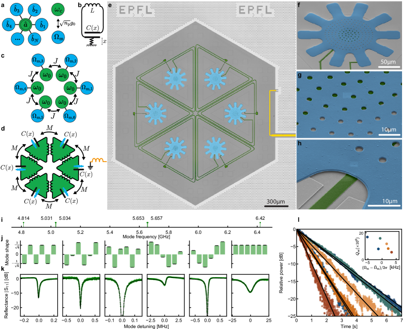
Figure 1: An optomechanical hexamer to study collective phenomena. a, Mode diagram for a general system composed of $N$ mechanical oscillators (in blue) optomechanically coupled to a cavity mode (in green). b, Circuit equivalent representation of a single optomechanical system, where a mechanical oscillator modulates the capacitance $C(x)$ of an $LC$ resonator. c, Mode diagram and d equivalent electrical circuit consisting of mechanically compliant vacuum gap capacitors: six identical optomechanical unit cells are coupled with rotational symmetry. A waveguide is inductively coupled to drive the system. e, False colour optical micrograph showing the device with details of the drum in f, g, and h. i, j, and k, The microwave mode frequencies, modeshapes, and reflection traces $|S_{11}|$, respectively. l, The ringdown measurements of the mechanical oscillators and their quality factors versus their frequencies in inset.

We aim to theoretically and experimentally study the role of degeneracy in optomechanical systems, comprising $N$ resonant mechanical oscillators $\hat{b}_{i}$ with frequency $\Omega_{{\rm m}}$ optomechanically coupled with equal coupling rates $g$ to a common photonic mode $\hat{a}$ with frequency $\omega_{\rm c}$, as depicted in Fig. 1a. The linearized Hamiltonian of the system in the presence of a pump with frequency $\omega_{\rm p}$ red-detuned from the cavity by $\Delta=\omega_{\rm c}-\omega_{\rm p}=\Omega_{\rm m}$ in the rotating frame of the pump is given by: $\hat{H}/\hbar=\Delta\hat{a}^{\dagger}\hat{a}+\Omega_{\rm m}\sum_{i=1}^{N}\hat{b}_{i}^{\dagger}\hat{b}_{i}+g\left(\hat{a}^{\dagger}\sum_{i=1}^{N}\hat{b}_{i}+\hat{a}\sum_{i=1}^{N}\hat{b}_{i}^{\dagger}\right)$. The optomechanical coupling rate $g=\sqrt{n_{\rm p}}g_{0}$ can be tuned by changing the intra-cavity photon number $n_{\rm p}$, where $g_{0}$ is the single photon optomechanical coupling rate.

The Hamiltonian can be recast into an effective beam-splitter interaction between the microwave mode and a single mechanical mode $\hat{\beta}_{1}=\frac{1}{\sqrt{N}}\sum_{i=1}^{N}\hat{b}_{i}$, that will be referred to as a bright collective mode from now on,

$$\hat{H}/\hbar=\Delta\hat{a}^{\dagger}\hat{a}+\Omega_{\rm m}\sum_{i=1}^{N}\hat{\beta}_{i}^{\dagger}\hat{\beta}_{i}+g\sqrt{N}\left(\hat{a}^{\dagger}\hat{\beta}_{1}+\hat{a}\hat{\beta}_{1}^{\dagger}\right),$$ (1)

while other collective modes $\hat{\beta}_{i\neq 1}$ are decoupled from the cavity, referred to as dark collective modes from now on. Notably, such decomposition is only possible due to the degeneracy of the mechanical oscillators, see Supplementary Information (SI). The bright collective mode $\beta_{1}$ is at the center of our investigation: its modeshape is characterized by equal participation and zero relative phase of each individual mechanical oscillator.

In contrast to the case of individual mechanical oscillators, the optomechanical interaction part in the Hamiltonian (1) includes an additional factor of $\sqrt{N}$. This collective enhancement of coupling arises from the identical oscillators being equally coupled to a common cavity. A similar phenomenon is observed when $N$ identical emitters are equally coupled to a common cavity, known as Tavis-Cummings systems [6, 25, 26, 27, 28]. As a result, the optomechanical damping rate [7] of the bright collective mode is given by

$$\Gamma_{\rm opt}=N\frac{4g^{2}}{\kappa}$$ (2)

where $\kappa$ is the linewidth of the cavity, illustrating an $N$-fold enhancement compared to a single-mode optomechanical system. A cooling tone therefore scatters only phonons of the bright collective mode $\hat{\beta}_{1}$ into the cold microwave reservoir, resulting in cooling of the bright collective mode $\hat{\beta}_{1}$ while the other dark collective modes $\hat{\beta}_{i\neq 1}$ retain their rather equilibrium high phonon occupation. Remarkably, in the limit $N\gg 1$, this results in individual mechanical oscillators in thermal equilibrium with the thermal bath while their collective mode is cold (see SI).

Our implementation of the model described by the Hamiltonian (1) is based on a circuit optomechanical platform [14, 36], where the frequency $\omega_{\rm 0}$ of a lumped element superconducting microwave LC resonator is modulated by a mechanically compliant electrode that forms the parallel-plate vacuum-gap capacitor of the resonator, as depicted in Fig. 1b. The circuit is mounted on the mixing chamber of a dilution refrigerator with temperature $T\approx 12$ mK. In particular, we couple six microwave resonators of frequency $\omega_{\rm 0}$, each optomechanically coupled to an individual mechanical oscillator with frequency $\Omega_{{\rm m},i}$, as shown in Fig. 1c and its electrical equivalence in Fig. 1d. The coupling strength $J$ between the microwave resonators is implemented through mutual inductance $M$, resulting in six hybridized microwave modes. Importantly, the rotational symmetry of the implemented hexamer assures the presence of a symmetric (highest frequency) and an anti-symmetric (lowest frequency) microwave modes, which have equal participation among the resonator sites, both effectively implementing our target Hamiltonian (1). Note that the optomechanical coupling of a microwave mode to an individual mechanical oscillator depends only on the participation ratio of this mode at the site containing the mechanical oscillator [42]. Their linewidths, however, differ significantly: the (anti-)symmetric mode has a (narrow) broad linewidth, which emanates from the (destructive) constructive interference of each microwave resonator’s emission within the common bath it is coupled to, i.e. the microwave feedline (see SI). This aspect is pivotal in our implementation, as it provides at the same time a primary cavity (the anti-symmetric mode, with frequency $\omega_{\rm c}$ and linewidth $\kappa$) in the resolved-sideband regime $\Omega_{{\rm m},i}\gg\kappa$, instrumental for characterizing and cooling the bright collective mode, as well as an auxiliary cavity (the symmetric mode, with frequency $\omega_{\rm aux}$ and linewidth $\kappa_{\rm aux}$) in the bad-cavity limit $\Omega_{{\rm m},i}\ll\kappa_{\rm aux}$, necessary for probing its occupation using quantum sideband asymmetry experiment [15]. A false-colour micrograph of the system is shown in Fig. 1e, where the inductors are depicted in green, the top electrode of the capacitors in blue, and the feedline in orange; details of the suspended drums are presented in Figs. 1f-h.

The measured reflections of the microwave modes are shown in Fig. 1k. The primary and auxiliary cavities have frequencies $\omega_{\rm c}/2\pi=4.8$ GHz and $\omega_{\rm aux}/2\pi=6.4$ GHz, with corresponding linewidths $\kappa/2\pi=28$ kHz and $\kappa_{\rm aux}/2\pi=14.7$ MHz, respectively. Due to the symmetries in the system, we expect to have two pairs of degenerate microwave modes. However, such degeneracy is sensitive to any perturbation, here in particular to the frequency disorder of the individual microwave resonators, resulting in non-degenerate modes as shown in Fig. 1i. By measuring the external coupling rates to the feedline for all the six microwave modes together with their frequencies, we are able to infer the disorder among individual microwave frequencies $\omega_{0}$ and reconstruct the modeshapes of the microwave modes (Fig. 1j, see SI). The latter is crucial, as the symmetric and anti-symmetric microwave modes are required to have equal coupling to all the mechanical oscillators. These measurements confirm that our circuit indeed realizes the underlying Hamiltonian (1).

In Fig. 1l, we present the ringdown traces of all six mechanical oscillators along with their quality factors $Q_{{\rm m},i}$, averaging above 11 million. Remarkably, all oscillator frequencies coincide within a span as narrow as 10 kHz. Considering their average frequency $\bar{\Omega}_{{\rm m}}/2\pi=2$ MHz and frequency standard deviation of $\sigma_{\Omega_{\rm m}}/2\pi=2.8$ kHz, the disorder among the mechanical frequencies is $\sigma_{\Omega_{\rm m}}/\bar{\Omega}_{{\rm m}}=0.1\%$. Such low disorder enables us to observe the collective modes of mechanical oscillators.

Emergence of collective modes

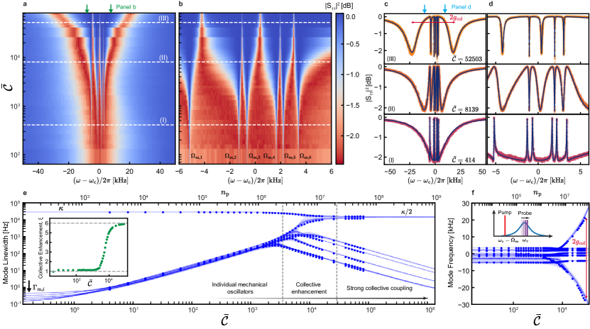
Figure 2: Emergence of dark and bright collective modes. a, Wide span and b, zoomed-in optomechanically induced transparency (OMIT) response. The bare mechanical frequencies are labeled in low cooperativity regime. Three cross sections (white lines) are shown in panels c and d. c, Three OMIT traces (circles) and fits (solid line) using the theoretical model. d, The zoomed-in OMIT traces. In a-d, we have removed the Fano interference for better visibility of the microwave response. e, Linewidths of modes using the fitted values. The dots are extracted from the experimental data and the blue line is the theoretical expectation. The blue shaded region reflects 90% percent certainty range by considering uncertainties in parameters. The inset shows the collective enhancement factor $\xi$. The first dashed line determines the region with $\xi\geq 2$. The second dashed line determines the region with $>90\%$ hybridization. f, The extracted mode frequencies and the theory prediction. In the strong coupling regime, the primary cavity and the bright collective mode hybridize and their frequencies split by twice of the collectively enhanced optomechanical coupling rate $g_{\rm col}$. Schematic of the multi-mode OMIT measurement is shown in inset. The top axis is the photon number inside the cavity ($n_{\rm p}$) and the bottom axis is the average of cooperativities ($\mathcal{\bar{C}}$).

To investigate bright and dark collective modes, we conduct an optomechanically induced transparency (OMIT) experiment [50], in which we send a coherent tone (pump) at the red sideband of the primary cavity, detuned by $\bar{\Omega}_{\rm{m}}$. We measure the reflection $S_{11}(\omega)$ around the cavity frequency using a weak probe (Fig. 2f inset). A wide span response and a zoomed-in one are plotted in Figs. 2a and b, respectively, for varying pump powers. As it is shown in Figs. 2c and d, the theoretical model can accurately predict experimental data. Using the fitting results at each pump power, we extract the linewidths and frequencies of the system modes (the system is composed of six mechanical oscillators and one microwave mode), as it is plotted in Figs. 2e and f, respectively, versus average of cooperativities $\overline{\cal C}=4\overline{g_{i}^{2}/\kappa{\Gamma_{{\rm{m}},i}}}$, where $\Gamma_{{\rm m},i}$ is the damping rate and $g_{i}$ is the optomechanical coupling rate of the $i$th mechanical oscillator. As the pump power increases, $g_{i}$ scales with the intra-cavity photon number $n_{\rm p}$ according to $g_{i}=g_{0,i}\sqrt{n_{\rm p}}$, where $g_{0,i}$ is the single-photon optomechanical coupling rate of the $i$th mechanical oscillator. In our device, $\bar{g}_{0,i}/2\pi=1.3$ Hz, which is six times smaller than that of an optomechanical system with a single mechanical oscillator, as the optomechanical coupling rates inherit the microwave mode distribution of the primary cavity (see SI and [42]).

At low powers, $\mathcal{\bar{C}}\approx\mathcal{O}(10^{1}-10^{3})$, we observe six transparency windows in the reflection spectrum, corresponding to the OMIT features of individual mechanical oscillators. By increasing the pump power, the linewidth of each mechanical oscillator increases due to its optomechanical damping rate $\Gamma_{{\rm opt},i}=4g_{i}^{2}/\kappa$. As long as $|\Omega_{{\rm{m}},i}-\Omega_{{\rm{m}},j}|\gg\Gamma_{{\rm{opt}},i},\Gamma_{{\rm{opt}},j}$, the modes remain individual mechanical oscillators, evidenced by a linear increase in all of the mechanical linewidths with respect to the pump power (Fig. 2e). As the pump power increases further, the frequency difference between independent mechanical oscillators becomes comparable to their linewidths $\Gamma_{{\rm opt},i}$. Upon meeting this criterion for all the mechanical oscillators, $\mathcal{\bar{C}}\approx\mathcal{O}(10^{3}-10^{4})$, they become indistinguishable and a transition occurs from independent oscillators to collective modes, in which the thermomechanical sidebands scattered from different individual mechanical oscillators start to interfere in the feedline, leading to either a suppression or enhancement of the optomechanical damping rates. Such interference is similar to what leads to the noise dynamics in non-reciprocal optomechanical circuits, where the interference of pathways leads to a transparency window [40]. The onset of such transition is the appearance of dark and bright collective modes, where the former are identified by their linewidths decreasing with increasing pump power. The bright collective mode, on the contrary, is identifiable by its linewidth increase compared to a single optomechanical system. To quantify such collective enhancement, we define the collective optomechanical coupling rate $g_{\rm col}=\left|{\left\langle{{{\psi}}}\mathrel{\left|{\vphantom{{\psi}{{g_{i}}}}}\right.\kern-1.2pt}{{{g_{i}}}}\right\rangle}\right|$, where $\left|{{\psi}}\right\rangle$ is the vector of the bright collective mode found through the OMIT measurement and $\left|{{g_{i}}}\right\rangle={\left({{g_{1}},...,{g_{N}}}\right)^{t}}$. It quantifies the coupling of the bright collective mode to the primary cavity and simplifies to $\sqrt{N}g$ in the ideal case. In Fig. 2e inset, we plot the collective enhancement $\xi={{{g_{{\rm{col}}}^{2}}/\overline{g_{i}^{2}}}}$, which starts from 1, signifying no collective enhancement, and approaching $N=6$, which is the maximum of enhancement. At higher powers, $\mathcal{\bar{C}}\approx\mathcal{O}(10^{4}-10^{5})$, the optomechanical damping rate of the bright collective mode becomes comparable with the linewidth of the primary cavity, and they enter the strong coupling regime, similar to the single mode case [51]. In this regime, the linewidths of the hybridized modes finally become equal, $\kappa/2$, and their frequencies split by twice of the collectively enhanced optomechanical coupling rate $2g_{\rm col}$ (Fig. 2f). At the highest power, $\mathcal{\bar{C}}=81784$, the collective enhancement is $\xi=5.91$, the frequency splitting is $\Delta\omega/2\pi=48.56$ kHz, and $\Delta\omega/2{g_{{\rm{col}}}}=0.98$.

Measuring collective mechanical modeshapes

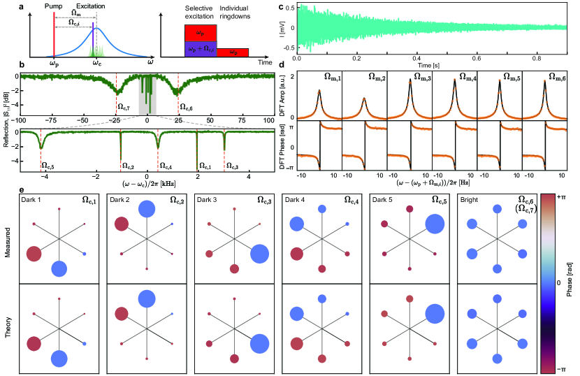
Figure 3: Modeshapes of dark and bright collective modes. a, Frequency and pulse scheme: each collective mode is selectively excited by sending an excitation signal that is blue-detuned from the pump by the frequency of the respective collective mode. Its modeshape is then measured by a weak pump that is red-detuned, allowing for the ringdown measurement of individual oscillators. b, OMIT response (wide span and zoomed-in) for the cooperativity $\mathcal{\bar{C}}=82685$. Two broad dips in the wide-span response correspond to the hybridization of the bright collective mode and the primary cavity. The narrow dips in the zoomed-in response correspond to dark collective modes. The corresponding mode frequencies are shown close to each resonance, which are sorted based on their linewidths. c, The in-phase signal $I(t)$ after exciting the bright mode, containing all the ringdowns of individual oscillators. d, Fourier transform of the complex signal $z(t)=I(t)+iQ(t)$ represented around each mechanical frequency $\Omega_{{\rm m},i}$ e, Reconstructed modeshapes of collective modes with frequencies $\Omega_{{\rm c},i}$ in the phase space of individual mechanical oscillators. Each mechanical oscillator is represented by a circle, its radius is given by the participation ratio of the mechanical oscillator to the mode, and its color shows the relative phase. The top row and the bottom row show the measured modeshape and the inferred values (from fitting to the OMIT response), respectively. The modes are sorted based on their linewidths. Modes with frequencies $\Omega_{{\rm c},6}$ and $\Omega_{{\rm c},7}$ have the same mechanical modeshape (due to the hybridization with the primary cavity), so we just plot the former.

Next, we directly measure both the amplitudes and relative phases of the bright and dark collective modes. We leverage the finite non-degeneracy of mechanical frequencies ($0.1\%$) together with quenching of the optomechanical couplings to switch between the individual and collective dynamics. This initiates the ringdown of individual mechanical oscillators at their bare frequencies. The amplitude and relative phase of the ringdowns provide us with the amplitude and relative phase of the collective modeshapes. For a given pump power, red detuned from the primary cavity by $\bar{\Omega}_{\rm m}$, we determine the bright and dark collective mode frequencies ($\Omega_{{\rm c},i}$) through an OMIT experiment, as outlined previously. The OMIT trace is shown in Fig. 3b for $\mathcal{\bar{C}}=82685$. Subsequently, we employ a time domain protocol, where a pulsed pump is sent along with a pulsed excitation signal blue-detuned from the pump by the frequency of the target collective mode $\Omega_{{\rm c},i}$ to selectively excite it (Fig. 3a). The beating between the pump and the excitation signal excites the mechanical oscillators according to their participation in the collective mode being excited. For example, by selectively exciting the bright collective mode, we expect to excite all the mechanical oscillators with the same amplitude and relative phase. After waiting for $\tau\gg 1/\Gamma_{{\rm opt},i}$, we quench the optomechanical coupling rates by turning off the excitation signal and reducing the pump power, which initiates the ringdown of the mechanical oscillators. The optomechanical damping rates after quenching satisfy $\Gamma_{{\rm{opt}},i,j}\approx 10\Gamma_{{\rm{m}},i,j}\ll|\Omega_{{\rm{m}},i}-\Omega_{{\rm{m}},j}|$, allowing us to characterize them individually at their bare frequencies while measuring them faster than their internal decay rates. The in-phase and out-of-phase quadrature ringdown signals, $I(t)$ and $Q(t)$ respectively, around the cavity frequency are then recorded (Fig. 3c). With both quadratures, the complex signal in the rotating frame of the pump can be expressed as: $z(t\geq 0)=I(t)+iQ(t)=\sum\limits_{j=1}^{N}{{A_{j}}{e^{-i({\Omega_{{\rm{m}},j}}t-{\varphi_{j}})-{\Gamma_{{\rm{m}},j}}t/2}}}$, where $\varphi_{j}$ and ${A_{j}}$ denote the relative phase and amplitude of each mechanical oscillator within the selectively excited collective mode, respectively.

We perform a Fourier transform on the complex signal to extract both the amplitude and the relative phase of the individual mechanical ringdowns (see SI). The result for the bright collective mode is presented in Fig. 3d. We can repeat the same procedure for all collective modes to extract their modeshapes. The reconstructed modeshapes (amplitude and relative phase) and the theoretical values (see SI) are depicted in Fig. 3e, demonstrating an excellent agreement between the two. Notably, in the bright collective mode, all mechanical oscillators exhibit nearly identical amplitude and relative phase. Conversely, the dark collective modes are localized on one or more oscillators.

Ground-state cooling of the bright collective mode

The high quality factors of individual mechanical oscillators (averaging $11\times 10^{6}$, average of thermal decoherence rates $\overline{{\Gamma_{{\rm{th}},i}}}\left({\equiv\overline{{\Gamma_{{\rm{m}},i}}n_{{\rm{m}},i}^{{\rm{th}}}}}\right)/2\pi=53.7\pm 3.4$ Hz, where ${n_{{\rm{m}},i}^{{\rm{th}}}}$ is the occupation of the $i$th mechanical bath) enables us to prepare the bright collective mode in its quantum ground state. We employ the sideband cooling method [14] by applying a pump red-detuned from the primary cavity by $\bar{\Omega}_{\rm m}$, along with using filter cavities at room temperature to remove the pump phase noise around the cavity frequency (see SI). The thermomechanical sideband around the cavity frequency is then detected and fitted to the model based on quantum Langevin equations together with input-output relations (see Fig. 4a and SI). As it is evident from Fig. 4d, the theoretical model accurately reproduces experimental data across different ranges of pump powers. Having all the parameters of the system, we can construct the covariance matrix of mechanical quadratures. Eigenvalues of this matrix correspond to the occupation of dark and bright collective modes (see SI). The occupation of the bright collective mode, reported in Fig. 4b, remains below one quanta for a wide range of powers, reaching a minimum of $n_{\rm m}=0.40\pm 0.02$ quanta, constrained by the heating of the primary cavity [14]. The quantum efficiency of the measurement chain utilized to derive the occupations in Fig. 4b is determined through a temperature sweep of the dilution fridge (see SI). To assess the overlap between the measured bright collective mode and the ideal one, we plot in Fig. 4c the modeshape fidelity based on the eigenvectors of the covariance matrix (see SI), which starts from 1/6, meaning the mode is localized in one of the oscillators, and approaches 1, signifying equal distribution of the amplitude across all the sites with zero relative phase.

To corroborate the occupation measurement, we conduct an optomechanical quantum sideband asymmetry experiment [52, 15, 31, 36]. In this experiment, the asymmetry in the Stokes and anti-Stokes thermomechanical sidebands is used to extract the mechanical occupation. This experiment is performed in two distinct regimes: (i)- when the pump power is sufficiently low ($\mathcal{\bar{C}}\approx\mathcal{O}(10^{2}-10^{3})$) such that the mechanical oscillators remain in their individual basis, and (ii)- when the pump power is high ($\mathcal{\bar{C}}\approx\mathcal{O}(10^{4}-10^{5})$), causing the bright collective mode to emerge and enter the strong coupling regime with the primary cavity. To measure the sidebands, we exploit the auxiliary cavity and apply a probe tuned at its center frequency (Fig. 4e). We use filter cavities at the upper and lower motional sidebands of the probe to remove the source phase noise such that quantum backaction dominates. The Stokes and anti-Stokes sidebands are proportional to $n_{\rm m}+1+2n_{\rm aux}$ and $n_{\rm m}-2n_{\rm aux}$, respectively, where $n_{\rm aux}$ represents the heating of the auxiliary cavity. In the first regime, we select the lowest frequency mechanical oscillator, which is the furthest from the others (Fig. 4g). In the second regime, the sidebands are described by the strong coupling between the primary cavity and the bright collective mode [14], evidenced by the doublet in the observed sidebands. We neglect the dark modes in the fitting model due to their negligible linewidths compared to that of the bright collective mode (Fig. 4i). By utilizing the difference between the areas of the sidebands, along with considering the heating of the auxiliary cavity caused by the strong pump (see SI), we extract the mechanical occupations. As depicted in Figs. 4f and h, the occupation extracted using sideband asymmetry closely aligns with that obtained from the temperature-sweep-calibrated quantum efficiency, thereby affirming the validity of the results in Figs. 4b. It is worth mentioning that the occupation of the mechanical oscillator in Figs. 4f is larger than those shown in Fig. 4b, primarily due to the non-negligible quantum backaction of the resonant probe on the auxiliary cavity (see SI and [31, 36]).

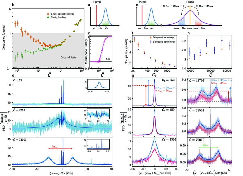
Figure 4: Ground-state cooling and quantum sideband asymmetry of the bright collective mode. a, Measurement scheme for sideband cooling of the bright collective mode. Here, no pump is present at the auxiliary cavity. b, Occupation of the bright collective mode (orange circles) and heating of the primary cavity (green circles). The gray shaded region shows the ground state. c, Fidelity between the ideal bright collective mode and the measured one versus average of cooperativities. d, Output spectrum from the cavity and fit (black line) for three different cooperativities. Insets show the zoomed-in spectra. e, Pumping scheme using the primary cavity for cooling and the auxiliary cavity for sideband asymmetry experiment. The Stokes and anti-Stokes sidebands are generated by pumping at the center frequency of the auxiliary cavity. f, Extracted occupation of the lowest frequency mechanical oscillator at low cooling powers using sideband asymmetry (blue circles) and temperature-sweep-calibrated quantum efficiency (orange circles). g, Stokes and anti-Stokes sidebands of the lowest frequency mechanical oscillator at low powers. h, Extracted occupation of the bright collective mode when it is strongly coupled to the primary cavity using sideband asymmetry and calibrated quantum efficiency. i, Stokes and anti-Stokes sidebands when the bright collective mode is strongly coupled to the microwave cavity. The unequal height of the peaks for each sideband is due to the finite detuning of the cooling pump from the optimal frequency. The anti-Stokes sideband is mirrored with respect to the center frequency.

Conclusion and outlook

In summary, we observed collective phenomena in an optomechanical system composed of a mechanical hexamer. Our investigation revealed a bright collective mode of nearly degenerate mechanical oscillators, with identical amplitudes and phases, whose coupling to the cavity increases with the number of oscillators. By further increasing the coupling, this mode enters the strong coupling regime with the cavity. Exploiting the slight non-degeneracy of oscillators, we directly measure the amplitude and phase of the collective mechanical modes. Finally, we prepare the bright collective mode in its quantum ground state and observe the quantum sideband asymmetry of its Stokes and anti-Stokes sidebands. This experiment lays the groundwork for exploring large-scale synchronization [10], investigating topological phases of sound [11], and more broadly, multi-partite phonon-phonon [16, 17] and photon-phonon [18] entanglement. Looking forward, integrating our system with superconducting qubits enables us to simulate more advanced systems, such as spin-boson models [53] with mechanical oscillators.

Data and materials availability

The code and data used to produce the plots within this paper will be available at a Zenodo open-access repository. All other data used in this study are available from the corresponding authors upon reasonable request.

Supplementary Note 1.   System parameters and variables

Table 1: System parameters

Parameter	Symbol	Value
Microwave cavity frequency (individual sites)	$\omega_{\mathrm{0}}$	$2\pi\;\times$ 5.427 GHz
Microwave inter-cavity coupling	$J$	$2\pi\;\times$ 367 MHz
Primary cavity frequency	$\omega_{\mathrm{c}}$	$2\pi\;\times$ 4.814 GHz
Primary cavity linewidth: $\kappa=\kappa_{\mathrm{ex}}+\kappa_{\mathrm{0}}$	$\kappa$	$2\pi\;\times$ 32 kHz
Primary cavity external coupling rate	$\kappa_{\mathrm{ex}}$	$2\pi\;\times$ 25 kHz
Primary cavity internal loss rate	$\kappa_{\mathrm{0}}$	$2\pi\;\times$ 7 kHz
Auxiliary cavity frequency	$\omega_{\mathrm{aux}}$	$2\pi\;\times$ 6.420 GHz
Auxiliary cavity linewidth: $\kappa_{\rm aux}=\kappa_{\mathrm{ex}}^{\rm aux}+\kappa_{\mathrm{0}}^{\rm aux}$	$\kappa_{\rm aux}$	$2\pi\;\times$ 14.7 MHz
Auxiliary cavity external coupling rate	$\kappa_{\mathrm{ex}}^{\rm aux}$	$\ 2\pi\;\times$ 11.94 MHz
Auxiliary cavity internal loss rate	$\kappa_{\mathrm{0}}^{\rm aux}$	$\ 2\pi\;\times$ 2.75 MHz
Average of mechanical frequencies	$\bar{\Omega}_{\mathrm{m}}$	$2\pi\;\times$ 1.991 MHz
Standard deviation of mechanical frequencies	$\sigma_{\Omega_{\mathrm{m}}}$	$2\pi\;\times$ 2.83 KHz
Average of mechanical bare damping rates	$\bar{\Gamma}_{\mathrm{m}}$	$2\pi\;\times$ 212 mHz
Average of mechanical quality factors	$\bar{Q}_{\mathrm{m}}$	$11\times 10^{6}$
Average of single-photon optomechanical coupling rates (coupled to the primary cavity)	$\bar{g}_{0}$	$2\pi\;\times$ 1.30 Hz

Table 2: Individual mechanical oscillator frequencies $\Omega_{{\rm m},i}$, single photon optomechanical coupling rates $g_{0,i}$, and quality factors $Q_{{\rm m},i}$.

Number $i$	$(\Omega_{{\rm m},i}-{\bar{\Omega}_{\rm m}})/2\pi$	$g_{0,i}(\equiv g_{0,i}^{\prime}/6)/2\pi$	$Q_{{\rm m},i}(\times 10^{6})$
1	-5.19 kHz	$1.35\pm 0.01$ Hz	16.84
2	-1.3 kHz	$1.34\pm 0.01$ Hz	7.84
3	-0.68 kHz	$1.42\pm 0.01$ Hz	15.87
4	+1.63 kHz	$1.25\pm 0.01$ Hz	11.80
5	+2.18 kHz	$1.25\pm 0.01$ Hz	8.26
6	+3.37 kHz	$1.25\pm 0.01$ Hz	5.56

Table 3: Variables

Variables	Symbol
Annihilation operator for primary cavity	$\hat{a}$
Annihilation operator for the $i$th mechanical oscillator	$\hat{b}_{i}$
Noise operator for primary cavity intrinsic bath	$\hat{a}_{0}^{\rm{in}}$
Noise operator for primary cavity external bath	$\hat{a}_{\rm{ex}}^{\rm{in}}$
Noise operator for the $i$th mechanical intrinsic bath	$\hat{b}_{0,i}^{\rm{in}}$
Primary cavity thermal bath occupation	$n_{\mathrm{c}}^{\mathrm{th}}$
Auxiliary cavity thermal bath occupation	$n_{\mathrm{aux}}^{\mathrm{th}}$
Primary cavity thermal occupation	$n_{\mathrm{c}}$
Auxiliary cavity thermal occupation	$n_{\mathrm{aux}}$
Mechanical thermal bath occupation ($i$th oscillator)	$n_{\mathrm{m},i}^{\mathrm{th}}$
Intra-cavity photon number induced by cooling pump	$n_{\mathrm{p}}$
Single photon Optomechanical coupling rate ($i$th oscillator, coupled to individual resonators)	$g_{0,i}^{\prime}$
Single photon Optomechanical coupling rate ($i$th oscillator, coupled to the primary cavity): $g_{0,i}\equiv g_{0,i}^{\prime}/6$	$g_{0,i}$
Optomechanical coupling rate induced by pump ($i$th oscillator, coupled to the primary cavity): $g_{i}\equiv g_{0,i}\sqrt{n_{\rm p}}$	$g_{i}$
Average optomechanical cooperativity: $\mathcal{\bar{C}}=\overline{\frac{{4g_{i}^{2}}}{{\kappa{\Gamma_{i}}}}}$	$\mathcal{\bar{C}}$
Total added noise of microwave measurement chain	$n_{\rm{add}}$
HEMT effective added noise	$n_{\rm{add}}^{\rm{H}}$
Occupation of the bright collective mode	$n_{\rm m}$
Occupation of the $i$th mechanical oscillator	$n_{{\rm m},i}$

Supplementary Note 2.   Theory

In this section we provide the theoretical framework in which we describe the system and the experimental measurement protocols.

2.1 Full microwave circuit model

A complete electrical equivalent circuit for the device reported in Fig. 1 of the main text must incorporate inductive coupling between nearest neighbors as well as stray capacitance to ground, as shown in Fig. S7. It is important to note that we disregard the stray capacitive coupling of two adjacent sites, as our experimental and numerical analysis (see Sec. 3) indicates its negligible contribution.

Figure S1: Full equivalent circuit model. The single lines correspond to coupling between different resonators, where the solid line represent nearest neighbor coupling, the dashed line is the second-nearest-neighbor coupling, and the dotted line shows the third-nearest-neighbor coupling. In the same fashion, the double line signals the coupling of individual resonators with the feedline. All coupling are dominated by the inductive part, denoted with the symbol $M_{\rm x}$. The numbers label the individual resonators.

The capacitor $\bf{C}$ and the inductor $\bf{L}$ matrices are given by

$$\bf C=\left(\begin{array}[]{cccccc}C_{\rm d}+C_{\rm s}&0&0&0&0&0\\ 0&C_{\rm d}+C_{\rm s}&0&0&0&0\\ 0&0&C_{\rm d}+C_{\rm s}&0&0&0\\ 0&0&0&C_{\rm d}+C_{\rm s}&0&0\\ 0&0&0&0&C_{\rm d}+C_{\rm s}&0\\ 0&0&0&0&0&C_{\rm d}+C_{\rm s}\\ \end{array}\right),\quad\bf L=\left(\begin{array}[]{cccccc}L&-M_{1}&-M_{2}&-M_{3}&-M_{2}&-M_{1}\\ -M_{1}&L&-M_{1}&-M_{2}&-M_{3}&-M_{2}\\ -M_{2}&-M_{1}&L&-M_{1}&-M_{2}&-M_{3}\\ -M_{3}&-M_{2}&-M_{1}&L&-M_{1}&-M_{2}\\ -M_{2}&-M_{3}&-M_{2}&-M_{1}&L&-M_{1}\\ -M_{1}&-M_{2}&-M_{3}&-M_{2}&-M_{1}&L\\ \end{array}\right),$$ (1)

where $C_{\rm d}$ is the drum capacitance and $C_{\rm s}$ is the stray capacitance of the electrodes to the ground. The same sign for all the mutual inductance terms (the off-diagonal terms in $\bf L$) is a direct consequence of the identical orientation of the spiral inductors in our design. The Lagrangian $\mathcal{L}$ of the circuit can be written as a function of node flux (voltage drop across each capacitor) $\bm{\phi}$ $=(\phi_{1},\phi_{2},\phi_{3},\phi_{4},\phi_{5},\phi_{6})$:

$$\mathcal{L}=\frac{1}{2}\bm{\dot{\phi}}^{T}\mathbf{C}\bm{\dot{\phi}}-\frac{1}{2}\bm{\phi}^{T}\mathbf{L}^{-1}\bm{\phi},$$ (2)

and the normal modes are obtained by solving the equations of motion with the ansatz $\bm{\phi}_{0}e^{i\omega t}$: $\left(\omega^{2}\mathbf{C}-\mathbf{L}^{-1}\right)\bm{\phi}_{0}=0$. The microwave mode frequencies are given by

$$\bm{\omega}=\rm{Diag}(\sqrt{\mathbf{L}^{-1}\mathbf{C}^{-1}}),$$ (3)

that can be explicitly written as

$$\bm{\omega}=\left(\begin{array}[]{c}1/\sqrt{C_{\rm tot}(L-2M_{1}-2M_{2}-M_{3})}\\[3.0pt] 1/\sqrt{C_{\rm tot}(L-M_{1}+M_{2}+M_{3})}\\[3.0pt] 1/\sqrt{C_{\rm tot}(L-M_{1}+M_{2}+M_{3})}\\[3.0pt] 1/\sqrt{C_{\rm tot}(L+M_{1}+M_{2}-M_{3})}\\[3.0pt] 1/\sqrt{C_{\rm tot}(L+M_{1}+M_{2}-M_{3})}\\[3.0pt] 1/\sqrt{C_{\rm tot}(L+2M_{1}-2M_{2}+M_{3})}\\[3.0pt] \end{array}\right),$$ (4)

where $C_{\rm tot}=C_{\rm d}+C_{\rm s}$ and the frequencies are ordered from the largest to the smallest.

From the experimentally measured mode frequencies and the numerical simulation to estimate the ratio between the stray and vacuum gap capacitance (see Sec. 6.1 for more details), we can extract the circuits parameters, which are reported in table 4.

Table 4: Circuit parameters.

Parameter	Value
$C_{\rm d}$	75.2 fF
$C_{\rm s}$	37.3 fF
$L$	7.859 nH
$M_{1}$	1.010 nH
$M_{2}$	0.125 nH
$M_{3}$	0.086 nH

It is worth mentioning that the circuit symmetry gives rise to the degeneracy of two pairs of microwave modes. Small fluctuation in circuits parameters, experimentally accounted to capacitance variation due to gap-size fluctuations, breaks such symmetry and results in non degenerate modes. However, as we see in Sec. 3.1, the modeshapes of interest (the primary and auxiliary cavities) are very robust to fabrication imperfections.

Following the derivation in [1, 2], the Hamiltonian is obtained from the Lagrangian using a Legendre transformation $\mathcal{H}=\mathbf{q}^{T}\bm{\dot{\phi}}-\mathcal{L}$, where $\mathbf{q}=(q_{1},q_{2},q_{3},q_{4},q_{5},q_{6})$ is the vector of conjugate variables $q_{i}=\partial\mathcal{L}/\partial\dot{\phi}_{i}$. In this case we obtain

$$\mathcal{H}=\frac{1}{2}\bm{q}^{T}\mathbf{C}^{-1}\bm{q}+\frac{1}{2}\bm{\phi}^{T}\mathbf{L}^{-1}\bm{\phi}.$$ (5)

By introducing the frequency of the each individual resonators approximated in the first orders in $\frac{M_{i}}{L}$,

$$\omega_{0}=\frac{1}{\sqrt{LC_{\rm tot}}}\left(1+30\frac{M_{1}}{2L}\frac{M_{2}}{2L}\frac{M_{3}}{2L}\right),$$ (6)

and by promoting $\bm{q}$ and $\bm{\phi}$ to operators, such that their commutation relation reads $\left[\hat{\phi}_{m},\hat{q}_{n}\right]=i\delta_{mn}\hbar$, we introduce the creation and annihilation operators for the single microwave resonator

$$\hat{\phi}_{m} =\phi_{\rm zpf}(\hat{a}_{m}^{\prime\dagger}+\hat{a}_{m}^{\prime})=\sqrt{\frac{\hbar}{2}\frac{1}{\omega_{0}C_{\rm tot}}}(\hat{a}_{m}^{\prime\dagger}+\hat{a}_{m}^{\prime}),$$ (7)

$$\hat{q}_{n} =iq_{\rm zpf}(\hat{a}_{n}^{\prime\dagger}-\hat{a}_{n}^{\prime})=i\sqrt{\frac{\hbar}{2}\omega_{0}C_{\rm tot}}(\hat{a}_{n}^{\prime\dagger}-\hat{a}_{n}^{\prime}).$$

From these expressions, we can introduce the nearest-neighbor coupling $J_{1}$, the second-nearest-neighbor coupling $J_{2}$, and the third-nearest-neighbor coupling $J_{3}$, as

$$J_{1} =\omega_{0}\left(\frac{M_{1}}{2L}+3\frac{M_{1}}{2L}\frac{M_{2}}{2L}+3\frac{M_{2}}{2L}\frac{M_{3}}{2L}\right),$$ (8)

$$J_{2} =\omega_{0}\left(\frac{M_{2}}{2L}+3\frac{M_{1}}{2L}\frac{M_{3}}{2L}+15\frac{M_{1}}{2L}\frac{M_{2}}{2L}\frac{M_{3}}{2L}\right),$$

$$J_{3} =\omega_{0}\left(\frac{M_{3}}{2L}+6\frac{M_{1}}{2L}\frac{M_{2}}{2L}\right),$$

which are approximated in the first order in $M_{i}/L$. With these elements, the final Hamiltonian for the microwave part reads

$$\hat{H}_{0}/\hbar=\sum_{n}^{N}\omega_{0}\hat{a}^{\prime\dagger}_{n}\hat{a}_{n}^{\prime}+J_{1}\left(\hat{a}_{n}^{\prime\dagger}\hat{a}_{n+1}^{\prime}+\hat{a}_{n}^{\prime}\hat{a}_{n+1}^{\prime\dagger}\right)+J_{2}\left(\hat{a}_{n}^{\prime\dagger}\hat{a}_{n+2}^{\prime}+\hat{a}_{n}^{\prime}\hat{a}_{n+2}^{\prime\dagger}\right)+\frac{1}{2}J_{3}\left(\hat{a}_{n}^{\prime\dagger}\hat{a}_{n+3}^{\prime}+\hat{a}_{n}^{\prime}\hat{a}_{n+3}^{\prime\dagger}\right)$$ (9)

with the convention $\hat{a}_{N+1}^{\prime}=\hat{a}_{1}^{\prime}$, $\hat{a}_{N+2}^{\prime}=\hat{a}_{2}^{\prime}$ and $\hat{a}_{N+3}^{\prime}=\hat{a}_{3}^{\prime}$. Hamiltonian (9) can be written in the matrix form as

$$\hat{H}_{0}=\hbar\bm{\hat{a}}^{\prime\dagger}\bm{H_{0}}\bm{\hat{a}}^{\prime}=\hbar\left(\begin{array}[]{cccccc}\hat{a}_{1}^{\prime\dagger}&\hat{a}_{2}^{\prime\dagger}&\hat{a}_{3}^{\prime\dagger}&\hat{a}_{4}^{\prime\dagger}&\hat{a}_{5}^{\prime\dagger}&\hat{a}_{6}^{\prime\dagger}\\ \end{array}\right)\left(\begin{array}[]{cccccc}\omega_{0}&J_{1}&J_{2}&J_{3}&J_{2}&J_{1}\\ J_{1}&\omega_{0}&J_{1}&J_{2}&J_{3}&J_{2}\\ J_{2}&J_{1}&\omega_{0}&J_{1}&J_{2}&J_{3}\\ J_{3}&J_{2}&J_{1}&\omega_{0}&J_{1}&J_{2}\\ J_{2}&J_{3}&J_{2}&J_{1}&\omega_{0}&J_{1}\\ J_{1}&J_{2}&J_{3}&J_{2}&J_{1}&\omega_{0}\\ \end{array}\right)\left(\begin{array}[]{c}\hat{a}_{1}^{\prime}\\ \hat{a}_{2}^{\prime}\\ \hat{a}_{3}^{\prime}\\ \hat{a}_{4}^{\prime}\\ \hat{a}_{5}^{\prime}\\ \hat{a}_{6}^{\prime}\\ \end{array}\right).$$ (10)

Introducing the base $\left|n\right\rangle=(\delta_{1n},\delta_{2n},\delta_{3n},\delta_{4n},\delta_{5n},\delta_{6n})^{\rm t}$, where $\delta_{ij}$ is the Kronecker delta and $\delta_{ij}=1$ if $i=j$, the Hamiltonian matrix $\bm{H_{0}}$ is diagonalized by the matrix $U$, where its elements are given by

$$U_{nm}=\frac{1}{\sqrt{6}}e^{in\frac{2\pi m}{N}},\qquad{\rm for}\quad n\in\{0,\pm 1,\pm 2,3\},\quad m\in\{1,2,3,4,5,6\},$$ (11)

resulting in the modes frequencies

$$\bm{\omega}=\left(\begin{array}[]{c}\omega_{0}+2J_{1}+2J_{2}+J_{3}\\[3.0pt] \omega_{0}+J_{1}-J_{2}-J_{3}\\[3.0pt] \omega_{0}+J_{1}-J_{2}-J_{3}\\[3.0pt] \omega_{0}-J_{1}-J_{2}+J_{3}\\[3.0pt] \omega_{0}-J_{1}-J_{2}+J_{3}\\[3.0pt] \omega_{0}-2J_{1}+2J_{2}-J_{3}\\[3.0pt] \end{array}\right),$$ (12)

and modes shape

$$\left|u_{n}\right\rangle=U_{nm}\left|m\right\rangle\qquad{\rm for}\quad n\in\{0,\overbrace{\pm 1,\pm 2}^{\text{degenerate pairs}},3\},\quad m\in\{1,2,3,4,5,6\}.$$ (13)

As shown in the main text, we experimentally measure the frequencies and the linewidths of such modes. Importantly, due to small frequency fluctuation of the microwave resonators, the degeneracy is lifted, but the frequency average of such split modes is statistically resonant with the ideal degenerate case (see Sec. 3.1 for more information). Therefore, by solving the linear system of four measured frequencies and 4 unknown parameters we extract $\omega_{0}/2\pi=5.436$ GHz, $J_{1}/2\pi=372.6$ MHz, $J_{2}/2\pi=92.2$ MHz, and $J_{3}/2\pi=61.2$ MHz.

Importantly, for our experimental implementation, the ideal mode shape for the auxiliary and primary cavities are

$$\begin{split}&\left|\text{auxiliary cavity}\right\rangle=U_{0m}\left|m\right\rangle=\frac{1}{\sqrt{6}}\left(1,1,1,1,1,1\right)^{t}\\ &\left|\text{primary cavity}\right\rangle=U_{3m}\left|m\right\rangle=\frac{1}{\sqrt{6}}\left(-1,1,-1,1,-1,1\right)^{t}.\end{split}$$ (14)

To include the coupling to the feedline, we need to take into account that all individual microwave resonators are coupled to the same microwave bath (see Fig. S1). From the quantum Langevin equations for the microwave modes $\hat{a}_{n}^{\prime}$ we have

$$\dot{\hat{a}}_{n}^{\prime}=\left(i\omega_{0}-\frac{\kappa_{n}}{2}\right){\hat{a}}_{n}^{\prime}+iJ_{1}\left(\hat{a}_{n-1}^{\prime}+\hat{a}_{n+1}^{\prime}\right)+iJ_{2}\left(\hat{a}_{n-2}^{\prime}+\hat{a}_{n+2}^{\prime}\right)+iJ_{3}\left(\hat{a}_{n+3}^{\prime}\right)+\sqrt{\kappa_{n}}\hat{a}_{\rm in}+\sum_{m\neq n}^{N}\frac{1}{2}\sqrt{\kappa_{m}\kappa_{n}}\hat{a}_{m}^{\prime},$$ (15)

where $\kappa_{i}$ represents the individual decay rates of the resonators into the waveguide. The last term in Eq. (15) produces an effective dissipative coupling between the resonators, and it arises due to the emission of the $m$th resonator to the feedline followed by the excitation of the $n$th one. Moreover, by a symmetry argument (confirmed by microwave simulations), resonators equally close to the feedline have the same decay rates, hence $\kappa_{2}=\kappa_{5}$ and $\kappa_{5}=\kappa_{6}$. We therefore introduce the non-Hermitian contribution to the Hamiltonian

$$\hat{H}_{\rm nH}/\hbar=\bm{\hat{a}}^{\dagger}\bm{H_{\rm nH}}\bm{\hat{a}},$$ (16)

where

$$\bm{H_{\rm nH}}=-\frac{i}{2}\left(\begin{array}[]{cccccc}\kappa_{1}&\sqrt{\kappa_{1}\kappa_{2}}&\sqrt{\kappa_{1}\kappa_{3}}&\sqrt{\kappa_{1}\kappa_{4}}&\sqrt{\kappa_{1}\kappa_{3}}&\sqrt{\kappa_{1}\kappa_{2}}\\ \sqrt{\kappa_{1}\kappa_{2}}&\kappa_{2}&\sqrt{\kappa_{2}\kappa_{3}}&\sqrt{\kappa_{2}\kappa_{4}}&\sqrt{\kappa_{2}\kappa_{3}}&\sqrt{\kappa_{2}^{2}}\\ \sqrt{\kappa_{1}\kappa_{3}}&\sqrt{\kappa_{2}\kappa_{3}}&\kappa_{3}&\sqrt{\kappa_{3}\kappa_{4}}&\sqrt{\kappa_{3}^{2}}&\sqrt{\kappa_{2}\kappa_{3}}\\ \sqrt{\kappa_{1}\kappa_{4}}&\sqrt{\kappa_{2}\kappa_{4}}&\sqrt{\kappa_{3}\kappa_{4}}&\kappa_{4}&\sqrt{\kappa_{3}\kappa_{4}}&\sqrt{\kappa_{2}\kappa_{4}}\\ \sqrt{\kappa_{1}\kappa_{3}}&\sqrt{\kappa_{2}\kappa_{3}}&\sqrt{\kappa_{3}^{2}}&\sqrt{\kappa_{3}\kappa_{4}}&\kappa_{3}&\sqrt{\kappa_{2}\kappa_{3}}\\ \sqrt{\kappa_{1}\kappa_{2}}&\sqrt{\kappa_{2}^{2}}&\sqrt{\kappa_{2}\kappa_{3}}&\sqrt{\kappa_{2}\kappa_{4}}&\sqrt{\kappa_{2}\kappa_{3}}&\kappa_{2}\\ \end{array}.\right)$$ (17)

Experimentally, we cannot access this matrix directly, but in the next section, we show how to infer it using the experimental data.

2.2 Microwave mode reconstruction

As mentioned above, a small disorder in the microwave frequency $\omega_{0}$ lifts the degeneracy of the degenerate mode pairs $\left|u_{\pm 1}\right\rangle$ and $\left|u_{\pm 2}\right\rangle$. Here we exploit the different values of microwave mode couplings to the feedline in order to reconstruct their modeshapes. The method consists of four main steps: 1- Introducing an additional part to the Hamiltonian wherein the frequency of the individual microwave resonators are weakly perturbed by additive Gaussian noise with zero mean; 2- Applying the original eigenvector matrix $U$ to the new Hamiltonian, resulting in a block-diagonal matrix (using the first order perturbation theory) with two $2\times 2$ blocks corresponding to the subspaces of the previously degenerate modes; 3- Introducing a new diagonalization matrix with linear combinations of $\left|u_{\pm 1}\right\rangle$ and $\left|u_{\pm 2}\right\rangle$; and 4- Diagonalizing the full non-Hermitian Hamiltonian and determining the coefficient of such linear combination that satisfy the experimental values.

Considering a small disorder on the resonators frequencies $\omega_{0}+\delta_{i}$ the system Hamiltonian reads

$${\hat{H}}/\hbar={\hat{H}_{0}}/{\hbar}+\sum_{n}^{N}\delta_{n}\hat{a}_{n}^{\prime\dagger}\hat{a}_{n}^{\prime}={\hat{H}_{0}}/{\hbar}+\hat{D}_{\delta}=\bm{\hat{a}}^{\prime\dagger}\left(\bm{H_{0}+D}\right)\bm{\hat{a}}^{\prime},$$ (18)

where the assumption $\delta_{i}/\omega_{0}\ll 1$ is justified by the small splitting of the microwave modes $\left|u_{\pm 1}\right\rangle$ and $\left|u_{\pm 2}\right\rangle$ (see Sec. 3.1 for more information). Considering a Gaussian frequency fluctuation

$$\begin{split}&\left\langle u_{n}\right|\bm{D}\left|u_{n}\right\rangle=\frac{1}{6}\sum_{n}^{6}\delta_{n}=0,\\ &\left\langle u_{n}\right|\bm{D}\left|u_{m}\right\rangle\ll\bm{\omega}_{n}-\bm{\omega}_{m}\qquad\text{for}\quad|n-m|>1,\\ &\left\langle u_{1}\right|\bm{D}\left|u_{-1}\right\rangle=\frac{1}{6}\sum_{n}^{6}\delta_{n}e^{-in\pi/3}=re^{i\phi},\\ &\left\langle u_{2}\right|\bm{D}\left|u_{-2}\right\rangle=\frac{1}{6}\sum_{n}^{6}\delta_{n}e^{-2in\pi/3}=r^{\prime}e^{i\phi^{\prime}},\end{split}$$ (19)

the full system diagonalization can be done by simply diagonalizing the two diagonal blocks related to the ideally degenerate modes. In matrix form we have

$$U^{t}\left(\bm{H_{0}+D}\right)U\approx\left(\begin{array}[]{cccccc}\omega_{\rm c}&\cdot&\cdot&\cdot&\cdot&\cdot\\ \cdot&\omega_{2}&re^{i\phi}&\cdot&\cdot&\cdot\\ \cdot&re^{-i\phi}&\omega_{2}&\cdot&\cdot&\cdot\\ \cdot&\cdot&\cdot&\omega_{4}&r^{\prime}e^{i\phi^{\prime}}&\cdot\\ \cdot&\cdot&\cdot&r^{\prime}e^{-i\phi^{\prime}}&\omega_{4}&\cdot\\ \cdot&\cdot&\cdot&\cdot&\cdot&\omega_{\rm aux}\\ \end{array}\right),$$ (20)

where dots are the higher order perturbation terms.

The unperturbed degenerate modes now split by $2r$ and $2r^{\prime}$ respectively. Such splitting can be readily measured by single tone spectroscopy. By diagonalizing each block, the new non-degenerate eigenstates of the system are

$$\begin{split}&\left|u_{1,\rm nd}\right\rangle=\frac{1}{\sqrt{2}}\left(\left|u_{1}\right\rangle+e^{-i\phi}\left|u_{-1}\right\rangle\right)\\ &\left|u_{-1,\rm nd}\right\rangle=\frac{1}{\sqrt{2}}\left(\left|u_{1}\right\rangle-e^{-i\phi}\left|u_{-1}\right\rangle\right)\\ &\left|u_{2,\rm nd}\right\rangle=\frac{1}{\sqrt{2}}\left(\left|u_{2}\right\rangle+e^{-i\phi^{\prime}}\left|u_{-2}\right\rangle\right)\\ &\left|u_{-2,\rm nd}\right\rangle=\frac{1}{\sqrt{2}}\left(\left|u_{2}\right\rangle-e^{-i\phi^{\prime}}\left|u_{-2}\right\rangle\right).\end{split}$$ (21)

The goal is now to find the parameters $\phi$ and $\phi^{\prime}$. For this, we apply the new diagonalization operator $U_{\rm nd}$ to the non-Hermitian component of the Hamiltonian $\bm{H_{\rm nH}}$, giving rise to a system of 6 unknowns ($\phi,\phi^{\prime},\kappa_{1},\kappa_{2},\kappa_{3},\kappa_{4}$) in 6 experimentally measured modes couplings. However, such system does not have an analytical solutions and we calculate its solutions by minimizing the cost function

$$\sum_{n}^{N}\left(\text{Imag}\left[U_{\rm nd}^{t}\bm{H_{\rm nH}}U_{\rm nd}\right]_{nn}-\kappa_{n}^{\rm exp}\right)^{2}.$$ (22)

The resulting parameters $\phi$ and $\phi^{\prime}$ are used to reconstruct the mode shape in Fig. 1 of the main text. The extracted coupling rates of each site to the feedline are found to be $\kappa_{1}/2\pi=4.45$ MHz, $\kappa_{2}/2\pi=2.24$ MHz, $\kappa_{3}/2\pi=1.34$ MHz and $\kappa_{4}/2\pi=1.09$ MHz.

2.3 Linearized optomechanical Hamiltonian

Considering the mechanical oscillators and their optomechanical interaction with the microwave resonators, the full optomechanical Hamiltonian reads

$$\hat{H}/\hbar=\bm{\hat{a}}^{\prime\dagger}\bm{H_{0}}\bm{\hat{a}}^{\prime}+\sum_{i}\Omega_{{\rm m},i}\hat{b}_{i}^{\dagger}\hat{b}_{i}+\sum_{i}g_{0,i}^{\prime}\hat{a}_{i}^{\prime\dagger}\hat{a}_{i}^{\prime}(\hat{b}_{i}^{\dagger}+\hat{b}_{i}),$$ (23)

where $\hat{b}_{i}$ represents the annihilation operator for the mechanical oscillators, and $g_{0,i}^{\prime}$ represents the single-photon optomechanical coupling rate. The microwave resonators can now be diagonalized in their basis by using the matrix $U$ in Sec. 2.1. Diagonal microwave modes $\hat{a}_{i}$ are related to the individual microwave resonators $\hat{a}_{i}^{\prime}$ as $\hat{a}_{i}=\sum_{j}U_{ij}\hat{a}^{\prime}_{j}$. The Hamiltonian in the diagonalized basis is then rewritten as

$$\hat{H}/\hbar =\sum_{i}\omega_{i}\hat{a}_{i}^{\dagger}\hat{a}_{i}+\sum_{i}\Omega_{{\rm m},i}\hat{b}_{i}^{\dagger}\hat{b}_{i}+\sum_{i}g_{0,i}^{\prime}\left(\sum_{j}U_{ji}\hat{a}^{\dagger}_{j}\right)\left(\sum_{k}U^{*}_{ki}\hat{a}_{k}\right)(\hat{b}_{i}^{\dagger}+\hat{b}_{i})$$ (24)

$$=\sum_{i}\omega_{i}\hat{a}_{i}^{\dagger}\hat{a}_{i}+\sum_{i}\Omega_{{\rm m},i}\hat{b}_{i}^{\dagger}\hat{b}_{i}+\sum_{i,j}g_{0,i}^{\prime}\left|U_{ji}\right|^{2}\hat{a}^{\dagger}_{j}\hat{a}_{j}(\hat{b}_{i}^{\dagger}+\hat{b}_{i}),$$

where $\omega_{i}$s are the microwave eigenfrequencies (12). Here we have assumed the rotating wave approximation and ignored the terms $a_{i}^{\dagger}a_{j}$ when $i\neq j$, which is valid as $|\omega_{i}-\omega_{j}|\gg g_{0,i}^{\prime}$. The collective optomechanical coupling of the $j$th microwave mode to the $i$th mechanical oscillator is $g_{0,i}^{\prime}\left|U_{ji}\right|^{2}$. In particular, for the primary and auxiliary cavities, this yields to $g_{0,i}=g_{0,i}^{\prime}/6$ for each mechanical oscillator.

From now on, we restrict the Hamiltonian (24) to the primary cavity with frequency $\omega_{\rm c}$. By considering a strong pump with frequency $\omega_{\rm p}$ red-detuned from the cavity by $\Delta=\omega_{\rm c}-\omega_{\rm p}$, the Hamiltonian simplifies to the the beam-splitter interaction (in the rotating frame of the pump):

$$\hat{H}/\hbar=\Delta\hat{a}^{\dagger}\hat{a}+\sum_{i}\Omega_{{\rm m},i}\hat{b}_{i}^{\dagger}\hat{b}_{i}+\sum_{i}{{g_{i}}\left({\hat{a}\hat{b}_{i}^{\dagger}+{{\hat{a}}^{\dagger}}{{\hat{b}}_{i}}}\right)}.$$ (25)

where $g_{i}=g_{0,i}\sqrt{n_{\rm p}}$, $n_{\rm p}$ is the number of photons inside the cavity due to the strong pump, and $\hat{a}$ is the annihilation operator of the primary cavity (we remove the subscript 3 for simplicity).

2.4 Degenerate mechanical oscillators

In this section, we show how to diagonalize the basis of degenerate mechanical oscillators. We consider the case where all the mechanical oscillators are degenerate (${\Omega_{{\rm m},i}}={\Omega_{\rm m}}\;\;\forall i\in\left\{{1,...,N}\right\}$) with the same optomechanical coupling rates (${g_{i}}=g\;\;\forall i\in\left\{{1,...,N}\right\}$). The Hamiltonian in Eq. (25) then reads:

$$\hat{H}/\hbar=\Delta{{\hat{a}}^{\dagger}}\hat{a}+{\Omega_{\rm m}}\sum\limits_{i}{\hat{b}_{i}^{\dagger}{{\hat{b}}_{i}}}+g_{i}\left({\hat{a}\sum\limits_{i}{\hat{b}_{i}^{\dagger}}+{{\hat{a}}^{\dagger}}\sum\limits_{i}{{{\hat{b}}_{i}}}}\right).$$ (26)

As it can be seen from this Hamiltonian, the cavity is now coupled to a mechanical collective mode, where all of the individual mechanics have equal amplitude and phase. This can be better seen by considering the mechanical oscillators in their own basis:

$$\Omega_{\rm m}\sum\limits_{i}{\hat{b}_{i}^{\dagger}{{\hat{b}}_{i}}}=\Omega_{\rm m}\left({\hat{b}_{1}^{\dagger}\;\;\hat{b}_{2}^{\dagger}\;\;\cdots\;\;\hat{b}_{N}^{\dagger}}\right){{\bf{I}}_{N\times N}}\left({\begin{array}[]{*{20}{c}}{{{\hat{b}}_{1}}}\\ {{{\hat{b}}_{2}}}\\ \vdots\\ {{{\hat{b}}_{N}}}\end{array}}\right),$$ (27)

where ${\bf I}$ is an identity matrix. As it is a scalar matrix, there is a freedom to choose the basis. This can be done with any unitary matrix $\bf{U}$ where $\bf{U}^{\dagger}\bf{U}=\bf{I}$. We choose the first row of matrix $\bf{U}$ (one of the eigenvectors) to be

$${{\bf{U}}_{(1,i)}}=\frac{1}{{\sqrt{N}}}\left({1\;\;1\;\;\cdots\;\;1}\right)^{t}$$ (28)

which is divided by $\sqrt{N}$ for normalization. The other rows of the matrix should be orthogonal to this row, meaning

$$\sum\limits_{j=1}^{N}{{{\bf{U}}_{(i\neq 1,j)}}}=0.$$ (29)

We now rewrite the Hamiltonian in the new basis:

$$\hat{H}/\hbar=\Delta{{\hat{a}}^{\dagger}}\hat{a}+\Omega\sum\limits_{i=1}^{N}{\hat{\beta}_{i}^{\dagger}{{\hat{\beta}}_{i}}}+g\sqrt{N}\left({\hat{a}\hat{\beta}_{1}^{\dagger}+{{\hat{a}}^{\dagger}}{{\hat{\beta}}_{1}}}\right),$$ (30)

where

$$\left({\begin{array}[]{*{20}{c}}{{{\hat{\beta}}_{1}}}\\ {{{\hat{\beta}}_{2}}}\\ \vdots\\ {{{\hat{\beta}}_{N}}}\end{array}}\right)={\bf{U}}\left({\begin{array}[]{*{20}{c}}{{{\hat{b}}_{1}}}\\ {{{\hat{b}}_{2}}}\\ \vdots\\ {{{\hat{b}}_{N}}}\end{array}}\right),$$ (31)

$${{\hat{\beta}}_{1}}=\frac{1}{{\sqrt{N}}}\sum\limits_{i=1}^{N}{{{\hat{b}}_{i}}}.$$

Now, it can be clearly seen that the microwave mode is only coupled to $\beta_{1}$, which will be referred as the bright collective mode, wherein all individual mechanical oscillators have the same amplitude and relative phase. The other collective modes are decoupled from the cavity, which is why we name them dark collective modes. In addition, we see an $\sqrt{N}$ enhancement in the coupling of the bright collective mode to the cavity.

The optomechanical damping rate of the bright collective mode induced by the pump is given by [3]:

$$\Gamma_{\rm{opt}} =\frac{4(g\sqrt{N})^{2}}{\kappa}=N\frac{4g^{2}}{\kappa}$$ (32)

$$=N\Gamma_{{\rm opt},i},$$

where $\Gamma_{{\rm opt},i}$ is the optomechanical damping rate of an individual mechanical oscillator. The linewidth of the bright collective mode is then increased by a factor of $N$. It should be noted that, here, $\Gamma_{{\rm{opt}},i}$ is the optomechanical damping rate of one of the $N$ mechanical oscillators coupled to the primary cavity. In Sec. 2.3, it is shown that by coupling to the primary cavity, the optomechanical coupling rate of each of the mechanical oscillators reduces by a factor of $N$ compared to a single-mode optomechanical system.

2.5 Multimode optomechanically induced transparency (OMIT)

In this section, we provide the theoretical details of the observed multi-mode OMIT response. We consider a pump with frequency $\omega_{\rm p}$ red-detuned by the average of the bare mechanical frequencies ${\bar{\Omega}_{\rm m}}$ from the primary cavity with frequency $\omega_{\rm c}$ and a weak probe around its center frequency (Fig. 2d inset of the main text). The linearized Hamiltonian in the rotating frame of the pump is given by Eq. (25).

The quantum Langevin equations, in the presence of a weak probe $\hat{s}_{\rm{in}}(t)$ and quantum noise, can be written as:

$$\frac{d}{{dt}}{\bf{\hat{b}}} ={\bf{M}}{\bf{\hat{b}}}+{{{\bf{\hat{b}}}_{{\rm{in}}}}},$$ (33)

$${\bf{\hat{b}}} =\left({\begin{array}[]{*{20}{c}}{\hat{a}(t)}\\ {{{\hat{b}}_{1}}(t)}\\ \vdots\\ {{{\hat{b}}_{N}}(t)}\end{array}}\right),$$

$${\bf{M}} =\left({\begin{array}[]{*{20}{c}}{-i\Delta-\kappa/2}&{-i{g_{1}}}&\cdots&{-i{g_{N}}}\\ {-i{g_{1}}}&{-i{\Omega_{{\rm m},1}}-{\Gamma_{{\rm m},1}}/2}&0&0\\ \vdots&0&\ddots&0\\ {-i{g_{N}}}&0&0&{-i{\Omega_{{\rm m},N}}-{\Gamma_{{\rm m},N}}/2}\end{array}}\right),$$

$${{{\bf{\hat{b}}}_{{\rm{in}}}}} =\left({\begin{array}[]{*{20}{c}}{\sqrt{{\kappa_{{\rm{ex}}}}}\hat{s}_{\rm{in}}(t)+\sqrt{{\kappa_{{\rm{ex}}}}}{{\hat{a}}_{{\rm{ex}}}}(t)+\sqrt{{\kappa_{\rm{0}}}}{{\hat{a}}_{\rm{0}}}(t)}\\ {\sqrt{{\Gamma_{{\rm m},1}}}\hat{b}_{0,1}^{{\rm{in}}}(t)}\\ \vdots\\ {\sqrt{{\Gamma_{{\rm m},N}}}\hat{b}_{0,N}^{{\rm{in}}}(t)}\end{array}}\right).$$

Here, $\hat{b}_{0,i}^{{\rm{in}}}(t)$ is the noise operator for the internal loss of the $i$th mechanical oscillator, ${{\hat{a}}_{{\rm{0}}}}(t)$ is the noise operator for the internal loss of the primary cavity, and ${{\hat{a}}_{{\rm{ex}}}}(t)$ is the noise operator for the external field. These operators satisfy the following relations:

$$\left\langle{\hat{a}_{{\rm{ex}}}^{\dagger}(t){{\hat{a}}_{{\rm{ex}}}}(t^{\prime})}\right\rangle=0,$$ (34)

$$\left\langle{\hat{a}_{{\rm{ex}}}(t){{\hat{a}}_{{\rm{ex}}}}^{\dagger}(t^{\prime})}\right\rangle=\delta(t-t^{\prime}),$$

$$\left\langle{\hat{a}_{\rm{0}}^{\dagger}(t){{\hat{a}}_{\rm{0}}}(t^{\prime})}\right\rangle=n_{\rm{c}}^{{\rm{th}}}\delta(t-t^{\prime}),$$

$$\left\langle{\hat{b}_{0,i}^{{\rm{in}}{\dagger}}(t)\hat{b}_{0,i}^{{\rm{in}}}(t^{\prime})}\right\rangle=n_{\rm{m,i}}^{{\rm{th}}}\delta(t-t^{\prime}),$$

$$\left\langle{\hat{b}_{0,i}^{{\rm{in}}{\dagger}}(t)\hat{b}_{0,j\neq i}^{{\rm{in}}}(t^{\prime})}\right\rangle=\left\langle{\hat{b}_{0,i}^{{\rm{in}}}(t)\hat{b}_{0,j\neq i}^{{\rm{in}}\dagger}(t^{\prime})}\right\rangle=0.$$

Here, we have assumed zero temperature for the incident microwave field and finite temperature for the internal microwave and mechanical baths with $n_{\rm{c}}^{\rm{th}}$ and $n_{\rm{m},i}^{\rm{th}}$ occupations, respectively.

The solution to Eq. (33) is found by taking a Fourier transform, leading to:

$$\left({\begin{array}[]{*{20}{c}}{-i(\omega-\Delta)+\kappa/2}&{i{g_{1}}}&\cdots&{i{g_{N}}}\\ {i{g_{1}}}&{-i(\omega-{\Omega_{{\rm m},1}})+{\Gamma_{{\rm m},1}}/2}&0&0\\ \vdots&0&\ddots&0\\ {i{g_{N}}}&0&0&{-i(\omega-{\Omega_{{\rm m},N}})+{\Gamma_{{\rm m},N}}/2}\end{array}}\right)\left({\begin{array}[]{*{20}{c}}{\hat{a}(\omega)}\\ {{{\hat{b}}_{1}}(\omega)}\\ \vdots\\ {{{\hat{b}}_{N}}(\omega)}\end{array}}\right)=$$ (35)

$$\left({\begin{array}[]{*{20}{c}}{\sqrt{{\kappa_{{\rm{ex}}}}}\hat{s}_{\rm{in}}(\omega)+\sqrt{{\kappa_{{\rm{ex}}}}}{{\hat{a}}_{{\rm{ex}}}}(\omega)+\sqrt{{\kappa_{\rm{0}}}}{{\hat{a}}_{\rm{0}}}(\omega)}\\ {\sqrt{{\Gamma_{{\rm m},1}}}\hat{b}_{0,1}^{{\rm{in}}}(\omega)}\\ \vdots\\ {\sqrt{{\Gamma_{{\rm m},N}}}\hat{b}_{0,N}^{{\rm{in}}}(\omega)}\end{array}}\right),$$

where the following convention is used for the Fourier transform:

$${\cal F}\{f(t)\} =F(\omega)=\frac{1}{{\sqrt{2\pi}}}\int_{-\infty}^{+\infty}{f(t){e^{+i\omega t}}dt}$$ (36)

$${{\cal F}^{-1}}\{F(\omega)\} =f(t)=\frac{1}{{\sqrt{2\pi}}}\int_{-\infty}^{+\infty}{F(\omega){e^{-i\omega t}}d\omega}.$$

By inverting this matrix, we can find the solution of $\hat{a}$ and $\hat{b}_{1,...,N}$. To find the linear response of the system, we ignore the quantum noise and consider only the probe field, $\hat{s}_{\rm{in}}(t)$. In this case, using input-output relation, the output field, and consequently the reflection frequency response $S_{11}(\omega)$, will be given by:

$$\hat{s}_{\rm{out}}(\omega)=\hat{s}_{\rm{in}}(\omega)-\sqrt{\kappa_{\rm{ex}}}\hat{a}(\omega),$$ (37)

and

$$S_{11}(\omega) \equiv\frac{{\left\langle{{{\hat{s}}_{{\rm{out}}}}(\omega)}\right\rangle}}{{\left\langle{{{\hat{s}}_{{\rm{in}}}}(\omega)}\right\rangle}}$$ (38)

$$=1-\frac{{{\kappa_{{\rm{ex}}}}}}{{\sum\limits_{i=1}^{N}{{\chi_{\rm{m},i}(\omega)}g_{i}^{2}}+1/{\chi_{\rm{c}}(\omega)}}},$$

where $\chi_{\rm{m},i}(\omega)^{-1}=-i(\omega-\Omega_{{\rm m},i})+\Gamma_{{\rm m},i}/2$ and $\chi_{\rm{c}}(\omega)^{-1}=-i(\omega-\Delta)+\kappa/2$ are the bare mechanical and microwave susceptibilities, respectively. Equation (38) can be considered as the generalized OMIT response in the presence of $N$ mechanical oscillators. For $N=1$, we recover the well-known OMIT response [4].

2.6 Incoherent response

In this part, we derive the output spectrum in the presence of a red detuned pump and absence of any resonant probe. Equation (35) is then rewritten in the following form:

$$\left({\begin{array}[]{*{20}{c}}{\hat{a}(\omega)}\\ {{{\hat{b}}_{1}}(\omega)}\\ \vdots\\ {{{\hat{b}}_{N}}(\omega)}\end{array}}\right)=\left({\begin{array}[]{*{20}{c}}{{A_{0}}(\omega)}&{{A_{1}}(\omega)}&\cdots&{{A_{N}}(\omega)}\\ {{B_{1,0}}(\omega)}&{{B_{1,1}}(\omega)}&\cdots&{{B_{1,N}}(\omega)}\\ \vdots&\vdots&\vdots&\vdots\\ {{B_{N,0}}(\omega)}&{{B_{N,1}}(\omega)}&\cdots&{{B_{N,N}}(\omega)}\end{array}}\right)\left({\begin{array}[]{*{20}{c}}{\sqrt{{\kappa_{{\rm{ex}}}}}{{\hat{a}}_{{\rm{ex}}}}(\omega)+\sqrt{{\kappa_{\rm{0}}}}{{\hat{a}}_{\rm{0}}}(\omega)}\\ {\sqrt{{\Gamma_{{\rm m},1}}}\hat{b}_{0,1}^{{\rm{in}}}(\omega)}\\ \vdots\\ {\sqrt{{\Gamma_{{\rm m},N}}}\hat{b}_{0,N}^{{\rm{in}}}(\omega)}\end{array}}\right),$$ (39)

where

$${A_{p}}(\omega)=\frac{{-i{g_{p}}{\chi_{p}}+(1+i{g_{p}}{\chi_{p}}){\delta_{p,0}}}}{{D(\omega)}},\;\;p\in\{0,...,N\}$$ (40)

$${B_{k,p}}(\omega)=\frac{{-i{g_{k}}{\chi_{k}}}}{{D(\omega)}}{\delta_{p,0}}+\left({{\chi_{k}}-\frac{{{g_{k}}^{2}{\chi_{k}}^{2}}}{{D(\omega)}}}\right){\delta_{k,p}}+\frac{{-{g_{k}}{g_{p}}{\chi_{k}}{\chi_{p}}}}{{D(\omega)}}(1-{\delta_{k,p}})(1-{\delta_{p,0}}),\;\;k\in\{1,...,N\},\;\;p\in\{0,...,N\}$$

$${\chi_{p}}={\chi_{\rm{c}}}(\omega){\delta_{p,0}}+{\chi_{{\rm{m}},p}}(\omega)(1-{\delta_{p,0}}),\;\;p\in\{0,...,N\}$$

$$D(\omega)=\sum\limits_{i=1}^{N}{{\chi_{{\rm{m}},i}}(\omega)g_{i}^{2}}+\chi_{\rm{c}}^{-1}(\omega).$$

Here, $\delta_{i,j}$ is Kronecker delta and $\delta_{i,j}=1$ if $i=j$ and 0 if $i\neq j$. By using Eq. (39), we find the output spectra from the cavity, the occupation of the individual mechanical oscillators, and the occupation of the collective mode.

2.6.1 Microwave output spectrum

The output field from the cavity is found using input-output relation, by considering an input vacuum microwave field to the cavity $\hat{a}_{\rm{ex}}(\omega)$:

$${{\hat{a}}_{{\rm{out}}}}(\omega) ={{\hat{a}}_{{\rm{ex}}}}(\omega)-\sqrt{{\kappa_{{\rm{ex}}}}}\hat{a}(\omega)$$ (41)

$$=\left({1-{\kappa_{{\rm{ex}}}}{A_{0}}(\omega)}\right){{\hat{a}}_{{\rm{ex}}}}(\omega)+\sqrt{{\kappa_{{\rm{ex}}}}{\kappa_{\rm{0}}}}{A_{0}}(\omega){{\hat{a}}_{\rm{0}}}(\omega)+\sum\limits_{i=1}^{N}{\sqrt{{\kappa_{{\rm{ex}}}}{\Gamma_{{\rm m},i}}}{A_{i}}(\omega)\hat{b}_{0,i}^{{\rm{in}}}(\omega)}.$$

Using the noise correlators given in Eq. (34), we find the the symmetrized output spectrum:

$${{\bar{S}}}(\omega) =\frac{1}{2}\int_{-\infty}^{+\infty}{\left\langle{{{\hat{a}}_{\rm{out}}^{\dagger}}(\omega^{\prime}){\hat{a}}_{\rm{out}}(\omega)+{\hat{a}}_{\rm{out}}(\omega^{\prime}){{\hat{a}}_{\rm{out}}^{\dagger}}(\omega)}\right\rangle d\omega^{\prime}}$$ (42)

$$=\frac{1}{2}{\left|{1-{\kappa_{{\rm{ex}}}}{A_{0}}(\omega)}\right|^{2}}+\left({n_{\rm{c}}^{{\rm{th}}}+\frac{1}{2}}\right){\kappa_{{\rm{ex}}}}{\kappa_{\rm{0}}}{\left|{{A_{0}}(\omega)}\right|^{2}}+\sum\limits_{i=1}^{N}{\left({n_{{\rm{m,}}i}^{{\rm{th}}}+\frac{1}{2}}\right){\kappa_{{\rm{ex}}}}{\Gamma_{{\rm m},i}}{{\left|{{A_{i}}(\omega)}\right|}^{2}}}.$$

This equation can be further simplified by writing the first term as follows:

$${\left|{1-{\kappa_{{\rm{ex}}}}{A_{0}}(\omega)}\right|^{2}} =1+\kappa_{{\rm{ex}}}^{2}{\left|{{A_{0}}(\omega)}\right|^{2}}-2{\kappa_{{\rm{ex}}}}\Re\left\{{{A_{0}}(\omega)}\right\}$$ (43)

$$=1+\kappa_{{\rm{ex}}}^{2}{\left|{{A_{0}}(\omega)}\right|^{2}}-2{\kappa_{{\rm{ex}}}}\frac{1}{{{{\left|{D(\omega)}\right|}^{2}}}}\Re\left\{{{D^{*}}(\omega)}\right\}$$

$$=1+\kappa_{{\rm{ex}}}^{2}{\left|{{A_{0}}(\omega)}\right|^{2}}-2{\kappa_{{\rm{ex}}}}\frac{1}{{{{\left|{D(\omega)}\right|}^{2}}}}\left({\frac{\kappa}{2}+\Re\left\{{\sum\limits_{i=1}^{N}{{\chi_{{\rm{m}},i}}(\omega)g_{i}^{2}}}\right\}}\right)$$

$$=1+\kappa_{{\rm{ex}}}^{2}{\left|{{A_{0}}(\omega)}\right|^{2}}-2{\kappa_{{\rm{ex}}}}\frac{1}{{{{\left|{D(\omega)}\right|}^{2}}}}\left({\frac{\kappa}{2}+\sum\limits_{i=1}^{N}{{{\left|{{\chi_{{\rm{m}},i}}(\omega)}\right|}^{2}}g_{i}^{2}}\Re\left\{{1/{\chi_{{\rm{m}},i}}(\omega)}\right\}}\right)$$

$$=1+\kappa_{{\rm{ex}}}^{2}{\left|{{A_{0}}(\omega)}\right|^{2}}-2{\kappa_{{\rm{ex}}}}\frac{1}{{{{\left|{D(\omega)}\right|}^{2}}}}\left({\frac{\kappa}{2}+\sum\limits_{i=1}^{N}{{{\left|{{\chi_{{\rm{m}},i}}(\omega)}\right|}^{2}}g_{i}^{2}}\frac{{{\Gamma_{{\rm m},i}}}}{2}}\right),$$

where $\Re$ stands for the real part. We now pair all the 1/2 contributions in Eq. (42) as:

$$\frac{1}{2}\left({{{\left|{1-{\kappa_{{\rm{ex}}}}{A_{0}}(\omega)}\right|}^{2}}+{\kappa_{{\rm{ex}}}}{\kappa_{\rm{0}}}{{\left|{{A_{0}}(\omega)}\right|}^{2}}+\sum\limits_{i=1}^{N}{{\kappa_{{\rm{ex}}}}{\Gamma_{{\rm m},i}}{{\left|{{A_{i}}(\omega)}\right|}^{2}}}}\right)$$ (44)

$$=\frac{1}{2}\left({1+\kappa_{{\rm{ex}}}^{2}{{\left|{{A_{0}}(\omega)}\right|}^{2}}-{\kappa_{{\rm{ex}}}}\frac{1}{{{{\left|{D(\omega)}\right|}^{2}}}}\left({\kappa+\sum\limits_{i=1}^{N}{{{\left|{{\chi_{{\rm{m}},i}}(\omega)}\right|}^{2}}g_{i}^{2}}{\Gamma_{{\rm m},i}}}\right)+{\kappa_{{\rm{ex}}}}{\kappa_{\rm{0}}}{{\left|{{A_{0}}(\omega)}\right|}^{2}}+\sum\limits_{i=1}^{N}{{\kappa_{{\rm{ex}}}}{\Gamma_{{\rm m},i}}{{\left|{{A_{i}}(\omega)}\right|}^{2}}}}\right)$$

$$=\frac{1}{2}\left({1+{\kappa_{{\rm{ex}}}}\kappa{{\left|{{A_{0}}(\omega)}\right|}^{2}}-{\kappa_{{\rm{ex}}}}\frac{1}{{{{\left|{D(\omega)}\right|}^{2}}}}\left({\kappa+\sum\limits_{i=1}^{N}{{{\left|{{\chi_{{\rm{m}},i}}(\omega)}\right|}^{2}}g_{i}^{2}}{\Gamma_{{\rm m},i}}}\right)+\sum\limits_{i=1}^{N}{{\kappa_{{\rm{ex}}}}{\Gamma_{{\rm m},i}}{{\left|{{A_{i}}(\omega)}\right|}^{2}}}}\right)$$

$$=\frac{1}{2}\left({1+{\kappa_{{\rm{ex}}}}\kappa\frac{1}{{{{\left|{D(\omega)}\right|}^{2}}}}-{\kappa_{{\rm{ex}}}}\frac{1}{{{{\left|{D(\omega)}\right|}^{2}}}}\left({\kappa+\sum\limits_{i=1}^{N}{{{\left|{{\chi_{{\rm{m}},i}}(\omega)}\right|}^{2}}g_{i}^{2}}{\Gamma_{{\rm m},i}}}\right)+\sum\limits_{i=1}^{N}{{\kappa_{{\rm{ex}}}}{\Gamma_{{\rm m},i}}\frac{{{g_{i}}^{2}{{\left|{{\chi_{{\rm{m}},i}}}\right|}^{2}}}}{{{{\left|{D(\omega)}\right|}^{2}}}}}}\right)$$

$$=\frac{1}{2},$$

where we used the explicit forms introduced in Eq. (40). The simplified spectrum then reads:

$$\bar{S}(\omega)=\frac{1}{2}+\frac{{{\kappa_{{\rm{ex}}}}{\kappa_{\rm{0}}}n_{\rm{c}}^{{\rm{th}}}}}{{{{\left|{\sum\limits_{i=1}^{N}{{\chi_{{\rm{m}},i}}(\omega)g_{i}^{2}}+\chi_{\rm{c}}^{-1}(\omega)}\right|}^{2}}}}+\frac{{\sum\limits_{i=1}^{N}{{\kappa_{{\rm{ex}}}}{\Gamma_{{\rm m},i}}{g_{i}}^{2}{{\left|{{\chi_{{\rm{m}},i}}}\right|}^{2}}n_{{\rm{m,}}i}^{{\rm{th}}}}}}{{{{\left|{\sum\limits_{i=1}^{N}{{\chi_{{\rm{m}},i}}(\omega)g_{i}^{2}}+\chi_{\rm{c}}^{-1}(\omega)}\right|}^{2}}}}.$$ (45)

In this equation, the first term is the vacuum noise, the second term is the contribution of the cavity heating, and the last term is the contribution of each of the mechanical oscillators.

2.6.2 Individual and cross mechanical spectrums

Although we do not have direct access to each individual/physical mechanical oscillator (with $\hat{b}_{i}$ operator), we can find their occupations and their cross-correlations, respectively, using Eq. (39):

$${S_{\hat{b}_{i}^{\dagger}{{\hat{b}}_{i}}}}(\omega)= \int_{-\infty}^{+\infty}{\left\langle{\hat{b}_{i}^{\dagger}(\omega^{\prime}){{\hat{b}}_{i}}(\omega)}\right\rangle d\omega^{\prime}}$$ (46a)

$$= \frac{{g_{i}^{2}{{\left|{{\chi_{{\rm{m}},i}}}\right|}^{2}}}}{{|D(\omega){|^{2}}}}{\kappa_{0}}n_{\rm{c}}^{{\rm{th}}}+{\left|{{\chi_{{\rm{m}},i}}-\frac{{{g_{i}}^{2}{\chi_{{\rm{m}},i}}^{2}}}{{D(\omega)}}}\right|^{2}}{\Gamma_{{\rm m},i}}n_{{\rm{m}},i}^{{\rm{th}}}+\sum\limits_{\scriptstyle j=1\hfill\atop\scriptstyle j\neq i\hfill}^{N}{\frac{{{g_{i}}^{2}{g_{j}}^{2}{{\left|{{\chi_{{\rm{m}},i}}{\chi_{{\rm{m}},j}}}\right|}^{2}}}}{{{{\left|{D(\omega)}\right|}^{2}}}}{\Gamma_{{\rm m},j}}n_{{\rm{m}},j}^{{\rm{th}}}},$$

$${S_{\hat{b}_{i}^{\dagger}{{\hat{b}}_{j}}}}(\omega)= \int_{-\infty}^{+\infty}{\left\langle{\hat{b}_{i}^{\dagger}(\omega^{\prime}){{\hat{b}}_{j}}(\omega)}\right\rangle d\omega^{\prime}}$$ (46b)

$$= \frac{{{g_{i}}{g_{j}}\chi_{{\rm{m}},i}^{*}{\chi_{{\rm{m}},j}}}}{{|D(\omega){|^{2}}}}{\kappa_{0}}n_{\rm{c}}^{{\rm{th}}}$$

$$-{\left|{{\chi_{{\rm{m}},i}}}\right|^{2}}\left({1-\frac{{{g_{i}}^{2}\chi_{{\rm{m}},i}^{*}}}{{{D^{*}}(\omega)}}}\right)\left({\frac{{{g_{i}}{g_{j}}{\chi_{{\rm{m}},j}}}}{{D(\omega)}}}\right){\Gamma_{{\rm m},i}}n_{{\rm{m}},i}^{{\rm{th}}}-{\left|{{\chi_{{\rm{m}},j}}}\right|^{2}}\left({1-\frac{{{g_{j}}^{2}\chi_{{\rm{m}},j}}}{{{D}(\omega)}}}\right)\left({\frac{{{g_{i}}{g_{j}}{\chi_{{\rm{m}},i}^{*}}}}{{D^{*}(\omega)}}}\right){\Gamma_{{\rm m},j}}n_{{\rm{m}},j}^{{\rm{th}}}$$

$$+\sum\limits_{k=1\hfill\atop k\neq i,j\hfill}^{N}{\frac{{{g_{i}}{g_{j}}{g_{k}}^{2}\chi_{{\rm{m}},i}^{*}{\chi_{{\rm{m}},j}}{{\left|{{\chi_{{\rm{m}},k}}}\right|}^{2}}}}{{{{\left|{D(\omega)}\right|}^{2}}}}{\Gamma_{{\rm m},k}}n_{{\rm{m}},k}^{{\rm{th}}}}$$

In the individual occupation expression Eq.(46a), the first term is the effect of the cavity heating on the mechanical oscillator, the second term is the effect of its thermal bath, and the last term is the effect of other mechanical baths. The last term appears as the cavity is mediating between different mechanical oscillators due to the optomechanical coupling of each mechanical oscillator to the cavity. By taking the integral of the above spectra, we can find the occupation of each mechanical oscillator and their cross correlations.

2.6.3 Occupation of individual mechanical oscillators in an ideal system

Here we consider an ideal system where all the oscillators have the same frequency $(\Omega_{{\rm m},i}=\Omega_{\rm m})$, linewdith $(\Gamma_{{\rm m},i}=\Gamma_{\rm m})$, optomechanical coupling rate $(g_{i}=g)$, and thermal bath occupation ($n_{{\rm m},i}^{\rm th}=n_{{\rm m}}^{\rm th}$). Substituting these values into Eq. (46a) yields:

$${S_{\hat{b}_{i}^{\dagger}{{\hat{b}}_{i}}}}(\omega) =\frac{{{g^{2}}{{\left|{{\chi_{\rm{m}}}}\right|}^{2}}}}{{|D(\omega){|^{2}}}}{\kappa_{0}}n_{\rm{c}}^{{\rm{th}}}+{\left|{{\chi_{\rm{m}}}-\frac{{{g^{2}}{\chi_{\rm{m}}}^{2}}}{{D(\omega)}}}\right|^{2}}{\Gamma_{\rm{m}}}n_{\rm{m}}^{{\rm{th}}}+\frac{{(N-1){g^{4}}{{\left|{{\chi_{\rm{m}}}}\right|}^{4}}}}{{{{\left|{D(\omega)}\right|}^{2}}}}{\Gamma_{\rm{m}}}n_{\rm{m}}^{{\rm{th}}}$$ (47)

$$=\frac{{{g^{2}}{{\left|{{\chi_{\rm{m}}}}\right|}^{2}}}}{{|D(\omega){|^{2}}}}{\kappa_{0}}n_{\rm{c}}^{{\rm{th}}}+\left({{{\left|{{\chi_{\rm{m}}}}\right|}^{2}}+\frac{{{g^{4}}{{\left|{{\chi_{\rm{m}}}}\right|}^{4}}}}{{{{\left|{D(\omega)}\right|}^{2}}}}-\frac{{2{g^{2}}{{\left|{{\chi_{\rm{m}}}}\right|}^{2}}}}{{{{\left|{D(\omega)}\right|}^{2}}}}\Re\left\{{{\chi_{\rm{m}}}{D^{*}}(\omega)}\right\}}\right){\Gamma_{\rm{m}}}n_{\rm{m}}^{{\rm{th}}}+\frac{{(N-1){g^{4}}{{\left|{{\chi_{\rm{m}}}}\right|}^{4}}}}{{{{\left|{D(\omega)}\right|}^{2}}}}{\Gamma_{\rm{m}}}n_{\rm{m}}^{{\rm{th}}}$$

$$=\frac{{{g^{2}}{{\left|{{\chi_{\rm{m}}}}\right|}^{2}}}}{{|D(\omega){|^{2}}}}{\kappa_{0}}n_{\rm{c}}^{{\rm{th}}}+\left({{{\left|{{\chi_{\rm{m}}}}\right|}^{2}}+\frac{{{g^{4}}{{\left|{{\chi_{\rm{m}}}}\right|}^{4}}}}{{{{\left|{D(\omega)}\right|}^{2}}}}-\frac{{2{g^{2}}{{\left|{{\chi_{\rm{m}}}}\right|}^{4}}}}{{{{\left|{D(\omega)}\right|}^{2}}}}\left({N{g^{2}}+\Re\left\{{\chi_{\rm{m}}^{-1}\chi_{\rm{c}}^{-1}}\right\}}\right)}\right){\Gamma_{\rm{m}}}n_{\rm{m}}^{{\rm{th}}}+\frac{{(N-1){g^{4}}{{\left|{{\chi_{\rm{m}}}}\right|}^{4}}}}{{{{\left|{D(\omega)}\right|}^{2}}}}{\Gamma_{\rm{m}}}n_{\rm{m}}^{{\rm{th}}}$$

$$=\frac{{{g^{2}}{{\left|{{\chi_{\rm{m}}}}\right|}^{2}}}}{{|D(\omega){|^{2}}}}{\kappa_{0}}n_{\rm{c}}^{{\rm{th}}}+\left({{{\left|{{\chi_{\rm{m}}}}\right|}^{2}}-\frac{{N{g^{4}}{{\left|{{\chi_{\rm{m}}}}\right|}^{4}}}}{{{{\left|{D(\omega)}\right|}^{2}}}}-\frac{{2{g^{2}}{{\left|{{\chi_{\rm{m}}}}\right|}^{4}}}}{{{{\left|{D(\omega)}\right|}^{2}}}}\left({{\Gamma_{\rm{m}}}\kappa/4-{{(\omega-{\Omega_{\rm{m}}})}^{2}}}\right)}\right){\Gamma_{\rm{m}}}n_{\rm{m}}^{{\rm{th}}},$$

where now

$$D(\omega)=N{\chi_{\rm{m}}}(\omega){g^{2}}+\chi_{\rm{c}}^{-1}(\omega).$$ (48)

The optomechanical coupling rate of the collective mechanical mode is enhanced by the number of mechanical oscillators coupled to the cavity, given by $\Gamma_{\rm opt}=N\frac{4g^{2}}{\kappa}$. Now, assuming a weak coupling regime $\Gamma_{\rm opt}\ll\kappa$, the microwave cavity susceptibility can be approximated as $\chi_{\rm{c}}^{-1}(\omega)\simeq\kappa/2$. This simplification allows us to express $D(\omega)$ as:

$$D(\omega)\simeq\frac{{{\chi_{\rm{m}}}(\omega)\kappa}}{2}\left({-i(\omega-{\Omega_{\rm{m}}})+\frac{{{\Gamma_{{\rm{opt}}}}}}{2}+\frac{{{\Gamma_{\rm{m}}}}}{2}}\right).$$ (49)

Using this approximation, we derive the analytical form of individual mechanical occupations by integrating Eq. (47):

$$\left\langle{\hat{b}_{i}^{\dagger}{{\hat{b}}_{i}}}\right\rangle =\frac{{\int_{-\infty}^{+\infty}{{S_{\hat{b}_{i}^{\dagger}{{\hat{b}}_{i}}}}(\omega)d\omega}}}{{2\pi}}$$ (50)

$$=\frac{{{\Gamma_{{\rm{opt}}}}{\kappa_{0}}n_{\rm{c}}^{{\rm{th}}}}}{{N\kappa({\Gamma_{{\rm{opt}}}}+{\Gamma_{\rm{m}}})}}+\left({1-N{{\left({\frac{{{\Gamma_{{\rm{opt}}}}}}{{N({\Gamma_{{\rm{opt}}}}+{\Gamma_{\rm{m}}})}}}\right)}^{2}}-\frac{2}{N}\frac{{{\Gamma_{\rm{m}}}}}{{{\Gamma_{{\rm{opt}}}}+{\Gamma_{\rm{m}}}}}\frac{{{\Gamma_{{\rm{opt}}}}}}{{{\Gamma_{{\rm{opt}}}}+2{\Gamma_{\rm{m}}}}}\frac{{\kappa-{\Gamma_{{\rm{opt}}}}-{\Gamma_{\rm{m}}}}}{\kappa}}\right)n_{\rm{m}}^{{\rm{th}}}.$$

Considering that microwave cavity heating is given by $n_{\rm c}=\frac{\kappa_{0}n_{\rm c}^{\rm th}}{\kappa}$, and under the condition $\Gamma_{\rm m}\ll\Gamma_{\rm opt}\ll\kappa$, the expression simplifies to:

$$\left\langle{\hat{b}_{i}^{\dagger}{{\hat{b}}_{i}}}\right\rangle\simeq\frac{{{n_{\rm{c}}}}}{N}+\left({1-\frac{1}{N}}\right)n_{\rm{m}}^{{\rm{th}}}.$$ (51)

The resulting equation illustrates that individual oscillator cooling becomes unattainable in the limit $N\gg 1$. This observation aligns with the existence of a single bright collective mode and $(N-1)$ dark collective modes. In other words, the bright collective mode can only extract $1/N$ of thermal occupation $n_{\rm m}^{\rm th}$ from each physical oscillator. Notably, the influence of the microwave bath $n_{\rm c}$ on each oscillator diminishes by a factor of $N$ compared to a single optomechanical system.

2.6.4 Occupation of collective mechanical modes based on the covariance matrix

The occupation of the bright and dark collective modes can be defined based on the covariance matrix of the system in the basis of the mechanical oscillators. As the initial state is Gaussian (thermal state) and the Hamiltonian contains only quadratic terms, the state remains Gaussian as time evolves, so the covariance matrix is sufficient to describe the system. The covariance matrix in the basis of the mechanical oscillators is given by:

$${{\rm{COV}}=\left({\begin{array}[]{*{20}{c}}{\left\langle{\hat{b}_{1}^{\dagger}{{\hat{b}}_{1}}}\right\rangle}&{\left\langle{\hat{b}_{1}^{\dagger}{{\hat{b}}_{2}}}\right\rangle}&\cdots&{\left\langle{\hat{b}_{1}^{\dagger}{{\hat{b}}_{N}}}\right\rangle}\\ {\left\langle{\hat{b}_{2}^{\dagger}{{\hat{b}}_{1}}}\right\rangle}&{\left\langle{\hat{b}_{2}^{\dagger}{{\hat{b}}_{2}}}\right\rangle}&\cdots&{\left\langle{\hat{b}_{2}^{\dagger}{{\hat{b}}_{N}}}\right\rangle}\\ \vdots&\vdots&\ddots&\vdots\\ {\left\langle{\hat{b}_{N}^{\dagger}{{\hat{b}}_{1}}}\right\rangle}&{\left\langle{\hat{b}_{N}^{\dagger}{{\hat{b}}_{2}}}\right\rangle}&\cdots&{\left\langle{\hat{b}_{N}^{\dagger}{{\hat{b}}_{N}}}\right\rangle}\end{array}}\right)}.$$ (52)

In the above equation,

$$\left\langle{\hat{b}_{i}^{\dagger}{{\hat{b}}_{j}}}\right\rangle=\frac{{\int_{-\infty}^{+\infty}{{S_{\hat{b}_{i}^{\dagger}{{\hat{b}}_{j}}}}(\omega)d\omega}}}{{2\pi}},$$ (53)

where ${S_{\hat{b}_{i}^{\dagger}{{\hat{b}}_{j}}}}(\omega)$ are introduced in Eqs. (46). To find the occupations of the collective mechanical modes, we can diagonalize the covariance matrix. The eigenvalues, in this case, provide us with the occupations of the collective modes. We attribute the lowest eigenvalue to the occupation of the bright collective mode, as it has the maximum coupling to the cavity. The rest of the eigenvalues correspond to the occupations of the dark modes.

2.7 Extraction of collective mode linewidths and frequencies

To find the collective linewidths and frequencies reported in Fig. 2 of the main text, we fit Eq. (38) to OMIT response data by taking $g_{i}$s, $\kappa$, and $\Delta$ as free parameters. The mechanical frequencies and linewidths are found independently and are given as fixed parameters; however, microwave frequency and linewidth are taken as free parameters, as we observe they slightly shift by changing the pump power. Upon finding these values, we construct the matrix $\bf M$ in Eq. (33). Imaginary parts and real parts of the eigenvalues of this matrix provide us with the collective mode frequencies and the collective mode linewidths, respectively.

2.8 Direct extraction of collective mode linewidths and frequencies

Here, we provide another method to extract collective linewidths and frequencies directly using the OMIT experiment. We start by diagonalizing the matrix $\bf M$ in Eq. (33). This matrix is not unitary, but it is still diagonalizable, i.e. ${\bf{M}}={\bf{S}}\Lambda{{\bf{S}}^{-1}}$, where $\bf{\Lambda}$ is a diagonal matrix of eigenvalues of the matrix $\bf{M}$ (with $\lambda_{i}$ as eigenvalues). Equation (33) is then written as follows:

$$\frac{d}{{dt}}{\bm{\hat{\alpha}}} =\Lambda{\bm{\hat{\alpha}}}+{{{\bm{\hat{\alpha}}}_{{\rm{in}}}}}$$ (54)

$${{{\bm{\hat{\alpha}}}_{{\rm{in}}}}} ={{\bf{S}}^{-1}}{{{\bf{\hat{b}}}_{{\rm{in}}}}}$$

$${\bm{\hat{\alpha}}} ={{\bf{S}}^{-1}}{\bf{\hat{b}}}$$

In the above equation, ${\bm{\hat{\alpha}}}$ are the eigenvectors of the system. We take the Fourier transform of the above equation to find its steady-state solution:

$${\bm{\hat{\alpha}}}(\omega)={\left({-i\omega{\bf{I}}-{\bm{\Lambda}}}\right)^{-1}}{{{\bm{\hat{\alpha}}}_{{\rm{in}}}}}(\omega).$$ (55)

The advantage of working in the collective basis is that the matrix ${-i\omega{\bf{I}}-{\bf{\Lambda}}}$ is diagonal, so its inverse is diagonal as well. To find $\hat{s}_{\rm{out}}(\omega)$, we need to first find $\hat{a}(\omega)$ in terms of eigenvectors. Using Eq. (54), we can write:

$$\hat{a}(\omega) =\sum\limits_{j=1}^{N+1}{{s_{(1,j)}}{\hat{\alpha}_{j}}(\omega)},$$ (56)

$${\hat{\alpha}_{j}}(\omega) =\frac{1}{{-i\omega-{\lambda_{j}}}}{\hat{\alpha}_{{\rm{in}},j}}(\omega)$$

$$=\frac{{{s_{r,(j,1)}}}}{{-i\omega-{\lambda_{j}}}}\sqrt{{\kappa_{{\rm{ex}}}}}{s_{{\rm{in}}}}(\omega),$$

where $s_{(i,j)}$ is the $(i,j)$th element of the matrix $\bf{S}$, $s_{r,(i,j)}$ is the $(i,j)$th element of the matrix $\bf{S}^{-1}$, $\hat{\alpha}_{j}(\omega)$ is the $j$th eigenvector, and $\hat{\alpha}_{\text{in},j}(\omega)$ is the $j$th element of ${{{\bm{\hat{\alpha}}}_{{\rm{in}}}}}(\omega)$.

Using input-output relation (Eq. (37)) and Eq. (56), we find the reflection frequency response $S_{11}(\omega)$ in the collective basis:

$$S_{11}(\omega)=1-{\kappa_{{\rm{ex}}}}\sum\limits_{j=1}^{N+1}{\frac{{{s_{(1,j)}}{s_{r,(j,1)}}}}{{-i\omega-{\lambda_{j}}}}}.$$ (57)

For fitting purpose, we can consider ${{s_{(1,j)}}{s_{r,(j,1)}}}$ as a single complex-valued parameter. The advantage of Eq. (57) is that we do not have multiplication of fitting parameters, which is an advantage, especially for large number of free parameters. In addition, by finding $\lambda_{j}$, which is a complex-valued parameter, we can directly find the eigenvalues of the system, where $\Re\{{\lambda_{j}}\}$ gives half of the linewidth of the eigenmode and $\Im\{{\lambda_{j}}\}$ gives its eigenfrequency. We confirm that this method reproduces the same results we obtained using the method introduced in Sec. 2.7.

Supplementary Note 3.   Numerical Analysis

In this section, we provide the numerical analysis of the system in the presence/absence of disorder.

3.1 Effects of frequency disorder of microwave resonators

The frequency of the microwave resonators is designed to be $\omega_{0}/2\pi=5.45$ GHz with large inter-sites coupling (see design simulation section Sec. 6.1). Due to fabrication imperfection, e.g. in the gap-size of the vacuum gaps, such target frequency may fluctuate by a small amount, breaking the symmetry of the Hamiltonian (9) and perturbing the ideal microwave mode shape. We study this effect by numerically simulating the distribution of the microwave eigenfrequencies and eigenmodes for fluctuations in $\omega_{0}$ ranging from 0 to 0.25%.

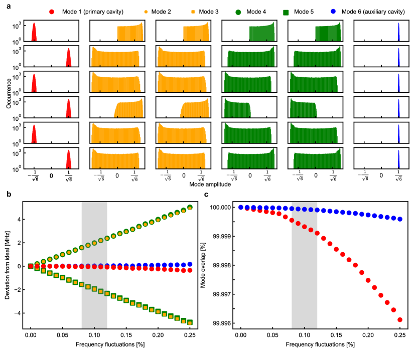
Figure S2: Statistical analysis of microwave frequency disorder. a, Eigenmode distribution for $10^{5}$ realization of Eq. (10) with frequency fluctuations sampled with a zero-mean Gaussian distribution and a variance of 0.26%. b, Average eigenfrequencies of $10^{5}$ realization of Eq. (10), where the microwave resonators frequency is randomly selected by a Gaussian distribution. It is plotted versus the Gaussian variance which represents the fabrication fluctuation. c, Average inner product (fidelity) of the mode shape of $10^{5}$ realization of Eq. (10) and the ideal case for the primary and auxiliary cavities.

We sample $10^{5}$ realization of Eq. (10) by drawing $\omega_{0}$ from a Gaussian distribution for each value of frequency disorder. The average of the microwave mode frequencies as a function of the individual resonator frequency fluctuation is shown in Fig. S2b. Small perturbations break the degeneracy of the modes, and the difference between the new eigenfrequencies increases linearly with the frequency disorder. However, the frequencies of the primary and auxiliary cavities shift 1 order of magnitude less compared with the aforementioned modes. By taking into account that the separation of modes -1 and 1 (-2 and 2) is 3 (4) MHz, from this study we can infer that the frequency fluctuations in the fabrication process are $\approx 0.1\%$. It is worth noticing that such low disorder implies a very precise control of the vacuum gap capacitors. In addition, we can use the average value of mode -1 and 1 (-2 and 2) to infer the frequency of such modes in absence of noise.

In Fig. S2c, we study the fidelity of the mode shape of the primary and auxiliary cavities compared to the ideal case, defined as $F={\left|{\left\langle{{{\psi_{{\rm{ideal}}}}}}\mathrel{\left|{\vphantom{{{\psi_{{\rm{ideal}}}}}{{\psi_{{\rm{sim}}}}}}}\right.\kern-1.2pt}{{{\psi_{{\rm{sim}}}}}}\right\rangle}\right|^{2}}$, where $\left|{{\psi_{{\rm{ideal}}}}}\right\rangle$ and $\left|{{\psi_{{\rm{sim}}}}}\right\rangle$ stand for the ideal and the simulated modeshapes, respectively. We verify that these two modes are not affected significantly by frequency fluctuation. We sample $10^{5}$ realization of Eq. (10) by drawing $\omega_{0}$ from a Gaussian distribution for each value of frequency disorder and calculate the fidelity. For fluctuation of 0.1%, we expect that such modes are $>99.9\%$ overlapping with the ideal case.

3.2 Degenerate mechanical oscillators

In section 2.4, we provided the theoretical grounds for appearance of the bright collective mode. Here, we show numerically the linewidth of the collective modes as a function of the average of cooperativities. The eigenvalues of the system and their corresponding eigenvectors can be found by diagonalizing the matrix $\bf{M}$ in Eq. (33). Similar to our device, we consider $N=6$. The simulation parameters are similar to the actual device parameters given in Tables 1 and 2. The result can be seen in Fig. S3a.

In Fig. S3a, the collective modes’ linewidths (twice of the real part of the eigenvalues of the matrix $\bf M$) are plotted versus the average of the cooperativities $\mathcal{\bar{C}}$. We see an increase in the effective linewidths only for one of the eigenmodes. The rest (5 modes) are dark, as their linewidths do not change by increasing the power. In this figure, we also plot with a dashed line 6 times of the average of the optomechanical damping rates of individual mechanics. As it is elaborated in Sec. 2.4, it can predict the behavior of the bright collective mode.

When the linewidth of the bright collective mode becomes comparable with the linewidth of the cavity, the two enter the strong coupling regime [5]. In this regime, we have hybridization between the cavity and the bright collective mode. By further increasing the power, the linewidth of the both remain constant ($\kappa/2$) and their frequencies split (Fig. S3a inset). The modeshape of the eigenmodes are found using the eigenvectors of the matrix $\bf M$ (see Sec. 6.8 for more details). The shaded region in this plot represents 90% certainty range.

3.3 Nearly-degenerate mechanical oscillators

Due to inevitable fabrication imperfections, we cannot make perfectly degenerate mechanical oscillators. In this section, we consider disorder in mechanical frequencies and linewidths, given by:

$${\Omega_{{\rm m},i}} =\Omega_{\rm m}\left({1+{\cal N}\left({{x_{i}}|\mu=0,\sigma={\sigma_{\Omega_{\rm m}}}}\right)}\right),$$ (58)

where we consider a Gaussian distribution with zero mean and $\sigma_{\Omega_{\rm m}}$ standard deviation for the frequency fluctuations. The result of simulations for two values $\sigma_{\Omega_{\rm m}}=0.001\%$ and $1\%$ can be seen in Figs. S3b and c, respectively. Considering these figures, three main regions can be defined: 1- When mechanical oscillators behave as individual mechanics, where their linewidth increase by $\Gamma_{\rm{opt},i}$ (Eq. (32)). 2- When bright collective mode appears, evidenced by linewidth increase given by $\Gamma_{\rm{opt}}=6\bar{\Gamma}_{\rm{opt,i}}$ and appearance of dark modes. 3- When strong coupling between the bright collective mode and the primary cavity occurs. This happens when linewidths of the both become equal.

The transition between regions 1 and 2 happens when the disorder between the mechanical frequencies become comparable with the optomechanical damping rates of individual mechanics. When the disorder is much larger than the optomechanical damping rates, they behave as independent mechanical oscillators. By increasing the pump power, the optomechanical damping rates increase. At a certain power, the linewidths of the mechanical oscillator become comparable to their frequency difference. This is where they interact and form the collective modes. Such condition can be written as:

$$\bar{\Gamma}_{\rm{opt,i}}=\frac{\overline{4g_{i}^{2}}}{\kappa}\simeq\frac{\bar{\Omega}_{{\rm m}}\sigma_{\Omega_{\rm m}}}{N}.$$ (59)

Considering $g_{i}=g_{0,i}\sqrt{n_{\rm p}}$, where $n_{\rm p}$ is the number of photons inside the cavity, we can write:

$$n_{\rm p}^{\rm{(1)}}\simeq\frac{\kappa\bar{\Omega}_{\rm m}}{4\overline{g_{0,i}^{2}}N}\sigma_{\Omega_{\rm m}},$$ (60)

where $n_{\rm p}^{(1)}$ stands for the required number of photons inside the cavity to observe the bright collective mode.

A transition from region 2 to region 3 occurs when the linewidth of the collective mode becomes comparable with the cavity linewidth, meaning:

$$N\bar{\Gamma}_{\rm{opt,i}}\simeq\kappa,$$ (61)

so

$$n_{\rm p}^{\rm{(2)}}\simeq\frac{\kappa^{2}}{4\overline{g_{0,i}^{2}}N},$$ (62)

where $n_{\rm p}^{(2)}$ stands for the required number of photons inside the cavity to observe strong coupling between the bright collective mode and the microwave cavity.

We aim to observe the bright collective mode before the onset of strong coupling, so it requires $n_{\rm p}^{(1)}<n_{\rm p}^{(2)}$, leading to:

$$\sigma_{\Omega_{\rm m}}<\frac{\kappa}{\bar{\Omega}_{\rm m}}.$$ (63)

This means the frequency fluctuations, $\bar{\Omega}_{\rm m}\sigma_{\Omega_{\rm m}}$, should be less than the linewidth of the cavity.

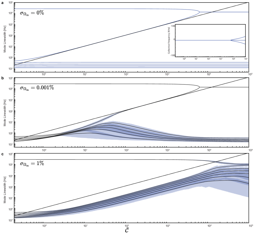
Figure S3: Effect of mechanical disorder. a-c Collective mode linewidths by finding real parts of eigenvalues of matrix $\mathbf{M}$ for mechanical disorders $\sigma_{\Omega_{\rm{m}}}=0\%,\;0.001\%\text{, and }1\%$, respectively, versus average of cooperativities. The dashed line shows 6 times of the average of optomechanical damping rates of individual oscillators. The shaded region represents 90% certainty region.

Supplementary Note 4.   Fabrication

4.1 Using DUV stepper instead of direct laser writer

In contrast to our previous works [6, 7], here we use DUV stepper (ASML PAS 5500/350C) instead of direct laser writer (Heidelberg MLA 150) for all the lithography steps. The main motivation is the better uniformity of the defined patterns as well as the higher resolution of the tool. The stepper offers better uniformity $<15$ nm ($<120$ nm for MLA), better resolution 200 nm (1 $\mu\rm{m}$ for MLA). Importantly, MLA suffers from 500 nm Field Stitching Accuracy (FSA) and 1 $\mu\rm{m}$ Blanket Stage Accuracy (BSA), which may generate some jagged boundaries when defining patterns. As we are aiming for making identical trenches (identical frequencies) for mechanical oscillators, we decide to use DUV for lithography steps. As a result, we achieve 0.1% disorder among the mechanical frequencies, an order of magnitude less than our previous work [7].

4.2 Details of the nano-fabrication process

The full fabrication process flow is reported in Fig. S4 and can be divided in four main lithography steps: patterning of the trenches, definition of bottom electrodes, planarization and vias, and finally patterning of top electrode.

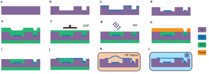
Figure S4: Main steps in the fabrication process. a, The fabrication starts with a high-resistivity silicon wafer. We then etch a trench b and deposit aluminum c. The aluminum is patterned with a wet etching process d followed by deposition of the $\rm{SiO_{2}}$ sacrificial layer. The topography is removed by chemical mechanical polishing (CMP, f). We reach to the surface of the silicon using ion beam etching g. The top and bottom layer are galvanically connected by re-flowing the resist h and etching the sacrificial layer with a 1:1 DRIE etching method i. The top aluminum electrode is deposited and then patterned with a wet etching method j. The sacrificial layer is removed using HF vapor k. At cryogenic temperatures, the top layer becomes flat l due to the tensile stress of the material.

Patterning of trenches. The fabrication starts by measuring the bow (Toho Technology FLX 2320-S) of a 4” intrinsic Silicon wafer (Topsil GlobalWafers). After logging the average bow value $<\pm 1\,\mu$m the wafer goes through standard rinse dry (SRD) with deionized (DI) water. The wafer is loaded in an automatic coater/developer (Tokyo Electron Cleantrack ACT 8) followed by a vapour deposition of HMDS and a spin-coating of 1 $\mu$m of M35G. After baking the resist at 130 degrees Celsius for 90s, the trenches and alignment markers are exposed with intensity of 21 mJ/cm² and 0 focus offset in a DUV stepper (ASML PAS 5500/350C) through a commercially produced reticle (Compugraphics). Due to the limited space on the mask, only 4 different chip layouts can be realized. The resist goes though a post exposure backing at $130^{\circ}$ C for 90 s and is automatically developed in a TMAH-based solution (JSR TMA238WA) for 60 s followed by SRD. To ensure complete removal of the resist from the exposed zones, the wafer is exposed to 200W-generated oxygen plasma (Tepla GiGAbatch) for 20 s, removing $\approx 80$ nm of resist. The exposed pattern is transferred to 350 nm trenches in the Silicon by Deep Reactive Ion Etching (Alcatel AMS 200 SE) using $\rm C_{4}F_{8}$ gas for 26 s. After such process the top layer of the resist is removed with 2 minutes of 200W-generated oxygen plasma. Any possible additional organic residue is removed by two baths of Remover 1165 at 70 degree Celsius for 5 minutes each, followed by two 5 mins dip in $100^{\circ}$ C Piranha solution, and finally rinsing in DI water. A sketch of the wafer cross section at this stage is shown in Fig. S4b.

Definition of bottom electrodes. The wafer is loaded in an electron beam evaporator (Alliance-Concept EVA 760) where 100 nm of high purity aluminum is deposited on the surface of the wafer (see Fig. S4c). After a SRD, the wafer is loaded in the automatic coater/developer where it is dehydrated in air on a hot plate at $160^{\circ}$ C and a $1\,\mu$m layer of DUV resist (M35G) is spin-coated and baked at 140 degrees Celsius for 90s. The pattern for the bottom layer is exposed in the DUV stepper with a dose of 25 mJ/cm² and 0 focus offset. After a post-exposure baking step at $140^{\circ}$ C for 90 s, it is automatically developed in a TMAH-based solution (JSR TMA238WA) for 60 s followed by SRD. To ensure complete removal of the resist from the exposed zones and to make the surface hydrophilic, the wafer is exposed to 200W-generated oxygen plasma for 20 s, removing $\approx 80$ nm of resist. The aluminum is then etched with a commercial solution of Phosphoric, Nitric, and Acetic acid (TechniEtch Al80) at $35^{\circ}$ C for 35 s, and the resist is chemically removed by dipping the wafer for 5 mins in two baths of Remover 1165 at 70 degree Celsius, followed by dipping it in DI water, and 10 s Oxygen plasma at 200 W to ensure all the resist is removed from the metal surface, as shown in Fig. S4d.

Next, we need to define the labels for each chip in the wafer. This cannot be done with DUV. Instead, we use MLA for defining the labels. The wafer is loaded in a automatic coater/developer (Süss ACS200 GEN3), vapor coated with HMDS, spin coated with $1.5\,\mu$m of positive photoresist (AZ ECI 3007), and finally soft-baked at 100 degrees Celsius for 60 s. The wafer is then mounted on the vacuum stage of a Mask-less Aligner (Heidelberg MLA 150) and chip label patterns are exposed to the resist with an intensity of 170 mJ/cm² and zero focus offset. After a post exposure backing at $110^{\circ}$ C, the resist is developed with TMAH-based solution (AZ 726 MIF) for 47 s. After an oxygen plasma step of 20 s at 200 W, the chip labels are etched into the aluminum with wet etching.

Planarization and vias. At this stage $2\,\mu$m layer of $\rm SiO_{2}$ is deposited using low thermal oxide (LTO) deposition at $425^{\circ}$ C with a mixture of silane ($\rm SiH_{4}$) and oxygen in a furnace (Centrotherm). The oxide maps the same topography seeded by the wafer, resulting in trenches on its surface; notice that a similar layer of oxide is deposited on the backside of the wafer (see Fig. S4e). In order to planarise the surface of the oxide, we use chemical mechanical polishing (CMP) for 8 mins (ALPSITEC MECAPOL E 460), with a low rate of PH-neutral slurry (ultra-sol 7A) removing $\approx 1.2\,\mu$m of the oxide as highlighted in Fig. S4f. To reach the silicon surface, we physically etch the remaining 800 nm of silicon oxide by argon ion beam etching (IBE,Veeco Nexus IBE350) for 12 minutes (see Fig. S4g). The following steps requires to galvanically connect top and bottom electrodes; after a SRD, the wafer is loaded in the DUV automatic coater. It is first coated with HMDS vapor followed by spin-coating of $1\,\mu$m layer of DUV resist (M35G) and baking at 140 degrees Celsius for 90s. The pattern for the bottom layer is exposed in the DUV stepper with a dose of 21 mJ/cm² and 0 focus offset. After a post-exposure baking step at $140^{\circ}$ C for 90 s, it is automatically developed in a TMAH-based solution (JSR TMA238WA) for 60 s followed by SRD. In order to avoid resist residues in the developed areas, the sample is exposed to oxygen plasma at 200 W for 20 s. In order to obtain a smooth surface as depicted in Fig. S4h, the resist is re-flowed for 90 s at $170^{\circ}$ C in a pre-heated oven (Heraeus T6060). We then use a 1:1 deep reactive ion etching (DRIE, SPTS APS) to transfer the pattern of the resist to the oxide (Fig. S4i). After etching, the resist is removed similar to the previous steps.

Patterning of top electrode. The sample is now loaded in the load lock chamber of an ultrahigh-vacuum electron evaporator (Plassys MEB550SL3 UHV) reaching a base pressure of $5\cdot 10^{-8}$ mTorr. At this point, a Kaufman gun is turned on for 4 mins at 400 V to Argon-mill the native oxide of the aluminum. After transferring the wafer to the deposition chamber and reaching a base vacuum of $5\cdot 10^{-9}$ Torr, 200 nm of aluminum is deposited on the surface of the wafer. The top layer is then patterned with DUV (similar to the bottom layer electrodes) and etched using the same wet etching method. After etching, the resist is removed with the standard recipe.

Dicing. The wafer is now ready for dicing. We coat 1.5 $\mu m$ resist AZ 3007 for protecting the wafer during dicing. We then dice the wafer into $5\;\rm{mm}\times 5\;\rm{mm}$ chips (Disco DAD321).

HF releasing After inspecting the samples, we remove the resist by dipping them in the wet remover followed by dipping in DI water and 2 mins of oxygen plasma. The sacrificial layer ($\rm{SiO_{2}}$) is then removed by Hydrofluoric acid (HF) vapor (SPTS uEtch), which is a dedicated tool for suspending MEMS structures.

Bonding The chips are glued to the sample holder with a butyral-phenol based glue and bonded with aluminum wires (F&S Bondtec 56i). The sample is then connected to the mixing chamber of a dilution refrigerator. Due to the tensile stress of the material at cryogenic temperatures, the top layer will be flat (Fig. S4j).

Supplementary Note 5.   Characterization

5.1 Measurement of the single photon optomechanical coupling rates ($g_{0,i}$)

To measure the single photon optomechanical coupling rates ($g_{0,i}$) of all the mechanical oscillators coupled to the primary cavity, we use a resonant weak pump on the primary cavity (Fig. S5a) to measure the upper and lower motional sidebands using a spectrum analyzer [8, 6]. The weak pump ensures that its backaction on the mechanical oscillators is negligible, i.e. $n_{{\rm{ba}},i}\equiv\frac{{4g_{0,i}^{2}}}{{\kappa\Gamma_{{\rm{m}},i}}}\frac{{(4{\kappa_{{\rm{ext}}}}/{\kappa^{2}}){P_{{\rm{MW}}}}}}{{1+{{(2\Omega_{{\rm{m}},i}/\kappa)}^{2}}}}\ll n_{{\rm{m}},i}^{{\rm{th}}}$, where $n_{{\rm ba},i}$ is the equivalent backaction noise in the unit of quanta and $P_{\rm MW}$ is the microwave input power to the device at the cavity center frequency [9].

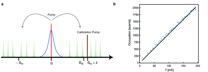
Figure S5: $g_{0}$ Measurement. a, Measurement scheme for finding $g_{0}$ of all the mechanical oscillators. b, Thermalization of the lowest frequency mechanical oscillator when we fit linearly to high temperatures $T>100$ mK.

The pump signal passes through attenuation lines in the fridge to reach the device, and then it is amplified using a HEMT at 4K stage followed by more amplifications using room temperature amplifiers (see Fig. S9 for the details of the experimental setup). The total attenuation and amplification in the measurement chain is unknown; therefore, we send an additional weak calibration pump located at the upper motional sideband, which passes through the same lines as the resonant pump. Using nominal values for the resonant/calibration pump powers at sources, $P_{\rm MW}^{\rm src}$ and $P_{\rm cal}^{\rm src}$ respectively, together with the measured calibration pump power at the spectrum analyzer and the power of the upper motional sideband of the $i$th oscillator, $P_{\rm cal}^{\rm meas}$ and $P_{{\rm SB},i}^{\rm meas}$ respectively, we can write:

$$\frac{P_{{\rm SB},i}^{\rm meas}}{P_{\rm MW}^{\rm src}}\frac{P_{\rm cal}^{\rm src}}{P_{\rm cal}^{\rm meas}}=4g_{0,i}^{2}n_{{\rm m},i}\frac{(\kappa_{\rm ext}/\kappa)^{2}}{\Omega_{{\rm m},i}^{2}+((\kappa_{\rm ext}-\kappa_{0})/2)^{2}}\frac{\omega_{\rm c}}{\omega_{\rm c}+\Omega_{{\rm m},i}}.$$ (64)

By sweeping the fridge temperature, we can approximate $n_{{\rm m},i}\simeq\frac{k_{B}T}{\hbar\Omega_{{\rm m},i}}$, where $k_{B}$ is the Boltzmann constant. At each fridge temperature, we measure the sidebands of all the mechanics. Now, with a linear fit to the power of the sideband versus temperature and using Eq. (64), we find $g_{0}$ of all the mechanical oscillators. All the values for the mechanical oscillators are given in Table 2. The thermalization of the lowest frequency mechanical oscillator is given in Fig. S5b when we fit linearly to $T>100$ mK, where the thermalization is more accurate. It is worth mentioning that the measured $g_{0}$ is less than that of a single optomechanical system by a factor of 6, as it is elaborated in Sec. 2.3.

5.2 Microwave cavity heating

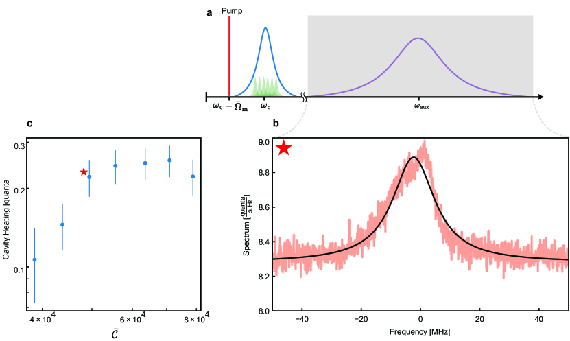
Figure S6: Cavity heating of the auxiliary cavity. a, Measurement scheme for finding cavity heating of the auxiliary cavity by pumping on the red sideband of the primary cavity. b, Detected spectrum by subtracting HEMT background and calibrating it. c, Inferred cavity heating by sweeping pump power.

By applying a strong pump on the red sideband of the primary cavity, we observe heating of the auxiliary cavity. Characterizing such heating is necessary for the sideband asymmetry experiment [6] (Sec. 6.10). To measure it, we pump on the red sideband of the primary cavity while there is no pump at the auxiliary cavity (Fig. S6a). Using a spectrum analyzer around the auxiliary cavity, we can find its spectrum $\bar{S}_{\rm c}(\omega)$ and subtract it from the HEMT background (which is found by turning off all the pumps). An example is provided in Fig. S6b. The background of the spectrum is calibrated as elaborated in Sec. 6.7. The heating of the auxiliary cavity, in the units of quanta, is then obtained [6]:

$${n_{\rm{aux}}}=\frac{{\int_{-\infty}^{+\infty}{{{\bar{S}}_{\rm{c}}}(\omega)d\omega}}}{{2\pi{\kappa_{\rm{ex}}^{\rm aux}}}},$$ (65)

where $\kappa_{\rm ex}^{\rm aux}$ is the external coupling rate of the auxiliary cavity. The result for a range of cooperativities is given in Fig. S6c.

It is worth mentioning that in the sideband asymmetry experiment Sec. 6.10, another pump is present at the auxiliary cavity, which may generate additional heating. However, we do not observe a background change around the sidebands. Hence, we used only data in Fig. S6c for analysing the data of sideband asymmetry experiment.

Supplementary Note 6.   Experimental details

6.1 Design and Simulations

The design of the microwave resonators and the feedline is carried out by simulating the electromagnetic response with a commercial method-of-moments solver (SONNET®). Setting the purely real dielectric constant to $\epsilon_{r}=11.9$ for the silicon substrate, the simulated phase of the scattering parameter $S_{11}(\omega)$ is fitted to extract the electromagnetic mode frequencies and external coupling rates (see Fig. S8). From the simulation of individual microwave resonators (as shown in Fig. S7a for the resonator closest to the feedline), we expect an average resonance frequency of $\omega_{0}^{\rm sim}/2\pi=5.45\pm 0.03$ GHz.

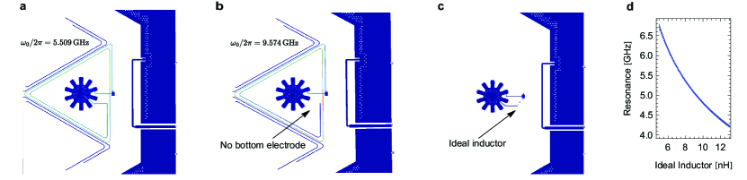
Figure S7: Simulation of the microwave response of a single resonator. a, Simulation of individual microwave resonator, where only the close sections of the inductors are left, giving a resonance frequency close to $\omega_{0}^{\rm sim}/2\pi=5.5$ GHz. b, In order to estimate the stray capacitance, the same simulation is repeated after removing the bottom electrode, yielding a larger resonance frequency around $\omega_{0,{\rm nodrum}}^{\rm sim}/2\pi=9.6$ GHz. c The estimation of the drum capacitor is performed by simulating the resonance frequency as a function of the inductance of an ideal inductor. The results are reported in d.

To extract the value of stray capacitance we take the ratio between the resonator with and without bottom electrode (as shown in Fig. S7b):

$$\left(\frac{\omega_{0}^{\rm sim}}{\omega_{0,\rm nodrum}^{\rm sim}}\right)^{2}=\frac{C_{\rm s}}{C_{\rm d}+C_{\rm s}}\approx 0.32,$$ (66)

so 68% of the total capacitance is localized between the top drum and bottom electrode. In addition, by simulating the resonance frequency of an ideal inductor shunted by a vacuum gap capacitor, we can determine the value of both stray capacitance $C_{\rm s}=37.3$ fF and vacuum gap capacitance $C_{\rm d}=75.2$ fF (see Fig. S7c and d).

We also simulate the full system to ensure the equal distribution of the symmetric and anti-symmetric modes. The phase of the reflection coefficient is reported in Fig. S8a.

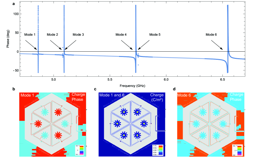
Figure S8: Microwave simulation of the full circuit. a, Simulated phase of the $S_{11}$ reflection coefficient as a function of driving frequency to the microwave feedline. The arrows highlight the frequencies of each modes. b-d, Choosing the driving frequency of modes 1 or 6, the simulation shows the preserved symmetry in charge distribution and its phase.

The reflection remarkably shows 6 individual modes. The splitting of the modes 2 and 3 (4 and 5), that would be degenerate in the ideal case, is 40 MHz, which is one order of magnitude larger than the experimentally measured one. We attribute this deviation to discretization error while meshing the metallic layout, where $2\times 2\,\mu\rm m^{2}$ elements are used. Despite this large numerical errors, we qualitatively asses the mode shape of the primary and auxiliary cavities, by plotting the charge phase in Figs. S8b and d respectively. Finally, the charge distribution, that represents the microwave occupation of each individual resonators, is reported in Fig. S8c and it identical for both modes.

6.2 Experimental setup

The schematic of the full setup, room temperature (RT) and cryogenic, is illustrated in Fig. S9.

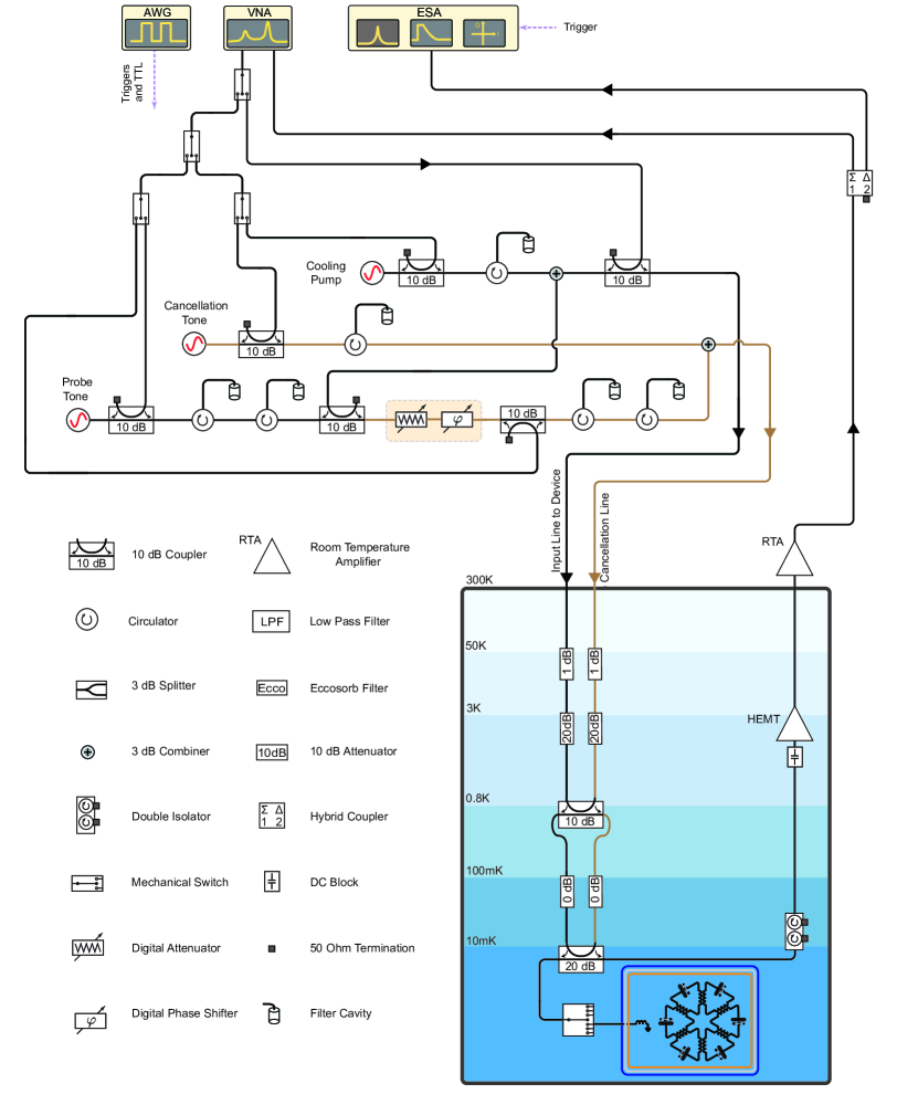
Figure S9: Complete cryogenic and room temperature setup. Black lines are the main signal path to the device and brown lines are the tone cancellation lines. Solid-state switches are not shown in this schematic.

For OMIT and ground state cooling experiment, we use a VNA (Rohde & Schwartz, ZNB 20) together with a strong pump (Cooling Pump on the figure, Rohde & Schwartz, SMA100B), which is red-detuned from the primary cavity. The pump is routed to the device through an attenuated line in the fridge and a cryo-switch (Radiall, R583-423-141) in the mixing chamber. The reflected signal (together with the sidebands) passes through a dual-junction isolator (Low Noise Factory, LNF-ISISC4 8A) and is amplified at 3K stage of the fridge using a high-electron-mobility transistor (HEMT: Low Noise Factory, LNF-LNC4-8C). Finally, it is amplified at RT (Low Noise Factory, LNF-LNR1-15A-SV) and goes to a VNA and an electrical spectrum analyzer (ESA: Rohde & Schwartz, FSW) for detection. Frequency-tunable motorized filter cavities [10] are used to remove phase noise of the source at anti-Stokes sideband, as it may increase the mechanical occupation [11]. The power of the cooling pump can reach very high values, $\approx 27$ dBm at RT, which may saturate the HEMT. To avoid it, the cooling pump signal needs to be canceled before the HEMT. In our experiment, we use another source, (Cancellation Tone on the figure, Rohde & Schwartz, SMA100B), which interferes destructively with the cooling pump signal after the device. The frequency of this source is similar to the cooling pump, and its phase and power are swept to maximize the cancellation. We do not use a digital phase shifter and an attenuater [6], as these devices have $\approx 13$ dB loss, preventing us from reaching high cooperativities necessary for this experiment.

For performing the sideband asymmetry experiment, we use another probe tuned on the auxiliary cavity center frequency (Probe Tone on the figure, Rohde & Schwartz, SMF100A). The power of this tone is moderate, hence we use a digital phase shifter and attenuater to cancel it after the device. Because we measure both the Stokes and anti-Stokes sidebands, we use two filter cavities tuned on the upper and lower motional sidebands. We use another pair of filter cavities after the tone cancellation branch to remove any added noise due to this branch. To monitor the filter cavities and the device, we rout the VNA signal through all the lines using mechanical switches (Mini-Circuits, MSP2T-18XL+).

For the modeshape measurement experiment, we change the experimental setup by removing digital attenuators/phase shifters and using the probe tone as the excitation signal (see Fig. 3 of the main text). For making pulses, we use solid-state switches (Mini-Circuits, ZFSWA2R-63DR+) after the cooling pump, cancellation tone, and probe tone which have $\approx 35$ ns rising/falling time and can be controlled with TTL generated by an arbitrary wave generator (AWG: Tektronix, AFG3252C). Considering the switching time of these switches, the uncertainties of the modeshape phase is $\Delta\varphi\simeq 2\pi\times 5\;\rm{kHz}\times 35\;{\rm ns}=2\;\rm{mRad}$, which is acceptable in our experiment.

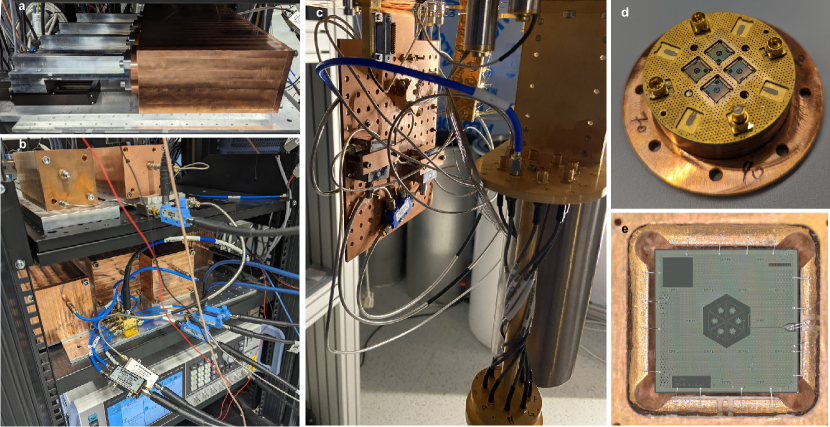
Figure S10: Details of the experimental setup. a and b, filter cavities for removing the phase noise of the sources. c, cold fingers for connecting the sample to the mixing chamber. d, sample holder with four bounded chips. e, bounded chip to the sample holder.

As shown in Fig. S9 the experiments require careful phase noise cancellation that is achieved by employing 6 filter cavities whose frequencies can be tuned remotely using stepper motors (see Fig. S10a). A photograph of their inclusion in the experimental setup is shown in Fig. S10b.

The sample is thermally and mechanically anchored at the mixing chamber stage of a dilution fridge (BLUEFORS, LD250) with an average base temperature of 10 mK. The cold fingers which connect the device to the mixing chamber (see Fig. S10c) are enclosed on a triple layer shield of $\mu-$metal, eccosorb, and copper, which protect the sample microwave environment [12]. The cryogenic microwave components are placed on a copper plate. The sample is bonded to a trilayer goldplated PCB, which is mounted on a copper plate that hosts four chips as shown in Fig. S10d. We keep the number of bonds per side to four to minimize the possible effect of the ultrasonic vibration of bonding on the metallic drums (Fig. S10e).

6.3 Attenuation scheme and photon occupation

Two attenuated lines are used to rout a driving tone to the device and to destructively interfere this tone to prevent the HEMT amplifier saturation. Importantly, attenuations in the last three stages (still, cold plate, and mixing chamber plate) have been removed to avoid their thermal overload when a strong pump is sent. However, the photonic bath of such lines is kept cold by adding directional couplers instead of attenuators. While a more optimized case would dump the excess driving power in a third line towards higher stages, the limited lines available in our dilution refrigerator constrained our experiment to use only these two.

In the presented scheme, the estimation of the total attenuation as well as the photon bath occupation slightly deviates from the simple case of attenuators, because the signal in a single branch travels back and forth between the stages. For example, considering the ideal case of two couplers in series with coupling $A_{1}$ and $A_{2}$, respectively, without accounting for line intrinsic attenuation or connector loss, or the length of the connections, in the steady state, the transmittance $S_{21}=V_{\rm out}/V_{\rm in}$ can be calculated as

$$S_{21}=A_{1}A_{2}\sum_{n=0}^{\infty}\left[(1-A_{1})(1-A_{2})\right]^{n}\approx\frac{A_{1}A_{2}}{A_{1}+A_{2}}.$$ (67)

This attenuation maximizes to $A/2$ when $A_{1}=A_{2}=A$. The total nominal attenuation in our setup is 42dB, while taking into account 1dB connection loss for all components, we have a total attenuation of approximate 50dB, resulting in the total photon number of 0.09 and 0.07 at 4.8 GHz and 6.2 GHz, respectively.

Finally, it is worth mentioning that the consecutive couplers give rise to a Fabri-Perot resonant condition, as in fact measured experimentally (see Sec. 6.4 for mode details).

6.4 Microwave modes characterization

The values reported in Sec. 1 are obtained by fitting the microwave reflection $S_{11}(\omega)$ for all the microwave modes. In particular, we remove the microwave background due to imperfection in our experimental setup (see Sec. 6.2 for more details).

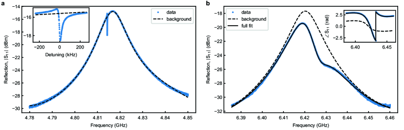
Figure S11: Characterization of the microwave modes. a, Amplitude of the reflection coefficient for the primary cavity. The fit to the background (dashed line) clearly capture the behaviour of the main feature of the signal. In the inset, we show the comparison between the estimated background near the mode resonance. b, Amplitude of the reflection coefficient for the auxiliary cavity; due to a linewidth comparable to the background feature, the background (dashed line) and the microwave mode are simultaneously fitted (solid line). In the inset we show the phase of $S_{11}$ and the fits.

In Fig. S11, we report the raw reflection data from a VNA, specifically for the primary cavity in a and the auxiliary cavity in b. For the primary cavity (and for all other modes except the auxiliary cavity), the linewidth is much narrower than the background fluctuation, so the background can be removed by fitting only the amplitude part to

$$|S_{11}^{\rm bg}|=\frac{A_{\rm bg}}{\pi\gamma_{\rm bg}(1+(\omega-\omega_{\rm bg})/\gamma_{\rm bg})^{2}}+B_{\rm bg}\cos(C_{\rm bg}\omega+\phi_{0})+D_{\rm bg}$$ (68)

which takes into account the Lorentzian-like resonance due to the reflection from two cascaded couplers as well as possible impedance mismatch. The result of the fits (dashed line) well reproduces the background that is removed to obtain each microwave mode reflection data (see inset in Fig. S11a). Such procedure is repeated for all the microwave modes except for the auxiliary cavity that requires a different fitting scheme. After subtracting the background and applying a normalization, the reflection $S_{11}(\omega)$ is fitted to

$$S_{11}=\exp{\left(i\omega\tau-i\alpha_{i}\right)}\left(1-\frac{2\kappa_{\rm ex}^{i}e^{i\phi}}{\kappa_{\rm ex}^{i}+\kappa_{0}^{i}+2i(\omega-\omega_{i})}\right)$$ (69)

and the results are reported in Figure 1 in the main text.

For the auxiliary cavity, due to its large linewidth, it is not possible to fit independently the background. In order to extract this mode parameters, we fit the complex reflection coefficient:

$$S_{11}^{\rm combined}=\left(\frac{A_{\rm bg}\exp{\left(i\omega\tau-i\alpha_{\rm bg}\right)}\sqrt{\kappa_{\rm i,bg}\kappa_{\rm ext,bg}}}{\kappa_{\rm tot,bg}+2i(\omega-\omega_{\rm bg})}+B_{\rm bg}\cos(C_{\rm bg}\omega+\phi_{0})+D_{\rm bg}\right)S_{11},$$ (70)

where the background in this case is modeled as a resonator in trasmission cofiguaration, hence the three coupling terms $\kappa_{\rm i,bg}$, $\kappa_{\rm ext,bg}$ and $\kappa_{\rm tot,bg}$ . Figure S11b display the magnitude and the phase (inset) as well as the fit (in solid line). Using the fitted values, the reconstructed background is shown in the dashed line.

6.5 Microwave nonlinearities

In our optomechanical model, we assume that fourth order Kerr nonlinearity, $K$, in the microwave modes has negligible effect in the photon number regime produced by the pumping powers used in all experiment. To confirm this assumption, here we characterize the Kerr effect as a function of intra-cavity photon number for the primary cavity mode. We use a VNA and measure the amplitude and phase of the reflection coefficient $S_{11}(\omega)$ reported in Figs. S12a and b, respectively.

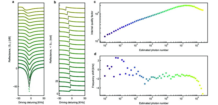
Figure S12: Microwave response of the primary cavity as a function of driving power. a, Magnitude and b phase of the reflection coefficient $S_{11}$ of the primary cavity mode as a function of power drive (each trace is shifted by 9 dB and 9 rad to make them visible). c, Internal quality factor and d resonance frequency extracted by fitting the complex $S_{11}$ to the model in (71) as a function of the inferred intra-cavity photon number. The color code shows the intra-cavity photon number.

Following the treatment in [13] and assuming a total cryogenic attenuation of 50 dB, we fit all traces with a modified expression for the reflection coefficient,

$$S_{11}=\exp{\left(i\omega\tau-i\alpha_{i}\right)}\left(1-\frac{2\kappa_{\rm ex}e^{i\phi}}{\kappa_{\rm ex}+\kappa_{\rm 0}+2i(\omega-\omega_{\rm c})+i\frac{|\alpha_{\rm in}|^{2}K}{\kappa_{0}+\kappa_{\rm ex}}n}\right),$$ (71)

that takes into account the nonlinear relation between the driving power $P_{\rm in}$ and the intra-cavity photon number due to the Kerr term. Here, by using the driving field $\alpha_{\rm in}=P_{\rm in}/\hbar\omega$ and the intra-cavity coherent field $\alpha$, the parameter $n=|\alpha|^{2}/|\alpha_{\rm in}|^{2}$ is obtained by solving the third order algebraic equation for each driving power

$$\left[\left(\frac{\omega_{\rm c}-\omega}{\kappa_{0}+\kappa_{\rm ex}}\right)^{2}+\frac{1}{4}\right]n-2\frac{\omega_{\rm c}-\omega}{(\kappa_{0}+\kappa_{\rm ex})^{2}}Kn^{2}+\left(\frac{K}{\kappa_{0}+\kappa_{\rm ex}}\right)^{2}n^{3}=\frac{\kappa_{0}}{\kappa_{0}+\kappa_{\rm ex}}.$$ (72)

The model well reproduces the experimental data. The internal quality factors and the resonance frequencies extracted from the fit are reported in Figs. S12c and d, respectively. The strong power dependence of the quality factor suggests that at low intra-cavity photon numbers, the primary cavity mainly dissipates via the two-level systems bath located between the capacitor electrodes; such behavior has been already observed in the literature for vacuum gap capacitors [14, 15]. At intermediate powers, the resonance frequency is constant within the experimental errors, while the Lorentzian dip shifts (compare Fig. S12b and d). This is due to the presence of small Kerr nonlinearity ($K/2\pi<1\;{\rm Hz}$) whose effect appears for large photon numbers. Finally above $10^{8}$ photons, the resonance frequency shifts and the quality factor slightly degrades. We attribute such behavior to quasi-particles generation in the inductors that results in a lossy resonator.

6.6 Microwave thermal response

In this section, we study the single microwave tone response of the primary cavity as a function of the mixing chamber temperature, to which the sample is thermally anchored. We drive the cavity by a single coherent tone generated by a VNA and measure the amplitude and phase of reflection coefficient $S_{11}$ reported in Figs. S13a and b, respectively.

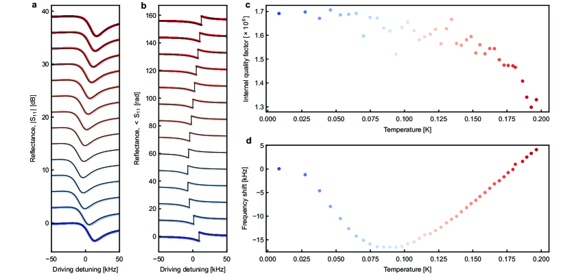
Figure S13: Microwave response of the primary cavity as a function of temperature. a, Magnitude and b phase of the reflection coefficient $S_{11}$ of the primary cavity mode as a function of mixing chamber temperature (each trace is shifted by 9 dB and 9 rad to make them visible). c, Internal quality factor and d resonance frequency extracted by fitting the complex $S_{11}$ to the linear model as a function of the temperature. The color code shows the mixing chamber temperature.

As expected [16], the quality factor of aluminum resonators degrades due to quasi-particle poisoning when the temperature becomes a considerable fraction of the superconducting critical temperature, see Fig. S13c. In addition, for temperatures below 100 mK, the frequency of the primary cavity decreases due to an increase in broken cooper pairs, which increases the superconducting films kinetic inductance (see Fig. S13d). However, for higher temperatures, the frequency shift changes sign and increases with temperature. We attribute this effect to the relaxation of the strain in the film, resulting in the increase of the gap size, and consequently reducing the capacitance.

6.7 Noise floor calibration

To extract the occupation of the bright collective mode, we need to calibrate the noise floor of the output spectrum. We model the experimental setup after the device as given in Fig. S14a. In this model, $\eta$ is the loss between the device under test (DUT) and HEMT, $n_{\rm{add}}^{\rm{H}}$ is the added noise of HEMT, and $G_{\rm{H}}$ is the gain of HEMT. The added noise of the measurement chain after HEMT can be neglected due to its high gain. The detected signal at room temperature is then given by:

$${G_{\rm{H}}}\left({\eta s+\frac{1}{2}+n_{{\rm{add}}}^{\rm{H}}+\frac{1}{2}}\right)={G_{\rm{H}}}\eta\left({s+\frac{{1+n_{{\rm{add}}}^{\rm{H}}}}{\eta}}\right).$$ (73)

Here, $s$ is the signal leaving the device, the first $1/2$ is the vacuum noise, $n_{\rm add}^{\rm H}$ is the added noise of HEMT, and the second $1/2$ is the added noise due to phase-insensitive amplification. The background of the signal referred to the device is $1+n_{\rm add}=\frac{1+n_{{\rm{add}}}^{\rm{H}}}{\eta}$. Note that in an ideal phase-insensitive measurement $n_{\rm add}=0$.

We need then to reliably find the added noise of HEMT. To this end, we sweep the temperature of mixing chamber and wait until all the lines and devices connected to it thermalize to this temperature. In this case, the thermal input signal to HEMT is given by:

$$s_{\rm{th}}=\frac{1}{1-\exp(-\hbar\omega/k_{\rm{B}}T)},$$ (74)

where $k_{\rm{B}}$ is the Boltzmann constant and $T$ is temperature of the mixing chamber. The detected signal is given by:

$${G_{\rm{H}}}\left(s_{\rm{th}}+n_{\rm{add}}^{\rm{H}}+1\right).$$ (75)

The signal in a wide span is detected using a spectrum analyzer. We then divide the entire frequency span into sections, calculate the average noise power for each section, and plot these average values versus temperature. By fitting this curve to (75) with $n_{\rm{add}}^{\rm{H}}$ and $G$ as free parameters, we can extract $n_{\rm{add}}^{\rm{H}}$ at each frequency section. Calibration data around the primary and auxiliary cavity center frequencies are given in Figs. S14b and c, respectively. Between DUT and HEMT we have a cryo switch, which has 0.2 dB attenuation, a dual-junction isolator with 0.2 dB attenuation, and some cables with 0.8 dB attenuation. The numbers are considered from datasheet. We consider 0.5 dB systematic error for the estimated loss. The extracted added noised (referred to DUT) are then $1+n_{\rm add}=9.0\pm 1.0$ quanta and $8.3\pm 1.0$ quanta around primary and auxiliary cavity frequencies, respectively.

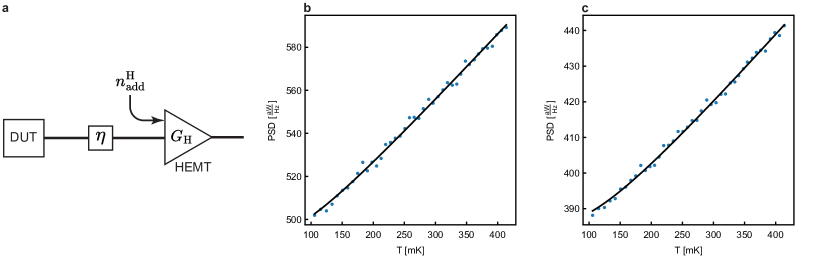
Figure S14: Noise floor calibration. a, Simplified measurement setup after the device. b and c, Calibration data for HEMT around the primary and auxiliary cavity frequencies, respectively.

6.8 Modeshape of collective modes

In order to measure the modeshapes of the collective modes, we leverage the slight non-degeneracy of the mechanical oscillator frequencies. For each pump power, we first take a VNA trace around the cavity frequency, which provides us with the multi-mode OMIT response (Sec. 2.5). We then fit Eq. (38) to data with $g_{i}$s, $\kappa$, and $\omega_{\rm{c}}$ as free parameters. Using these parameters, we constitute the matrix $\bf M$ in Eq. (33). Then, we find eigenvalues of this matrix, which are complex valued parameters. The real parts are half of the mode linewidths and the imaginary parts are the mode frequencies. Afterwards, for each pump power, we send an excitation signal that is blue detuned from the pump by each mode frequency. The beating of these two tones will excite selectively the target mode. In the basis of the individual mechanical oscillators, each oscillator will be excited based on its participation ratio in the excited collective mode. To measure these amplitudes, we turn off both the pump and the excitation signal and send a weak pump which is red detuned from the cavity by the average of the bare mechanical frequencies. The power of the pump is weak enough to ensure that $\left|{{\Omega_{{\rm{m}},i}}-{\Omega_{{\rm{m}},j}}}\right|\gg{\Gamma_{{\rm{opt,}}i}},{\Gamma_{{\rm{opt,}}j}}$ and high enough to ${\Gamma_{{\rm{opt,}}i}}\gg{\Gamma_{{\rm{m,}}i}}$. This is to assure that the oscillator sidebands do not interfere, but at the same time, the rates are more than the bare damping rates. We then record both the in-phase ($I$) and out-of-phase ($Q$) quadratures of the emitted signal around the cavity frequency with sampling rate 50 kHz using the I-Q mode of a spectrum analyzer. The sampling rate is chosen so that all the ringdowns of the mechanical oscillators can be recorded (they all fall in a span as low as 10 kHz). Having both $I$ and $Q$ of the signal enable us to extract the phase of the collective mode. Now, to find the participation ratio of each mechanical oscillator in the excited mode, we take a Fourier transform of the recorded signal $z(t)=I(t)+iQ(t)$. As we can see from Fig. 3 of the main text, this contains 6 peaks related to the bare mechanical oscillator frequencies. Next, we fit the following complex Lorentzian function to each of these peaks,

$$f(\omega)=\frac{A_{j}^{k}e^{i\varphi_{j}}(\Gamma_{{\rm{m}},j}/2-j(\omega-\Omega_{{\rm{m}},j}))}{\Gamma_{{\rm{m}},j}^{2}/4+(\omega-\Omega_{{\rm{m}},j})^{2}}+{\rm BG}_{j}$$ (76)

which is Fourier transform of $A_{j}^{k}e^{i\varphi_{j}}e^{(-i(\omega-\Omega_{{\rm{m}},j})-\Gamma_{{\rm{m}},j}/2)t}\theta(t)$, where $A_{j}^{k}$ is ringdown amplitude of the $j$th mechanical oscillator of the $k$th excited collective mode, $\varphi_{j}^{k}$ is its phase, ${\rm BG}_{j}$ is the fitting background, and $\theta(t)$ is the Heaviside function. For each pump power, we have $N+1$ eigenmodes, for each of which we follow the aforementioned procedure. The normalized amplitude can be found as:

$$\eta_{i}^{k}=\frac{{{A_{i}^{k}}}}{\sqrt{\sum\limits_{j=1}^{N}{{{\left|{{A_{j}^{k}}}\right|}^{2}}}}}.$$ (77)

Theoretical values for eigenvectors are determined by diagonalizing the matrix $\bf{M}$ in Eq. (33), utilizing the fitting parameters to the multi-mode OMIT response Eq. (38). The reconstructed modeshapes and the theoretical ones for pump cooperativities $\mathcal{\bar{C}}=328$, 2056, 13301, and 67182 are given in Figs. S15a-d, respectively, where a great overlap is observed, both in phases and amplitudes. It is worth mentioning that in the reported modeshapes, we have ignored the mode with the largest linewidth, as the microwave cavity has the maximum participation ratio in it.

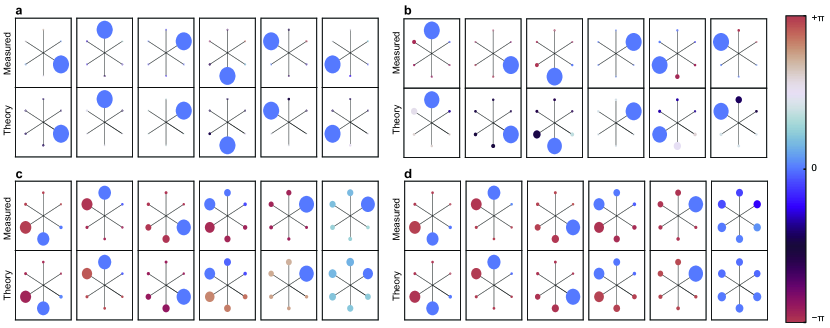
Figure S15: Collective modeshapes. a-d, Collective modeshape reconstruction for pump cooperativities $\mathcal{\bar{C}}=328,2056,13301,\;{\rm and}\;67182$, respectively. Normalized amplitudes are given by the circle radius and the phase is given by the color.

6.9 Occupation of collective and dark modes

To find the occupation of the dark and bright collective modes in the presence of a pump red-detuned from the primary cavity by $\bar{\Omega}_{\rm m}$, we need to first detect the power spectral density (Eq. (45)). Considering gain, loss, and added noise of the measurement chain 6.7, the detected spectrum is given by:

$$\bar{S}^{\prime}(\omega)=G\left({\bar{S}(\omega)+\frac{1}{2}+{n_{{\rm{add}}}}}\right).$$ (78)

Here, $G$ is the scaling factor induced by all the gain and loss of the measurement chain and $n_{\rm add}$ is the equivalent added noise of the chain referred to the device. For an ideal measurement chain (zero loss and ideal phase-insensitive measurement), $n_{\rm add}$ is zero. In our experiment, it is measured in Sec. 6.7. By knowing the background of the detected spectrum, we can find the scaling factor $G$.

We then fit Eq. (45) to the calibrated spectrum considering decoherence rates ($\Gamma_{{\rm th},i}=\Gamma_{{\rm m},i}n_{{\rm m},i}^{\rm th}$), microwave cavity frequency and linewidth, as well as coupling rates as free parameters. After finding these parameters, we plug them into Eq. (46) to find correlations among different mechanical oscillators. Having all these correlations, we can constitute the covariance matrix Eq. (52). Diagonalizing this matrix provides us with the occupations of the modes. Importantly, the Hermiticity of this matrix ensures that all the eigenvalues are real. The minimum eigenvalue corresponds to the occupation of the bright collective mode, as it has the maximum coupling to the cavity. The other eigenvalues, however, correspond to the occupation of the dark collective modes. The occupation of dark and bright collective modes together with the cavity heating versus cooperativity is plotted in Fig. S16b.

The eigenvector corresponding to each eigenvalue provides us with the mechanical modeshape of that mode. In Fig. S16b, we plot the fidelity, defined as $F(\psi_{i},\psi_{i}^{\prime})={\left|{\left\langle{{{\psi_{i}}}}\mathrel{\left|{\vphantom{{{\psi_{i}}}{{\psi_{i}^{\prime}}}}}\right.\kern-1.2pt}{{{\psi_{i}^{\prime}}}}\right\rangle}\right|^{2}}$ for two vectors $\left|{{\psi_{i}}}\right\rangle$ and $\left|{{\psi_{i}^{\prime}}}\right\rangle$, between the ideal bright collective mode (31) and the mechanical modeshapes found using eigenvectors of the covariance matrix. As it can be seen from this figure, all the fidelities start from $1/6$, meaning that they are localized in one of the mechanical oscillators. This can be also seen in Fig. S15 at low cooperativities. By increasing the pump power, the fidelity of the bright collective mode (blue circle) increases, and finally it reaches to one. The fidelity of dark collective modes, however, go to zero by increasing the pump power, meaning that they become orthogonal to the collective mode.

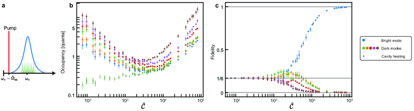
Figure S16: Occupancy of collective modes. a, Measurement scheme for finding the occupation of dark and bright collective modes. b, Occupation of dark and bright collective modes using the eigenvalues of the covariance matrix. Cavity heating is shown with small green circles. c, Fidelities between bright/dark collective modes and the ideal collective mode (31).

6.10 Sideband asymmetry

To cross verify the occupation measured using the method mentioned in Sec. 6.9, we use sideband asymmetry experiment, which is an out-of-loop measurement technique [17, 18, 6]. The extracted occupation in Sec. 6.9 depends on the noise floor calibration, which is found using fridge base temperature sweep (Sec. 6.7). The sideband asymmetry experiment, on the other hand, is independent of the noise floor and only depends on the difference between the Stokes and anti-Stokes motional sidebands. In this experiment, we use the auxiliary cavity which has a broad linewidth ($\kappa_{\rm aux}\simeq 15\;\rm{MHz}>\bar{\Omega}_{\rm m}\simeq 2\;\rm{MHz}$). By pumping on-resonant (slightly red-detuned with detuning $\Delta<0$) on this cavity, we can generate two upper (anti-Stokes) and lower (Stokes) motional sidebands whose areas are proportional to the mechanical occupations. For cooling, we use a pump on the red sideband of the primary cavity (see Fig. 4e of the main text).

Here, we perform sideband asymmetry experiment in two different regimes: 1- When the power of the cooling pump is low enough that the mechanical sidebands of individual mechanical oscillators do not interfere ($\Gamma_{{\rm{opt}},i},\Gamma_{{\rm{opt}},j}\ll\left|{{\Omega_{{\rm{m}},i}}-{\Omega_{{\rm{m}},j}}}\right|\ll\kappa$). In this case, we can consider the system as $N$ single optomechanical systems. 2- When power of the cooling pump is sufficiently high to induce the emergence of the bright collective mode and its strong coupling with the primary cavity. In this case, as we are only interested in the occupation of the bright collective mode, we can approximate the sidebands with the spectrum of a single optomechanical system in the strong coupling regime, where the mechanical oscillator is the bright collective mode. In both regimes, the cavity heating of the auxiliary cavity should be considered, as it introduces a fake asymmetry [6].

6.10.1 Sideband asymmetry of individual mechanical oscillators (low power)

In this regime, we perform the sideband asymmetry experiment on the mechanical oscillator that is furthest from the others, $\Omega_{\rm{m},1}-\bar{\Omega}_{\rm{m}}=-2\pi\times 5.19$ kHz. By using this mechanical oscillator, we can use a wider range of powers before it interferes with the other ones. By pumping on the auxiliary cavity slightly red-detuned $\Delta<0$, we generate two upper and lower motional sidebands whose areas are proportional to $\Gamma_{+}(n_{{\rm{m}},1}-2n_{{\rm aux}})$ and $\Gamma_{-}(n_{{\rm{m}},1}+1+2n_{{\rm aux}})$, respectively. Here, $n_{{\rm{m}},1}$ is the occupation of the first mechanical oscillator and

$$\Gamma_{\pm}=\frac{4g_{1,{\rm aux}}^{2}\kappa_{\rm aux}}{\kappa_{\rm aux}^{2}+4(\Omega_{{\rm m},1}\pm\Delta)^{2}},$$ (79)

where $g_{1,{\rm aux}}$ is the optomechanical coupling rate of the first mechanical oscillator to the auxiliary cavity. In the case of resonant pumping, $\Gamma_{-}=\Gamma_{+}$. We always pump slightly red-detuned ($\approx 100$ kHz) to avoid entering parametric instability regime [3]. In this case, to take into account the slight difference between $\Gamma_{+}$ and $\Gamma_{-}$, we turn off the cooling pump (red-detuned from the primary cavity by $\Omega_{{\rm m},1}$) and measure the upper and lower motional sidebands (with this, $n_{\rm{m}}\simeq n_{m}+1\gg 1$). The ratio of the areas then provides us with $\Gamma_{+}/\Gamma_{-}$. It should be noted that using a resonant pump on the auxiliary cavity will introduce backaction on the mechanical oscillator, and its effective occupation will increase given by [6]: $\frac{{{\Gamma_{-}}({n_{{\rm{aux}}}}+1)+{\Gamma_{+}}{n_{{\rm{aux}}}}}}{{{\Gamma_{{\rm{m}},1}}+{\Gamma_{{\rm{opt}},1}}+{\Gamma_{\rm{+}}}-{\Gamma_{-}}}}$. We confirm that in this regime of cooling powers, we did not observe heating of the auxiliary cavity. In addition, the mechanical sideband is fitted using a Voigt function. By finding the mechanical occupation using the calibrated background and comparing it with the sideband asymmetry experiment, we find an excellent overlap, confirming the quantum efficiency extracted in Sec. 6.7.

6.10.2 Sideband asymmetry of the bright collective mode (high power)

In this regime, the linewidth of the bright collective mode becomes comparable with the linewidth of the primary cavity, so they enter the strong coupling regime [5]. It should be noted that the linewidth of the auxiliary cavity ($\simeq 15$ MHz) is much larger than that of the bright collective mode ($\simeq 30$ kHz). We again pump the auxiliary cavity slightly red-detuned ($\Delta<0$) and pump on the red-sideband of the primary cavity (with detuning $\bar{\Omega}_{\rm m}$). Here, due to the hybridization, the upper and lower motional sidebands are given by (ignoring the narrow peaks of dark modes) [19]:

$$S(\delta)={\rm{BG}}+\frac{{A{\delta^{2}}}}{{|4{g^{2}}-4\delta(\delta+\tilde{\Delta})+2i\delta\kappa{|^{2}}}}+\frac{B}{{|4{g^{2}}-4\delta(\delta+\tilde{\Delta})+2i\delta\kappa{|^{2}}}},$$ (80)

where $\delta=\omega+\omega_{\rm aux}\pm\bar{\Omega}_{\rm m}$, $\tilde{\Delta}=\omega_{\rm p}-\omega_{\rm c}+\bar{\Omega}_{\rm m}$, $\omega_{\rm p}$ is the frequency of the pump (red-detuned from the primary cavity), and BG is the background. The $\pm$ in $\delta$ refers to the anti-Stokes and Stokes sidebands, respectively. After fitting Eq. (80) to the sidebands (as depicted in Fig. 4 of the main), we find area under each of them. Together with the cavity heating already found in Sec. 5.2, we can find the occupation of the bright collective mode, which are plotted in Fig. 4 of the main text.

The sidebands in this regime have very low signal-to-noise ratio; therefore, given that we do not have a JTWPA in our measurement chain, we averaged for 90000 times with spectrum analyze resolution bandwidth RBW = 100 Hz per sideband.

Supplementary References

References

- Anderson [1972] P. W. Anderson, More is different, Science 177, 393 (1972).
- Strogatz [2004] S. Strogatz, Sync: The emerging science of spontaneous order (Penguin UK, 2004).
- Bardeen et al. [1957] J. Bardeen, L. N. Cooper, and J. R. Schrieffer, Theory of superconductivity, Physical review 108, 1175 (1957).
- Anderson et al. [1995] M. H. Anderson, J. R. Ensher, M. R. Matthews, C. E. Wieman, and E. A. Cornell, Observation of bose-einstein condensation in a dilute atomic vapor, science 269, 198 (1995).
- Dicke [1954] R. H. Dicke, Coherence in spontaneous radiation processes, Physical review 93, 99 (1954).
- Tavis and Cummings [1968] M. Tavis and F. W. Cummings, Exact solution for an n-molecule—radiation-field hamiltonian, Physical Review 170, 379 (1968).
- Aspelmeyer et al. [2014] M. Aspelmeyer, T. J. Kippenberg, and F. Marquardt, Cavity optomechanics, Reviews of Modern Physics 86, 1391 (2014).
- Xuereb et al. [2012] A. Xuereb, C. Genes, and A. Dantan, Strong coupling and long-range collective interactions in optomechanical arrays, Physical review letters 109, 223601 (2012).
- Xuereb et al. [2013] A. Xuereb, C. Genes, and A. Dantan, Collectively enhanced optomechanical coupling in periodic arrays of scatterers, Physical Review A 88, 053803 (2013).
- Heinrich et al. [2011] G. Heinrich, M. Ludwig, J. Qian, B. Kubala, and F. Marquardt, Collective dynamics in optomechanical arrays, Physical Review Letters 107, 043603 (2011).
- Peano et al. [2015] V. Peano, C. Brendel, M. Schmidt, and F. Marquardt, Topological phases of sound and light, Physical Review X 5, 031011 (2015).
- Massel et al. [2012] F. Massel, S. U. Cho, J.-M. Pirkkalainen, P. J. Hakonen, T. T. Heikkilä, and M. A. Sillanpää, Multimode circuit optomechanics near the quantum limit, Nature communications 3, 987 (2012).
- Ockeloen-Korppi et al. [2019] C. Ockeloen-Korppi, M. Gely, E. Damskägg, M. Jenkins, G. Steele, and M. Sillanpää, Sideband cooling of nearly degenerate micromechanical oscillators in a multimode optomechanical system, Physical Review A 99, 023826 (2019).
- Teufel et al. [2011a] J. D. Teufel, T. Donner, D. Li, J. W. Harlow, M. Allman, K. Cicak, A. J. Sirois, J. D. Whittaker, K. W. Lehnert, and R. W. Simmonds, Sideband cooling of micromechanical motion to the quantum ground state, Nature 475, 359 (2011a).
- Weinstein et al. [2014] A. Weinstein, C. Lei, E. Wollman, J. Suh, A. Metelmann, A. Clerk, and K. Schwab, Observation and interpretation of motional sideband asymmetry in a quantum electromechanical device, Physical Review X 4, 041003 (2014).
- Vitali et al. [2007] D. Vitali, S. Mancini, and P. Tombesi, Stationary entanglement between two movable mirrors in a classically driven fabry–perot cavity, Journal of Physics A: Mathematical and Theoretical 40, 8055 (2007).
- Hartmann and Plenio [2008] M. J. Hartmann and M. B. Plenio, Steady state entanglement in the mechanical vibrations of two dielectric membranes, Physical Review Letters 101, 200503 (2008).
- Lai et al. [2022] D.-G. Lai, J.-Q. Liao, A. Miranowicz, and F. Nori, Noise-tolerant optomechanical entanglement via synthetic magnetism, Physical Review Letters 129, 063602 (2022).
- Onuki [2002] A. Onuki, Phase transition dynamics (Cambridge University Press, 2002).
- Mukherjee et al. [2023] S. Mukherjee, R. K. Singh, M. James, and S. S. Ray, Intermittency, fluctuations and maximal chaos in an emergent universal state of active turbulence, Nature Physics 19, 891 (2023).
- Bogoliubov [1947] N. Bogoliubov, On the theory of superfluidity, J. Phys 11, 23 (1947).
- Bohnet et al. [2012] J. G. Bohnet, Z. Chen, J. M. Weiner, D. Meiser, M. J. Holland, and J. K. Thompson, A steady-state superradiant laser with less than one intracavity photon, Nature 484, 78 (2012).
- Skribanowitz et al. [1973] N. Skribanowitz, I. Herman, J. MacGillivray, and M. Feld, Observation of dicke superradiance in optically pumped hf gas, Physical Review Letters 30, 309 (1973).
- Bernardot et al. [1992] F. Bernardot, P. Nussenzveig, M. Brune, J. Raimond, and S. Haroche, Vacuum rabi splitting observed on a microscopic atomic sample in a microwave cavity, Europhysics Letters 17, 33 (1992).
- Fink et al. [2009] J. Fink, R. Bianchetti, M. Baur, M. Göppl, L. Steffen, S. Filipp, P. J. Leek, A. Blais, and A. Wallraff, Dressed collective qubit states and the tavis-cummings model in circuit qed, Physical review letters 103, 083601 (2009).
- Mlynek et al. [2014] J. A. Mlynek, A. A. Abdumalikov, C. Eichler, and A. Wallraff, Observation of dicke superradiance for two artificial atoms in a cavity with high decay rate, Nature communications 5, 5186 (2014).
- van Woerkom et al. [2018] D. J. van Woerkom, P. Scarlino, J. H. Ungerer, C. Müller, J. V. Koski, A. J. Landig, C. Reichl, W. Wegscheider, T. Ihn, K. Ensslin, et al., Microwave photon-mediated interactions between semiconductor qubits, Physical Review X 8, 041018 (2018).
- Astner et al. [2017] T. Astner, S. Nevlacsil, N. Peterschofsky, A. Angerer, S. Rotter, S. Putz, J. Schmiedmayer, and J. Majer, Coherent coupling of remote spin ensembles via a cavity bus, Physical review letters 118, 140502 (2017).
- O’Connell et al. [2010] A. D. O’Connell, M. Hofheinz, M. Ansmann, R. C. Bialczak, M. Lenander, E. Lucero, M. Neeley, D. Sank, H. Wang, M. Weides, et al., Quantum ground state and single-phonon control of a mechanical resonator, Nature 464, 697 (2010).
- Chan et al. [2011] J. Chan, T. M. Alegre, A. H. Safavi-Naeini, J. T. Hill, A. Krause, S. Gröblacher, M. Aspelmeyer, and O. Painter, Laser cooling of a nanomechanical oscillator into its quantum ground state, Nature 478, 89 (2011).
- Qiu et al. [2020] L. Qiu, I. Shomroni, P. Seidler, and T. J. Kippenberg, Laser cooling of a nanomechanical oscillator to its zero-point energy, Physical review letters 124, 173601 (2020).
- Gröblacher et al. [2009] S. Gröblacher, K. Hammerer, M. R. Vanner, and M. Aspelmeyer, Observation of strong coupling between a micromechanical resonator and an optical cavity field, Nature 460, 724 (2009).
- Verhagen et al. [2012] E. Verhagen, S. Deléglise, S. Weis, A. Schliesser, and T. J. Kippenberg, Quantum-coherent coupling of a mechanical oscillator to an optical cavity mode, Nature 482, 63 (2012).
- Safavi-Naeini et al. [2013] A. H. Safavi-Naeini, S. Gröblacher, J. T. Hill, J. Chan, M. Aspelmeyer, and O. Painter, Squeezed light from a silicon micromechanical resonator, Nature 500, 185 (2013).
- Huang et al. [2024] G. Huang, A. Beccari, N. J. Engelsen, and T. J. Kippenberg, Room-temperature quantum optomechanics using an ultralow noise cavity, Nature 626, 512 (2024).
- Youssefi et al. [2023] A. Youssefi, S. Kono, M. Chegnizadeh, and T. J. Kippenberg, A squeezed mechanical oscillator with millisecond quantum decoherence, Nature Physics 19, 1697 (2023).
- Wollman et al. [2015] E. E. Wollman, C. Lei, A. Weinstein, J. Suh, A. Kronwald, F. Marquardt, A. A. Clerk, and K. Schwab, Quantum squeezing of motion in a mechanical resonator, Science 349, 952 (2015).
- Ockeloen-Korppi et al. [2018] C. Ockeloen-Korppi, E. Damskägg, J.-M. Pirkkalainen, M. Asjad, A. Clerk, et al., Stabilized entanglement of massive mechanical oscillators, Nature 556, 478 (2018).
- Kotler et al. [2021] S. Kotler, G. A. Peterson, E. Shojaee, F. Lecocq, K. Cicak, A. Kwiatkowski, S. Geller, S. Glancy, E. Knill, R. W. Simmonds, et al., Direct observation of deterministic macroscopic entanglement, Science 372, 622 (2021).
- Bernier et al. [2017] N. R. Bernier, L. D. Toth, A. Koottandavida, M. A. Ioannou, D. Malz, A. Nunnenkamp, A. Feofanov, and T. Kippenberg, Nonreciprocal reconfigurable microwave optomechanical circuit, Nature communications 8, 604 (2017).
- Toth et al. [2017] L. D. Toth, N. R. Bernier, A. Nunnenkamp, A. Feofanov, and T. Kippenberg, A dissipative quantum reservoir for microwave light using a mechanical oscillator, Nature Physics 13, 787 (2017).
- Youssefi et al. [2022] A. Youssefi, S. Kono, A. Bancora, M. Chegnizadeh, J. Pan, T. Vovk, and T. J. Kippenberg, Topological lattices realized in superconducting circuit optomechanics, Nature 612, 666 (2022).
- Shkarin et al. [2014] A. Shkarin, N. Flowers-Jacobs, S. Hoch, A. Kashkanova, C. Deutsch, J. Reichel, and J. Harris, Optically mediated hybridization between two mechanical modes, Physical review letters 112, 013602 (2014).
- Kharel et al. [2022] P. Kharel, Y. Chu, D. Mason, E. A. Kittlaus, N. T. Otterstrom, S. Gertler, and P. T. Rakich, Multimode strong coupling in cavity optomechanics, Physical Review Applied 18, 024054 (2022).
- Zhang et al. [2012] M. Zhang, G. S. Wiederhecker, S. Manipatruni, A. Barnard, P. McEuen, and M. Lipson, Synchronization of micromechanical oscillators using light, Physical review letters 109, 233906 (2012).
- Xu et al. [2016] H. Xu, D. Mason, L. Jiang, and J. Harris, Topological energy transfer in an optomechanical system with exceptional points, Nature 537, 80 (2016).
- Patil et al. [2022] Y. S. Patil, J. Höller, P. A. Henry, C. Guria, Y. Zhang, L. Jiang, N. Kralj, N. Read, and J. G. Harris, Measuring the knot of non-hermitian degeneracies and non-commuting braids, Nature 607, 271 (2022).
- Guria et al. [2024] C. Guria, Q. Zhong, S. K. Ozdemir, Y. S. Patil, R. El-Ganainy, and J. G. E. Harris, Resolving the topology of encircling multiple exceptional points, Nature Communications 15, 1369 (2024).
- Chen et al. [2017] W. Chen, Ş. Kaya Özdemir, G. Zhao, J. Wiersig, and L. Yang, Exceptional points enhance sensing in an optical microcavity, Nature 548, 192 (2017).
- Weis et al. [2010] S. Weis, R. Rivière, S. Deléglise, E. Gavartin, O. Arcizet, A. Schliesser, and T. J. Kippenberg, Optomechanically induced transparency, Science 330, 1520 (2010).
- Teufel et al. [2011b] J. D. Teufel, D. Li, M. S. Allman, K. Cicak, A. Sirois, J. D. Whittaker, and R. Simmonds, Circuit cavity electromechanics in the strong-coupling regime, Nature 471, 204 (2011b).
- Safavi-Naeini et al. [2012] A. H. Safavi-Naeini, J. Chan, J. T. Hill, T. P. M. Alegre, A. Krause, and O. Painter, Observation of quantum motion of a nanomechanical resonator, Physical Review Letters 108, 033602 (2012).
- Leggett et al. [1987] A. J. Leggett, S. Chakravarty, A. T. Dorsey, M. P. Fisher, A. Garg, and W. Zwerger, Dynamics of the dissipative two-state system, Reviews of Modern Physics 59, 1 (1987).
Supplementary Information

References

- Devoret [1995] M. H. e. a. Devoret, Quantum fluctuations in electrical circuits, Les Houches, Session LXIII (1995).
- Blais et al. [2021] A. Blais, A. L. Grimsmo, and A. Wallraff, Circuit quantum electrodynamics, Reviews of Modern Physics 93, 025005 (2021).
- Aspelmeyer et al. [2014] M. Aspelmeyer, T. J. Kippenberg, and F. Marquardt, Cavity optomechanics, Reviews of Modern Physics 86, 1391 (2014).
- Weis et al. [2010] S. Weis, R. Rivière, S. Deléglise, E. Gavartin, O. Arcizet, A. Schliesser, and T. J. Kippenberg, Optomechanically induced transparency, Science 330, 1520 (2010).
- Teufel et al. [2011a] J. D. Teufel, D. Li, M. S. Allman, K. Cicak, A. Sirois, J. D. Whittaker, and R. Simmonds, Circuit cavity electromechanics in the strong-coupling regime, Nature 471, 204 (2011a).
- Youssefi et al. [2023] A. Youssefi, S. Kono, M. Chegnizadeh, and T. J. Kippenberg, A squeezed mechanical oscillator with millisecond quantum decoherence, Nature Physics 19, 1697 (2023).
- Youssefi et al. [2022] A. Youssefi, S. Kono, A. Bancora, M. Chegnizadeh, J. Pan, T. Vovk, and T. J. Kippenberg, Topological lattices realized in superconducting circuit optomechanics, Nature 612, 666 (2022).
- Bernier [2019] N. R. Bernier, Multimode microwave circuit optomechanics as a platform to study coupled quantum harmonic oscillators, Tech. Rep. (EPFL, 2019).
- Bowen and Milburn [2015] W. P. Bowen and G. J. Milburn, Quantum optomechanics (CRC press, 2015).
- Joshi et al. [2021] Y. J. Joshi, N. Sauerwein, A. Youssefi, P. Uhrich, and T. J. Kippenberg, Automated wide-ranged finely tunable microwave cavity for narrowband phase noise filtering, Review of Scientific Instruments 92, https://doi.org/10.1063/5.0034696 (2021).
- Rabl et al. [2009] P. Rabl, C. Genes, K. Hammerer, and M. Aspelmeyer, Phase-noise induced limitations on cooling and coherent evolution in optomechanical systems, Physical Review A 80, 063819 (2009).
- Kono et al. [2024] S. Kono, J. Pan, M. Chegnizadeh, X. Wang, A. Youssefi, M. Scigliuzzo, and T. J. Kippenberg, Mechanically induced correlated errors on superconducting qubits with relaxation times exceeding 0.4 ms, Nature Communications 15, 3950 (2024).
- Eichler and Wallraff [2014] C. Eichler and A. Wallraff, Controlling the dynamic range of a josephson parametric amplifier, EPJ Quantum Technology 1, 1 (2014).
- Zemlicka et al. [2023] M. Zemlicka, E. Redchenko, M. Peruzzo, F. Hassani, A. Trioni, S. Barzanjeh, and J. M. Fink, Compact vacuum-gap transmon qubits: Selective and sensitive probes for superconductor surface losses, Physical Review Applied 20, 044054 (2023).
- Cicak et al. [2009] K. Cicak, M. S. Allman, J. A. Strong, K. D. Osborn, and R. W. Simmonds, Vacuum-gap capacitors for low-loss superconducting resonant circuits, IEEE transactions on applied superconductivity 19, 948 (2009).
- Scigliuzzo et al. [2020] M. Scigliuzzo, L. E. Bruhat, A. Bengtsson, J. J. Burnett, A. F. Roudsari, and P. Delsing, Phononic loss in superconducting resonators on piezoelectric substrates, New Journal of Physics 22, 053027 (2020).
- Weinstein et al. [2014] A. Weinstein, C. Lei, E. Wollman, J. Suh, A. Metelmann, A. Clerk, and K. Schwab, Observation and interpretation of motional sideband asymmetry in a quantum electromechanical device, Physical Review X 4, 041003 (2014).
- Clark et al. [2017] J. B. Clark, F. Lecocq, R. W. Simmonds, J. Aumentado, and J. D. Teufel, Sideband cooling beyond the quantum backaction limit with squeezed light, Nature 541, 191 (2017).
- Teufel et al. [2011b] J. D. Teufel, T. Donner, D. Li, J. W. Harlow, M. Allman, K. Cicak, A. J. Sirois, J. D. Whittaker, K. W. Lehnert, and R. W. Simmonds, Sideband cooling of micromechanical motion to the quantum ground state, Nature 475, 359 (2011b).