(eccv) Package eccv Warning: Package ‘hyperref’ is loaded with option ‘pagebackref’, which is *not* recommended for camera-ready version
11email: caocong_123@tju.edu.cn, huanjing.yue@tju.edu.cn, linuxsino@gmail.com, yjy@tju.edu.cn
Zero-shot Video Restoration and Enhancement Using Pre-Trained Image Diffusion Model
Abstract
Diffusion-based zero-shot image restoration and enhancement models have achieved great success in various image restoration and enhancement tasks without training. However, directly applying them to video restoration and enhancement results in severe temporal flickering artifacts. In this paper, we propose the first framework for zero-shot video restoration and enhancement based on a pre-trained image diffusion model. By replacing the self-attention layer with the proposed cross-previous-frame attention layer, the pre-trained image diffusion model can take advantage of the temporal correlation between neighboring frames. We further propose temporal consistency guidance, spatial-temporal noise sharing, and an early stopping sampling strategy for better temporally consistent sampling. Our method is a plug-and-play module that can be inserted into any diffusion-based zero-shot image restoration or enhancement methods to further improve their performance. Experimental results demonstrate the superiority of our proposed method in producing temporally consistent videos with better fidelity.
Keywords:
video restoration, video enhancement, zero-shot, diffusion model1 Introduction
Recently, Denoising Diffusion Probabilistic Models (DDPMs) [6] have shown advanced generative capabilities on top of GANs, which has inspired further exploration of diffusion-based restoration and enhancement methods. Different from using supervised learning and diffusion framework to train models for specific restoration and enhancement tasks [26, 35], the works in [29, 18, 4, 12, 5, 7, 27] utilize pre-trained image diffusion model for universal zero-shot image restoration and enhancement. These methods constrain the content between generated results and degraded images in the reverse diffusion process. However, due to the absence of temporal modeling in pre-trained image diffusion models, although these methods have shown promising results in image restoration and enhancement, their direct application to video restoration and enhancement can lead to significant temporal flickering.
Along with the appearance of powerful pre-trained text-to-image diffusion models like Stable Diffusion [25], how to use these off-the-shelf text-to-image diffusion model for zero-shot video editing has garnered increasing attention [32, 36, 1, 33]. Generating temporally consistent edited videos remains a key challenge in zero-shot video editing. Two main approaches to address this problem are utilizing cross-frame attention [32, 36] and latent fusion [1, 33] through motion estimation. In this work, we propose a simple yet more suitable strategy called cross-previous-frame attention for zero-shot video restoration and enhancement. For zero-shot video editing, the original unedited video is clean, making it easier to accurately predict motion. However, when dealing with video restoration and enhancement tasks where the input videos suffer from various degradations, predicting motion becomes more challenging. To tackle this issue, we propose estimating motion from during the reverse diffusion process since it is cleaner. We then utilize the estimated motion information to construct a temporal consistency loss that guides sampling. We observe that temporal flickering is mainly caused by inherent stochasticity in the diffusion model. Therefore, we introduce spatial-temporal noise sharing as a means to mitigate this stochasticity effect. Additionally, we propose an early stopping sampling strategy according to the order of constructing low-frequency and high-frequency in an image during sampling.
In this paper, we propose a novel framework for Zero-shot Video Restoration and enhancement using pretrained image Diffusion model (ZVRD).
Our contributions are summarized as follows
-
First, we propose the first framework for zero-shot video restoration and enhancement using pre-trained image diffusion model.
-
Secondly, we propose cross-previous-frame attention, temporal consistency guidance, spatial-temporal noise sharing, and an early stopping sampling strategy to maintain temporal consistency during video restoration and enhancement.
-
Extensive experiments demonstrate the effectiveness of our method in achieving temporally consistent zero-shot video restoration and enhancement.
2 Related Works
2.1 Diffusion-based Zero-shot Image Restoration and Enhancement
The success of diffusion generative models has enlightened diffusion-based image restoration and enhancement methods. These methods can be divided into two categories. One category is designed for each specific task and utilizes paired data for supervised training [26, 35]. The other category is a universal zero-shot method for all image recovery tasks based on a pre-trained image diffusion model. Zero-shot methods utilize a pre-trained off-the-shelf diffusion model as the generative prior, which requires no additional training. The key to zero-shot methods is to constrain the result to have the same content as degraded images in the reverse diffusion process. [29, 18] solves the inpainting problem by utilizing unmasked regions to guide the reverse diffusion process. ILVR [4] applies a low-pass filter to constrain low-frequency information. DDRM [12] decomposes the degradation operators with SVD and performs the diffusion in its spectral space to ensure content consistency. DDNM [31] refines only the null-space contents during the reverse diffusion process to preserve content consistency. DPS [5] extends diffusion solvers to efficiently handle general noisy non-linear inverse problems via approximation of the posterior sampling. GDP [7] applies different loss functions between result and degraded image, and guides the reverse diffusion process with gradient, which can solve linear inverse, non-linear, or blind problems. [27] proposes a conditional velocity score approximation method based on the Bayesian principle to solve both non-blind and blind, linear and non-linear problems. But these methods are designed for image recovery problems, there exists severe temporal flickering when applied to degraded video.
2.2 Diffusion-based Zero-shot Video Editing
Along with the development of powerful pre-trained text-to-image diffusion models like Stable Diffusion [25], diffusion-based zero-shot video editing has gained increasing attention, which utilizes the off-the-shelf text-to-image diffusion model and mainly solves the temporal consistency problem. [32, 37] finetune the temporal-attention layers of the U-Net in the test short video clip. FateZero [24] follows Prompt-to-Prompt [9] and fuse the attention maps in the DDIM inversion process and generation process to preserve the motion and structure consistency. Text2Video-Zero [13] proposes cross-frame attention and motion dynamics to enrich the latent codes for better temporal consistency. [36] leverages an interleaved-frame smoother and a hierarchical sampler to better edit long video. Rerender-A-Video [33] rerenders the keyframes for style transfer. StableVideo [2] decomposes the input video into layered representations to edit separately and propagate the appearance information. CoDeF [22] uses a new type of video representation based on the canonical content field and temporal deformation field. Inspired by these works, we propose to use an image diffusion model for zero-shot video restoration and enhancement. Different from using Stable Diffusion like these zero-shot video editing methods, we use an unconditional image diffusion model [6] pre-trained on ImageNet, which is commonly used in zero-shot image restoration.
2.3 Video Restoration and Enhancement
The existing video restoration methods need to be trained for every single task. [16] proposes temporal mutual self-attention to exploit temporal information in video super-resolution. [39] introduces dual-domain propagation for video inpainting that combines the advantages of image and feature warping, exploiting global correspondences. [15] proposes a video colorization transformer network that enables the network to utilize more spatial contextual information and capture multi-scale information. [38] explores zero-shot image/video enhancement by utilizing non-reference loss functions, but still needs training on unpaired data with diverse illumination conditions. Different from the above methods, our method is a training-free zero-shot method, which is universal to different restoration and enhancement tasks.
3 Background
Diffusion models transform target data distribution into simple noise distribution and recover data from noise. We follow the diffusion model defined in denoising diffusion probabilistic models (DDPM) [10]. DDPM defines a T-step forward process and a T-step reverse process. The forward process adds random noise to data step by step, while the reverse process constructs target data samples step by step.
3.1 The Forward Diffusion Process
The forward diffusion process is a Markov chain that gradually corrupts data until it approaches Gaussian noise . The forward process yields the present state from the previous state :
| (1) |
where denotes as diffusion step, is the predefined scale factor. An important property of the forward noising process is that any step may be sampled directly from through the following equation:
| (2) |
where , and .
3.2 The Reverse Diffusion Process
The Reverse diffusion Process is a Markov chain that denoises a sampled Gaussian noise to a clean image step by step. Starting from noise , the reverse process from latent to clean data is defined as:
| (3) |
The mean is the target we want to estimate by a neural network . The variance can be either time-dependent constants [10] or learnable parameters [21]. is a function approximator intended to predict from as follow:
| (4) |
The reverse process yields the previous state from the current state :
| (5) |
where . In practice, is usually predicted from , then is sampled using both and computed as:
| (6) |
| (7) |
4 Method
4.1 Overall Framework
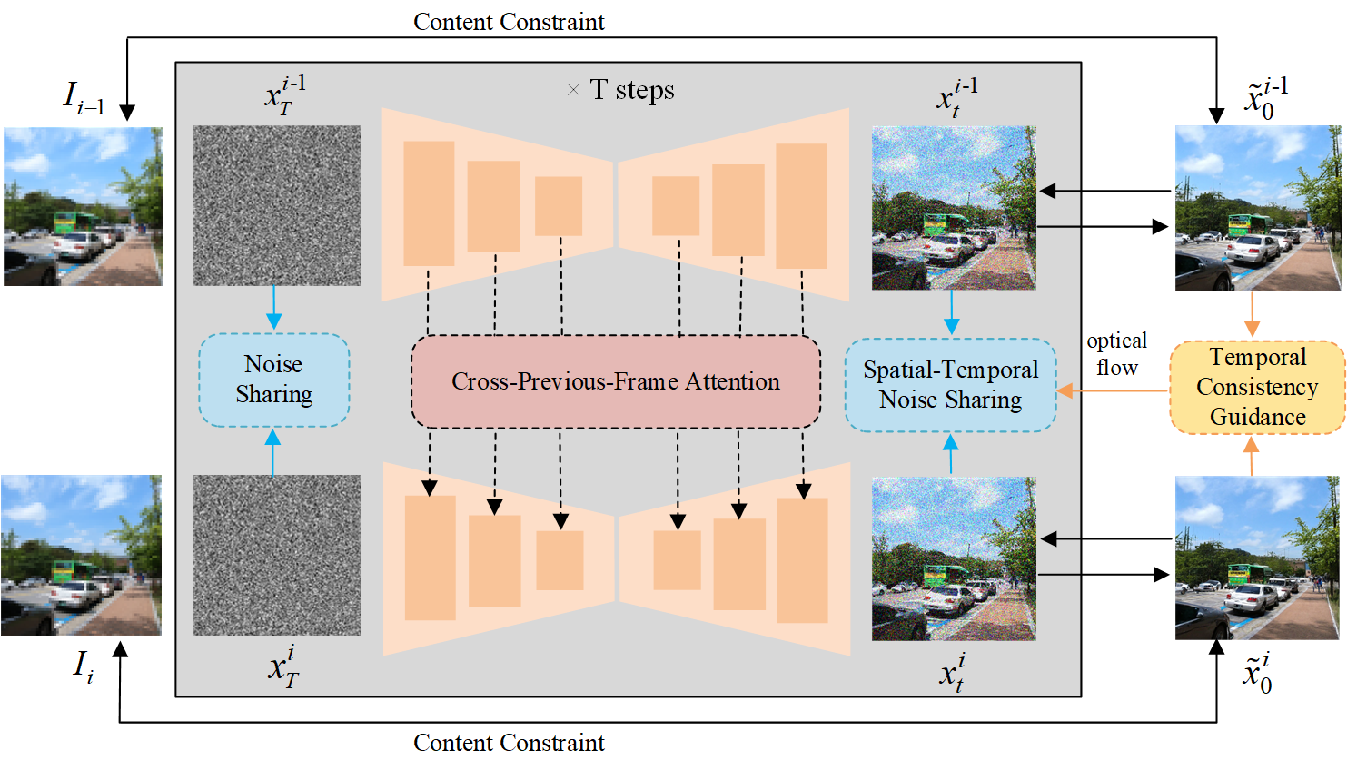
Given a degraded video with frames , our goal is to restore or enhance it to a normal-light clean video . Our method leverages a pre-trained unconditional image diffusion model [6] for video restoration and enhancement. [6] employs a U-Net which is constructed from layers of 2D convolutional residual blocks and spatial self-attention blocks. We replace all 2D convolutions with inflated 3D convolutions so that the network can process video. For better temporal consistency, we propose cross-previous-frame attention, temporal consistency guidance, spatial-temporal noise sharing, and early stopping sampling strategy, the framework is illustrated in Fig. 1 and Algo. 1 shows our whole reverse diffusion process. It’s worth noting that our method is plug-and-play, which can be inserted into any diffusion-based zero-shot image restoration or enhancement method.
4.2 Cross-Previous-Frame Attention
Similar to zero-shot video editing methods [13, 33], we replace self-attention layers in the U-Net with cross-frame attention layers to strengthen the temporal consistency between degraded frame and . For each spatial self-attention layer, the query, key, and value , , are obtained by linear projection of the feature of , the corresponding self-attention output is produced by with
| (8) |
where , , are pre-trained matrices that project the inputs to query, key and value, respectively.
Cross-frame attention uses the key and value from other frames. For zero-shot video editing, besides the previous frame, the first frame is also used to maintain the global coherence in terms of generated content. However we find that the previous frame is enough to maintain the temporal consistency between consecutive frames. To reduce the computation cost, we do not leverage more neighbor frames to compute cross-frame attention, and we find that it will not bring prominent improvement in temporal consistency. The corresponding cross-previous-frame attention output is produced by with
| (9) |
4.3 Temporal Consistency Guidance
In the sampling (reverse) process of DDPM, a clean image is usually predicted from the noisy image by estimating the noise in , which can be directly inferred when given by the Eq. 6 in every timestep . Similar to GDP [7], We can add guidance on to control the generation process of the DDPM. To achieve the better temporal consistency, we compute the optical flow and occlusion mask between the of degraded frame and , which are denoted by and . And constrain and with temporal consistency loss
| (10) |
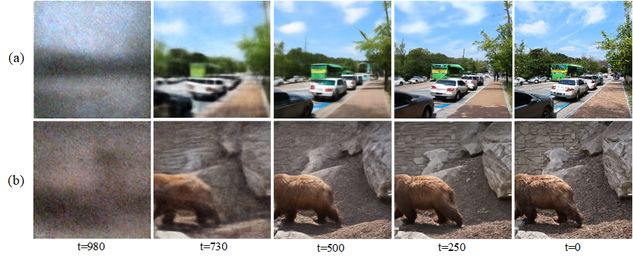
where is predicted occlusion mask, is predicted optical flow. Then we can apply gradient guidance to guide the sampling process. Specifically, we can sample by , is gradient scale. We find that the is not always clean in the whole sampling process. Like Fig 2 shows, at the beginning of sampling, has a lower signal-to-noise ratio, where the image contents are unrecognizable and has a lot of noise. In the middle part of sampling, has smooth content which can not be used to compute precise optical flow. Only in the second half of sampling, the diffusion model slowly generate rich content and details, which is suitable to compute precise optical flow. In practice, we only apply temporal consistency guidance after , is a hyper-parameter. We utilize RAFT [30, 11] as our optical flow network for temporal consistency guidance.
4.4 Spatial-Temporal Noise Sharing
Recently, [3] demonstrates that the denoising process plays an important role in the denoising diffusion model. Actually, the noise in the sampling process controls the final generated color and details. For the same degraded frame, different noise and in the sampling process will lead to different colors and details. For better temporal consistency, we propose to share the same and between all frames, which encourages the diffusion model to generate the same details in the static areas. In 4.3, we have computed the optical flow and occlusion mask between the of degraded frame and . We used the predicted optical flow and occlusion mask to blend the of degraded frame and , which are denoted by the and . We propose to blend rather than to blend , or U-Net feature since the latter usually leads to motion ghost and unpleasant artifacts. The blending process can be formulated as
| (11) |
The blending process shares noise between the corresponding pixels in different frames, which encourages the diffusion model to generate the same details in these dynamic areas.
4.5 Early Stopping Sampling Strategy
In 4.3, we find that firstly reconstructs the low-frequency component of the image, then reconstructs the high-frequency component in the sampling process, the temporal flicker easily increases at the end of the reverse diffusion process. And the real-world degraded images often suffer from noise. When enhancing low-light videos which often suffer from noise, the diffusion model will reconstruct the high-frequency noise at the end of sampling, which also reduces the temporal consistency. We propose an early stopping sampling strategy, which stops sampling after , preventing from reconstructing noise or unconsistency high-frequency details. We take the early stopping as the final result.
5 Experiments
5.1 Datasets
For evaluation of video super-resolution, we collected 18 gt videos from commonly used test datasets REDS4 [20], Vid4 [17] and UDM10 [34]. For evaluation of video inpainting, we collected 20 gt videos from the commonly used DAVIS [23] dataset. For evaluation of video colorization, we use the gt videos from Videvo20 [14] dataset, which is one of the mainly used datasets for video colorization. Due to the slow sampling speed of DDPM and a test video containing a lot of frames, we first center crop the frames along the shorter edge and then resize them to 256256, which matches the image size of the diffusion model. And our method could combine with patch-based strategy in [7] to process any-size videos. We follow [7] to apply linear degradation to gt videos to construct corresponding degraded videos for video super-resolution, inpainting, and colorization, respectively. For low-light video enhancement, we collected 10 paired low-normal videos from the DID dataset [8] which was captured in the real world. For each low and normal video, We center crop the frames along the shorter edge, and then resize them to 256256.
| Methods | PSNR | SSIM | FID | WE() |
|---|---|---|---|---|
| DDNM | 2.0976 | |||
| DDNM+ZVRD | 23.49 | 0.6904 | 107.17 | |
| GDP | 20.44 | 0.5252 | 171.59 | 5.8179 |
| GDP+ZVRD | 21.18 | 0.5722 | 174.37 | 0.4574 |
| Methods | PSNR | SSIM | FID | WE() |
|---|---|---|---|---|
| DDNM | 6.8646 | |||
| DDNM+ZVRD | 32.56 | 0.9462 | 8.4405 | |
| GDP | 26.96 | 0.8011 | 40.99 | 7.2141 |
| GDP+ZVRD | 27.05 | 0.8034 | 35.91 | 3.8836 |
| Methods | PSNR | SSIM | FID | WE() |
|---|---|---|---|---|
| DDNM | 0.9932 | 123.29 | 4.2693 | |
| DDNM+ZVRD | 25.78 | 3.2624 | ||
| GDP | 24.58 | 0.9333 | 134.56 | |
| GDP+ZVRD | 24.48 | 0.9343 | 135.64 | 2.3340 |
| Methods | PSNR | SSIM | FID | WE() |
|---|---|---|---|---|
| SGZ | 17.22 | 0.6576 | 49.49 | |
| GDP | 62.05 | 1.6011 | ||
| GDP+ZVRD | 17.51 | 0.8085 | 0.8143 |

5.2 Comparison with State-of-the-art Methods
We utilize four measurements to evaluate the restoration and enhancement quality. Besides the commonly used metrics PSNR, SSIM, and FID, we utilize Warping Error (WE) [14] to evaluate temporal consistency. Since there has been no research on zero-shot video restoration before and our method is a plug-and-play method, we choose two state-of-the-art zero-shot image restoration methods DDNM [31] and GDP [7] as our compared method and backbone. We utilize their way for the content constraint in our method and compare with them, respectively. DDNM utilizes range-null space decomposition to constrain the restored result to own the same content as the degraded image. GDP leverages distance constraints between restored/enhanced results and degraded images to guide the reverse diffusion process. GDP is based on DDPM sampling, and DDNM combines with DDIM [28] to accelerate the sampling. For the low-light video enhancement, we compared our method with the zero-shot video enhancement method SGZ [38] and the zero-shot image enhancement method GDP.
Table 1, 2, 3, 4 list the quantitative results on the evaluation data for video super-resolution, video inpainting, video colorization, and low-light video enhancement, respectively. It can be observed that by inserting our method in existing zero-shot image methods (DDNM+ZVRD, GDP+ZVRD), the temporal consistency can be obviously improved. For 4 video super-resolution, on the basis of DDNM, the WE is decreased to nearly 1/3 of the original, the PSNR, and SSIM are increased and the FID is decreased through our method. On the basis of GDP, the WE is decreased to about 1/12 of the original, and our method achieves 0.74 dB gain for PSNR, with the slightly raised FID. For 25 video inpainting, the performance is improved in all four metrics on both backbones, the WE is decreased to about half of the original on GDP. For video colorization, the WE is decreased by about 1 gain on both backbones. For low-light video enhancement, our method can boost GDP in all four metrics, and make GDP have better temporal consistency than SGZ. It demonstrates that our method is effective and can boost the performance of diffusion-based zero-shot image restoration and enhancement methods on video tasks.
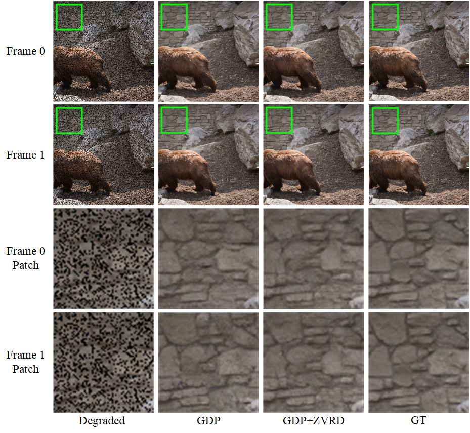
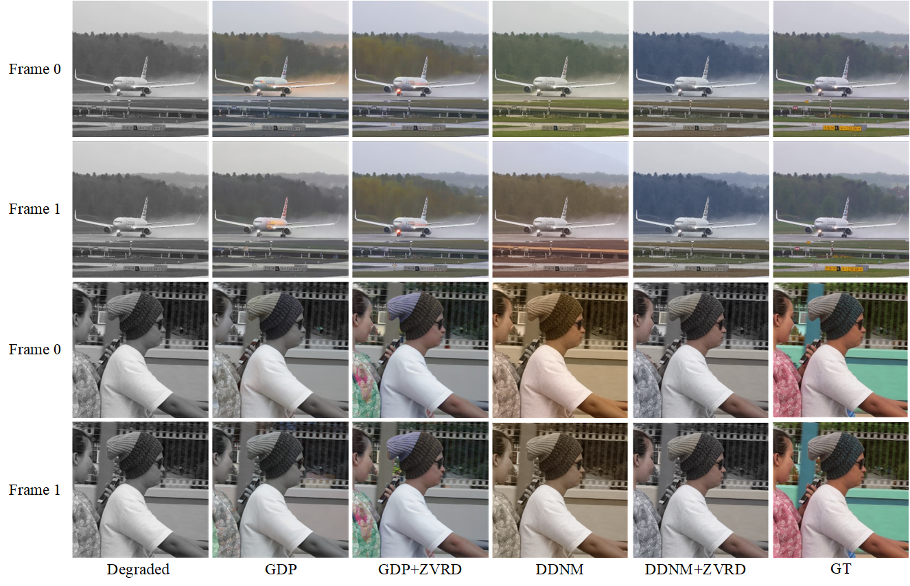
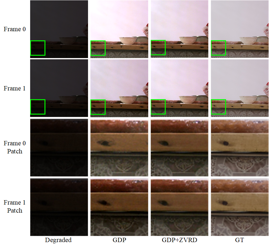
Fig. 3, 4, 5, 6 present the visual comparison results on the evaluation data for video super-resolution, video inpainting, video colorization and low-light video enhancement, respectively. Fig. 3 presents the four methods’ results on the first and second frames of the video. For GDP, the details of the tree and bus are not consistent on the two frames, and the shape of the car is also obviously different. For DDNM, there are different contents on the window of the bus. Our method (DDNM+ZVRD, GDP+ZVRD) can restore temporal consistent results on both tree and bus. Fig. 4 presents the results of GDP and GDP+ZVRD. It can be observed that the wall texture is not consistent in GDP results. Our method restores temporal consistent results which are similar to the gt frames. Fig. 5 presents the four methods’ results on two scenes. In the first scene, GDP results have different colors on the local areas of the airplane, and DDNM restores different global color styles. Compared with them, our method restores temporal consistent color in both local and global areas. In the second scene, GDP restores different colors on clothes, and the second frame of DDNM has a dimmer color than the first frame. Our method can restore more temporal consistent and colorful results. Fig. 6 presents the results on a low-light video. It can be observed that GDP has different global light and different details on the table. Our method has better temporal consistency on global light and local details.
5.3 Ablation Study
| Cross-previous-frame attention | |||||
|---|---|---|---|---|---|
| Temporal consistency guidance | |||||
| Spatial-temporal noise sharing | |||||
| Early stopping sampling strategy | |||||
| PSNR | 20.44 | 20.59 | 20.57 | 21.26 | 21.18 |
| SSIM | 0.5252 | 0.5293 | 0.5275 | 0.5790 | 0.5722 |
| FID | 171.59 | 171.64 | 172.17 | 174.33 | 174.37 |
| WE() | 5.8179 | 4.9275 | 3.0092 | 0.4746 | 0.4574 |
In this section, we perform ablation study to demonstrate the effectiveness of the proposed cross-previous-frame attention, temporal consistency guidance, spatial-temporal noise sharing and early stopping sampling strategy. Take video super-resolution as an example, Table 5 lists the quantitative comparison results in evaluation data by adding these modules one by one. It can be observed that the WE is decreased by nearly 1 gain when adding cross-previous-frame attention, nearly 2 gain when adding temporal consistency guidance, decreased by 5/6 when adding spatial-temporal noise sharing, and slightly decreased when adding early stopping sampling strategy. The four modules all bring slightly worse FID, but are acceptable according to the visual comparison results in 5.2. Cross-previous-frame attention and spatial-temporal noise sharing are beneficial to fidelity, especially the latter, which brings 0.69 dB gain for PSNR.
6 Conclusion
In this paper, we propose the first framework for zero-shot video restoration and enhancement which uses a pretrained image diffusion model and is training-free. By replacing the self-attention layer with the proposed cross-previous-frame attention layer, the pre-trained image diffusion model can utilize the temporal correlation between frames, which is beneficial to temporal consistency. To further strengthen the temporal consistency of results, we propose temporal consistency guidance, spatial-temporal noise sharing, and an early stopping sampling strategy. Our method can be inserted into any diffusion-based zero-shot image restoration or enhancement method. Experimental results demonstrate the superiority of the proposed method in producing temporally consistent videos with better fidelity.
References
- [1] Ceylan, D., Huang, C.H.P., Mitra, N.J.: Pix2video: Video editing using image diffusion. In: Proceedings of the IEEE/CVF International Conference on Computer Vision. pp. 23206–23217 (2023)
- [2] Chai, W., Guo, X., Wang, G., Lu, Y.: Stablevideo: Text-driven consistency-aware diffusion video editing. arXiv preprint arXiv:2308.09592 (2023)
- [3] Chen, X., Liu, Z., Xie, S., He, K.: Deconstructing denoising diffusion models for self-supervised learning. arXiv preprint arXiv:2401.14404 (2024)
- [4] Choi, J., Kim, S., Jeong, Y., Gwon, Y., Yoon, S.: Ilvr: Conditioning method for denoising diffusion probabilistic models. In: Proceedings of the IEEE/CVF International Conference on Computer Vision (ICCV) (2021)
- [5] Chung, H., Kim, J., Mccann, M.T., Klasky, M.L., Ye, J.C.: Diffusion posterior sampling for general noisy inverse problems. arXiv preprint arXiv:2209.14687 (2022)
- [6] Dhariwal, P., Nichol, A.: Diffusion models beat gans on image synthesis. Advances in neural information processing systems 34, 8780–8794 (2021)
- [7] Fei, B., Lyu, Z., Pan, L., Zhang, J., Yang, W., Luo, T., Zhang, B., Dai, B.: Generative diffusion prior for unified image restoration and enhancement. In: Proceedings of the IEEE/CVF Conference on Computer Vision and Pattern Recognition. pp. 9935–9946 (2023)
- [8] Fu, H., Zheng, W., Wang, X., Wang, J., Zhang, H., Ma, H.: Dancing in the dark: A benchmark towards general low-light video enhancement. In: Proceedings of the IEEE/CVF International Conference on Computer Vision. pp. 12877–12886 (2023)
- [9] Hertz, A., Mokady, R., Tenenbaum, J., Aberman, K., Pritch, Y., Cohen-Or, D.: Prompt-to-prompt image editing with cross attention control. arXiv preprint arXiv:2208.01626 (2022)
- [10] Ho, J., Jain, A., Abbeel, P.: Denoising diffusion probabilistic models. Advances in neural information processing systems 33, 6840–6851 (2020)
- [11] Jeong, H., Ye, J.C.: Ground-a-video: Zero-shot grounded video editing using text-to-image diffusion models. arXiv preprint arXiv:2310.01107 (2023)
- [12] Kawar, B., Elad, M., Ermon, S., Song, J.: Denoising diffusion restoration models. In: ICLR Workshop on Deep Generative Models for Highly Structured Data (ICLRW) (2022)
- [13] Khachatryan, L., Movsisyan, A., Tadevosyan, V., Henschel, R., Wang, Z., Navasardyan, S., Shi, H.: Text2video-zero: Text-to-image diffusion models are zero-shot video generators. arXiv preprint arXiv:2303.13439 (2023)
- [14] Lai, W.S., Huang, J.B., Wang, O., Shechtman, E., Yumer, E., Yang, M.H.: Learning blind video temporal consistency. In: Proceedings of the European conference on computer vision (ECCV). pp. 170–185 (2018)
- [15] Li, J., Liang, Q., Li, Q., Gang, R., Fang, J., Lin, C., Feng, S., Liu, X.: Rttlc: Video colorization with restored transformer and test-time local converter. In: Proceedings of the IEEE/CVF Conference on Computer Vision and Pattern Recognition. pp. 1722–1730 (2023)
- [16] Liang, J., Cao, J., Fan, Y., Zhang, K., Ranjan, R., Li, Y., Timofte, R., Van Gool, L.: Vrt: A video restoration transformer. arXiv preprint arXiv:2201.12288 (2022)
- [17] Liu, C., Sun, D.: On bayesian adaptive video super resolution. IEEE transactions on pattern analysis and machine intelligence 36(2), 346–360 (2013)
- [18] Lugmayr, A., Danelljan, M., Romero, A., Yu, F., Timofte, R., Van Gool, L.: Repaint: Inpainting using denoising diffusion probabilistic models. In: Proceedings of the IEEE/CVF Conference on Computer Vision and Pattern Recognition (CVPR) (2022)
- [19] Mansour, Y., Heckel, R.: Zero-shot noise2noise: Efficient image denoising without any data. In: Proceedings of the IEEE/CVF Conference on Computer Vision and Pattern Recognition. pp. 14018–14027 (2023)
- [20] Nah, S., Baik, S., Hong, S., Moon, G., Son, S., Timofte, R., Mu Lee, K.: Ntire 2019 challenge on video deblurring and super-resolution: Dataset and study. In: Proceedings of the IEEE/CVF Conference on Computer Vision and Pattern Recognition Workshops. pp. 0–0 (2019)
- [21] Nichol, A.Q., Dhariwal, P.: Improved denoising diffusion probabilistic models. In: International Conference on Machine Learning. pp. 8162–8171. PMLR (2021)
- [22] Ouyang, H., Wang, Q., Xiao, Y., Bai, Q., Zhang, J., Zheng, K., Zhou, X., Chen, Q., Shen, Y.: Codef: Content deformation fields for temporally consistent video processing. arXiv preprint arXiv:2308.07926 (2023)
- [23] Pont-Tuset, J., Perazzi, F., Caelles, S., Arbeláez, P., Sorkine-Hornung, A., Van Gool, L.: The 2017 davis challenge on video object segmentation. arXiv preprint arXiv:1704.00675 (2017)
- [24] Qi, C., Cun, X., Zhang, Y., Lei, C., Wang, X., Shan, Y., Chen, Q.: Fatezero: Fusing attentions for zero-shot text-based video editing. arXiv preprint arXiv:2303.09535 (2023)
- [25] Rombach, R., Blattmann, A., Lorenz, D., Esser, P., Ommer, B.: High-resolution image synthesis with latent diffusion models. In: Proceedings of the IEEE/CVF conference on computer vision and pattern recognition. pp. 10684–10695 (2022)
- [26] Saharia, C., Ho, J., Chan, W., Salimans, T., Fleet, D.J., Norouzi, M.: Image super-resolution via iterative refinement. IEEE Transactions on Pattern Analysis and Machine Intelligence 45(4), 4713–4726 (2022)
- [27] Shi, Z., Liu, R.: Conditional velocity score estimation for image restoration. In: Proceedings of the IEEE/CVF Winter Conference on Applications of Computer Vision. pp. 179–188 (2024)
- [28] Song, J., Meng, C., Ermon, S.: Denoising diffusion implicit models. arXiv preprint arXiv:2010.02502 (2020)
- [29] Song, Y., Ermon, S.: Generative modeling by estimating gradients of the data distribution. Advances in Neural Information Processing Systems (NeurIPS) 32 (2019)
- [30] Teed, Z., Deng, J.: Raft: Recurrent all-pairs field transforms for optical flow. In: Computer Vision–ECCV 2020: 16th European Conference, Glasgow, UK, August 23–28, 2020, Proceedings, Part II 16. pp. 402–419. Springer (2020)
- [31] Wang, Y., Yu, J., Zhang, J.: Zero-shot image restoration using denoising diffusion null-space model. arXiv preprint arXiv:2212.00490 (2022)
- [32] Wu, J.Z., Ge, Y., Wang, X., Lei, S.W., Gu, Y., Shi, Y., Hsu, W., Shan, Y., Qie, X., Shou, M.Z.: Tune-a-video: One-shot tuning of image diffusion models for text-to-video generation. In: Proceedings of the IEEE/CVF International Conference on Computer Vision. pp. 7623–7633 (2023)
- [33] Yang, S., Zhou, Y., Liu, Z., Loy, C.C.: Rerender a video: Zero-shot text-guided video-to-video translation. arXiv preprint arXiv:2306.07954 (2023)
- [34] Yi, P., Wang, Z., Jiang, K., Jiang, J., Ma, J.: Progressive fusion video super-resolution network via exploiting non-local spatio-temporal correlations. In: Proceedings of the IEEE/CVF international conference on computer vision. pp. 3106–3115 (2019)
- [35] Yin, Y., Xu, D., Tan, C., Liu, P., Zhao, Y., Wei, Y.: Cle diffusion: Controllable light enhancement diffusion model. In: Proceedings of the 31st ACM International Conference on Multimedia. pp. 8145–8156 (2023)
- [36] Zhang, Y., Wei, Y., Jiang, D., Zhang, X., Zuo, W., Tian, Q.: Controlvideo: Training-free controllable text-to-video generation. arXiv preprint arXiv:2305.13077 (2023)
- [37] Zhao, M., Wang, R., Bao, F., Li, C., Zhu, J.: Controlvideo: Adding conditional control for one shot text-to-video editing. arXiv preprint arXiv:2305.17098 (2023)
- [38] Zheng, S., Gupta, G.: Semantic-guided zero-shot learning for low-light image/video enhancement. In: Proceedings of the IEEE/CVF Winter conference on applications of computer vision. pp. 581–590 (2022)
- [39] Zhou, S., Li, C., Chan, K.C., Loy, C.C.: Propainter: Improving propagation and transformer for video inpainting. In: Proceedings of the IEEE/CVF International Conference on Computer Vision. pp. 10477–10486 (2023)
Zero-shot Video Restoration and Enhancement Using Pre-Trained Image Diffusion Model
– Supplementary Material –
Cong Cao, Huanjing Yue, Xin Liu, and Jingyu Yang
This supplementary file provides additional details that were not included in the main paper due to page limitations. In the following, we first give the detailed experiment settings, and then present comparison results on video deblurring and denoising. Finally, a demo for video results comparison is given.
| Methods | PSNR | SSIM | FID | WE() |
|---|---|---|---|---|
| DPS | 20.92 | 0.6206 | 205.19 | 6.7240 |
| DPS+ZVRD | 21.54 | 0.6307 | 202.26 | 2.3519 |
| Methods | PSNR | SSIM | FID | WE() |
|---|---|---|---|---|
| ZS-N2N | 25.33 | 0.6749 | 267.98 | 7.0208 |
| DDNM | 0.8285 | 136.73 | ||
| DDNM+ZVRD | 28.11 | 5.9865 |
7 Experiment Settings
The evaluation datasets for video super-resolution, video inpainting, video colorization, and low-light video enhancement are mentioned in the main file. For the three restoration tasks, we follow the settings of the linear degradation operator from [31, 7]. For super-resolution with , we set the degradation operator as the average-pooling operator , which averages each patch into a single value. For inpainting, the degradation operator is the mask operator. For colorization, the degradation operator is a pixel-wise operator that converts each RGB channel pixel into a grayscale value. In addition to the aforementioned four tasks, we further compare our method in two restoration tasks: video deblurring and video denoising. For video deblurring, we collected 10 gt videos from the dataset REDS [20], and center crop the frames with resolution 256256. Then we add motion blur on gt videos to construct the degraded videos, the blur kernels are 3333 with a strength of 0.5. For video denoising, we collected 15 gt videos from the commonly used test dataset Set8 [tassano2020fastdvdnet] and DAVIS [23]. For each video, We center-crop the frames along the shorter edge, and then resize them to 256256. We add Gaussian noise with on gt videos to construct the noisy videos. The sampling hyper-parameters and are set to 300 and 0.5, respectively. The early stopping sampling strategy is only applied to video super-resolution, inpainting and low-light video enhancement, the hyper-parameter is set to 50.
8 Comparison on More Tasks
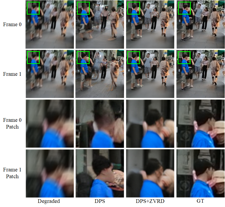
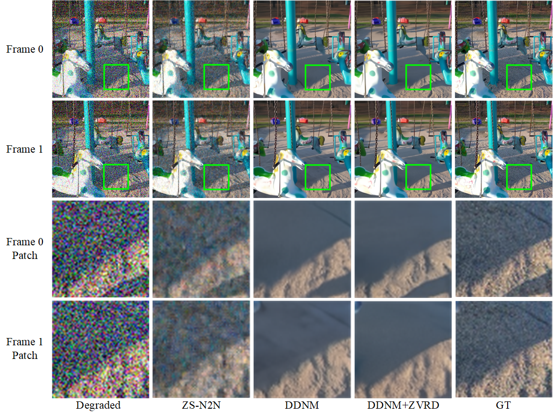
For video deblurring and denoising, we choose DPS [5] and DDNM [31] as our compared method and backbone, respectively. And we compare with a zero-shot image denoising method ZS-N2N [19] on noisy videos. Table 6, 7 list the quantitative results of the evaluation data for video deblurring and denoising, respectively. It can be observed that by inserting our method in two image methods (DPS+ZVRD, DDNM+ZVRD), the temporal consistency can be improved. Especially when applied to video deblurring, our method boosts the performance of all four metrics, the WE is decreased to nearly 1/3 of the original.
Fig. 7, 8 present the visual comparison results on the evaluation data for video deblurring and denoising, respectively. Fig. 7 presents the results of DPS and DPS+ZVRD. It can be observed that the human body is not consistent in DPS results. Our method restores temporal consistent results which are more similar to the gt frames. Fig. 8 presents the results of three methods on the first and second frames. The results of ZS-N2N still remain noise, which also reduces the temporal consistency. Compared with DDNM, our method restores more temporally consistent results in sand areas. We also present a video demo to further present the temporal consistency of our method.
