FlowTrack: Point-level Flow Network for 3D Single Object Tracking
Abstract
3D single object tracking (SOT) is a crucial task in fields of mobile robotics and autonomous driving. Traditional motion-based approaches achieve target tracking by estimating the relative movement of target between two consecutive frames. However, they usually overlook local motion information of the target and fail to exploit historical frame information effectively. To overcome the above limitations, we propose a point-level flow method with multi-frame information for 3D SOT task, called FlowTrack. Specifically, by estimating the flow for each point in the target, our method could capture the local motion details of target, thereby improving the tracking performance. At the same time, to handle scenes with sparse points, we present a learnable target feature as the bridge to efficiently integrate target information from past frames. Moreover, we design a novel Instance Flow Head to transform dense point-level flow into instance-level motion, effectively aggregating local motion information to obtain global target motion. Finally, our method achieves competitive performance with improvements of 5.9% on the KITTI dataset and 2.9% on NuScenes. The code will be made publicly available soon.
I Introduction
3D single object tracking, an essential task in 3D computer vision, plays a crucial role in the fields of mobile robotics and autonomous driving. Given an initial target state, 3D SOT aims to capture the state of the target in subsequent frames, which can provide real-time information of target for downstream tasks like path planning and decision-making.
Inspired by 2D image tracking [1, 2, 3], the previous 3D SOT methods [4, 5, 6] usually treat object tracking as a matching problem. They utilize siamese networks to extract features from the template and the current frame, then rely on appearance matching to locate the target in the current frame. However, in scenes with object occlusion, interference from similar objects and distant target tracking, these matching-based methods face challenges due to the sparsity and disorder of point clouds.
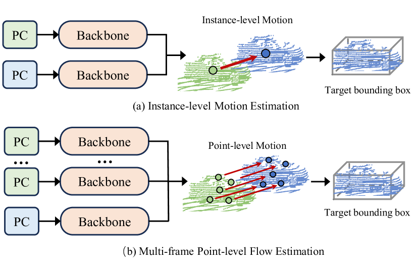
Unlike the matching-based methods, some methods [7, 8] regard the tracking task as motion prediction and locate the target by predicting the relative motion between two adjacent frames. This motion-based paradigm alleviates the difficulty faced by appearance matching in the above challenge scenarios. However, these methods only focus on instance-level target motion and ignore the local motion details of the target. Additionally, they only utilize short-term motion cues between two frames, disregarding long-term geometry and motion information of the target from historical frames.
To address the above problems, we introduce the idea of optical flow estimation [9, 10] and propose a multi-frame point-level flow network, named FlowTrack. As shown in Fig. 1, unlike traditional motion-based methods, our proposed network can effectively capture the local motion details of the target by predicting the motion of each feature point in the target. Meanwhile, the rich geometric and motion information contained in historical frames offers valuable information supplements for estimating target motion, especially in scenes with sparse point clouds.
Specifically, FlowTrack first extracts BEV features of consecutive frame point clouds by 3D sparse convolution [11]. Then, to extract rich motion and geometry information of the target in historical frames, we propose a Historical Information Fusion Module (HIM) to efficiently fuse the information of target from historical frames into the template frame. Subsequently, we concatenate the template and current features along the channel as flow feature and use a proposed Point-level Motion Module (PMM) to extract multi-scale point-level flow feature of target. Finally, with the aid of the Instance Flow head (IFH), our method accurately transform the point-level flow of the target into instance-level motion, achieving precise relative motion estimation of the target. Extensive experiments have demonstrated that our method achieves superior tracking performance than existing motion-based methods.
The main contributions of this paper are as follows:
-
•
We propose a multi-frame point-level flow tracking framework to achieve effective capture of the target motion information.
-
•
We design HIM, PMM, and IFH to achieve historical information fusion, target point-level flow estimation, and instance-level motion prediction respectively.
-
•
Our approach achieves competitive performance on the KITTI and nuScenes datasets. Extensive ablation studies demonstrate the effectiveness of the proposed modules.
II Related Work
II-A 3D Single Object Tracking
Early 3D SOT methods [4, 5, 12] regard target tracking as a matching issue. They use the Siamese network to extract features of two consecutive frames and employ similarity matching for target localization. SC3D [4] is the first method to introduce the Siamese network structure into 3D SOT, enabling the capture of the target shape and subsequent generation of a series of bounding boxes within the search area. P2B [5] calculates point-level cosine similarity maps to enhance search features and adopts VoteNet [13] for end-to-end prediction of the bounding box for target. PTTR [14] and STNet [6] utilize the Transformer-based structure [15] to promote intra-frame information exchange and inter-frame target association. STTracker [16] goes a step further by incorporating multi-frame information to improve the performance of matching approaches. Although the match-based paradigm has been successful in 3D SOT, it overlooks the motion information of the target. Additionally, the sparsity and occlusion of point clouds also pose significant challenges to appearance matching.
To alleviate this problem, M2-Track [7] proposes a motion-based approach, modeling the target’s relative motion instead of locating target through appearance-matching in two consecutive frames. DMT [8] designs a motion prediction module, which estimates the potential center of the target based on historical bounding boxes, and then refines it using a voting module. However, these methods only consider instance-level motion of target and overlook the local motion details of the target. Besides, they do not effectively utilize the rich structural and motion information in historical frame point clouds.
II-B Optical Flow Estimation
Initially, the optical flow estimation is modeled as an optimization problem, aiming to maximize the visual similarity between image pairs with the regularizations [17, 18]. The advent of deep learning networks has significantly promoted advancements in this field. FlowNet [19] is the first end-to-end convolutional neural network for optical flow estimation, but it faces challenge to handle large object displacement motions. Afterward, RAFT [9] uses loop iteration at multiple scales to achieve excellent performance with the cost of increased processing time. GMFlow [10] further improves the accuracy and efficiency of optical flow estimation by combining similarity matching and global attention through convolution networks. Furthermore, FlowFormer [20] represents the pioneering method that deeply integrates transformers with cost volumes for optical flow estimation. Inspired by the above methods, we integrate the concept of optical flow into the 3D SOT. By estimating point-level flow of the target, our network captures detailed local motion information of the target, thus achieving more accurate and robust tracking.

III METHODOLOGY
III-A Framework Overview
Given a initial bounding box , the 3D SOT task aims to estimate the in the subsequent frame. Here, , , and demote the 3D center, size and orientation, respectively. Moreover, the size of target is assumed to remain unchanged [5], thus we solely require to estimate the target center and orientation . For motion-based paradigm, given two consecutive frames and (termed as current and template frames) and target 3D bounding box in frame, the tracker is required to predict the relative instance-level movement between the two adjacent frames, i.e. the translation offsets () and rotation angle . Then, a rigid body transformation is applied to obtain the target bounding box in the current frame. This process could be expressed as follows:
| (1) |
| (2) |
Unlike the traditional motion-based approach, we replace the coarse relative instance-level motion by estimating the fine-grained relative point-level flow for the target, while incorporating historical frame information. Subsequently, through a proposed Instance Flow Head, we efficiently convert point-level flow into relative instance-level motion and derive for the current frame utilizing a rigid body transformation. Thus, our point-level flow paradigm could be formulated as follows:
| (3) |
| (4) |
where is the relative point-level from frame to the current frame.
Based on Eq. 3 and Eq. 4, we propose a multi-frame point-level flow network, which performs SOT by estimating the relative point-level flow of the target. As displayed in Fig. 2, given the point clouds from historical and current frames, we first extract BEV features for each frame. Afterward, we design a Historical Information Fusion Module to efficiently integrate target features from historical features, which supplements the geometric and motion information of the target. Then, we concatenate the template and current features as flow feature and feed it into the Point-level Motion Module to capture local motion details of the target at multiple scales. Finally, the proposed Instance Flow Head predicts the point-level flow of the target and converts it into instance-level relative motion of the target, achieving target tracking through rigid body transformation.
III-B Historical Information Fusion
Traditional motion-based algorithm [7] only utilizes two consecutive frames, overlooking the rich spatial and motion information of target in history frames. To extract target information in historical frames, we introduce a Historical Information Fusion Module based on a learnable target feature. It uses the learnable target feature as a bridge and employs Transformer [21] to achieve inter-frame target feature interaction, while reducing interference from background information in historical frames.
Following previous methods [22], we initially extract voxel features by voxelizing each frame’s point cloud and employing three layers of 3D sparse convolution. Then, we compress the height dimension of the voxel features from the final layer to generate multi-frame BEV features . Additionally, to highlight the target feature in the template feature, we define a template box mask , where the mask value is set to 1 for grid points whose center lies within the box and 0 for others, as expressed in Eq. 5.
Learnable Target Feature Initialization. Based on the number of feature points occupied by the target in the template feature , we initially define a learnable target feature . Here, and denote the number of feature points in the target and the channel. As shown in Fig. 3(a), we update it with the target feature in the template frame by cross-attention. Specifically, we first concatenate with along the feature channels and pass it through a 2D convolution layer to obtain mask-enhanced . Then, we use cross-attention to fuse the target information from into , achieving the update of . By using as guidance, we ensure learns target information rather than background information. This process can be expressed by the following formula:
| (5) |
| (6) |
| (7) |
Here, and denote the updated learnable target feature and concatenation operation, while CA and SA stand for Cross-Attention and Self-Attention.
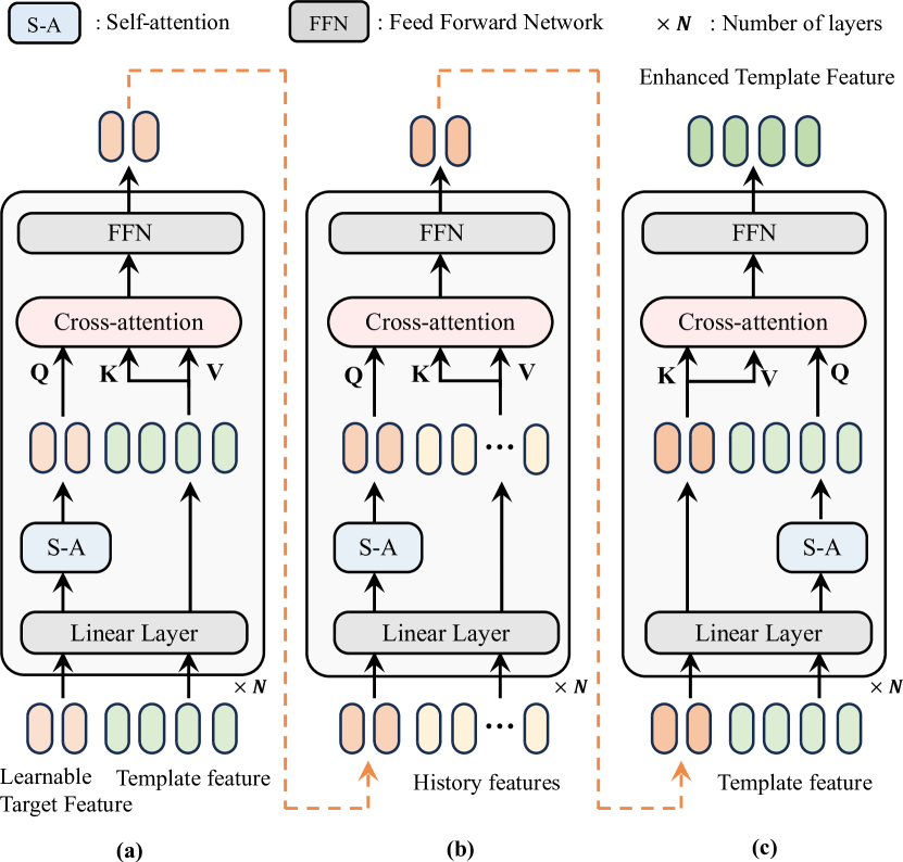
Target Feature Interaction. As shown in Fig. 3(b),(c), by using the updated as bridge, the model can interact and complement the information of the target feature in the history frames, eventually enhancing the target feature in the template frame. Similar to Eq. 7, we aggregate the target information from historical frames into and then use the enhanced feature to enrich the template feature . Specifically, using as the query, history features as key and value, we get the enhanced target feature by cross-attention, as shown in Fig. 3(b). Thus, contains geometric and motion information of historical target. Finally, using as the query, as the key and value, we integrate historical target information into the and get the enhanced template feature , as shown in Fig. 3(c).
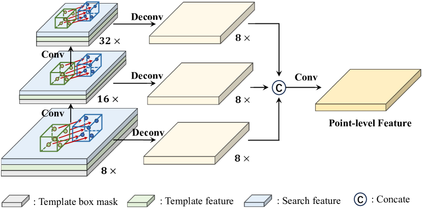
III-C Point-level Motion Module
Unlike motion-based methods that directly predict the instance-level motion of target, we capture local motion details within the target by predicting point-level flow, thereby achieving fine-grained motion estimation. However, different classes and sizes of tracked targets have different scales of motion. To fully capture their motion information, it is crucial to obtain point-level flow feature of the targets at multiple scales, as shown in Fig. 4.
To obtain the initial point-level flow feature , we first concatenate the template box mask , the enhanced template feature and the current feature along the channel. Then, we use three layers of 2D convolution for downsampling to extract multi-scale point-level flow features , where represents the label of the scale. Lastly, we upsample each feature in to the size of the input feature and concatenate them along the channel to obtain final point-level flow feature . The above process can be represented by the following procedure:
| (8) |
| (9) |
| (10) |
Here, represents a 3-layer convolution block, which performs three downsampling operations on the input . In Eq. 9, is a collection of features from each convolutional layer output.
To train the Point-level Motion Module, we need to get point-level flow ground truth, denoted as . Initially, we project the point cloud and target bounding box of frame to frame to eliminate vehicle self-motion. Meanwhile, we define the center point position and orientation angle of the target in these two frames as (), (). Next, to obtain the ground truth , we need to calculate the coordinate maps , in and frames, where means the coordinates of each point on the feature map along the x-axis and y-axis. can be easily obtained using the target bounding box , while is computed by transforming through translation and rotation, aiming to maintain the correspondence of target feature points across frames. Finally, we calculate by subtracting the value of and . This process can be expressed by the following formula:
| (11) |
| (12) |
| (13) |
Here, and represent the translation and rotation of the target, respectively. represents the transformation from orientation angle to rotation matrix.
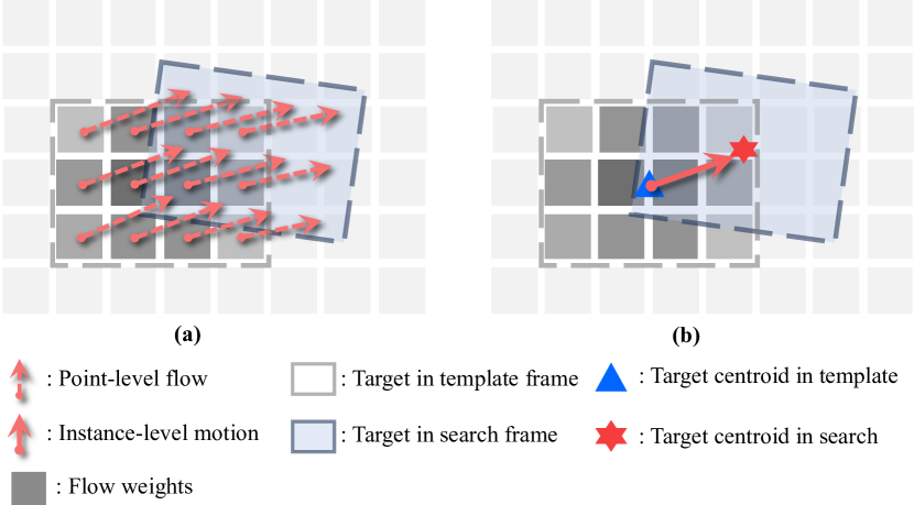
III-D Instance Flow Head
To predict the point-level flow of the target and convert it into instance-level motion, we introduce the Instance Flow Head (IFH). It predicts the point-level flow map and the flow weight map . Here, represents the relative motion of each point of the target on the feature map, while denotes the weight of each point towards the overall motion. Specifically, using the input point-level flow feature , the IFH employs two separate convolutional layers to predict and . As shown in Fig. 5, the final instance-level target motion is calculated by weighted averaging the value in using . The formula for this process is expressed as follows:
| (14) |
Here, and represent coordinates on the feature map.
Through the prediction of , the network can dynamically learn the motion weights of various points within the target, effectively distinguishing between foreground and background points. Then, we obtain the position coordinates of the target box along the x-axis and y-axis following Eq. 4. For the z-axis location coordinate and the orientation of the target, we directly predict them by two independent convolution layers.
| Method | Paradigm | Source | Car | Ped. | Van | Cyc. | Mean | |
| 6,424 | 6,088 | 1,248 | 308 | 14,068 | ||||
| Success / Precision | P2B [5] | Match | CVPR 2020 | 56.2/72.8 | 28.7/49.6 | 40.8/48.4 | 32.1/44.7 | 42.4/60.0 |
| PTT [23] | IROS 2021 | 67.8/81.8 | 44.9/72.0 | 43.6/52.5 | 37.2/47.3 | 55.1/74.2 | ||
| BAT [24] | ICCV 2021 | 60.5/77.7 | 42.1/70.1 | 52.4/67.0 | 33.7/45.4 | 51.2/72.8 | ||
| PTTR [14] | CVPR 2022 | 65.2/77.4 | 50.9/81.6 | 52.5/61.8 | 65.1/90.5 | 57.9/78.1 | ||
| SMAT [25] | RAL 2022 | 71.9/82.4 | 52.1/81.5 | 41.4/53.2 | 61.2/87.3 | 60.4/79.5 | ||
| STNet [6] | ECCV 2022 | 72.1/84.0 | 49.9/77.2 | 58.0/70.6 | 73.5/93.7 | 61.3/80.1 | ||
| GLT-T [26] | AAAI 2023 | 68.2/82.1 | 52.4/78.8 | 52.6/62.9 | 68.9/92.1 | 60.1/79.3 | ||
| CAT [27] | TNNLS 2023 | 66.6/81.8 | 51.6/77.7 | 53.1/69.8 | 67.0/90.1 | 58.9/79.1 | ||
| STTracker [16] | RAL 2023 | 66.5/79.9 | 60.4/89.4 | 50.5/63.6 | 75.3/93.9 | 62.6/82.9 | ||
| M2-Track [7] | Motion | CVPR 2022 | 65.5/80.8 | 61.5/88.2 | 53.8/70.7 | 73.2/93.5 | 62.9/83.4 | |
| DMT [8] | T-ITS 2023 | 66.4/79.4 | 48.1/77.9 | 53.3/65.6 | 70.4/92.6 | 55.1/75.8 | ||
| Ours | - | 74.8/84.4 | 65.0/92.5 | 54.3/65.3 | 79.1/94.7 | 68.8/86.4 | ||
| Improvement | - | - | 2.7/0.4 | 3.5/3.1 | 3.7/5.4 | 3.8/0.8 | 5.9/3.0 |
III-E Training Loss
We adopt a similar approach to CenterPoint [28] for predicting the target’s relative motion along the x-axis and y-axis, z-axis position and orientation. Specifically, we predict the relative point-level flow map (), flow weight map (), z-axis location map () and orientation map () with an 8 downsampling. Following Eq. 14, the target’s relative motion can be obtained from and . Additionally, we assume that points within the target box have the same z-axis position and orientation. Thus, the head loss can be defined as follows:
| (15) |
Here, we use L1 loss for , , and for attribute regression. , , and are the weights for these losses respectively. To balance the network’s consideration between point-level flow and flow weight map, we set the weight ratio of to as 1:2.
IV EXPERIMENTS
IV-A Experimental Settings
Datasets & Evaluation. We train and evaluate our method on KITTI dataset [29] and nuScenes dataset [30]. KITTI dataset includes over 20,000 3D objects tracked in 21 scenes. nuScenes dataset comprises a total of 1,000 scenes, with each frame containing approximately 300,000 points. We follow the One Pass Evaluation (OPE) protocol [31] for model evaluation, which comprises two metrics: Success and Precision. Success quantifies the degree of overlap between predicted and ground truth bounding boxes, while Precision indicates the localization accuracy of the target.
Implementation Details. We utilize sparse 3D convolution [22] widely used in 3D detection as our 3D feature extraction backbone. For our attention-based HIF Module, we follow common settings in Vision Transformer [32] with the number of heads set to 8 and the number of layers set to 6. During training, we employ the Adam optimizer with an initial learning rate of 0.0003 and weight decay of 0.01 for both datasets. Training consists of 80 epochs on KITTI and 40 epochs on nuScenes, utilizing 2 NVIDIA 4090 GPUs. We set a batch size of 64 per GPU during the training phase.
| Method | Paradigm | Car | Ped. | Trailer | Bic. | Mean | |
| 64,159 | 33,227 | 3,352 | 2,292 | 103,030 | |||
| Success | PTT [23] | Match | 41.22 | 19.33 | 50.23 | 28.39 | 35.52 |
| P2B [5] | 38.81 | 28.39 | 48.96 | 26.32 | 35.50 | ||
| BAT [24] | 40.73 | 28.83 | 52.59 | 27.17 | 39.98 | ||
| SMAT [25] | 43.51 | 32.27 | 37.45 | 25.74 | 39.29 | ||
| PTTR [23] | 51.89 | 29.90 | 45.87 | - | 44.44 | ||
| STTracker [16] | 56.11 | 37.58 | 48.13 | 36.23 | 49.43 | ||
| M2-Track [7] | Motion | 55.85 | 32.10 | 57.61 | 36.32 | 47.81 | |
| Ours | 60.29 | 37.60 | 55.39 | 43.74 | 52.35 | ||
| Improvement | - | 4.18 | 0.02 | 2.21 | 7.42 | 2.92 | |
| Precision | PTT [23] | Match | 45.26 | 32.03 | 48.56 | 51.19 | 41.89 |
| P2B [5] | 43.18 | 52.24 | 40.05 | 47.80 | 46.10 | ||
| BAT [24] | 43.29 | 53.32 | 44.89 | 51.37 | 46.76 | ||
| SMAT [25] | 49.04 | 60.28 | 34.10 | 61.06 | 52.45 | ||
| PTTR [23] | 58.61 | 45.09 | 38.36 | - | 53.48 | ||
| STTracker [16] | 69.07 | 68.36 | 55.40 | 71.62 | 68.55 | ||
| M2-Track [7] | Motion | 65.09 | 60.92 | 58.26 | 67.50 | 66.77 | |
| Ours | 71.07 | 67.64 | 62.70 | 71.43 | 69.70 | ||
| Improvement | - | 2.00 | 0.71 | 4.44 | 0.19 | 1.15 |
IV-B Quantitative Results
Results on KITTI. As shown in Tab. I, our method outperforms the best matching-based paradigm, STTracker [16], by 6.2%/3.5% in Success/Precision and surpasses the best motion-based paradigm, M2-Track [7], by 5.9%/3.0% in Success/Precision. Specifically, Pedestrian targets typically present sparser point clouds and are more susceptible to interference from similar pedestrians. This poses challenges for appearance-based matching methods [6, 24, 14]. M2-Track [7] partially addresses this challenge by predicting instance-level relative motion for tracking task. However, It overlooks the local motion details of the target and prior information from historical frames, resulting in suboptimal performance. Our method further transforms tracking task into a point-level flow estimation task, which effectively captures the local motion details of target, thereby improving the tracking performance in similar interference scenes. Meanwhile, in sparse tracking scenes, our method leverages the target information from multiple historical frames, resulting in a performance enhancement of 4.6%/3.1% in Success/Precision for the pedestrian category.
Results on nuScenes. We validated our method on the larger tracking dataset nuScenes, and the result is shown in Tab. II. Our method surpasses the best motion-based method[7] by 4.54%/6.12% in Success/Precision and outperforms the best match-based method [16] by 2.92%/1.15% in Success/Precision. In particular, for the largest number of categories, vehicle, our method achieves outstanding performance improvements, outperforming the suboptimal method by 4.18%/2.00% in Success/Precision. This is mainly attributed to the accurate capture of vehicle local motion details by the PMM module and the effective aggregation of historical information by the HIM module. Meanwhile, we observe that our model does not demonstrate superior performance when tracking large-size targets, such as Vans in KITTI and Trailers in nuScenes. We believe that the larger size of these targets results in significant variations in local point motion, thereby affecting the final instance-level motion estimation.
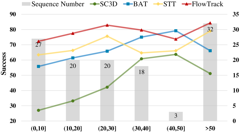
Robustness to Sparseness. In Fig. 6, consistent with prior studies [4, 24, 16], we display tracking performance under the different number of points for the target in the initial frame. our method surpasses alternative approaches in the majority of scenarios, specifically those with fewer than 40 points. This result confirms the distinct advantage of our method when dealing with sparse scenarios.
Running speed. As shown in Tab. III, despite the introduction of multiple frames in our method, we still maintain a decent inference speed of 33.2 FPS for the model.
| Method | PTT[23] | SMAT[25] | STNet[6] | M2-Track[7] |
|---|---|---|---|---|
| FPS | 40.0 | 17.6 | 35.0 | 57.0 |
| Method | GLT-T [26] | CAT [27] | STTtracker [16] | Ours |
| FPS | 30.0 | 45.3 | 23.6 | 33.2 |
HIM PMM IFH 3D Success 3D Precision A1 ✓ ✓ ✓ 74.8 84.4 A2 ✓ ✓ 71.2 80.6 A3 ✓ ✓ 63.6 73.5 A4 ✓ ✓ 71.4 81.6
IV-C Qualitative analysis
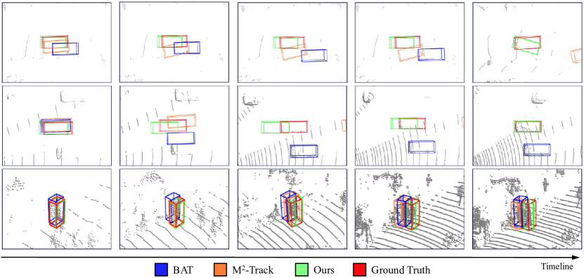
To better illustrate our method’s advantages in various scenes, we visualize some challenging scenes from the KITTI dataset, as shown in Fig. 7. In sparse and occluded scenes (the 1st and 2st rows), BAT, utilizing appearance matching, and M2-Track, relying on instance-level motion estimation, gradually lose track of the target. In contrast, our method utilizes the abundant target information from historical frames to provide prior knowledge for model tracking, which aids in recapturing the target once the point clouds become denser. In scenes with interference from similar objects (3st row), our point-level flow motion estimation captures finer local motions, thereby better distinguishing interfering objects and enhancing tracking performance.
IV-D Ablation Study
To validate the effectiveness of our proposed modules, including Historical Information Fusion(HIM), Point-level Motion Modole(PMM) and Instance Flow Head(IFH), we conduct ablation studies on the Car of the KITTI dataset.
Model Components. Firstly, we conduct an ablation study on the main components of our method to explore the effects of each module. As shown in Tab. IV, A1 represents all network models of our method. In A2, the removal of the HIM results in a performance decrease of 3.6%/3.8% in success/precision. This result demonstrates that the HIM effectively aggregates historical information, thereby improving the tracking performance of the network. In A3, when we remove the PMM, the model’s performance shows a significant decline, with success and precision decreasing by 11.2% and 10.9% respectively. This demonstrates the critical importance of multiscale point-level flow in target motion prediction, as it comprehensively captures the local motion details of the target. In A4, we replace the IFH with a traditional center head [28] and observe a decrease of 3.4%/3.3% in Success/Precision, respectively. It is evident that IFH accurately transforms dense point-level flow into instance-level motion, thereby enhancing tracking performance.
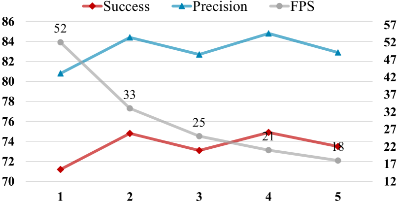
Input History Frames. To explore the impact of the number of historical frames on the model’s performance, we conducted an ablation experiment by adjusting the input historical frames. As illustrated in Fig. 8, our method showed significant enhancement as the historical frames increased from 1 to 2, improving performance by 3.6%/3.5%. However, as the historical frames increased further, performance fluctuated around 73.8%/83.5%. Earlier historical frames do not always contribute positively to the tracking of the target due to their inclusion of outdated target states. Additionally, an excessive number of historical frames can increase computational complexity and reduce the model’s speed. Hence, to balance speed and performance, we adopt the default setting of two history frames as input for our method, maintaining a performance of 33 FPS.
Comparison in Historical Frames Fusion. As shown in Tab. V, We conducted experimental comparisons on different historical frames fusion methods to validate the effectiveness of the HFM. In B1, we directly concatenate all historical frames along the feature channels. In B2, we employ a cross-attention mechanism, using as the query and as key and value. In B3, the HIF uses the learnable target feature as a bridge to achieve efficient information interaction between tracking targets across frames. The performance of the concatenation in B1 and the attention mechanism in B2 has decreased by 3.0%/2.9% and 2.7%/2.7% when compared to the HIF in B3. We believe that the operation of directly concatenating features from historical frames in B1 is overly simplistic for information aggregation, as it overlooks the alignment of target features across multiple frames. While the cross-attention in B2 achieves inter-frame information interaction, the feature interaction across the entire feature maps often introduces interference from background information. By using the learnable target feature, the HIF can more effectively focus on the feature fusion of target information within the frame, significantly reducing background information interaction and achieving superior results.
| Methods | 3D Success | 3D Precision | |
|---|---|---|---|
| B1 | Concatenation | 71.8 | 81.5 |
| B2 | Attention | 72.1 | 81.7 |
| B3 | HIF | 74.8 | 84.4 |
| Methods | 3D Success | 3D Precision | |
|---|---|---|---|
| C1 | Center Head | 71.4 | 81.1 |
| C2 | MLP | 70.0 | 80.4 |
| C3 | Instance Flow Head | 74.8 | 84.4 |
Comparison in Head Methods. In the Tab. VI, we compared the impact of different prediction heads on the model’s performance. In comparison to our proposed Instance Flow head, adopting the Center Head, MLP led to performance drops of 3.4%/3.3% and 4.8%/4.0%, respectively. The prediction heads in C1 and C2 do not effectively consider the transformation relationship from dense point-level flow motion to instance-level target motion, thereby leading to a decline in performance. In contrast, our IFH achieves accurate transformation between the two by adaptively predicting flow weight maps.
V Conclusion
In this paper, we propose a multi-frame point-level flow tracking network, FlowTrack, which achieves target tracking by capturing the local motion information of the target. Simultaneously, the proposed HIF and IFH effectively aggregate target information across temporal dimensions and convert the point-level flow of target to instance-level motion. Extensive experiments demonstrate that our method outperforms previous matching and motion paradigm methods, achieving competitive performance on the KITTI and NuScenes datasets.
References
- [1] L. Bertinetto, J. Valmadre, J. F. Henriques, A. Vedaldi, and P. H. S. Torr, “Fully-convolutional siamese networks for object tracking,” in ECCV Workshops (G. Hua and H. Jégou, eds.), pp. 850–865, 2016.
- [2] B. Li, J. Yan, W. Wu, Z. Zhu, and X. Hu, “High performance visual tracking with siamese region proposal network,” in IEEE/CVF CVPR, pp. 8971–8980, 2018.
- [3] D. Guo, J. Wang, Y. Cui, Z. Wang, and S. Chen, “Siamcar: Siamese fully convolutional classification and regression for visual tracking,” in Proceedings of the IEEE/CVF conference on computer vision and pattern recognition, pp. 6269–6277, 2020.
- [4] S. Giancola, J. Zarzar, and B. Ghanem, “Leveraging shape completion for 3d siamese tracking,” in Proceedings of the IEEE/CVF Conference on Computer Vision and Pattern Recognition, 2019.
- [5] H. Qi, C. Feng, Z. Cao, F. Zhao, and Y. Xiao, “P2b: Point-to-box network for 3d object tracking in point clouds,” in IEEE/CVF Conference on Computer Vision and Pattern Recognition, 2020.
- [6] L. Hui, L. Wang, L.-Y. Tang, K. Lan, J. Xie, and J. Yang, “3d siamese transformer network for single object tracking on point clouds,” in European Conference on Computer Vision, 2022.
- [7] C. Zheng, X. Yan, H. Zhang, B. Wang, S. Cheng, S. Cui, and Z. Li, “Beyond 3d siamese tracking: A motion-centric paradigm for 3d single object tracking in point clouds,” in Proceedings of the IEEE/CVF Conference on Computer Vision and Pattern Recognition, pp. 8111–8120, 2022.
- [8] Y. Xia, Q. Wu, W. Li, A. B. Chan, and U. Stilla, “A lightweight and detector-free 3d single object tracker on point clouds,” IEEE Transactions on Intelligent Transportation Systems, vol. 24, no. 5, pp. 5543–5554, 2023.
- [9] Z. Teed and J. Deng, “Raft: Recurrent all-pairs field transforms for optical flow,” in Computer Vision–ECCV 2020: 16th European Conference, Glasgow, UK, August 23–28, 2020, Proceedings, Part II 16, pp. 402–419, Springer, 2020.
- [10] A. Luo, F. Yang, X. Li, L. Nie, C. Lin, H. Fan, and S. Liu, “Gaflow: Incorporating gaussian attention into optical flow,” in Proceedings of the IEEE/CVF International Conference on Computer Vision, pp. 9642–9651, 2023.
- [11] Y. Yan, Y. Mao, and B. Li, “Second: Sparsely embedded convolutional detection,” in Sensors, vol. 18, 2018.
- [12] L. Hui, L. Wang, M. Cheng, J. Xie, and J. Yang, “3d siamese voxel-to-bev tracker for sparse point clouds,” in Neural Information Processing Systems, 2021.
- [13] C. R. Qi, O. Litany, K. He, and L. J. Guibas, “Deep hough voting for 3d object detection in point clouds,” in Proceedings of the IEEE/CVF International Conference on Computer Vision, 2019.
- [14] C. Zhou, Z. Luo, Y. Luo, T. Liu, L. Pan, Z. Cai, H. Zhao, and S. Lu, “Pttr: Relational 3d point cloud object tracking with transformer,” 2022 IEEE/CVF Conference on Computer Vision and Pattern Recognition, pp. 8521–8530, 2021.
- [15] A. Vaswani, N. Shazeer, N. Parmar, J. Uszkoreit, L. Jones, A. N. Gomez, L. u. Kaiser, and I. Polosukhin, “Attention is all you need,” in Advances in Neural Information Processing Systems, vol. 30, Curran Associates, Inc., 2017.
- [16] Y. Cui, Z. Li, and Z. Fang, “Sttracker: Spatio-temporal tracker for 3d single object tracking,” IEEE Robotics and Automation Letters, vol. 8, pp. 4967–4974, 2023.
- [17] M. J. Black and P. Anandan, “A framework for the robust estimation of optical flow,” in 1993 (4th) International Conference on Computer Vision, pp. 231–236, IEEE, 1993.
- [18] A. Bruhn, J. Weickert, and C. Schnörr, “Lucas/kanade meets horn/schunck: Combining local and global optic flow methods,” International journal of computer vision, vol. 61, pp. 211–231, 2005.
- [19] A. Dosovitskiy, P. Fischer, E. Ilg, P. Hausser, C. Hazirbas, V. Golkov, P. Van Der Smagt, D. Cremers, and T. Brox, “Flownet: Learning optical flow with convolutional networks,” in Proceedings of the IEEE international conference on computer vision, pp. 2758–2766, 2015.
- [20] Z. Huang, X. Shi, C. Zhang, Q. Wang, K. C. Cheung, H. Qin, J. Dai, and H. Li, “Flowformer: A transformer architecture for optical flow,” in European conference on computer vision, pp. 668–685, Springer, 2022.
- [21] T. Meinhardt, A. Kirillov, L. Leal-Taixé, and C. Feichtenhofer, “Trackformer: Multi-object tracking with transformers,” 2022 IEEE/CVF Conference on Computer Vision and Pattern Recognition, pp. 8834–8844, 2021.
- [22] Y. Zhou and O. Tuzel, “Voxelnet: End-to-end learning for point cloud based 3d object detection,” 2018 IEEE/CVF Conference on Computer Vision and Pattern Recognition, pp. 4490–4499, 2017.
- [23] J. Shan, S. Zhou, Z. Fang, and Y. Cui, “Ptt: Point-track-transformer module for 3d single object tracking in point clouds,” 2021 IEEE/RSJ International Conference on Intelligent Robots and Systems, pp. 1310–1316, 2021.
- [24] C. Zheng, X. Yan, J. Gao, W. Zhao, W. Zhang, Z. Li, and S. Cui, “Box-aware feature enhancement for single object tracking on point clouds,” 2021 IEEE/CVF International Conference on Computer Vision, pp. 13179–13188, 2021.
- [25] Y. Cui, J. Shan, Z. Gu, Z. Li, and Z. Fang, “Exploiting more information in sparse point cloud for 3d single object tracking,” IEEE Robotics and Automation Letters, vol. 7, no. 4, pp. 11926–11933, 2022.
- [26] J. Nie, Z. He, Y. Yang, M. Gao, and J. Zhang, “Glt-t: Global-local transformer voting for 3d single object tracking in point clouds,” in Proceedings of the AAAI Conference on Artificial Intelligence, vol. 37, pp. 1957–1965, 2023.
- [27] J. Gao, X. Yan, W. Zhao, Z. Lyu, Y. Liao, and C. Zheng, “Spatio-temporal contextual learning for single object tracking on point clouds,” IEEE Transactions on Neural Networks and Learning Systems, pp. 1–13, 2023.
- [28] T. Yin, X. Zhou, and P. Krahenbuhl, “Center-based 3d object detection and tracking,” in Proceedings of the IEEE/CVF conference on computer vision and pattern recognition, pp. 11784–11793, 2021.
- [29] A. Geiger, P. Lenz, and R. Urtasun, “Are we ready for autonomous driving? the kitti vision benchmark suite,” in IEEE Conference on Computer Vision and Pattern Recognition, pp. 3354–3361, 2012.
- [30] H. Caesar, V. Bankiti, A. H. Lang, S. Vora, V. E. Liong, Q. Xu, A. Krishnan, Y. Pan, G. Baldan, and O. Beijbom, “nuscenes: A multimodal dataset for autonomous driving,” in IEEE/CVF Conference on Computer Vision and Pattern Recognition, 2020.
- [31] M. Kristan, J. Matas, A. Leonardis, T. Vojíř, R. Pflugfelder, G. Fernández, G. Nebehay, F. Porikli, and L. Čehovin, “A novel performance evaluation methodology for single-target trackers,” IEEE Transactions on Pattern Analysis and Machine Intelligence, vol. 38, no. 11, pp. 2137–2155, 2016.
- [32] S. Gao, C. Zhou, C. Ma, X. Wang, and J. Yuan, “Aiatrack: Attention in attention for transformer visual tracking,” in European Conference on Computer Vision, pp. 146–164, Springer, 2022.