A Fast Multitaper Power Spectrum Estimation in Nonuniformly Sampled Time Series  

Abstract

Nonuniformly sampled signals are prevalent in real-world applications, but their power spectra estimation, usually from a finite number of samples of a single realization, presents a significant challenge. The optimal solution, which uses Bronez Generalized Prolate Spheroidal Sequence (GPSS), is computationally demanding and often impractical for large datasets. This paper describes a fast nonparametric method, the MultiTaper NonUniform Fast Fourier Transform (MTNUFFT), capable of estimating power spectra with lower computational burden. The method first derives a set of optimal tapers through cubic spline interpolation on a nominal analysis band. These tapers are subsequently shifted to other analysis bands using the NonUniform FFT (NUFFT). The estimated spectral power within the band is the average power at the outputs of the taper set. This algorithm eliminates the needs for time-consuming computation to solve the Generalized Eigenvalue Problem (GEP), thus reducing the computational load from $O(N^{4})$ to $O(N\log N+N\log(1/\epsilon))$, which is comparable with the NUFFT. The statistical properties of the estimator are assessed using Bronez GPSS theory, revealing that the bias of estimates and variance bound of the MTNUFFT estimator are identical to those of the optimal estimator. Furthermore, the degradation of bias bound may serve as a measure of the deviation from optimality. The performance of the estimator is evaluated using both simulation and real-world data, demonstrating its practical applicability. The code of the proposed fast algorithm is available on GitHub [1].

¹ Mayo Clinic Foundation, Rochester, MN 55901, USA

 Corresponding authors {Cui.Jie, Gregory.Worrell}@mayo.edu

1 Introduction

Power spectrum estimation is a fundamental tool in a wide variety of scientific disciplines [2, 3, 4, 5], including signal processing, communication, machine learning, physical science, and biomedical data analysis [6, 7]. It allows for the characterization of the second moments of a time series, elucidating periodicities, oscillatory behavior, and correlation structures in a signal process. These attributes are crucial to numerous applications.

Despite its extensive lineage [2], power spectrum estimation continues to be an active research domain. The primary challenge resides in estimating the spectrum in a way to minimize bias and ensure statistical robustness, often from a finite sample of the signal. In many instances, only a single realization or trial of the underling process is available. Spectrum estimation can be seen as an inverse problem [8, 9], and the limitation of samples necessitates an approximate solution. This constraint can lead to significant sidelobe leakage and bias in the estimates. Along with the single realization issue, a simple power estimation, such as the periodogram [10], usually suffers from large variance. In addition, in many real-world applications, the signal is often nonuniformly sampled. This includes scenarios such as network packet data transfer [11], laser Doppler anemometry [12, 13], geophysics [14], astronomy [15, 16, 17, 18], computer tomography [19], genetics [20], and biological signals [21, 22, 23, 24]. Nonuniform sampling tends to exacerbate sidelobe leakage, leading to inflated bias [25].

This paper focuses on a nonparametric solution to the power spectrum estimation problem, in contrast to the parametric ones that assumes a specific model of the time series [4]. Nonparametric methods are particularly suitable for rapid, exploratory analysis of large datasets, especially when the underlying model is unknown. In such cases, Thomson’s multitaper method proves to be a powerful tool [8]. This method employs the Discrete Prolate Spheroidal Sequences (DPSS) [26], denoted as $v_{n}^{(k)}(N,f_{w})$, where $k$, for $1\leq k\leq K$, denotes the kth DPSS sequence, $N$ the signal length, and $f_{w}$ the half bandwidth. Basically, the method initially computes the Discrete Fourier Transform (DFT) of the uniformly sampled signal, $x(n)$, $1\leq n\leq N$, weighted by the DPSS,

$$J_{k}(f)=\sum_{n=1}^{N}\left[x(n)v_{n}^{(k)}(N,f_{w})\right]e^{-j2\pi fn/f_{s}},$$ (1)

where $f_{s}$ is the sampling frequency. The power spectrum estimate is then computed as an average of the square of eigencoefficients $J_{k}(f)$, $|J_{k}(f)|^{2}$, known as the $k$th eigenspectrum,

$$\hat{P}(f)=\frac{1}{K}\sum_{k=1}^{K}\left|J_{k}(f)\right|^{2}.$$ (2)

In practice, an adaptively weighted average of the $|J_{k}(f)|^{2}$’s is available [8, 4]. Thomson’s approach achieves an optimal balance between bias and variance while maintaining a given resolution, among many other benefits [27, 28, 4, 51, 30].

Extending the multitaper scheme to nonuniformly sampled signal is desirable. However, the traditional approach is not readily applicable, as the performance of the estimator in a general sampling scheme depends on more than just the frequency resolution. Lepage (2009) [31] proposed a direct generalization of Thomson’s original approach [8], replacing the DFT with the “irregular DFT (irDFT)” and subsequently replacing the Dirichlet-type kernel with a sampling scheme-dependent, Hermitian, Toeplitz kernel. This method demonstrated superior performance compared to competitive multitaper estimates computed from the uniformly sampled data using interpolation. Springford (2020) [17] adapted the Thomson multitaper method to enhance the estimation from the Lomb-Scargel (LS) periodogram [15, 16], a technique widely employed in astronomy. Dodson-Robinson and Haley (2023) [18] examined the performance of the multitaper Lomb-Scargle (MTLS) periodogram for scenarios with missing-data and further suggested the application of an F-test to assess periodicity in nonuniformly sampled data. While these approaches have merit in various aspects, a comprehensive evaluation of their statistical performance in terms of bias, variance, and optimality has not been adequately evaluated. Additionally, the computational cost of these methods has not been explicitly addressed.

In contract, the seminal work by Bronez (1985, 1988) [32, 33] proposed an optimal estimator based on the study of the first and second moments of quadratic spectral estimator (see Section 2) for arbitrary sampling times. This method calculates the optimal weight sequence (or taper) for each analysis band, known as the Generalized Prolate Spheroidal Sequence (GPSS), by solving a Generalized Eigenvalue Problem (GEP). This work established an optimality criterion for the performance of power spectrum estimators in the general case of sampling schemes. However, since the number of analysis bands is in general proportional to $N$, and the GPSS has to be estimated for each analysis band, the computational cost is prohibitively high for large $N$.

In this study, we developed a fast algorithm for power spectrum estimation by integrating the approaches of both Thomson’s and Bronez’s multitaper estimators. Specifically, we first replaced the DPSS, $v_{n}^{(k)}(N,f_{w})$, in (1) with the GPSS, $w_{k}^{0}(t_{n})$, for $1\leq n\leq N$, from a nominal analysis band $\mathcal{A}_{0}$ (see Section 3 for details). Subsequently, the eigencoefficients $J_{k}(\mathcal{A}_{i})$, for $1\leq k\leq K$ and $0\leq i\leq I-1$, were computed using Nonuniform Fast Fourier Transform (NUFFT), and estimated power, $\hat{P}(\mathcal{A}_{i})$, was derived from a direct average across the $K$ squared eigencoefficients $|J_{k}(\mathcal{A}_{i})|^{2}$.

To further minimize the computational cost, we approximated the GPSS, $\widehat{w}_{k}^{0}(t_{n})$, by interpolating the uniformly spaced $v_{n}^{(k)}(N,f_{w})$ to the nonuniform grid $t_{n}$ with cubic spline. As a result, the overall computational complexity is compatible with that of fast NUFFT, which is approximately $O(N\log N+N\log(1/\epsilon))$, where $\epsilon$ is the precision of computations.

Importantly, we evaluated the statistical properties of the proposed method in terms of bias, variance, and suboptimality based on the theory developed in Bronez GPSS [33]. We found that the bias and variance bounds were compatible with the optimal method. We also propose that the suboptimality of the fast algorithm may be quantified using the difference between the approximate and optimal eigenvalues. Furthermore, an F-test have been implemented to test periodicity in nonuniformly sampled time series.

The reminder of the paper is organized as follows. We provide an overview of the Bronez GPSS method in Section 2, serving as the background information for the following derivations. In Section 3 we develop the fast MTNUFFT algorithm and evaluate its statistic properties in the context of Bronez GPSS theory. The performance evaluation of the estimator, which includes both simulation results and a real-world application, is presented in Section 4. The paper concludes with a discussion in Section 5 and final remarks in Section 6. The MATLAB (MathWorks, Natick, MA) code of the fast algorithm (MTNUFFT, Table 1) is publicly available on GitHub [1].

2 Bronez GPSS Optimal Approach

The Bronez GPSS (BG) is an extension of the quadratic spectral estimator, developed to analyze nonuniformly sampled processes [32, 33]. It is an optimal nonparametric method in the sense that it is unbiased in the context of white noise, and it minimizes the variance and bias bounds for a given frequency resolution.

Consider $x(t_{n})$ a weakly stationary, band-limited Gaussian process, available on a set of arbitrary sampling points $t_{n}$, $1\leq n\leq N$, where $N$ is the total number of samples. Instead of directly estimating the spectral density, $S(f)$, BG estimates the power, $P(\mathcal{A})=\int_{\mathcal{A}}S(f)\,df$, contained in an analysis band of interest $\mathcal{A}=\{f:|f-f_{c}|\leq f_{w}\}$, where $f_{c}$ is the center frequency and $f_{w}$ the half bandwidth. Note that $2f_{w}$ is the desired frequency resolution. A complete spectral analysis involves estimating $P(\mathcal{A})$ for a set of analysis bands, $\mathcal{A}$, to cover the entire signal band $\mathcal{B}=\{f:|f|\leq f_{\max}\}$, where $f_{\max}$ is presumably the maximum frequency of the signal. The estimator can be expressed as

$$\hat{P}(\mathcal{A})=\frac{1}{K}\mathbf{x}^{*}\mathbf{Q}(\mathcal{A})\mathbf{x},$$ (3)

where $\mathbf{x}=[x(t_{1}),x(t_{2}),\ldots,x(t_{n})]^{\prime}$, the prime ^′ denotes vector transposition, and the asterisk $*$ denotes complex conjugate transposition. $\mathbf{Q(\mathcal{A})}$ is an $N\times N$ positive semidefinite Hermitian weight matrix that depends on the analysis band $\mathcal{A}$. Here, $K\leq N$ is the rank of $\hat{P}(\mathcal{A})$. $\mathbf{Q(\mathcal{A})}$ can be factorized as $\mathbf{Q(\mathcal{A})}=\mathbf{\Psi}(\mathcal{A})\mathbf{\Psi}^{*}(\mathcal{A})$, where $\mathbf{\Psi}(\mathcal{A})$ is an $N\times K$ matrix. The power spectrum estimator is then given by

$$\hat{P}(\mathcal{A})=\frac{1}{K}\sum_{k=1}^{K}\left|\mathbf{w}_{k}^{*}(\mathcal{A})\mathbf{x}\right|^{2},$$ (4)

where $\mathbf{w}_{k}(\mathcal{A})$, $1\leq k\leq K$, is the columns of $\mathbf{\Psi}(\mathcal{A})$.

Assuming that the number of weight sequences, also known as tapers, $K$ is predetermined, the optimal tapers $\mathbf{w}_{k}(\mathcal{A})$ are derived base on the constraints imposed on estimator bias, variance bound, and bias bound.

2.1 Bias Constraint

The estimator, as defined in (4), is constrained to be unbiased when the true spectral density is flat, e.g., $S(f)=1$. Given the expectation of the estimate

$$E\{\hat{P}(\mathcal{A})\}=\int_{-f_{\max}}^{f_{\max}}\frac{S(f)}{K}\sum_{k=1}^{K}\left|W_{k}(f)\right|^{2}\,df,$$ (5)

where $W_{k}(f)$ is the DFT of $\mathbf{w}_{k}(\mathcal{A})$,

$$\mathbf{w}_{k}(\mathcal{A})=[w_{k}(t_{1}),w_{k}(t_{2}),\ldots,w_{k}(t_{n})],$$

$$W_{k}(f)\triangleq\sum_{n=1}^{N}w_{k}(t_{n})e^{-j2\pi ft_{n}},$$ (6)

to minimize the bias, $E\{\hat{P}(\mathcal{A})\}-P(\mathcal{A})$, the weight sequences, $\mathbf{w}_{k}(\mathcal{A})$, must satisfy

$$\int_{-f_{\max}}^{f_{\max}}\frac{1}{K}\sum_{k=1}^{K}\left|W_{k}(f)\right|^{2}\,df=\int_{f_{c}-f_{w}}^{f_{c}+f_{w}}\,df,$$ (7)

which is equivalent to

$$\frac{1}{K}\sum_{k=1}^{K}\mathbf{w}_{k}^{*}(\mathcal{A})\mathbf{R}(\mathcal{B})\mathbf{w}_{k}(\mathcal{A})=2f_{w}.$$ (8)

$\mathbf{R}(\mathcal{B})$ is the GPSS matrix on signal band $\mathcal{B}$. It is an $N\times N$ positive definite Hermitian matrix, whose elements are

$$\mathbf{R}(\mathcal{B};n,m) =\int_{-f_{\max}}^{f_{\max}}e^{j2\pi f(t_{n}-t_{m})}df$$

$$=\frac{\sin\left[2\pi f_{\max}(t_{n}-t_{m})\right]}{\pi(t_{n}-t_{m})}.$$ (9)

2.2 Variance Bound

For a Gaussian process, the variance of the estimator can be bounded above by

$$VAR\{\hat{P}(\mathcal{A})\}\leq S_{\max}^{2}\cdot V\{\mathbf{w}_{1}(\mathcal{A}),\ldots,\mathbf{w}_{K}(\mathcal{A})\},$$

where $S_{\max}=\sup_{f\in\mathcal{[}B]}S(f)$ is the maximum value of the spectral density, and $V{\{\mathbf{w}_{k}(\mathcal{A})\}}_{k=1}^{K}$ is the bound factor

$$\mathbb{V}\{\mathbf{w}_{1}(\mathcal{A}),\ldots,\mathbf{w}_{K}(\mathcal{A})\}$$

$$\quad=\frac{1}{K^{2}}\sum_{k=1}^{K}\sum_{l=1}^{K}\left|\int_{-f_{\max}}^{f_{\max}}{W_{k}(f)}^{*}{W_{l}(f)}\,df\right|^{2}$$

$$\quad=\frac{1}{K^{2}}\sum_{k=1}^{K}\sum_{l=1}^{K}\left|\mathbf{w}_{k}^{*}(\mathcal{A})\mathbf{R}(\mathcal{B})\mathbf{w}_{l}(\mathcal{A})\right|^{2}.$$ (10)

Choosing the weight sequence to minimize (10), while satisfying (8), leads to the sequence normalization requirement

$$\mathbf{w}_{k}^{*}(\mathcal{A})\mathbf{R}(\mathcal{B})\mathbf{w}_{k}(\mathcal{A})=2f_{w}\quad 1\leq k\leq K.$$ (11)

2.3 Bias Bound

By considering only the broad band errors, the errors due to frequencies outside analysis band $\mathcal{A}$, an approximate bias of estimation can be bounded above by

$$\widehat{BIAS}\{\hat{P}(\mathcal{A})\}\leq S_{\max}\cdot\mathbf{B}\{\mathbf{w}_{1},\ldots,\mathbf{w}_{k}\}$$ (12)

Given the normalization requirement (11), choosing $\mathbf{w}_{k}(\mathcal{A})$ to minimize the bound factor

$$\mathbb{B}\{\mathbf{w}_{1},\ldots,\mathbf{w}_{k}\}$$

$$\quad=\int_{-f_{\max}}^{f_{\max}}\frac{1}{K}\sum_{k=1}^{K}\left|W_{k}(f)\right|^{2}\,df-\int_{f_{c}-f_{w}}^{f_{c}+f_{w}}\frac{1}{K}\sum_{k=1}^{K}\left|W_{k}(f)\right|^{2}\,df$$

$$\quad=\frac{1}{K}\sum_{k=1}^{K}\mathbf{w}_{k}^{*}(\mathcal{A})[\mathbf{R}(\mathcal{B})-\mathbf{R}(\mathcal{(}A))]\mathbf{w}_{k}(\mathcal{A})$$ (13)

results in the GEP

$$\mathbf{R}(\mathcal{A})\mathbf{w}_{k}(\mathcal{A})=\lambda_{k}^{\mathcal{A}}\mathbf{R}(\mathcal{B})\mathbf{w}_{k}(\mathcal{A}),\quad 1\leq k\leq K,$$ (14)

where $\mathbf{R}(\mathcal{B})$ is the GPSS matrix on the signal band shown in (9) and $\mathbf{R}(\mathcal{A})$ is the GPSS matrix on the analysis band

$$\mathbf{R}(\mathcal{A};n,m) =\int_{f_{c}-f_{w}}^{f_{c}+f_{w}}e^{j2\pi f(t_{n}-t_{m})}df$$

$$=\frac{\sin\left[2\pi f_{w}(t_{n}-t_{m})\right]}{\pi(t_{n}-t_{m})}e^{j2\pi f_{c}(t_{n}-t_{m})}.$$ (15)

The GEP (14) has $N$ independent solutions $\{\lambda_{k}^{\mathcal{A}},\mathbf{w}_{k}(\mathcal{A})\}$, $1\leq k\leq N$, for the analysis band $\mathcal{A}$. The weight sequences corresponding to the $K$ largest eigenvalues are chosen to minimize the bound factors.

The computation of the GEP (14) requires $O(N^{3})$ operations for each analysis band of interest. In general, the number of bands is proportional to the number of samples, $N$, and thus makes the total computational load on the order of $O(N^{4})$. The computational demand may be impractical when $N$ is large.

3 Multitaper Nonuniform Fast Fourier Transform

In this section, we present the Multitaper Nonuniform Fast Fourier Transform (MTNUFFT) method, which is particularly effective for rapid power spectrum estimation in nonuniformly sampled time series. The derivation of this method assumes that the series follows a weakly-stationary, band-limited Gaussian process, similar to previously introduced methods [32, 33]. The number of weight sequences, or tapers, denoted as $K$, is predetermined and correlates with the properties of the tapers obtained. We will evaluate the statistical performance of the estimator based on bias measure, variance bound, and sidelobe leakage. The quantification of leakage may serve as a measure of suboptimality.

Each analysis band, $\mathcal{A}_{i}$, is defined by its center frequency $f_{c_{i}}$ and half bandwidth $f_{w}$,

$$\mathcal{A}_{i}=\left\{f:|f-f_{c_{i}}|\leq f_{w}\right\},\quad 0\leq i\leq I-1,$$ (16)

where $I$ is the total number of analysis bands. An analysis band is a subset of the signal band $\mathcal{B}=\{f:-f_{\max}\leq f\leq f_{\max}\}$, i.e., $\mathcal{A}_{i}\subset\mathcal{B},\,\forall i$. These bands are identical except for a frequency shift, and the frequency resolution $|\mathcal{A}_{i}|=2f_{w}$ is consistent across all bands. As discussed in Section 2, the primary computational cost in the Bronez GPSS method lies in the adaptive estimation of the tapers at each analysis band. To alleviate this computational burden, we propose applying the optimal tapers $\{\mathbf{w}_{k}^{0}\}_{k=1}^{K}$ at the analysis band $\mathcal{A}_{0}$ centered at $f_{c_{0}}=0$ to all other analysis bands (Fig. 1). This approach forms the estimates for each band without the need for obtaining frequency-dependent tapers.

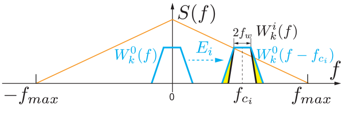
Figure 1: Frequency-Domain Transform Shift in Weighting Sequence. The figure illustrates the shift in the frequency-domain transform of the optimal weighting sequence, $W_{k}^{0}(f)$, from $f=0$ (represented by the light blue trapezium) to an analysis band centered at $f_{c_{i}}$. The bandwidth of the analysis band is $2f_{w}$. $E_{i}$ denotes the shifting operator. A dark trapezium represents the frequency-domain transform of the optimal weighting sequence, $W_{k}^{i}(f)$, centered at $f_{c_{i}}$ as per Bronez GPSS approach [32, 33]. The yellow shades indicate the sidelobe leakage difference (suboptimality) between $W_{k}^{i}(f)$ and $W_{k}^{0}(f-f_{c_{i}})$. The orange triangle in the figure represents the signal power spectrum, $S(f)$.

3.1 MTNUFFT Estimator

In this study, we designate $\mathcal{A}_{0}$ as the nominal analysis band. The corresponding optimal tapers, denoted as $\{\mathbf{w}_{k}^{0}\}_{k=1}^{K}$, are determined by solving the GEP (14) at $f_{c_{0}}$,

$$\mathbf{R}(\mathcal{A}_{0})\mathbf{w}_{k}^{0}=\lambda_{k}^{0}\mathbf{R}(\mathcal{B})\mathbf{w}_{k}^{0},\quad 1\leq k\leq K,$$ (17)

where $\{\lambda_{k}^{0},\mathbf{w}_{k}^{0}\}$ represents the kth pair of eigenvalue and eigenvector for $\mathcal{A}_{0}$. The elements of the $N\times N$ positive definite Hermitian matrix $\mathbf{R}(\mathcal{A}_{0})$ are given by

$$\mathbf{R}(\mathcal{A}_{0};n,m) =\int_{-f_{w}}^{f_{w}}e^{j2\pi f(t_{n}-t_{m})}df$$

$$=\frac{\sin\left[2\pi f_{w}(t_{n}-t_{m})\right]}{\pi(t_{n}-t_{m})}.$$ (18)

We define the shifting operator $E_{i}$ as $E_{i}=\text{diag}(\exp(j2\pi f_{c_{i}}t_{n}))$, for $1\leq n\leq N$, which leads to

$$J_{k}(\mathcal{A}_{i}) ={\mathbf{w}_{k}^{i}}^{*}\mathbf{x}={\left(E_{i}\mathbf{w}_{k}^{0}\right)}^{*}\mathbf{x}$$

$$=\sum_{n=1}^{N}\left[w_{k}^{0}(t_{n})x(t_{n})\right]e^{-j2\pi f_{c_{i}}t_{n}}.$$ (19)

The power spectrum estimator is then given by

$$\hat{P}(\mathcal{A}_{i})=\frac{1}{K}\sum_{k=1}^{K}\left|J_{k}(\mathcal{A}_{i})\right|^{2}.$$ (20)

Equation (19), known as the eigencoefficients [4], is typically implemented using nonuniform FFT (NUFFT) [34, 35]. A relevant work to the NUFFT is the Nonuniform Discrete Fourier Transform (NDFT) [36] of a time series, which is defined as samples of its $z$-transfrom evaluated at distinct points located nonuniformly on the unit circle in the $z$-plane.

3.2 Bias Measure

We began by evaluating the performance of the estimator (20) in terms of bias. This assessment was carried out under the condition that the signal is white, meaning the true spectral density is flat, as previously used in Bronez GPSS approach [33]. Specifically, we consider the case where $S(f)=1$. The expectation of the estimator can be expressed as

$$\mathbb{E}\left[\hat{P}(\mathcal{A}_{i})\right] =\int_{-f_{\max}}^{f_{\max}}S(f)\frac{1}{K}\sum_{k=1}^{K}\left|W_{k}^{i}(f)\right|^{2}df$$

$$=\int_{-f_{\max}}^{f_{\max}}\frac{1}{K}\sum_{k=1}^{K}\left|W_{k}^{0}(f)\right|^{2}df$$

$$=\frac{1}{K}\sum_{k=1}^{K}{\mathbf{w}_{k}^{0}}^{*}\mathbf{R}(\mathcal{B})\mathbf{w}_{k}^{0}=2f_{w}.$$ (21)

Here, the last equation follows from the normalization requirement (11), where $\mathbf{w}_{k}^{0}$ is optimal at $\mathcal{A}_{0}$. The bias of the estimator is then

$$\text{BIAS}\{\hat{P}(\mathcal{A}_{i})\}=\mathbb{E}\left\{\hat{P}(\mathcal{A}_{i})\right\}-\int_{f_{c_{i}}-f_{w}}^{f_{c_{i}}+f_{w}}S(f)\,df=0.$$ (22)

3.3 Variance Bound

From (23), for Gaussian process, the bound factor may be written as

$$\mathbb{V}(\widehat{\mathbf{w}}_{1}^{i},\ldots,\widehat{\mathbf{w}}_{K}^{i}) =\mathbb{V}(E_{i}\mathbf{w}_{1}^{0},\ldots,E_{i}\mathbf{w}_{K}^{0})$$

$$=\frac{1}{K^{2}}\sum_{k=1}^{K}\sum_{l=1}^{K}\left|\int_{-f_{\max}}^{f_{\max}}{W_{k}^{0}}^{*}(f-f_{c_{i}})\right.$$

$$\quad\left.\times{W_{l}^{0}}(f-f_{c_{i}})\,df\right|^{2}.$$ (23)

If the frequency center of the tapers are not near to the boundary of signal band $\mathcal{B}$, for instance, $f_{c_{i}}$ and $\pm f_{\max}$ are separated by at least $2f_{w}$, (23) may be approximated as

$$\mathbb{V}(\widehat{\mathbf{w}}_{1}^{i},\ldots,\widehat{\mathbf{w}}_{K}^{i}) \approx\frac{1}{K^{2}}\sum_{k=1}^{K}\sum_{l=1}^{K}\left|\int_{-f_{w}}^{f_{w}}{W_{k}^{0}}^{*}(f){W_{l}^{0}}(f)\,df\right|^{2}$$

$$=\frac{1}{K^{2}}\sum_{k=1}^{K}\sum_{l=1}^{K}\left|{\mathbf{w}_{k}^{0}}^{*}\mathbf{R}(\mathcal{B})\mathbf{w}_{k}^{0}\right|^{2}$$

$$=\frac{(2f_{w})^{2}}{K},$$ (24)

which is identical to the bound factor of the optimal approach.

3.4 Sidelobe Leakage and Suboptimality

As we transition the optimal eigenvectors (tapers) from the nominal analysis band $\mathcal{A}_{0}$ to $\mathcal{A}_{i}$, rather than using the optimal eigenvectors at the designated analysis band, it becomes crucial to understand the deviation from the optimal solution. As previously discussed, the bias measure and variance bound factor match the optimal ones, provided that the analysis band is not in proximity to $\pm f_{\max}$. We now consider the difference in bias bound factor between the optimal and our proposed solutions. We utilize this difference as a metric to indicate suboptimality of the fast algorithm (Fig. 1).

Using the identity $\mathbf{R}(\mathcal{A}_{0})=E_{i}^{*}\mathbf{R}(\mathcal{A}_{i})E_{i}$ (c.f., (3.42) in [32]), the bias bound factor can be expressed as

$$\mathbb{B}(\widehat{\mathbf{w}}_{1}^{i},\ldots,\widehat{\mathbf{w}}_{K}^{i}) =\int_{-f_{\max}}^{f_{\max}}\frac{1}{K}\sum_{k=1}^{K}\left|W_{k}^{0}(f-f_{c_{i}})\right|^{2}\,df$$

$$\quad-\frac{1}{K}\sum_{k=1}^{K}{\left(E_{i}\mathbf{w}_{k}^{0}\right)}^{*}\mathbf{R}(\mathcal{A}_{i}){\left(E_{i}\mathbf{w}_{k}^{0}\right)}$$

$$\approx\int_{-f_{\max}}^{f_{\max}}\frac{1}{K}\sum_{k=1}^{K}\left|W_{k}^{0}(f)\right|^{2}\,df$$

$$\quad-\frac{1}{K}\sum_{k=1}^{K}{\mathbf{w}_{k}^{0}}^{*}\mathbf{R}(\mathcal{A}_{0})\mathbf{w}_{k}^{0}$$

$$=\frac{1}{K}\sum_{k=1}^{K}{\mathbf{w}_{k}^{0}}^{*}[\mathbf{R}(\mathcal{B})-\mathbf{R}(\mathcal{A}_{0})]\mathbf{w}_{k}^{0}$$

$$=\frac{2f_{w}}{K}\sum_{k=1}^{K}(1-\lambda_{k}^{0}).$$ (25)

We once again assume that $\mathcal{A}_{i}$ is not near the boundary of $\mathcal{B}$. The absolute value of bound factor difference can now be readily seen as

$$|\Delta\mathbb{B}_{i}| \triangleq|\mathbb{B}(\widehat{\mathbf{w}}_{1}^{i},\ldots,\widehat{\mathbf{w}}_{K}^{i})-\mathbb{B}(\mathbf{w}_{1}^{i},\ldots,\mathbf{w}_{K}^{i})|$$

$$=\frac{2f_{w}}{K}|\sum_{k=1}^{K}(\lambda_{k}^{i}-\lambda_{k}^{0})|$$

$$\leq\frac{2f_{w}}{K}\sum_{k=1}^{K}|\lambda_{k}^{i}-\lambda_{k}^{0}|.$$ (26)

The difference (26) suggests that

$$\mathcal{E}=\frac{1}{K}\sum_{k=1}^{K}|\lambda_{k}^{i}-\lambda_{k}^{0}|$$ (27)

may serve as a measure of deviation from the optimal case. Clearly, $\mathcal{E}$ (27) is between 0 and 1 due to the eigenvalue condition $0\leq\lambda_{k}^{0},\lambda_{k}^{i}\leq 1$.

3.5 Thomson F-test for nonuniform signal

Statistical tests are often employed to ascertain the periodicity in signal. When a spectral peak is observed, it’s crucial to determine if its magnitude significantly exceeds what could arise by chance. The Thomson F-test [8] serves as an effective tool for detecting spectral lines in colored noise (i.e., mixed spectrum), including biological signals [37, 6].

The F-statistic for the nonuniformly sampled time series may be formally computed from the eigencoefficients (19). Assuming $2f_{c_{i}}>f_{w}$, the F-statistic can be derived as (c.f., pp. 496–500 in [4])

$$F_{s}=\frac{|\hat{C}_{i}|^{2}(K-1)\sum_{k=1}^{K}\left[W_{k}^{0}(0)\right]^{2}}{\sum_{k=1}^{K}\left|J_{k}(\mathcal{A}_{i})-\hat{C}_{i}W_{k}^{0}(0)\right|^{2}},$$ (28)

where $W_{k}^{0}(0)$ is the NUFFT of $\mathbf{w}_{k}^{0}$ at $f=0$, which is simply the summation of taper weights, $W_{k}^{0}(0)=\sum_{n=1}^{N}w_{k}^{0}(t_{n})$. $\hat{C}_{i}$ is the estimated amplitude at $f_{c_{i}}$, calculated as

$$\hat{C}_{i}=\frac{\sum_{k=1}^{K}J_{k}(\mathcal{A}_{i})W_{k}^{0}(0)}{\sum_{k=1}^{K}\left[W_{k}^{0}(0)\right]^{2}}.$$ (29)

The statistic in (28) follows an F-distribution, $F_{s}\sim F(2,2K-2)$, with 2 and $2K-2$ degrees of freedom. The critical value $F_{\alpha}$ for a given level $\alpha=1-p$ can be found from the inverse F-distribution. As a general guideline, it is recommended [8, 4] to set the p-value at the Rayleigh frequency $1/N$, where $N$ denotes the number of sample points.

3.6 Computational Cost and MTNUFFT Algorithm

The computation of $\mathbf{w}_{k}^{0}$ necessitates the resolution of the general eigenvalue problem (17), which requires $O(N^{3})$ computational complexity. This computation, unlike the Bronez GPSS method, is carried out only once at $\mathcal{A}_{0}$. The transition of $\mathbf{w}_{k}^{0}$ to other analysis band and the calculation of eigencoefficients (19) rely on the nonuniform Fast Fourier Transform (NUFFT), which demands $O(N\log N+N\log(1/\epsilon))$ arithmetic operations [38, 35], where $\epsilon$ is the precision of computation.

Given the sufficient regularity of the Slepians of $\mathbf{w}_{k}^{0}$ (DPSS), it is advantageous to interpolate the uniformly sampled DPSS to nonuniform grid to circumvent the computation of the general problem (17). We have therefore chosen to interpolate the DPSS using a cubic spline [17]. However, instead of normalizing the power of $\mathbf{w}_{k}^{0}$ to unity, we adhere to (11) for normalization. Fast algorithm for calculating uniformly spaced Slepians are available, and their computational complexity is compatible with FFT [4, 39]. Consequently, the overall computational cost of the fast algorithm approximates that of fast NUFFT.

The MTNUFFT method of spectral estimation in nonuniformly sampled time series is summarized in Table 1.

Table 1: MTNUFFT Method of Spectral Estimation

1	Define sampling points $t_{n},1\leq n\leq N$, time series samples $x(t_{n}),1\leq n\leq N$, signal band $\mathcal{B}=\{f:|f|\leq f_{\max}\}$, and half-bandwidth $f_{w}$.
2	Derive $\widehat{\mathbf{w}}_{k}^{0}=\{w_{k}^{0}(t_{1}),\ldots,w_{k}^{0}(t_{N})\}$ by interpolation:
	(a) Compute DPSS on a uniform sampling grid, denoted as $v_{n}^{(k)}(N,f_{w})$, where $k$ is the order of the sequence. The grid interval is determined by the average inter-sample-interval $\overline{\Delta}_{t}=(t_{N}-t_{1})/N$.
	(b) The taper weights $w_{k}^{0}(t_{n})$ at intermediate points corresponding to the nonuniform times $t_{n}$ are obtained by interpolation using a cubic spline.
	(c) Normalize the taper weights (eigenvector) such that
	$\displaystyle{\widehat{\mathbf{w}}_{k}^{0^{*}}\mathbf{R}(\mathcal{B})\widehat{\mathbf{w}}_{k}^{0}=2f_{w}},\,1\leq k\leq K$.	(11)
3	Calculate the eigencoefficients by NUFFT:
	$\displaystyle J_{k}(\mathcal{A}_{i})=\sum_{n=1}^{N}\left[w_{k}^{0}(t_{n})x(t_{n})\right]e^{-j2\pi f_{c_{i}}t_{n}}$,
	$1\leq k\leq K,\,0\leq i\leq I-1$.	(19)
4	Compute the MTNUFFT power spectrum estimator:
	$\displaystyle{\hat{P}(\mathcal{A}_{i})=\frac{1}{K}\sum_{k=1}^{K}\left|J_{k}(\mathcal{A}_{i})\right|^{2},\,0\leq i\leq I-1}$.	(20)

4 Performance Evaluation

We evaluated the performance of the proposed method, MTNUFFT, in three key aspects: accuracy, speed, and real-world applicability. Initially, we computed the Mean-Square Error (MSE) between the estimated and the actual power spectra of Gaussian white noise (GWN) under various sampling schemes. The results indicated that the error range of MTNUFFT was compatible with that of the optimal method, BGAdaptive. Subsequently, we contrasted the speed of MTNUFFT with three alternative methods. Our findings revealed that the speed of our algorithm is 2–3 orders of magnitude higher than that of the optimal method. Lastly, we applied our method to estimate the power spectrum of a real-world signal, specifically a nonuniformly sampled impedance measurement. We then compare the outcomes of Thomson’s F-test on the periodicity of both the original and resampled signals. This comparison allows us to evaluate the effectiveness of our method in practical applications.

Figure 2: Error Analysis of Spectrum Estimation Methods. Mean-square error comparison between the true spectrum (Gaussian white noise, GWN) and the estimated spectra using four estimation approaches, i.e., MTLS, BGFixed, BGAdaptive, and MTNUFFT, and the signals were sampled using four sampling schemes: (A) Uniformly Sampled, (B) Jittering, (C) Missing Data, and (D) Arithmetic Sampling. The frequency range was normalized to 0–0.5 Hz and half-band width ($f_{w}$) was set at 0.05 Hz. Error measures at 0–0.5 and 0.45–0.5 Hz were omitted due to unreliable estimation. Error band: $\pm 1$ SEM. Abbreviation: MTLS, multitaper Lomb-Scargle periodogram [17]; BGFixed, Bronez GPSS method with fixed TW [32]; BGAdaptive, adaptive Bronze GPSS method [32]; MTNUFFT, multitaper nonuniform fast Fourier transform (* proposed in this article).

4.1 Error Analysis

We assessed the accuracy of the proposed fast algorithm by comparing the estimated spectrum with the true spectrum of unit variance GWN ($\sigma^{2}=1$), which was conducted using four estimation methods (MTLS, BGFixed, BGAdaptive, and MTNUFFT) and four sampling schemes (Uniformly Sampled, Jittering, Missing Data, and Arithmetic Sampling) in a simulation setting. The frequency range was normalized to 0–0.5 Hz, assuming a maximum frequency ($f_{\text{max}}$) of 0.5 Hz in the simulated signals. The duration ($T$) of these signals was set at 50 seconds.

We adopted the sampling schemes implemented in [32] to sample 50 data points from the GWN. For uniform sampling grid, the samples were generated at one-second interval, denoted as $t_{n}=n,\ 1\leq n\leq 50$. To generate the jittering dataset [40, 5], the sampling time was defined as $t_{n}=n+z_{n}$, where the jittered displacement process $z_{n}$ was drawn from the GWN distribution with zero mean and a standard deviation of 0.1 second. The average sample number per second, known as the intensity of sampling process [5] ($\lambda$), was set to 1. For the missing-data sampling, we sampled the data at time points at $t_{n}=5n/6,\ 1\leq n\leq 60$ and omitted 10 points at $n=1,5,17,18,19,23,27,32,53,56$. The fourth dataset was generated using an arithmetic sampling, defined as $t_{n}=1+a(n-1)+b(n-1)(n-2)/2,\ 1\leq n\leq 50$, where $a=2/3$, $b=a/(50-2)$ [32].

For the multitaper scheme adopted in MTLS and MTNUFFT, we chose a half-bandwidth ($f_{w}$) at 0.05 Hz, which corresponds to a frequency resolution of 0.1 Hz and a time-half-bandwidth (TW) of 2.5. We adopted four tapers for the analysis.

In the Bronez GPSS methods (BGFixed, BGAdaptive), the signal band $\mathcal{B}$ was defined within the range of 0–0.5 Hz. For BGFixed, we set the analysis band $\mathcal{A}_{i}$ at $0.1$ Hz around each frequency center of interest $f_{c_{i}}$, where $0\leq i\leq I-1$. Conversely, for BGAdaptive, we adaptively determined the number of eigenvalues (i.e., number of tapers, $K$) and analysis bandwidth. Initially, at each frequency center, we set the number of tapers at 4, and half bandwidth at 0.05 Hz. We then increased the number of tapers iteratively until the maximum side lobe leakage of the tapers was less than -30 dB. Using the current number of tapers and analysis bandwidth, we estimated the power spectrum around the current frequency center. If the maximum leakage did not fall below -30 dB until the maximum number of tapers (set at 8) was reached, we increased the analysis bandwidth by 0.01 Hz and repeated the process. The iteration stopped when the maximum leakage was below -30 dB or when the analysis bandwidth reached 0.5 Hz. The final number of tapers and analysis bandwidth were then used to estimate the power spectrum at the current frequency center. This process was repeated for all frequency centers.

We repeated the process to evaluate the power spectrum of the GWN $M=1000$ times for each estimation method and each sampling scheme. Subsequently, we computed the MSE in decibels (dB) between the estimated spectrum $\hat{S}(f_{c_{i}})$ and true spectrum $S(f_{c_{i}})$ at each frequency center $f_{c_{i}}$, which was calculated as $\text{MSE}(f_{c_{i}})=\frac{1}{M}\sum_{m=1}^{M}{[10\log_{10}\hat{S}(f_{c_{i}})]}^{2}$, given that $S(f_{c_{i}})=1$.

Fig. 2 presents the error analysis results, organized into four panels that corresponds to the four sampling schemes. Each panel displays the mean and standard error of the mean (SEM) of squared error at each frequency center. For uniformly sampled signal, the error range was essentially identical across all four estimation methods. The MTNUFFT method demonstrated a compatible error range to the Bronez GPSS methods (BGFixed, BGAdaptive) when applied to jittering and missing-data sampling. However, the BGAdaptive method exhibited a better performance at isolated frequency centers. In the case of the arithmetic sampling scheme, the Bronez GPSS methods marginally yet significantly outperformed both MTLS and MTNUFFT across the entire signal band $\mathcal{B}$. Overall, the proposed fast algorithm, MTNUFFT, demonstrated competitive accuracy in spectrum estimation in three of the four sampling schemes investigated.

4.2 Speed Analysis

The time efficiency of the proposed method was assessed by comparing the number of spectra computed per second across four different sampling schemes, using the four spectrum estimation methods. The performance evaluation was conducted on a Windows 10 HP workstation equipped with an Intel Core i5–10500 CPU operating at 3.10 GHz and 64 GB memory. We estimated the time cost for 1,000 spectrum estimation and obtained the mean and standard deviation (STD). The results, as presented in Fig. 3, indicate that the speed of MTNUFFT is significantly surpasses that of MTLS and 2–3 orders of magnitude faster than the Bronez GPSS approaches for all four sampling schemes investigated.

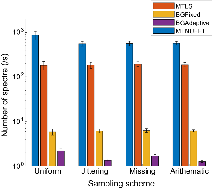
Figure 3: Speed Analysis of Spectrum Estimation Methods. This figure presents the number of spectra calculated per second for four sampling schemes using four spectrum estimation methods. The abbreviations used are consistent with those in Fig. 2. Error bar: $\pm 1$ STD

4.3 Application to Impedance Signal

To further illustrate the MTNUFFT method, we applied it to the spectral analysis of a bio-impedance signal recorded intracranially from human brain using a chronically implanted sensing and stimulation device. The specifics of the brain impedance acquisition and analysis have been detailed in our prior work [23, 24]. The impedance signal was measured using the investigational Medtronic Summit RC+S™ device with the electrodes targeting the limbic system of a patient with epilepsy. Given that the same electrodes were also utilized for delivering electric stimulation as part of neuromodulation therapy, the impedance measurements were nonuniformly sampled at an approximate rate of one sample every 15 minutes, equivalent to about 96 samples/day. Fig. 4A shows a data segment of between 150 and 160 days post device implantation (number of sample, $N=688$), which was used in the analysis. The red dots represent the original impedance samples, while the blue curve signifies the resampled signal at a uniform rate of one sample per hour ($N=240$, calculated with Matlab function resample using linear interpolation). In Panel B, the blue curve illustrates the power spectrum of the sampling instances of the original impedance signal. The decaying envelope of the sharp lines at the fundamental frequency of 96 cycles/day and its harmonics are indicative of irregular sampling [40, 41, 42]. We fitted the spectrum with a jittering model [5], assuming a normal distribution of the jittering displacement $z_{n}$ with zero mean and STD $\sigma$. The red curve in Fig. 4B represents the fitted model with mean rate $\lambda=96$ samples/day and STD $\sigma=20$ seconds, and the green dashed line indicates the mean rate at high-frequency limit. This model offers a good understanding of sampling properties of the impedance measurement sequence.

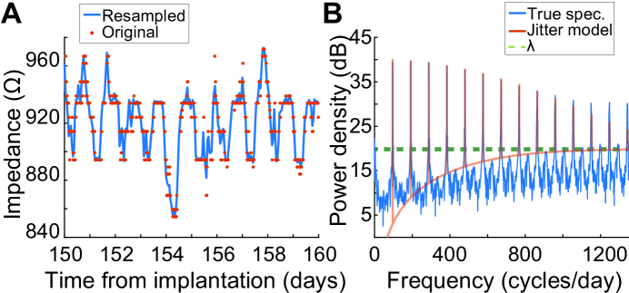
Figure 4: Impedance Signal Sampling and Jitter Model Fitting. (A) An example of impedance signal nonuniformly sampled at approximately four samples per hour using a Medtronic Summit RC+S™ neuromodulation device. Red dots represent original samples obtained 150–160 days post-implantation. The blue curve shows the resampled signal at a uniform rate of one sample per hour. (B) Power spectrum of the sampling points from (A) and its fitted model. The blue curve represents the sampling process spectrum (calculated with Chronux function mtspectrumpt, $TW=3.5$ and $K=6$), while the red curve depicts the fitted model, a uniformly sampled point process with jitter (see text for more details). The green dashed line marks the average sampling rate ($\lambda=96$ /day or $10\log_{10}(96)=19.82$ dB). Abbreviation: PSD, power spectrum density.

Subsequently, we computed the power spectra of the original signal and the resampled signal using MTNUFFT and (Chronux) mtspectrumc, respectively, under the assumption of a maximum frequency of 12 cycles/day. Identical to the calculation of point process power spectrum, the TW was set at 3.6, yielding a frequency resolution of 0.35 cycles/day, and $K$ at 6. As displayed in Fig. 5A, the spectral power of the nonuniformly sampled signal (represented by the red curve) is noticeably elevated above approximately 2 cycles/day in comparison to the spectral power of the resampled signal (blue curve). This observation aligns with previous studies [17, 31] (see Section 1: Introduction). While the spectral powers are nearly identical around the circadian cycle (1 cycle/day, indicated by arrow a) and multiday cycles ($<$ 1 cycle/day), distinct energy peaks are presented in the frequency ranges of 2–4 Hz (arrow b) and 4–6 Hz (arrow c), which are absent in the power spectrum of the resampled data. However, the elevated power at high-frequency range of 10–12 Hz (arrow d) could potentially be attributed to leakage (refer to Section 5:Discussion).

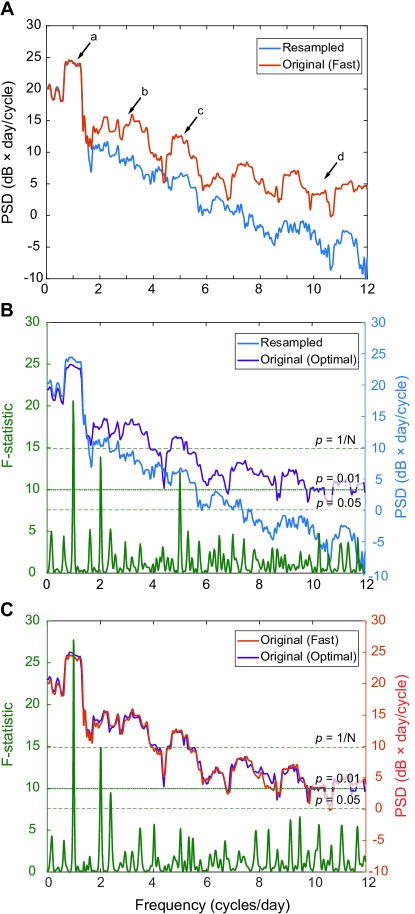
Figure 5: Spectrum and F-test Comparison. (A) Spectrum comparison. The red curve (Original (Fast)) represents the estimated power spectrum of the nonuniformly sampled impedance data (referenced as red dots in Fig. 4A) using MTNUFFT . The blue curve (Resampled) depicts the power spectrum of the resampled signal (blue curve in Fig. 4A), estimated with the Chronux [43] function mtspectrumc. The arrows point to approximate frequency bands of circadian cycles (a, 1 cycle/day), 2–4 (b), 4–6 (c), and 10–12 cycles/day (d). (B) Power spectrum of the resampled signal (blue, same as in Panel A), power spectrum of the original signal estimated with the optimal method BGFixed (purple, original (Optimal)), and Thomson periodicity F-test [8] (green) of the resampled signal. (C) Power spectrum estimated with the fast method (red, same as in Panel A, original (Fast)), power spectrum estimated with the optimal method (purple, same as in Panel B, Original (Optimal)), and F-test (green) of the original, nonuniformly sampled signal. In Panels B and C, three horizontal dashed lines represent three levels of p-values, i.e., from bottom to top, 0.05, 0.01 and $1/N$, respectively, where $N$ is the number of samples. For the resampled signal (Panel B), $N=240$, resulting in $p=0.0042$. For the original signal (Panel C), $N=688$, yielding $p=0.0015$.

Moreover, we investigated the periodicity of impedance data using the Thomson F-tests [8, 4]. Specifically, we analyzed both the original (Fig. 5B) and resampled data (Fig. 5C), where the optimal estimation of the spectrum using BGFixed is superimposed for comparison. To assess significance, we calculated critical values of the F-statistic corresponding to three significant levels: p-values at 0.05, 0.01 and the Rayleigh level ($1/N$, where $N$ is the number of samples). These critical values were derived from the F-distribution with 2 and $2K-2=10$ degrees of freedom. It is worth noting that the Rayleigh level ($p=1/N$), as recommended in Thomson et al. [8], bears similarity to the Bonferroni correction for multiple comparison [44, BRE2007]. The analysis reveals some intriguing findings. The F-statistic for the resampled signal (Panel B) indicates a strong periodicity in the circadian cycle (above the Rayleigh level) and suggests two possible cycles around 2 and 5 cycles/day (above $p=0.01$ level). In contrast, the F-statistic for the original signal confirms the robust periodicity of the circadian cycle and its harmonic at 2 cycles/day (above the Rayleigh level). Notably, it also depicts the absence of the periodicity around 5 cycles/day, raising the possibility that this suggested periodicity in the resampled signal may result from linear interpolation.

These analyses of the ultradian cycles (occurring more frequently than once per day) within impedance signals hold significant biological interest. Long-standing hypotheses propose that an ultradian basic rest-activity cycle (BARC) plays a crucial role in sleep cycles, wakefulness patterns, and the central nervous system functioning [46].

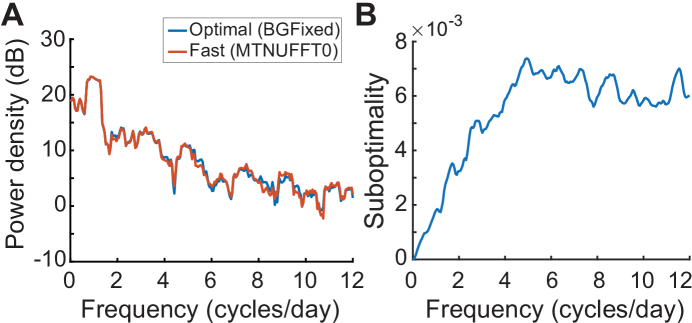
Figure 6: Spectrum comparison and suboptimality. (A) The optimal spectrum estimated with BGFixed method (blue) is compared with the spectrum estimated with the fast algorithm (red, MTNUFFT0), where the eigenvectors were $\mathbf{w}_{k}^{0},\quad 1\leq k\leq K$ (17), optimal at $\mathcal{A}_{0}$. (B) Suboptimality (27) of the spectral estimation MTNUFFT0 shown in Panel A.

Finally, we evaluated the suboptimality of the power spectrum estimation of the impedance signal by calculating $\mathcal{E}$ (27). Given that the approximate eigenvectors $\widehat{\mathbf{w}}_{k}^{0}$ lack corresponding eigenvalues, we utilized the true eigenvectors $\mathbf{w}_{k}^{0}$ at $\mathcal{A}_{0}$ for the fast algorithm MTNUFFT (see Table 1), denoted as MTNUFFT0. The power spectra, estimated by both the optimal method (BGFixed) and the fast algorithm (MTNUFFT0), are depicted in Fig. 6A. It’s important to note the identity of the spectra at $f=0$, which is confirmed by the suboptimality measure $\mathcal{E}=0$ at $f=0$, as shown in Fig. 6B. As previously discussed, suboptimality $\mathcal{E}$ is between 0 and 1, where zero signifies optimality. The larger this measure, the greater the deviation of the estimation is from the optimal scenario. The suboptimality increases as the center of the analysis band shifts away from $f=0$, but appears to plateau after about $f=5$ cycles/day. Overall, the suboptimality is less than $8\times 10^{-3}$, suggesting that the proposed method effectively estimated the power spectrum of the impedance signal.

5 Discussion

We have developed MTNUFFT, a method for the rapid estimation of the power spectrum of nonuniformly sampled time series. This method alleviates the computational burden of the Bronez GPSS in two significant ways: (a) It estimates an approximation of the optimal tapers, $\widehat{\mathbf{w}}_{k}^{0}$, at the nominal analysis band, $\mathcal{A}_{0}$, by interpolating the DPSS, $v_{n}^{(k)}(N,f_{w})$, to the nonuniform times. This eliminates the need to solve the time-consuming GEP (17). (b) It shifts $W_{k}^{0}(f)$ and calculates the eigencoefficients (19) using the NUFFT for each analysis band $\mathcal{A}_{i}$, for $0\leq i\leq I-1$. As a result, the overall computational cost aligns with the fast NUFFT, $O(N\log N+N\log(1/\epsilon))$, which is significantly lower than the cost of the optimal method, $O(N^{4})$. Simulations (Fig. 3) show that the computing speed of MTNUFFT is significantly higher than MTLS, and 2–3 orders of magnitude faster than the Bronez GPSS methods (both BGFixed and BGAdaptive).

Bronez [32, 33] also proposed a computationally efficient approximation, the Constrained-Basis Weighting Sequences approach. The basic idea is to reduce the size of the matrix in the GEP (14) from $N$ to $M$, ideally $M\ll N$. This is achieved by selecting $M$ “basis vectors” and approximating the weight sequence as $\widehat{\mathbf{w}}_{k}(\mathcal{A})=F\cdot\mathbf{c}_{k}(\mathcal{A})$, where $F$ is an $N\times M$ matrix with columns as the predefined basic vectors, and $\mathbf{c}_{k}(\mathcal{A})$ are $M\times 1$ vectors determined by solving another GEP for analysis band $\mathcal{A}$. However, the matrix size of this problem is only $M$. The vector $\mathbf{c}_{k}(\mathcal{A})$ still needs to be calculated for each analysis band. The overall computing load is in the order of $O(M^{2}N^{2})$, which can be significantly lower than $O(N^{4})$, but still notably higher than that of MTNUFFT. The choice of the basis vectors is critical to the method’s performance and requires careful consideration.

Conversely, our method, MTNUFFT, shifts the $K$ weight sequences calculated at the nominal analysis band to other analysis bands using NUFFT, which removes the computation of the GEP for each analysis band. This approach can be seen as a type of filter-based method where the power in a band is estimated as the average of the powers at the output of a filter bank consisting of $K$ filters. An interesting variation of the filter-bank approach is the Multiple Window Minimum Variance (MWMV) method [47], which minimizes the variance without applying Thomson’s adaptive weighting procedure [8]. Similar to our work, MWMV maintains the number of windows to minimize the loss in variance, while significantly reduces sidelobe leakage through linear constraints, resulting in a less biased estimate of the power. The performance of MWMV is suggested to be comparable with Thomson’s [8] and Bronez’s [32] methods. However, it involves the time-consuming computation of the covariance matrix and the computational complexity is presumably high.

Since MTNUFFT is not an optimal solution, it is crucial to evaluate the deviation from the optimal solution of its estimates. Our theoretical work (Section 3) shows that the bias of estimation and variance bound are compatible with the optimal Bronez GPSS. But the bias bound is generally degraded [48]. The suboptimality of MTNUFFT for each analysis band $\mathcal{A}_{i}$ may be quantified by the difference between $\lambda_{k}^{0}$ and $\lambda_{k}^{i}$ (27), which decreases at the expense of increasing analysis band (decrease of frequency resolution). The simulation results (Fig. 2) show that for the four sampling schemes under investigation, the error range is compatible with the optimal method for uniformly sampling, jittering and missing-data sampling. Only the error range for arithmetic sampling is consistently higher than the optimal methods. These results indicate the effectiveness of the proposed method for most practical scenarios.

It is worth noting that the variance and bias bounds may not be accurately estimated when the analysis bands are near the boundary of signal band, $f_{\max}$. In deed, a previous study [49] showed that the variance of spectrum estimates could be poorly estimated if the frequency was close to frequency limits.

The process of resampling nonuniformly sampled values to a uniform grid, for example, using linear interpolation, is often employed for spectral analysis due to the powerful tools available for estimators under uniform sampling. However, evidence suggests that this procedure could induce considerable artifacts in the power spectrum [31]. One noticeable effect of linear interpolation is a tendency for the estimated spectrum at high frequency to be lower, and at low frequency to be higher [17]. This distortion can be substantial [50]. Our analysis of the brain tissue impedance data also indicates a suppression of spectral power at higher frequencies due to interpolation. As shown in Fig. 5A, the spectrum estimated from original samples using MTNUFFT (red curve) and the spectrum estimated from the resampled signal (blue curve) are nearly identical at lower frequency ranges ($<1.5$ cycles/day), but notably different at higher frequency ranges (1.5–12 cycles/day). This observation is consistent with the previous findings and underscores the need to develop spectral estimators that directly utilize nonuniformly sampled data.

The MTNUFFT algorithm may be considered as a general framework for quickly estimating the spectrum of nonuniformly sampled signals using various types of tapers. Besides DPSS sequences, other tapers, such as minimum bias tapers and sinusoidal tapers [RIE1995, 52], have been previously suggested for different problems. Generally, these methods have not been extended to the case of nonuniformly sampled signals. By replacing the weight sequence $\mathbf{w}_{k}^{0}$ in (19) with the desired tapers, which are properly evaluated on the nonuniform sampling grid, and then applying the NUFFT and averaging (20), the MTNUFFT algorithm may be extended to these tapers for spectrum estimation in nonuniformly sampled time series. Future work will focus on extending MTNUFFT to different tapers in various data analysis scenarios and evaluating the statistical properties of the estimation.

6 Summary

This paper introduces MTNUFFT, a fast spectrum estimation method developed for nonuniformly sampled time series. The estimator comprises a set of nonuniformly sampled tapers, optimized for a nominal analysis band. The estimated power within the band is determined by averaging the power correlated to these tapers. The Nonuniform Fast Fourier Transform (NUFFT) is utilized to swiftly shift the tapers to other analysis bands of interest, thereby removing the need for the time-consuming computation involved in solving the Generalized Eigenvalue Problem (GEP) for each analysis band, a requirement for the optimal estimator, Bronez GPSS. Consequently, the overall computational cost is significantly reduced.

The statistical properties of the estimator are assessed using the Bronez GPSS theory. The results reveal that the bias of the estimates and variance bound of MTNUFFT are comparable to those of the optimal estimator. However, the limitation of MTNUFFT lies in the degradation of the bias bounds. The difference in bias bounds between MTNUFFT and the optimal estimator may serve as a measure of suboptimality. Simulation results indicate that MTNUFFT operates 2–3 orders faster than the optimal method. Moreover, the error range of MTNUFFT aligns with that of the optimal estimator in three out of four sampling schemes under investigation, suggesting effectiveness in practical applications. MTNUFFT is suitable for rapid spectrum estimation in large nonuniformly sampled datasets for exploratory analysis.

Funding

This work is supported by National Institutes of Health (NIH) grants UH3-NS095495, R01-NS092882 and R01-NS112144 (to G.W.). J.C. was also partially supported by the Epilepsy Foundation of America’s My Seizure Gauge grant (to B.H.B), the National Institutes of Health grant UG3 NS123066 (to B.H.B.), and the Mayo Clinic RFA CCaTS-CBD Pilot Awards for Team Science UL1TR000135 (to J.C.).

References

- [1] J. Cui, Code of a fast multitaper spectral estimation of nonuniformly sampled data. https://github.com/jiecui/mtnufft, 2024.
- [2] E. A. Robinson, “A historical perspective of spectrum estimation,” Proceedings of the IEEE, vol. 70, no. 9, pp. 885–907, 1982, ISSN: 0018-9219. DOI: 10.1109/PROC.1982.12423.
- [3] S. M. Kay, Modern Spectral Estimation: Theory and Application (Prentice-Hall signal processing series). Englewood Cliffs, N.J.: Prentice Hall, 1988, xv, 543 p. ISBN: 013598582X.
- [4] D. B. Percival and A. T. Walden, Spectral Analysis for Physical Applications: Multitaper and Conventional Univariate Techniques. Cambridge ; New York, NY, USA: Cambridge University Press, 1993, xxvii, 583 p. ISBN: 0521435412 (pbk.)
- [5] P. Brémaud, Fourier Analysis and Stochastic Processes. Springer International Publishing, 2014, 1 online resource (XIII, 385 pages 2 illustrations), ISBN: 9783319095905 0172-5939. DOI: 10.1007/978-3-319-09590-5.
- [6] P. P. Mitra and H. Bokil, Observed Brain Dynamics. New York: Oxford University Press, 2008, xxii, 381 p. ISBN: 9780195178081 (alk. paper).
- [7] S. V. Vaseghi, “Power spectrum analysis,” in Advanced Digital Signal Processing and Noise Reduction, 4th, Chichester; New York: JohnWiley, 2009, ch. Chapter 10, pp. 271–294, ISBN: 978-0-470-75406-1.
- [8] D. J. Thomson, “Spectrum estimation and harmonic-analysis,” Proceedings of the IEEE, vol. 70, no. 9, pp. 1055–1096, 1982, ISSN: 0018-9219.
- [9] D. J. Thomson, “Multitaper analysis of nonstationary and nonlinear time series data,” in Nonlinear and Nonstationary Signal Processing, W. J. Fitzgerald, Ed., Cambridge, UK: Cambridge University Press, 2000.
- [10] D. B. Percival, “Spectral analysis of univariate and bivariate time series,” in Statistical Methods for Physical Science, ser. Methods of Experimental Physics, J. Stanford and S. Vardeman, Eds., New York: Academic Press, 1994, pp. 313–348.
- [11] F. Eng, “Non-uniform sampling in statistical signal processing,” Dissertation, Linköping University, Linköping, Sweden, 2007.
- [12] C. Tropea, “Laser doppler anemometry: Recent developments and future challenges,” Measurement Science and Technology, vol. 6, no. 6, p. 605, 1995, ISSN: 0957-0233. DOI: 10.1088/0957-0233/6/6/001.
- [13] T. Yardibi, J. Li, P. Stoica, M. Xue, and A. B. Baggeroer, “Source localization and sensing: A nonparametric iterative adaptive approach based on weighted least squares,” IEEE Transactions on Aerospace and Electronic Systems, vol. 46, no. 1, pp. 425–443, 2010, ISSN: 1557-9603. DOI: 10.1109/TAES.2010.5417172.
- [14] M. Rauth and T. Strohmer, “A frequency domain approach to the reconvery of geophysical potenials,” in Proc. Conf. SampTA’97, Aveiro/Portugal, 1997, pp. 109–114.
- [15] N. R. Lomb, “Least-squares frequency analysis of unequally spaced data,” Astrophysics and Space Science, vol. 39, no. 2, pp. 447–462, 1976, ISSN: 1572-946X. DOI: 10.1007/BF00648343.
- [16] J. D. Scargle, “Studies in astronomical time series analysis. II. Statistical aspects of spectral analysis of unevenly spaced data,” The Astrophysical Journal, vol. 263, pp. 835i–853, 1982, ISSN: 0004-637X. DOI: 10.1086/160554.
- [17] A. Springford, G. M. Eadie, and D. J. Thomson, “Improving the Lomb-Scargle periodogram with the Thomson multitaper,” The Astronomical Journal, vol. 159, no. 5, p. 205, 2020, ISSN: 1538-3881. DOI: 10.3847/1538-3881/ab7fa1.
- [18] S. Dodson-Robinson and C. Haley, “Optimal frequency-domain analysis for spacecraft time series: Introducing the missing-data multitaper power spectrum estimator,” The Astronomical Journal, vol. 167, no. 1, p. 22, 2023, ISSN: 1538-3881. DOI: 10.3847/1538-3881/ad0c58.
- [19] H. Stark, “Polar, spiral, and generalized sampling and interpolation,” in Advanced Topics in Shannon Sampling and Interpolation Theory, ser. Springer Texts in Electrical Engineering, R. J. Marks, Ed., New York, NY: Springer US, 1993, ch. Chapter 6, pp. 185–218, ISBN: 978-1-4613-9757-1.
- [20] A.W.-C. Liew, J. Xian, S.Wu, D. Smith, and H. Yan, “Spectral estimation in unevenly sampled space of periodically expressed microarray time series data,” BMC Bioinformatics, vol. 8, no. 1, p. 137, 2007, ISSN: 1471-2105. DOI: 10.1186/1471-2105-8-137.
- [21] T. Sauer, “Reconstruction of dynamical systems from interspike intervals,” Physical Review Letters, vol. 72, no. 24, pp. 3811–3814, 1994. DOI: 10.1103/PhysRevLett.72.3811.
- [22] P. Laguna, G. B. Moody, and R. G. Mark, “Power spectral density of unevenly sampled heart rate data,” in Proceedings of 17th International Conference of the Engineering in Medicine and Biology Society, vol. 1, 1995, 157–158 vol.1. DOI: 10.1109/IEMBS.1995.575048.
- [23] F. Mivalt, V. Kremen, V. Sladky, et al., “Impedance rhythms in human limbic system,” Journal of Neuroscience, vol. 43, no. 39, pp. 6653–6666, 2023, ISSN: 0270-6474, 1529-2401. DOI: 10.1523/JNEUROSCI.0241-23.2023.
- [24] J. Cui, F. Mivalt, V. Sladky, et al., ”Acute to long-term characteristics of impedance recordings during neurostimulation in humans”, Journal of Neural Engineering, vol. 21, no. 2, p. 026022, 2024. ISSN: 1741 - 2552. DOI: 10.1088/1741-2552/ad3416.
- [25] P. Babu and P. Stoica, “Spectral analysis of nonuniformly sampled data — a review,” Digital Signal Processing, vol. 20, no. 2, pp. 359–378, 2010, ISSN: 1051-2004. DOI: 10.1016/j.dsp.2009.06.019.
- [26] D. Slepian, “Prolate spheroidal wave functions, Fourier analysis, and uncertainty—V: The discrete case,” Bell System Technical Journal, vol. 57, no. 5, pp. 1371i–1430, 1978, ISSN: 0005-8580. DOI: 10.1002/j.1538-7305.1978.tb02104.x.
- [27] L. Tauxe and G.Wu, “Normalized remanence in sediments of the western equatorial pacific: Relative paleointensity of the geomagnetic field?” Journal of Geophysical Research: Solid Earth, vol. 95, no. B8, pp. 12 337–12 350, 1990, ISSN: 2156-2202. DOI: 10.1029/JB095iB08p12337.
- [28] T. P. Bronez, “On the performance advantage of multitaper spectral analysis,” IEEE Transactions on Signal Processing, vol. 40, no. 12, pp. 2941–2946, 1992, ISSN: 1941-0476. DOI: 10.1109/78.175738.
- [29] K. S. Riedel, A. Sidorenko, and D. J. Thomson, “Spectral estimation of plasma fluctuations. I. Comparison of methods,” Physics of Plasmas, vol. 1, no. 3, pp. 485–500, 1994, ISSN: 1070-664X. DOI: 10.1063/1.870794.
- [30] B. Babadi and E. N. Brown, “A review of multitaper spectral analysis,” IEEE Transactions on Biomedical Engineering, vol. 61, no. 5, pp. 1555–1564, 2014, ISSN: 1558-2531. DOI: 10.1109/TBME.2014.2311996.
- [31] K. Lepage, “Some advances in the multitaper method of spectrum estimation,” Dissertation, Queen’s University, Kingston, ON, Canada, 2009.
- [32] T. P. Bronez, “Nonparametric spectral estimation of irregularly-sampled multidimensional processes,” Dissertation, Arizona State University, 1985.
- [33] T. P. Bronez, “Spectral estimation of irregularly sampled multidimensional processes by generalized prolate spheroidal sequences,” IEEE Transactions on Acoustics, Speech, and Signal Processing, vol. 36, no. 12, pp. 1862–1873, 1988, ISSN: 0096-3518. DOI: 10.1109/29.9031.
- [34] S. F. Potter, N. A. Gumerov, and R. Duraiswami, “Fast interpolation of bandlimited functions,” in 2017 IEEE International Conference on Acoustics, Speech and Signal Processing (ICASSP), 2017, pp. 4516–4520. DOI: 10.1109/ICASSP.2017.7953011.
- [35] A. Dutt, M. Gu, and V. Rokhlin, “Fast algorithms for polynomial interpolation, integration, and differentiation,” SIAM Journal on Numerical Analysis, vol. 33, no. 5, pp. 1689–1711, 1996, ISSN: 0036- 1429. DOI: 10.1137/0733082.
- [36] S. Bagchi and S. K. Mitra, “The nonuniform discrete Fourier transform and its applications in filter design. I. 1-D,” IEEE Transactions on Circuits and Systems II: Analog and Digital Signal Processing, vol. 43, no. 6, pp. 422–433, 1996, ISSN: 1558-125X. DOI: 10.1109/82.502315.
- [37] P. P. Mitra and B. Pesaran, “Analysis of dynamic brain imaging data,” Biophysical Journal, vol. 76, no. 2, pp. 691–708, 1999, ISSN: 0006-3495.
- [38] A. Dutt and V. Rokhlin, “Fast Fourier transforms for nonequispaced data,” SIAM Journal on Scientific Computing, vol. 14, no. 6, pp. 1368–1393, 1993, ISSN: 1064-8275. DOI: 10.1137/0914081.
- [39] S. Karnik, Z. Zhu, M. B. Wakin, J. Romberg, and M. A. Davenport, “The fast Slepian transform,” Applied and Computational Harmonic Analysis, vol. 46, no. 3, pp. 624–652, 2019, ISSN: 1063-5203. DOI: 10.1016/j.acha.2017.07.005.
- [40] M. S. Bartlett, “The spectral analysis of point processes,” Journal of the Royal Statistical Society: Series B (Methodological), vol. 25, no. 2, pp. 264–281, 1963, ISSN: 2517-6161. DOI: 10.1111/j.2517-6161.1963.tb00508.x.
- [41] M. R. Jarvis and P. P. Mitra, “Sampling properties of the spectrum and coherency of sequences of action potentials,” Neural Computation, vol. 13, no. 4, pp. 717–749, 2001, 414QX Times Cited:33 Cited References Count:25, ISSN: 0899-7667.
- [42] A. Balakrishnan, “On the problem of time jitter in sampling,” IRE Transactions on Information Theory, vol. 8, no. 3, pp. 226–236, 1962, ISSN: 2168-2712. DOI: 10.1109/TIT.1962.1057717.
- [43] H. Bokil, P. Andrews, J. E. Kulkarni, S. Mehta, and P. P. Mitra, “Chronux: A platform for analyzing neural signals,” Journal of Neuroscience Methods, vol. 192, no. 1, pp. 146–151, 2010, ISSN: 0165-0270. DOI: 10.1016/j.jneumeth.2010.06.020.
- [44] R. Christensen, “Multiple comparison techniques,” in Plane Answers to Complex Questions: The Theory of Linear Models, 4th, New York: Springer, 2011, ch. Chapter 5, pp. 105–120, ISBN: 9781441998156.
- [45] K. J. Friston, “Random field theory,” in Statistical parametric mapping: the analysis of functional brain images, M. Brett, W. Penny, and S. Kiebel, Eds., 1st, Amsterdam; Boston: Elsevier/Academic Press, 2007, ch. Chapter 18, pp. 223–231, ISBN: 9780123725608 0123725607.
- [46] N. Kleitman, “Basic rest-activity cycle—22 years later,” Sleep, vol. 5, no. 4, pp. 311–317, 1982, ISSN: 0161-8105. DOI: 10.1093/sleep/5.4.311.
- [47] T. C. Liu and B. van Veen, “Multiple window based minimum variance spectrum estimation for multidimensional random fields,” IEEE Transactions on Signal Processing, vol. 40, no. 3, pp. 578–589, 1992, ISSN: 1941-0476. DOI: 10.1109/78.120801.
- [48] R. Bellman, Introduction to Matrix Analysis (Classics in applied mathematics), 2nd. Philadelphia: Society for Industrial and Applied Mathematics, 1997, xxviii, 403 p. ISBN: 0898713994.
- [49] A. T. Walden, E. McCoy, and D. B. Percival, “The variance of multitaper spectrum estimates for real Gaussian processes,” IEEE Transactions on Signal Processing, vol. 42, no. 2, pp. 479–482, 1994, ISSN: 1941-0476. DOI: 10.1109/78.275635.
- [50] M. E. Mann and J. M. Lees, “Robust estimation of background noise and signal detection in climatic time series,” Climatic Change, vol. 33, no. 3, pp. 409–445, 1996, ISSN: 1573-1480. DOI: 10.1007/BF00142586.
- [51] K. S. Riedel and A. Sidorenko, “Minimum bias multiple taper spectral estimation,” IEEE Transactions on Signal Processing, vol. 43, no. 1, pp. 188–195, 1995, ISSN: 1941-0476. DOI: 10.1109/78.365298.
- [52] D. B. Percival and A. T. Walden, “Combining direct spectral estimators,” in Spectral Analysis for Univariate Time Series, ser. Cambridge series on statistical and probabilistic mathematics, Cambridge: Cambridge University Press, 2020, ch. Chapter 8, pp. 351–444, ISBN: 1-108-77617-5 1-139-23572-9.