Radiation MHD Simulations of Soft X-ray Emitting Regions in Changing Look AGN
Abstract
Strong soft X-ray emission called soft X-ray excess is often observed in luminous active galactic nuclei (AGN). It has been suggested that the soft X-rays are emitted from a warm () region that is optically thick for the Thomson scattering (warm Comptonization region). Motivated by the recent observations that soft X-ray excess appears in changing look AGN (CLAGN) during the state transition from a dim state without broad emission lines to a bright state with broad emission lines, we performed global three-dimensional radiation magnetohydrodynamic simulations assuming that the mass accretion rate increases and becomes around % of the Eddington accretion rate. The simulation successfully reproduces a warm, Thomson-thick region outside the hot radiatively inefficient accretion flow near the black hole. The warm region is formed by efficient radiative cooling due to inverse Compton scattering. The calculated luminosity is consistent with the luminosity of CLAGN. We also found that the warm Comptonization region is well described by the steady model of magnetized disks supported by azimuthal magnetic fields. When the anti-parallel azimuthal magnetic fields supporting the radiatively cooled region reconnect around the equatorial plane of the disk, the temperature of the region becomes higher by releasing the magnetic energy transported to the region.
1 Introduction
Luminous active galactic nuclei (AGN), such as Seyfert galaxies and quasars, exhibit soft X-ray emission. The origin of the soft X-ray emission in AGN is puzzling since the temperature of the standard accretion disk around a supermassive black hole is around (Shakura & Sunyaev, 1973). Two types of models have been proposed to explain the soft X-ray emission. One is the ionized reflection model (e.g., Gierliński & Done, 2004; García et al., 2019). In this model, the soft X-ray emission is emitted by an optically thick disk that is irradiated by the hard X-ray emission from the vicinity of the central black hole. Another model is the emission from the Thomson thick warm corona with temperature by inverse Compton scattering (e.g,. Magdziarz et al., 1998; Done et al., 2012). Kubota & Done (2018) showed that the intensity of the soft X-ray emission increases with increasing the mass accretion rate. However, the geometry of the warm Comptonization region is still unknown, and it is not clear whether it is a region separated from the cool optically thick disk or associated with the cool disk.
Recent monitoring observations have shown that some Seyfert galaxies exhibit spectral state transitions (e.g., Shappee et al., 2014; Ricci et al., 2020). They show transitions between a state without broad emission lines in the optical range (type 2 AGN) and a state with broad emission lines (type 1 AGN) (e.g., Shapovalova et al., 2019; Oknyansky et al., 2020; Popović et al., 2023). During the state transitions, the UV to X-ray spectrum also shows transitions (e.g., Ricci et al., 2021). AGN that shows state transitions between type 1 and type 2 are called changing look AGN (CLAGN; see Ricci & Trakhtenbrot, 2023). Noda & Done (2018) and Tripathi & Dewangan (2022) showed that UV and soft X-ray emission is dominant in the bright phase of CLAGN, while hard X-ray emission is dominant in the dark phase. During the state transitions, the soft X-ray intensity changes drastically. Therefore, CLAGN may provide clues to the origin of the soft X-ray emission in AGN.
The spectral state transitions in CLAGN in the UV to X-ray range are similar to the hard-to-soft/soft-to-hard state transitions in black hole X-ray binaries (BHXB) observed during an outburst (e.g., McClintock & Remillard, 2006; Remillard & McClintock, 2006; Done et al., 2007; Belloni & Motta, 2016). During the hard-to-soft state transitions, BHXB remains in a bright but hard X-ray dominant state over days (e.g., Tanaka & Shibazaki, 1996; Shidatsu et al., 2019). This state is called the bright-hard state. In this state, the cut-off energy of the X-ray is anti-correlated with its luminosity. It indicates that electrons temperature decreases as the accretion rate increases (Miyakawa et al., 2008; Motta et al., 2009).
To investigate the origin of the bright-hard state in BHXB, Machida et al. (2006) conducted three-dimensional global magnetohydrodynamic (MHD) simulations of BH accretion flows by including optically thin radiative cooling. The initial state is a hot magnetized radiatively inefficient accretion flow (RIAF; Narayan & Yi, 1995, see also Ichimaru, 1977). When the disk surface density exceeds the upper limit, cooling dominates over the heating, so that the disk shrinks vertically by radiative cooling. They found that the disk does not transit to the standard disk because the disk is supported by magnetic pressure, which prevents further vertical contraction of the disk. Dexter et al. (2021) carried out simulations of sub-Eddington accretion flows in BHXB incorporating general relativity and radiative transfer and confirmed that the disk becomes supported by magnetic pressure. Motivated by the numerical results of Machida et al. (2006), Oda et al. (2009, 2012) obtained steady solutions of BH accretion flows supported by azimuthal magnetic fields. They showed that the bright hard state of BHXB can be explained by the magnetically supported disk. Jiang et al. (2019) and Huang et al. (2023) performed radiation MHD simulations of sub-Eddington accretion flow by numerically solving MHD equations coupled with the radiation transfer equations. Although the accretion rate in their simulations is higher than of Machida et al. (2006), resulting in the presence of optically thick regions, the accretion flow is still supported by the magnetic pressure (Jiang et al., 2019; Lančová et al., 2019; Dexter et al., 2021; Huang et al., 2023).
In this paper, we present the results of three-dimensional global radiation MHD simulations of accretion flows onto a BH when the accretion rate is around % of the Eddington accretion rate. The numerical methods and initial conditions are presented in section 2. In this study, we extend the previous work on radiation MHD simulations of AGN accretion flows, as outlined by Igarashi et al. (2020), through the inclusion of Compton scattering. The numerical results are presented in section 3. In section 4, we compare the numerical results with steady-state solutions of magnetically supported disks. Summary and conclusions are given in section 5. The derivation of thermal equilibrium curves of the magnetically supported disks is summarized in the Appendix.
2 Basic Equations and Numerical Setup
We solve the radiation MHD equations numerically. The basic equations in the MHD part are
| (1) |
| (2) |
| (3) |
| (4) |
| (5) |
where , , , and are the mass density, velocity, magnetic field, and current density, respectively. In addition, , and , where is the gas pressure and is the specific heat ratio. In Equations (4) and (5), is introduced so that the divergence-free magnetic field is maintained with minimal error during time integration, and and are constants (see Matsumoto et al., 2019, for more details). For the gravitational potential, we adopt the pseudo-Newtonian potential to mimic general relativistic effects (Paczyńsky & Wiita, 1980) ;
| (6) |
Here , , and are the gravitational constant, distance to the black hole, and Schwarzschild radius, respectively. Here, we use cylindrical coordinates . We assume in all simulations. We adopt the so-called anomalous resistivity;
| (7) |
where , , and are the upper limits of the resistivity, critical velocity, and drift velocity, respectively. Here is the proton mass, and is the elementary charge. The resistivity becomes large when the drift velocity exceeds the critical velocity (e.g., Yokoyama & Shibata, 1994). Equations (1)-(5) are solved by the higher order accuracy code (5th order in space) CANS+ (Matsumoto et al., 2019, and references therein). Note that in simulation codes based on finite volume methods, such as CANS+, numerical magnetic diffusion is unavoidable and can be larger than the anomalous resistivity. In equations (2) and (3), and are the radiation momentum and the radiation energy source terms, respectively, and are derived by solving the frequency-integrated 0th and 1st moments of the radiation transfer equations expressed in the following forms (see Lowrie et al., 1999; Takahashi et al., 2013; Takahashi & Ohsuga, 2013):
| (8) |
| (9) |
where
| (10) |
| (11) |
Here and are the radiation energy density, radiative flux, radiation stress tensor, and radiation constant, respectively. In Equations (9) and (10), is the free-free opacity and is the electron scattering opacity. We solve equations (8) and (9) by operator splitting. First, we solve the equations without the source term on the right-hand side by the explicit scheme. Then, the right-hand side (source terms) is incorporated by the implicit method (Takahashi & Ohsuga, 2013). This code was applied to the radiation MHD simulations of accretion flows in CLAGN (Igarashi et al., 2020) and super Eddington accretion flows around the stellar-mass black hole (Kobayashi et al., 2018).
We include the cooling rate by the inverse Compton scattering by
| (12) |
where , , and are the radiation energy density in the co-moving frame, the electron temperature, the radiation temperature, Boltzmann constant, and electron mass, respectively (e.g., Kawashima et al., 2009; Padmanabhan, 2000). For simplicity, we solve the equations for the single-temperature plasma while partially accounting for the effects of the two-temperature plasma (i.e., the plasma in which electron temperature differs from the ion temperature). The two-temperature plasmas appear in the corona and accretion flows with accretion rates well below the Eddington accretion rate. Since the ion cooling rate through collisions with electrons is low in nearly collisionless hot plasmas, ions remain hot meanwhile electrons can be cooled by radiation. Two temperature models of RIAFs have been extensively studied (e.g., Nakamura et al., 1997). Electron temperature in general relativistic radiation MHD simulations of two-temperature accretion flows is in RIAFs (e.g., Sadowski et al., 2017; Ryan et al., 2017, 2018) and when the accretion rate exceeds (Dexter et al., 2021; Liska et al., 2022).
For the studies of hot accretion flows with relatively higher mass accretion rates, the single-temperature plasma approximation will lead to overcooling of the ions (see e.g., general relativistic radiation MHD simulation with Monte Carlo radiative transfer by Ryan et al., 2015). To avoid the overcooling of ions, we introduce an upper limit for the electron temperature, because inverse Compton scattering in hot accretion flows cools the electrons down to K.
In the low-temperature region, a floor value for the gas temperature is introduced to avoid negative gas pressure when the gas pressure is derived from the total energy which includes the thermal energy, the magnetic energy, and the kinetic energy. Note that the total energy is used as a conserved variable.
In simulations presented in this paper, we first perform a non-radiative simulation starting from a rotating equilibrium torus embedded in a weak poloidal magnetic field with initial until a quasi-steady BH accretion flow is formed. To describe a pure poloidal initial magnetic field, we set a component of the vector potential which is proportional to the density () of the initial torus (see Hawley & Balbus, 2002; Kato et al., 2004).
The computational domain of our simulation is , , and , and the number of grid points is . The grid spacing is in the radial and vertical directions when and and increases outside the region. The absorbing boundary condition is imposed at , and the outer boundaries are free boundaries where waves can transmit.
Figure 1 shows the azimuthally averaged distribution of the density (left) and temperature (right) at . Here, and is the maximum density of the initial torus. In this paper, denotes the azimuthal average calculated as
| (13) |
denotes the density-weighted azimuthal average calculated as
| (14) |
and denotes the volume average calculated as
| (15) |
Since the radiative cooling term is not included until , the accretion flow is hot ( K) throughout the region. The radiative cooling term is turned on at this stage. The structure of the non-radiative accretion flow produced by this simulation is described in Igarashi et al. (2020).

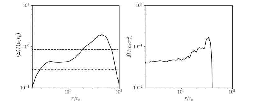
The left panel of Figure 2 shows the radial distribution of the azimuthally averaged surface density
| (16) |
averaged before including the radiation term (). The surface density is highest around . The density enhancement is the remnant of the initial torus. The right panel of Figure 2 shows the net mass accretion rate computed by;
| (17) |
where is the radial velocity in cylindrical coordinates. The net mass accretion rate is constant up to . The unit density is set so that this accretion rate is equal to the accretion rate specified as a parameter.
In this paper, numerical results for model M01 (, ), and model M03 (, ) are presented. Here, is the Eddington accretion rate defined by , where is the Eddington luminosity. Table 1 summarizes the normalizations and parameters used in this paper.
| Black hole mass | |
|---|---|
| Velocity | |
| Length | |
| Eddington Luminosity | |
| Eddington accretion rate |
| M01 | M03 | |
|---|---|---|
| Density | ||
| Energy and Pressure | ||
| Flux | ||
| Magnetic field |
The horizontal lines in the left panel of Figure 2 show the surface density corresponding to for Model M01 and M03, where is the electron scattering optical depth calculated by
| (18) |
For model M01, exceeds in the region . In model M03, exceeds in .
3 Numerical results
3.1 Formation of the Soft X-ray Emitting, Warm Comptonization Region
Figure 3 shows the time evolution of the azimuthally averaged surface density (upper panels) and the density-weighted azimuthally averaged equatorial temperature (lower panels) for model M01 (left panels) and M03 (right panels). After the inclusion of the radiative cooling term at , the accretion flow quickly cools and warm disk with temperature is formed at in M01 and cool dense disk with temperature is formed at in M03.
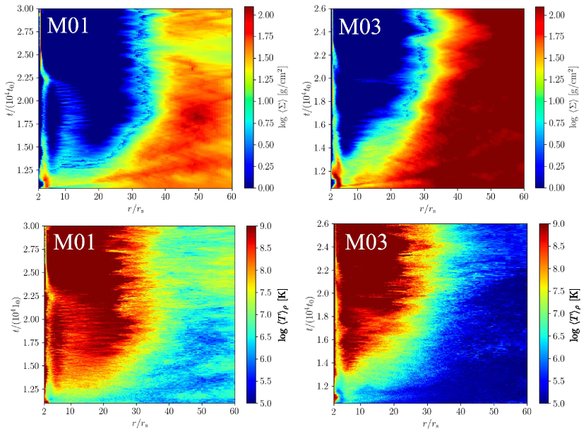
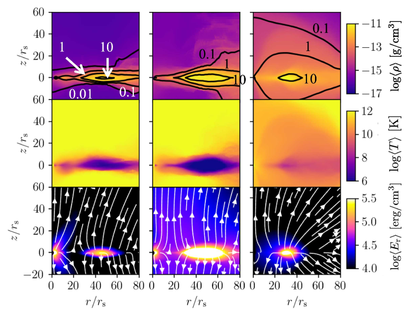
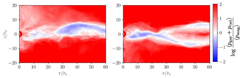
Figure 4 shows the azimuthally averaged density (top), temperature (middle), and radiation energy density (bottom) distributions when the warm disk is formed. The left panels are for model M01 averaged over , and the middle panels are for model M03 averaged over . The right panel shows results without Compton cooling/heating reported by Igarashi et al. (2020) (model NC, , ). The contours in the top panels of Figure 4 show isocontours of . In the model with Comptonization, the disk thickness and temperature decrease due to Compton cooling. In the outer region (), the gas temperature decreases significantly to K in model M01 and K in model M03, and a warm, Thomson-thick region is formed. In models M01 and M03, the radiation energy density in the warm region is large. In the region where , radiation is trapped in this region and the region is radially wider than in the model without Comptonization. The radiation energy density in model M01 is comparable to that in model NC. On the other hand, model M03 has a higher radiation energy density than the other models due to the larger optical depth in the warm region. The white streamlines in the bottom panels show the direction of the radiative flux in the poloidal plane. The direction of the radiative flux is almost vertical in the region where .
The bolometric luminosity of Model M01 is , consistent with the X-ray intensity at the onset of the changing look state transition. The luminosity increases with increasing the mass accretion rate, reaching in model M03. This luminosity is consistent with that in the UV and soft X-ray dominant state of CLAGN.
To identify the soft X-ray emitting region, we calculate the Compton -parameter defined by
| (19) |
When , is set equal to , as discussed in the previous section. As we also mentioned in Section 2, we set the lower limit of temperature as to avoid the negative gas pressure in the simulation. This can lead to the overestimation of the Compton -parameter. To avoid this, we replace the electron temperature with radiation temperature in the region where when we compute the Compton -parameter. Since can be less than , our estimate gives a lower limit of the Compton -parameter. Figure 5 shows the radial distribution of density-weighted azimuthally averaged (black dotted curves) and the Compton -parameter (blue solid curves). In model M01, the warm region with a temperature lies outside . The Compton -parameter in this region is . The CLAGN observation suggests that the Compton -parameter of the soft X-ray emitting region is and less than (Noda & Done, 2018; Tripathi & Dewangan, 2022). This is consistent with our simulation results. The Compton -parameter for M01 is in the hot inner region () where K. The hard X-rays can be emitted from this region by inverse Compton scattering of soft photons. In M03, the warm region () moves inward and is located around . The Compton -parameter in this warm region is , so we expect soft X-ray emission from this region. In the outer region where , since the electron temperature drops to K, we expect UV emission from this region.
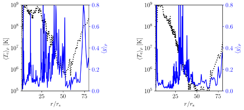
Table 2 summarizes the observational features of our simulations. In model M01, the soft X-ray emitting region appears around but the UV emitting region does not appear because the temperature exceeds K. In model M03, temperature in decreases down to K (see figure 5) and emits UV radiation. In model NC, the Compton -parameter is larger but the temperature exceeds K because Compton cooling is not included (Igarashi et al., 2020).
| Model | Disk Luminosity | Soft X-ray emitting region | UV emitting region | Compton- in the warm region |
| M01 | Yes | No | ||
| M03 | Yes | Yes | ||
| NC | Yes | No |
Figure 6 shows the distribution of for model M01 (left) and M03 (right), where is the radiation pressure. In M01, the magnetic pressure is dominant in the warm region in the upper half-hemisphere and in the hot inner torus. In model M03, the magnetic pressure dominates in the inner torus and in the warm region (). The radiation pressure dominates in the outer region For M01, the accretion rate is around % of the Eddington accretion rate, and the radiation pressure is lower than that in model NC (without Comptonization) reported in Igarashi et al. (2020). This is because the disk temperature in M01 is lower than that in NC due to Compton cooling.
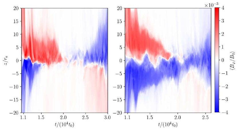
In model M01, the magnetic pressure dominant warm region appears only above the equatorial plane because the azimuthal magnetic fields below the equatorial plane reconnect with those above the equatorial plane. Figure 7 shows the butterfly diagram of the azimuthally averaged azimuthal magnetic fields at . During the vertical contraction of the disk due to radiative cooling, azimuthal magnetic fields anti-symmetric to the equatorial plane reconnect, and in model M01, only positive (red) magnetic fields remain in the upper hemisphere. This is the reason why the magnetic pressure dominant region in figure 6 appears only in the upper hemisphere around . In the later stage (), the azimuthal magnetic fields are again amplified by magnetorotational instability, and their polarity reverses. In model M03, azimuthal magnetic fields remain both in the lower and upper hemispheres at .
3.2 Heating by the Magnetic Reconnection around the Equatorial Plane
Figure 8 shows the time variation of the azimuthally averaged vertically integrated magnetic pressure (blue solid line), and the density-weighted azimuthally averaged equatorial temperature (black dashed line) for model M01 at . Around and , the magnetic pressure decreases, and the equatorial temperature increases. It indicates that magnetic energy is converted to thermal energy.
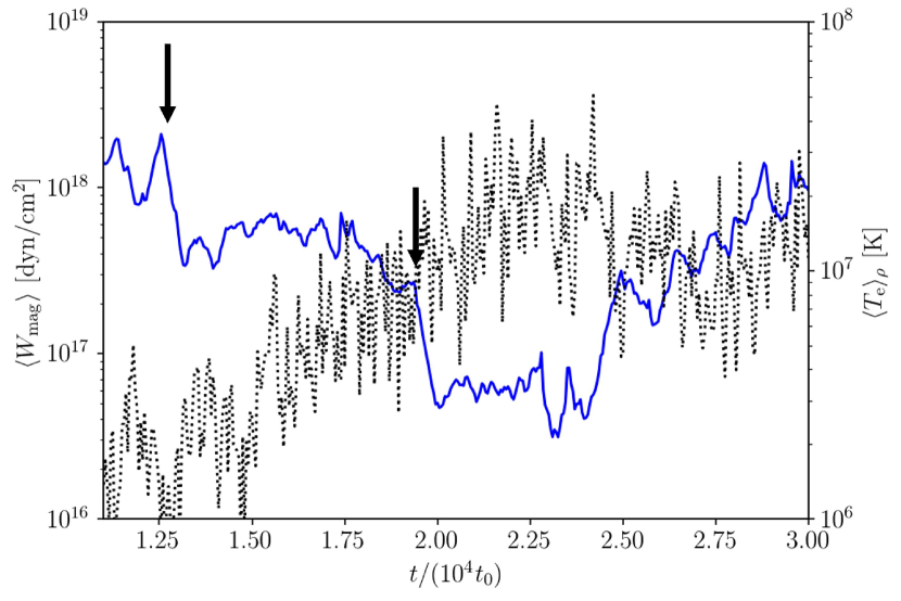
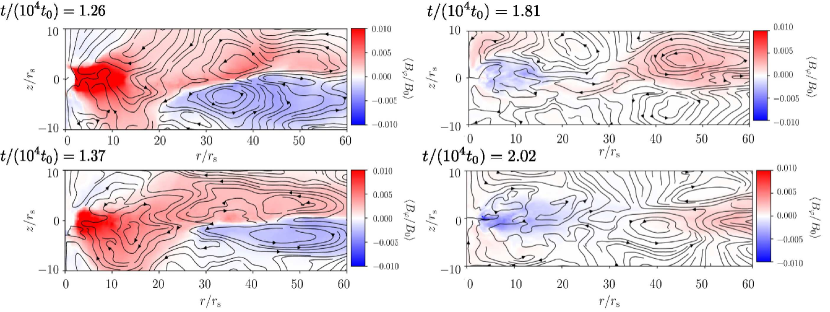
Figure 9 shows the azimuthally averaged azimuthal magnetic field and poloidal magnetic field lines before and after (left panels) and (right panels). In the left panels, azimuthal magnetic flux tubes with opposite poloidal and azimuthal magnetic fields are moving outward. These helical flux tubes are formed in the inner region () at around . They collide at the equatorial plane and merge. This event is similar to the merging of two spheromacs with opposite current helicity . The merging of the counter-helicity flux tubes converts the magnetic energy into thermal energy and heats the plasma (Ono et al., 1996). The right panels of figure 9 show that the azimuthal magnetic field in the inner hot flow () is reversed from that in the left panels and magnetic reconnection with that in the outer warm disk takes place.
The outward motion of the helical flux tubes produces the outward motion of the plasma in the equatorial region. Figure 10 shows the space-time plot of the accretion rate at (left panel), (middle panel), and the net mass accretion rate (right panel) for M01. Before the radiative cooling is included (), accretion proceeds in the equatorial region of the disk but as the disk cools, accretion takes place mainly in the surface region of the disk, and outward motion becomes prominent in the equatorial region. It indicates that meridional circulation is taking place in the radiatively cooled warm disk at . The surface accretion flow is driven by the angular momentum loss of the plasma around the disk surface through large-scale poloidal magnetic fields threading the disk. The surface accretion flow was called ’avalanche flow’ in Matsumoto et al. (1996).
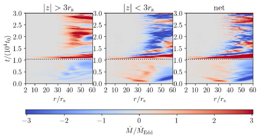
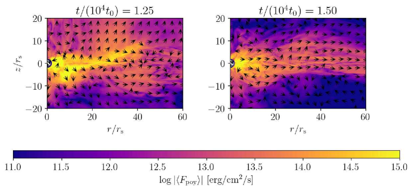
Figure 11 shows the distribution of the Poynting flux at (left), and (right). In the warm region at , radially outward Poynting flux is comparable to the radiative flux in this region. It indicates that the magnetic energy transported to this region contributes to the heating of the plasma. Heating of the accretion flow by Poynting flux from the inner region has been studied by general relativistic radiation MHD simulations by Takahashi et al. (2016). Our numerical results indicate that the Poynting flux contributes to the heating of the warm Compton region of the disk even when the central black hole is not rotating.
4 Comparison with Models of Magnetized Disks
We showed by radiation MHD simulations including Compton cooling/heating that the warm Comptonization region supported by azimuthal magnetic fields is formed in the region outside the radiatively inefficient accretion flow near the black hole. In this region, the disk shrinks in the vertical direction by radiative cooling. In this section, we compare numerical results with steady models of magnetized black hole accretion flows. The basic equations of steady accretion disks partially supported by the magnetic pressure of the azimuthal magnetic field were derived by Oda et al. (2009) assuming that the heating term in the energy equation is computed by using where is the angular speed of the rotating disk, and is the vertically integrated total pressure . Here we update their model by including additional magnetic heating due to magnetic reconnection and assume that . The derivation of thermal equilibrium curves for this model is shown in Appendix. In this section, we compare the numerical results with the magnetized disk model.
Here, we examine the angular momentum transport rate, which is calculated by the following equation.
| (20) |
Figure 12 shows the time evolution of averaged in . The dashed curve shows in the equatorial region where , and the solid curve shows in the surface region where . The value calculated in the surface region (solid curve) is larger than that of the disk region. The smaller in the equatorial region is due to the inhibition of accretion through the radially outward motion of helical flux tubes. In the following, we adopt .
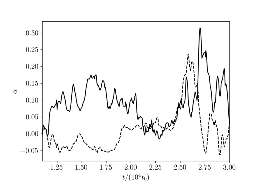
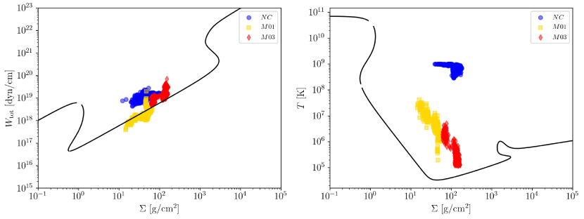
Figure 13 over plots numerical results and the thermal equilibrium curve when , and . Here, is the azimuthal magnetic flux, and is a parameter that relates the magnetic flux and surface density as (see Appendix). The yellow rectangles and red diamonds show the surface density and the vertically integrated total pressure for model M01 and model M03 at . The blue circles are for model NC at
Our simulation results are located between the optically thin branch and the optically thick branch. This is similar to the results for stellar-mass black holes (Machida et al., 2006; Dexter et al., 2021). In model NC (blue circles), is larger than the equilibrium solution because Compton cooling is neglected in this model, and the bremsstrahlung cooling time scale is much longer than the dynamical time scale.
In model M01 (yellow rectangles), the total pressure decreases towards the magnetic pressure-supported disk solution. The disk contraction enhances the magnetic pressure in the cool region and maintains the disk with a luminosity of around .
In model M03 (red diamonds in Figure 13), the large optical depth for Thomson scattering enhances the radiation pressure so that the vertically integrated total pressure exceeds that of the magnetic pressure-dominant disk.
The right panel of Figure 13 shows the thermal equilibrium curves in the surface density and temperature planes. The yellow rectangles and red diamonds show the azimuthally averaged surface density and temperature at for model M01 and model M03 at and the blue circles are for model NC at , respectively. Our numerical results indicate that the temperature is K at . This is consistent with the observation of the soft X-ray emission in CLAGN. However, the temperature is higher than that in the equilibrium solutions. The higher temperature can be explained by the additional heating due to the dissipation of magnetic energy caused by the merging of the antiparallel azimuthal magnetic field near the equatorial plane.
The additional heating through the injection of the Poynting flux from the inner region can be evaluated by where is the radius where the outward moving helical flux tubes are formed. Since , is proportional to when is fixed. Thus, at , . When we denote , . The heating rate is . When we adopt as suggested by figure 9, .
Figure 14 shows the thermal equilibrium curves in surface density and vertically integrated total pressure (left panel) and temperature (right panel) for and . The yellow rectangles, red diamonds, and blue circles show the numerical results. In the left panel of Figure 14, the magnetic pressure-supported equilibrium solution does not change with , because the gas pressure does not contribute to the total pressure in this branch (plasma in this regime). On the other hand, since the gas temperature increases with the additional heating , the thermal equilibrium curve for the surface density and temperature approaches the numerical results when .
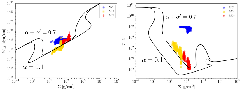
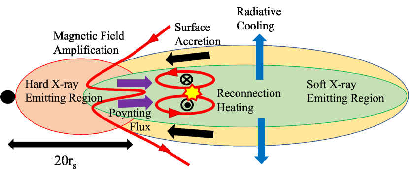
Figure 15 schematically shows the energy transport in the warm region suggested by numerical results. Magnetic field amplification through the surface accretion converts the gravitational energy to the magnetic energy around the interface between the radiatively cooled disk and the inner hot RIAF and forms helical azimuthal magnetic flux tubes. The helical flux tubes are expelled from the region through Lorentz force toward the positive radial direction and transport the magnetic energy. The magnetic energy transported to the warm disk is converted to thermal energy through magnetic reconnection.
It should be noted that the magnetic energy has been accumulated in the disk by mass accretion which releases the gravitational energy. Therefore, the time-averaged heating rate should be determined by the time-averaged accretion rate. However, there can be a time lag between the magnetic energy accumulation and the dissipation. Therefore, there can be a transient state in which the energy dissipation rate is larger than that expected from the accretion rate at that state. When the magnetic energy release ceases, the cooling will dominate heating, so that the disk will shrink in the vertical direction, which enhances the vertically integrated magnetic energy again.
5 Summary
In this paper, we have shown the results of the global three-dimensional radiation MHD simulations with the sub-Eddington accretion rate. The simulations successfully reproduced the soft X-ray emitting Thomson-thick warm Comptonization region with .
When the accretion rate is (model M01), a warm, Thomson-thick region with an average temperature of K is formed outside . In this state, the magnetic pressure is dominant in the warm region. The bolometric luminosity is close to the dark phase of the CLAGN. As the mass accretion rate increases (model M03), the warm region is formed around , and the temperature of the cool outer region decreases to K. In this state, the cool region () is mainly dominated by radiation pressure, because the optical depth is larger than that in model M01. The luminosity is , which is close to the luminous phase of the CLAGN. The temperature and the Thomson optical depth of the warm region are consistent with the observational property of the warm Comptonization region in CLAGN (Noda & Done, 2018; Tripathi & Dewangan, 2022). As the radiation pressure increases further, the radiative cooling rate increases, and the UV-emitting cold region forms which is also consistent with increased UV emission in the luminous state of CLAGN (Noda & Done, 2018; Tripathi & Dewangan, 2022). We should note that the warm region is optically thin for the effective optical depth for model M01. Therefore, soft X-ray emission from reflections of cold disks is ruled out, at least in the low luminosity state. Soft X-rays are emitted from the warm Comptonization region itself by Comptonizing photons emitted by bremsstrahlung or synchrotron radiation in the same region, or by upscattering photons emitted from the outer cool region by inverse Compton scattering. In contrast, in model M03, the effective optical depth is close to unity in the region. In this region, soft X-rays can be emitted from the surface region (Kawanaka & Mineshige, 2023) as well as the warm Comptonization region near the equatorial plane around .
We have also obtained the thermal equilibrium solutions of magnetized disks with an azimuthal magnetic field for black holes. When the magnetic flux at exceeds Mx/cm, the equilibrium solutions with temperature K appear when . Numerical results show that the accretion flow approaches this state in the plane, but the temperature is an order of magnitude larger than the equilibrium solution unless additional heating is considered. The origin of the additional heating is the magnetic energy dissipated through the reconnection of reversed magnetic fields transported from the inner region.
| (1) |
and
| (2) |
where the subscript denotes the value at the equatorial plane, and are the disk half thickness, where , and are the total pressure, and Keplerian angular velocity, respectively. Integrating the equations in the vertical direction, the surface density and the vertically integrated total pressure can be written as
| (3) |
and
| (4) |
where . By rewriting and using and , we obtain
| (5) |
Now, assuming axisymmetry and integrating the azimuthally averaged equations in the vertical direction, we get:
| (6) |
| (7) |
| (8) |
where is the specific angular momentum and is the specific angular momentum carried into the black hole. The left-hand side of equation (8) is the advective cooling rate . We assume . Oda et al. (2009) assumed that the magnetic flux advection rate where is determined by . Here we modify the formulation by introducing a parameter and assume that
| (9) |
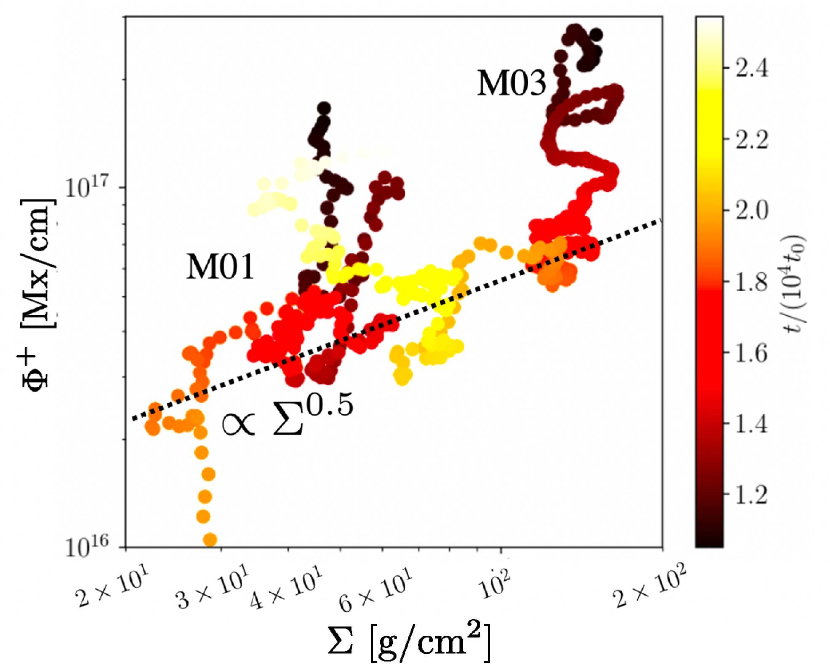
When , the magnetic flux is stored in the region where the mass accumulates. Here we should note that the magnetic flux is the magnetic flux integrated in the vertical direction. Thus the azimuthal magnetic field cancels when the azimuthal magnetic field is anti-symmetric with respect to the equatorial plane. Here we use to avoid cancellation of the azimuthal magnetic flux when is anti-symmetric with respect to the equatorial plane. Figure 16 shows the relation between the absolute magnetic flux and at obtained by radiation MHD simulations. The magnetic flux is larger in the early stage. In the later stage, the magnetic flux decreases, because the anti-symmetric azimuthal magnetic field dissipates around the equatorial plane. The azimuthal magnetic flux and the parameter can be estimated to be and , respectively.
We further assume that the disk heating rate is written as
| (10) |
Here, the first term on the right-hand side is the heating by the vertically integrated component of the stress tensor and the second term is the enhanced heating by magnetic reconnection, where is proportional to the reconnection rate.
For radiative cooling, we consider thermal bremsstrahlung emission. The cooling rate in the optically thin limit is written as
| (11) |
and the cooling rate in the optically thick limit is written as
| (12) |
where and are Stefan-Boltzmann constant and the total optical depth. Here is the absorption optical depth, and is the optical depth for Thomson scattering.
For the intermediate case, we use the approximate form of radiative cooling (e.g., Abramowicz et al., 1996),
| (13) |
where
| (14) |
We also consider the cooling by the inverse Compton scattering. The cooling rate by the inverse Compton scattering can be written as
| (15) |
where
| (16) |
is the radiation temperature. For simplicity, we assume that the ion and electron temperatures are the same. However, we should consider the temperature difference between ions and electrons in hot accretion flows where K. We can neglect the temperature difference between electrons and ions in the warm Comptonization region where K.
To obtain the thermal equilibrium curves of the black hole accretion flows, taking into account the azimuthal magnetic field we need to solve the equation of state and the balance between heating, radiative cooling, and advective cooling. Defining and , we obtain
| (17) |
and
| (18) |
The thermal equilibrium curve is obtained by solving for a given radius and mass accretion rate.
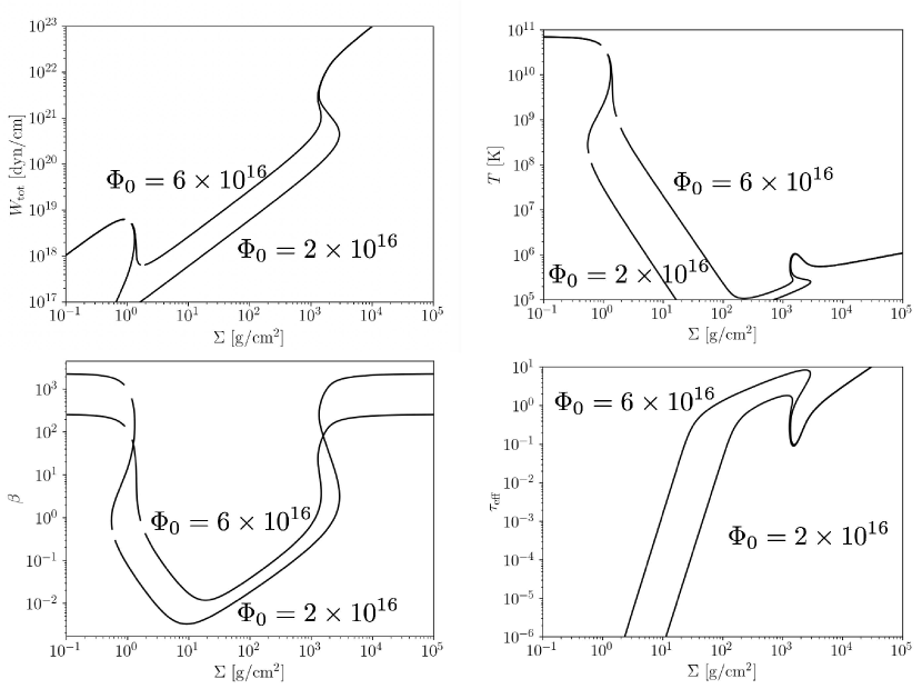
Figure 17 shows the result for a supermassive black hole with mass at when , , and . The upper left panel of Figure 17 shows the solution for the vertically integrated total pressure and surface density. When the surface density exceeds the upper limit for RIAF, the vertically integrated total pressure decreases because the radiative cooling overcomes the disk heating. However, since the magnetic pressure increases as the disk shrinks in the vertical direction, the enhanced heating balances the radiative cooling, so that the intermediate state between the optically thin branch and the optically thick standard disk appears as shown in Oda et al. (2009) for a stellar-mass black hole.
The upper right panel of figure 17 shows the thermal equilibrium curve in the surface density and planes. When the magnetic flux exceeds Mx/cm, a warm ( K) region appears when . The temperature and Thomson optical depth in this region are comparable to the warm Comptonization region and can explain the soft X-ray emission. Note that the temperature of this region is lower than that of stellar-mass black holes, where K (Oda et al., 2009, 2012).
The lower left panel of figure 17 shows the plasma defined as . In the intermediate state, the magnetic pressure dominates the gas and radiation pressure. Note that the plasma is lower for the lower magnetic flux model. This is because the disk heating rate can only balance the radiative cooling when the magnetic pressure is much higher than the gas pressure.
The bottom right panel shows that the warm Comptonization region is optically thin for the effective optical depth.
References
- Abramowicz et al. (1996) Abramowicz, M. A., Chen, X. M., Granath, M., & Lasota, J. P. 1996, ApJ, 471, 762, doi: 10.1086/178004
- Belloni & Motta (2016) Belloni, T. M., & Motta, S. E. 2016, in Astrophysics and Space Science Library, Vol. 440, Astrophysics of Black Holes: From Fundamental Aspects to Latest Developments, ed. C. Bambi, 61, doi: 10.1007/978-3-662-52859-4_2
- Dexter et al. (2021) Dexter, J., Scepi, N., & Begelman, M. C. 2021, ApJL, 919, L20, doi: 10.3847/2041-8213/ac2608
- Done et al. (2012) Done, C., Davis, S. W., Jin, C., Blaes, O., & Ward, M. 2012, MNRAS, 420, 1848, doi: 10.1111/j.1365-2966.2011.19779.x
- Done et al. (2007) Done, C., Gierliński, M., & Kubota, A. 2007, A&A Rev., 15, 1, doi: 10.1007/s00159-007-0006-1
- García et al. (2019) García, J. A., Kara, E., Walton, D., et al. 2019, ApJ, 871, 88, doi: 10.3847/1538-4357/aaf739
- Gierliński & Done (2004) Gierliński, M., & Done, C. 2004, MNRAS, 349, L7, doi: 10.1111/j.1365-2966.2004.07687.x
- Hawley & Balbus (2002) Hawley, J. F., & Balbus, S. A. 2002, ApJ, 573, 738, doi: 10.1086/340765
- Huang et al. (2023) Huang, J., Jiang, Y.-F., Feng, H., et al. 2023, ApJ, 945, 57, doi: 10.3847/1538-4357/acb6fc
- Ichimaru (1977) Ichimaru, S. 1977, ApJ, 214, 840, doi: 10.1086/155314
- Igarashi et al. (2020) Igarashi, T., Kato, Y., Takahashi, H. R., et al. 2020, ApJ, 902, 103, doi: 10.3847/1538-4357/abb592
- Jiang et al. (2019) Jiang, Y.-F., Blaes, O., Stone, J. M., & Davis, S. W. 2019, ApJ, 885, 144, doi: 10.3847/1538-4357/ab4a00
- Kato et al. (2004) Kato, Y., Mineshige, S., & Shibata, K. 2004, ApJ, 605, 307, doi: 10.1086/381234
- Kawanaka & Mineshige (2023) Kawanaka, N., & Mineshige, S. 2023, arXiv e-prints, arXiv:2304.07463, doi: 10.48550/arXiv.2304.07463
- Kawashima et al. (2009) Kawashima, T., Ohsuga, K., Mineshige, S., et al. 2009, PASJ, 61, 769, doi: 10.1093/pasj/61.4.769
- Kobayashi et al. (2018) Kobayashi, H., Ohsuga, K., Takahashi, H. R., et al. 2018, PASJ, 70, 22, doi: 10.1093/pasj/psx157
- Kubota & Done (2018) Kubota, A., & Done, C. 2018, MNRAS, 480, 1247, doi: 10.1093/mnras/sty1890
- Lančová et al. (2019) Lančová, D., Abarca, D., Kluźniak, W., et al. 2019, ApJL, 884, L37, doi: 10.3847/2041-8213/ab48f5
- Liska et al. (2022) Liska, M. T. P., Musoke, G., Tchekhovskoy, A., Porth, O., & Beloborodov, A. M. 2022, ApJ, 935, L1, doi: 10.3847/2041-8213/ac84db
- Lowrie et al. (1999) Lowrie, R. B., Morel, J. E., & Hittinger, J. A. 1999, ApJ, 521, 432, doi: 10.1086/307515
- Machida et al. (2006) Machida, M., Nakamura, K. E., & Matsumoto, R. 2006, PASJ, 58, 193, doi: 10.1093/pasj/58.1.193
- Magdziarz et al. (1998) Magdziarz, P., Blaes, O. M., Zdziarski, A. A., Johnson, W. N., & Smith, D. A. 1998, MNRAS, 301, 179, doi: 10.1046/j.1365-8711.1998.02015.x
- Matsumoto et al. (1996) Matsumoto, R., Uchida, Y., Hirose, S., et al. 1996, ApJ, 461, 115, doi: 10.1086/177041
- Matsumoto et al. (2019) Matsumoto, Y., Asahina, Y., Kudoh, Y., et al. 2019, PASJ, 71, 83, doi: 10.1093/pasj/psz064
- McClintock & Remillard (2006) McClintock, J. E., & Remillard, R. A. 2006, in Compact stellar X-ray sources, Vol. 39, 157–213, doi: 10.48550/arXiv.astro-ph/0306213
- Miyakawa et al. (2008) Miyakawa, T., Yamaoka, K., Homan, J., et al. 2008, PASJ, 60, 637, doi: 10.1093/pasj/60.3.637
- Motta et al. (2009) Motta, S., Belloni, T., & Homan, J. 2009, MNRAS, 400, 1603, doi: 10.1111/j.1365-2966.2009.15566.x
- Nakamura et al. (1997) Nakamura, K. E., Kusunose, M., Matsumoto, R., & Kato, S. 1997, PASJ, 49, 503, doi: 10.1093/pasj/49.4.503
- Narayan & Yi (1995) Narayan, R., & Yi, I. 1995, ApJ, 444, 231, doi: 10.1086/175599
- Noda & Done (2018) Noda, H., & Done, C. 2018, MNRAS, 480, 3898, doi: 10.1093/mnras/sty2032
- Oda et al. (2009) Oda, H., Machida, M., Nakamura, K. E., & Matsumoto, R. 2009, ApJ, 697, 16, doi: 10.1088/0004-637X/697/1/16
- Oda et al. (2012) Oda, H., Machida, M., Nakamura, K. E., Matsumoto, R., & Narayan, R. 2012, Publications of the Astronomical Society of Japan, 64, 15
- Oknyansky et al. (2020) Oknyansky, V. L., Winkler, H., Tsygankov, S. S., et al. 2020, MNRAS, 498, 718, doi: 10.1093/mnras/staa1552
- Ono et al. (1996) Ono, Y., Yamada, M., Akao, T., Tajima, T., & Matsumoto, R. 1996, Phys. Rev. Lett., 76, 3328, doi: 10.1103/PhysRevLett.76.3328
- Paczyńsky & Wiita (1980) Paczyńsky, B., & Wiita, P. J. 1980, A&A, 88, 23
- Padmanabhan (2000) Padmanabhan, P. 2000, Theoretical astrophysics. Vol.1: Astrophysical processes (Cambridge Univ. Press)
- Popović et al. (2023) Popović, L. Č., Ilić, D., Burenkov, A., et al. 2023, A&A, 675, A178, doi: 10.1051/0004-6361/202345949
- Remillard & McClintock (2006) Remillard, R. A., & McClintock, J. E. 2006, ARA&A, 44, 49, doi: 10.1146/annurev.astro.44.051905.092532
- Ricci & Trakhtenbrot (2023) Ricci, C., & Trakhtenbrot, B. 2023, Nature Astronomy, 7, 1282, doi: 10.1038/s41550-023-02108-4
- Ricci et al. (2020) Ricci, C., Kara, E., Loewenstein, M., et al. 2020, ApJ, 898, L1, doi: 10.3847/2041-8213/ab91a1
- Ricci et al. (2021) Ricci, C., Loewenstein, M., Kara, E., et al. 2021, ApJS, 255, 7, doi: 10.3847/1538-4365/abe94b
- Ryan et al. (2015) Ryan, B. R., Dolence, J. C., & Gammie, C. F. 2015, ApJ, 807, 31, doi: 10.1088/0004-637X/807/1/31
- Ryan et al. (2018) Ryan, B. R., Ressler, S. M., Dolence, J. C., Gammie, C., & Quataert, E. 2018, ApJ, 864, 126, doi: 10.3847/1538-4357/aad73a
- Ryan et al. (2017) Ryan, B. R., Ressler, S. M., Dolence, J. C., et al. 2017, ApJ, 844, L24, doi: 10.3847/2041-8213/aa8034
- Sadowski et al. (2017) Sadowski, A., Wielgus, M., Narayan, R., et al. 2017, MNRAS, 466, 705, doi: 10.1093/mnras/stw3116
- Shakura & Sunyaev (1973) Shakura, N. I., & Sunyaev, R. A. 1973, A&A, 24, 337
- Shapovalova et al. (2019) Shapovalova, A. I., Popović, , L. Č., et al. 2019, MNRAS, 485, 4790, doi: 10.1093/mnras/stz692
- Shappee et al. (2014) Shappee, B. J., Prieto, J. L., Grupe, D., et al. 2014, ApJ, 788, 48, doi: 10.1088/0004-637X/788/1/48
- Shidatsu et al. (2019) Shidatsu, M., Nakahira, S., Murata, K. L., et al. 2019, ApJ, 874, 183, doi: 10.3847/1538-4357/ab09ff
- Takahashi & Ohsuga (2013) Takahashi, H. R., & Ohsuga, K. 2013, ApJ, 772, 127, doi: 10.1088/0004-637X/772/2/127
- Takahashi et al. (2016) Takahashi, H. R., Ohsuga, K., Kawashima, T., & Sekiguchi, Y. 2016, ApJ, 826, 23, doi: 10.3847/0004-637X/826/1/23
- Takahashi et al. (2013) Takahashi, H. R., Ohsuga, K., Sekiguchi, Y., Inoue, T., & Tomida, K. 2013, ApJ, 764, 122, doi: 10.1088/0004-637X/764/2/122
- Tanaka & Shibazaki (1996) Tanaka, Y., & Shibazaki, N. 1996, ARA&A, 34, 607, doi: 10.1146/annurev.astro.34.1.607
- Tripathi & Dewangan (2022) Tripathi, P., & Dewangan, G. C. 2022, ApJ, 930, 117, doi: 10.3847/1538-4357/ac610f
- Yokoyama & Shibata (1994) Yokoyama, T., & Shibata, K. 1994, ApJ, 436, L197