Spatio-Temporal Graphical Counterfactuals:
An Overview

Abstract

Counterfactual thinking is a critical yet challenging topic for artificial intelligence to learn knowledge from data and ultimately improve their performances for new scenarios. Many research works, including Potential Outcome Model and Structural Causal Model, have been proposed to realize it. However, their modelings, theoretical foundations and application approaches are usually different. Moreover, there is a lack of graphical approach to infer spatio-temporal counterfactuals, that considers spatial and temporal interactions between multiple units. Thus, in this work, our aim is to investigate a survey to compare and discuss different counterfactual models, theories and approaches, and further build a unified graphical causal frameworks to infer the spatio-temporal counterfactuals.

I Introduction

How to enable an intelligent machine to think and answer a counterfactual question? E.g., sometimes we want to know, if a different investment strategy had been implemented, would we obtain higher returns? Or, in computer networks, what changes would occur in network load if a node’s configuration had never been changed? Or, would someone still purchase the product even if they had never been shown the advertisement? These questions generally have the counterfactual pattern, that is, “Observed $\dots$, if had done $\dots$, how would $\dots$ go?”. Thus, according to the pattern, firstly, time is necessary to consider, because the questions are queried now, but the counterfactual actions are supposed to be done in the past. Secondly, counterfactual outcomes are unobservable. The outcomes of some actions are observed if the actions have been done to the real-world system, thus these outcomes are factual. But the counterfactual outcomes are not observed, and they are imaged through supposing different actions had been done.

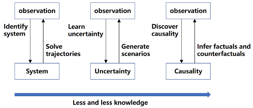
Figure 1: Infer counterfactuals with less and less knowledge.

To enable an intelligent machine to imitate counterfactual thinking like human, there are mainly three approaches, as shown in Fig. 1. The first is system identification, which aims to identify the system dynamics, and then solve the evolution trajectories with different initial values [1]. This process may be data-driven and adaptive, but the physical mechanisms and models are necessary to be known as knowledge in prior [2, 3, 4, 5]. E.g., in [6, 7], functional basis or network structure are necessary to be known at least one to identify the network dynamics sparsely. However, the knowledge of system mechanism is usually hard to obtain in prior.

The second approach is generative modeling, which aims to model and learn the system uncertainty, and then generate scenarios with different random inputs [8, 9]. Thus, compared with system identification, generative approach is not necessary to know the determined part, that is the knowledge of system mechanism, but on contrary, it focuses on the uncertain modeling, especially with the deep learning [10, 11, 12, 13, 14, 15]. However, the generated scenarios would not be out of the distribution of the observational data [9], while the counterfactual scenarios are usually not in the observational factuals. Thus, the mechanism knowledge is still needed to correct the bias between the distributions of factuals and counterfactuals.

Thus, the third approach is causal inference, which aims to discover causality from the observational data, and then infer factuals and counterfactuals directly with as little knowledge as possible [16, 17]. Causal counterfactual inference enables artificial intelligence to learn the knowledge from data, and ultimately improve their performances for new scenarios. To realize it, many research works have been proposed to infer counterfactuals, including the temporal cases [18, 19, 20, 21, 22, 23]. However, there are still two challenging but critical issues to address: (i) Most current inference approaches are built on the frameworks of Potential Outcome Model (POM) [17] or Structural Causal Model (SCM) [16, 24, 25, 26]. The goals of them are the same, but their foundations are different. This induces difficulty in discussing them in a unified framework. (ii) The two frameworks both cannot infer spatio-temporal counterfactuals, that considers spatial and temporal interactions between system units.

Thus, the main contributions of this work are as follows:

1. A survey is investigated to discuss the frameworks from POM to SCM, including their theoretical foundations and application approaches. This part is organized from Section II to Section IV.

2. A Forward Counterfactual Inference algorithm is designed here to recursively and autonomously infer counterfactuals through causal graphical languages. This part is presented as Algorithm 1 in Section IV-C.

3. An overview of the spatio-temporal graphical counterfactual framework is proposed to discuss Spatio-Temporal Bayesian Networks, its nonstationarity, and the relationship with complex networks. This part is organized in Section V.

II Potential Outcome Model

The counterfactuals are defined as the unobserved potential outcomes in POM, as shown in TABLE I. Here, $Y$ is the potential outcomes of the target variable. $T$ is treatment variable. $T=1$ represents being treated and $T=0$ represents being controlled, with a group of randomized control trials on $N$ units. $X$ represents covariates that have relationship with $Y$ and $T$, and are controlled for randomized trials. POM models the general process from causal estimands ($T$, $Y$ and $X$) to “Science” [27]. In this case, for different treatments $T$, only one potential outcome, $Y(1)$ or $Y(0)$, can be observed, and another one is unobserved, namely the counterfactual.

TABLE I: Data for POM example.

Units	Covariates	Potential outcomes		Treatment
$i$	$X$	$Y(1)$	$Y(0)$	$T$
1	$x_{1}$	$y_{1}(1)$	$?$	$1$
2	$x_{2}$	$?$	$y_{2}(0)$	$0$
3	$x_{3}$	$?$	$y_{3}(0)$	$0$
4	$x_{4}$	$y_{4}(1)$	$?$	$1$
5	$x_{5}$	$y_{5}(1)$	$?$	$1$
$\vdots$	$\vdots$	$\vdots$	$\vdots$	$\vdots$
$N$	$x_{N}$	$?$	$y_{N}(0)$	$0$

II-A Inferring Counterfactuals through POM

To infer the counterfactuals through POM, one common approach is matching, e.g., exact matching. For a unit $i$, one can search the samples with exactly matching covariates $X$ but treatment $T$ is different, and then estimate the counterfactual outcome $Y_{i}(1-T_{i})$. But it is difficult to conduct if the dimension of $X$ is high, that requires large number of samples to support the matching. Thus, approximate matching is commonly better, e.g., caliper matching [28, 29, 30, 31] and propensity score matching [32, 33, 34, 35]. They approximately search a group of similar samples for the target unit with one or multiple measurements, and finally calculate the counterfactuals.

Another common approach is data-driven imputation, that views the counterfactuals as missing values, and interpolates them by fitting the observational data. To realize it, linear or nonlinear regressions [36, 37, 38, 39] are commonly used to interpolate the missing values from the trained regressive models on the observational data. Different from this, tensor decomposition approaches [40, 41, 42] recover the missing values by decomposing and reconstructing the sparse data tensor. Moreover, deep generative models [10, 11, 12, 13, 14, 15] are also used to model the uncertainty in data, and generate the missing values by randomly sampling. Note that, the generated missing values are not unique, but a group of values conforming to a random distribution. This is different compared to the regressive approaches and tensor decomposition approaches.

II-B Foundational Assumptions of POM

Before using the above approaches on the framework of POM, four assumptions are necessary to be accepted. The first is the stable unit treatment value assumption (SUTVA), defined as

Assumption 1 (SUTVA [43]).

In TABLE I,

1. there is no interference between units, that is, neither $Y_{i}(1)$ nor $Y_{i}(0)$ is affected by what action any other unit received.

2. there is no hidden versions of treatments, that is, no matter how unit $i$ received treatment $T=1$, the outcome that would be observed would be $Y_{i}(1)$, and similarly for treatment $T=0$.

SUTVA guarantees the identical independence between the experimental units, and for unit $i$, the outcome $Y_{i}$ is only up to its treatment $T_{i}$, not the others’. However, this assumption is not always satisfied, e.g., in the case of social network, in which there are frequent interactions between units with varying time.

The second assumption is consistency, defined as

Assumption 2 (Consistency [44, 45]).

In TABLE I, if the $i$-th unit is selected for a treatment $T_{i}$, the observed value of $Y_{i}$, neither $Y_{i}(1)$ nor $Y_{i}(0)$, is the same for all assignments of treatments to the other experimental units.

Another form to describe the consistency assumption through expectation $\mathbb{E}[\cdot]$ is

$$\mathbb{E}[Y(1)|T=1]=\sum_{i=1}^{N}y_{i}\times t_{i}=\mathbb{E}[Y|T=1],$$ (1)

$$\mathbb{E}[Y(0)|T=0]=\sum_{i=1}^{N}y_{i}\times(1-t_{i})=\mathbb{E}[Y|T=0],$$

where $y_{1},\dots,y_{N}$ are the samples for $N$ units, and $t_{1},\dots,t_{N}\in\{0,1\}$ are the values of treatment variable $T$, as shown in TABLE I. This is the same to the case of conditional expectation with $X$. Thus, the consistency assumption guarantees the missing counterfactual values in Section II-A can be interpolated by the other observational values actually.

The third assumption is positivity, defined as

Assumption 3 (Positivity [32]).

In TABLE I, $0<P(T=1|X=x)<1$.

This means for $X=x$, there are always some treatments randomly assigned with $T=0$ and $T=1$. Otherwise, the counterfactuals for $T=1$ could not be obtained if all units with $X=x$ are assigned with $T=0$, and this is the same to the counterfactuals for $T=0$.

The forth assumption is ignorability, defined as

Assumption 4 (Ignorability [44, 45]).

In TABLE I, $T{\perp\!\!\!\perp}Y(1),Y(0)|X$ for each unit.

Thus, the ignorability assumption implies that all the confounders have been observed in $X$, that is, no hidden confounder would interfere the observations of $Y(1),Y(0)$. Thus, the ignorability assumption is also called as unconfoundedness. This assumption are usually made to avoid the preference on experimental manipulation, that would guarantee the randomization in the experiments [46].

III Structural Causal Model

An SCM is built on a set of variables, including endogenous variables $\mathbf{V}=\{X_{1},\dots,X_{n}\}$ and exogenous variables $\mathbf{U}=\{U_{1},\dots,U_{n}\}$. Note that, endogenous variables are observable from data, but exogenous variables are not. Moreover, a set of functions $\mathbf{F}=\{f_{1},\dots,f_{n}\}$ are also set to describe the functional relationship between these variables.

For example, as shown in Fig. 2, the SCM can be functionally described as

$$f_{1}: X_{1}=U_{1},$$ (2)

$$f_{2}: X_{2}=aX_{1}+U_{2},$$

$$f_{3}: X_{3}=bX_{1}+cX_{2}+U_{3},$$

where $a=0.5,b=0.7,c=0.4$. $U_{1},U_{2},U_{3}$ are all additive noise, and they are mutually independent.

Note that, in an SCM, the functional relationship must conform to a directed-acyclic graphical constraint. The graph is early originated from the concept of Bayesian network [47, 48, 49, 50, 51]. And latter, it is also called as causal graphical model to highlight the causality [52, 53, 54, 16, 24]. And recently, it is also called as causal network in the field of causal discovery [55, 56, 57, 58, 59]. But actually, they are the same in the framework of SCM, and they are all directed acyclic graph (DAG) that represents Markovian knowledge. Thus, to avoid misunderstanding, we here use the name of Bayesian network uniformly, due to the fact that causal graphical model and causal network are not always a Bayesian network in Fig. 2. For example, Direct Cyclic Graph [60, 61, 62, 63], Markov network [64, 65], and Full Time Graph [25], they are also causal graph or causal network.

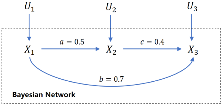
Figure 2: An example of SCM [24].

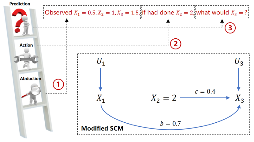
Figure 3: A diagram of Pearl’s causal ladder [24].

III-A Pearl’s Causal Ladder [16, 24, 26]

To infer the counterfactuals through SCM, there are three steps:

1. Abduction: Infer the values of exogenous variables $\mathbf{U}$ from the observational data;

2. Action: Perform an intervention on SCM, e.g., $do(X_{2}=2)$ on SCM in Fig. 2, and then, $X_{2}$ would be assigned with value $2$, and the arrows to $X_{2}$ would be modified, as shown in Fig. 3;

3. Prediction: Use the modified SCM to recalculate the counterfactuals of the target variable.

As shown in Fig. 3, we query “observed $X_{1}=0.5,X_{2}=1,X_{3}=1.5$, if had done $X_{2}=2$, what would $X_{3}=?$”. Obviously, this is a counterfactual question. Thus, follow the Pearl’s causal ladder, as shown in Fig. 3, we first infer the values of exogenous variables $\mathbf{U}=\{U_{1},U_{2},U_{3}\}$ from the observational data $X_{1}=0.5,X_{2}=1,X_{3}=1.5$, as follows:

$$U_{1} =0.5,$$ (3)

$$U_{2} =1-0.5\times 0.5=0.75,$$

$$U_{3} =1.5-0.7\times 0.5-0.4\times 1=0.75.$$

Then, $do(X_{2}=2)$ to obtain a modified SCM. And finally, recalculate the counterfactual of $X_{3}$, that is,

$$X_{3}(do(X_{2}=2))=0.5\times 0.7+2\times 0.4+0.75=1.9,$$ (4)

where $X_{3}(do(X_{2}=2))$ is different compared to the observational $X_{3}$.

The intervention, also named as $do$-operator [16], can be generalized into the form of probability, if modularity assumption is introduced as follow:

Assumption 5 (Modularity [16]).

If a set of variables $\{X_{j_{1}},\dots,X_{j_{p}}\}\subset\mathbf{V}$ is intervened, then for each variable $X\in\mathbf{V}$, it is obtained that

1. if $X\notin\{X_{j_{1}},\dots,X_{j_{p}}\}$, then $P(X|\mathbf{Pa}(X))$ remains unchanged. Here, $\mathbf{Pa}(X)$ is the predecessors of $X$ in Bayesian network, that is also called as causal parents.

2. if $X\in\{X_{j_{1}},\dots,X_{j_{p}}\}$, then $P(X=x|\mathbf{Pa}(X))=1$ if $x$ is the value set by intervention to $X$, otherwise, $P(X=x|\mathbf{Pa}(X))=0$.
   

This means, if a group of interventions are conducted on $X_{j_{1}},\dots,X_{j_{p}}$, the values of them would be fixed. The connections between them and their causal parents would be broken, and their causal parents would not affect them anymore in the modified SCM, just like in Fig. 3. Moreover, this also means that the probability distributions of the other variables that are not be intervened would not change.

III-B Foundational Assumptions of Bayesian Network

As presented above, to clearly define the causality, every SCM is associate to a Bayesian network with directed-acyclic graphical constraint. Thus, the causality in Bayesian network determines the counterfactuals foundationally. Thus, we discuss the foundational assumptions of Bayesian network in the following contents.

First of all, a concept of d-separation can be defined on a Bayesian network $\mathcal{G}$ as

Definition 1 (d-separation [47, 48, 49, 50, 51]).

Let $\mathbf{X}$, $\mathbf{Y}$ and $\mathbf{Z}$ be three disjoint subsets of endogenous variables $\mathbf{V}=\{X_{1},\dots,X_{n}\}$, and let $\mathbf{p}$ be any path from a node in $\mathbf{X}$ to a node in $\mathbf{Y}$ regardless of direction. $\mathbf{Z}$ is said to block $\mathbf{p}$ if and only if there is a node $v\in\mathbf{p}$ satisfying one of the following items:

1. $v$ has v-structure (two nodes $a,b\in\mathbf{p}$ pointing to $v$, namely $a\rightarrow v\leftarrow b$), and neither $v$ nor its any descendants are in $\mathbf{Z}$;

2. $v$ in $\mathbf{Z}$ and $v$ does not have v-structure.

Then, $\mathbf{Z}$ d-separate $\mathbf{X}$ and $\mathbf{Y}$, denoted as $\mathbf{X}{\perp\!\!\!\perp}_{\mathcal{G}}\mathbf{Y}|\mathbf{Z}$, if $\mathbf{Z}$ blocks any $\mathbf{p}$.

Then, two assumptions, causal Markov (or Markov property) and faithfulness, are introduced as follows:

Assumption 6 (Causal Markov [47, 48, 49, 50, 51]).

Probability distribution $P$ is Markovian to a Bayesian network $\mathcal{G}$ if

$$\mathbf{X}{\perp\!\!\!\perp}_{\mathcal{G}}\mathbf{Y}|\mathbf{Z}\Rightarrow\mathbf{X}{\perp\!\!\!\perp}\mathbf{Y}|\mathbf{Z},$$ (5)

where $\mathbf{X}$, $\mathbf{Y}$ and $\mathbf{Z}$ are three disjoint subsets.

Assumption 7 (Faithfulness [47, 48, 49, 50, 51]).

Probability distribution $P$ is faithful to a Bayesian network $\mathcal{G}$ if

$$\mathbf{X}{\perp\!\!\!\perp}\mathbf{Y}|\mathbf{Z}\Rightarrow\mathbf{X}{\perp\!\!\!\perp}_{\mathcal{G}}\mathbf{Y}|\mathbf{Z}$$ (6)

for all disjoint subsets $\mathbf{X}$, $\mathbf{Y}$ and $\mathbf{Z}$.

It is intuitive to understand the two assumptions, that is, the Bayesian network $\mathcal{G}$ has one-to-one correspondence to the independence of probability distribution $P$ in observational data. Thus, if they are satisfied, the joint distribution can be factorized according to the Bayesian network, as follow:

$$P(X_{1},\dots,X_{n})=\prod_{i=1}^{n}P(X_{i}|\mathbf{Pa}(X_{i})),$$ (7)

where $\mathbf{Pa}(X_{i})$ is the predecessors of $X_{i}$ in $\mathcal{G}$, that is also called as causal parents.

Moreover, a Bayesian network is also assumed to be causally sufficient, that is

Assumption 8 (Causal Sufficiency [47, 48, 49, 50, 51]).

Variables $\mathbf{V}$ are said to satisfy causal sufficiency if there is no hidden variable that is a common cause of two or more variables in $\mathbf{V}$.

This means, if a Bayesian network (or an SCM) is causally sufficient, there is no hidden path connecting two endogenous variables in $\mathbf{V}$, and all variable information is collected sufficiently to support the network. Actually, the ignorability assumption in POM (see Assumption 4) also implies the causal sufficiency, and this assumption is weaker than ignorability. But note that, the causal sufficiency is hard to satisfy practically, because many real-world systems (e.g., economic system and climate system) are complex, thus, we could not collect all the information to describe the systems usually. Thus, some research works focus on this issue. For example, FCI (or Fast Causal Inference) algorithm and its variants [66, 67, 68, 69, 70, 71] are proposed to discover causality in the presence of hidden variables. And some other related works [72, 73, 74] investigate the causal discovery with soft intervention, that intervenes the SCM but does not change the network structure. There are also some related works [75, 76, 77, 78] proposed approaches to search the optimal and efficient adjustment set, that all its variables are observable, minimal and valid, and the removal of any of its variables would destroys the validity.

IV Differences between POM and SCM

Through the above comparisons between POM and SCM, one can find many differences intuitively. For example, they have different statements for counterfactuals, even if some of them can be equally transformed for each other. Moreover, SCM has a causal graph to represent the causations, and the interventions are also introduced to modify the graph to obtain the counterfactuals, but POM does not use it. However, although they have made many distinctions to distinguish each other, as stated in Rubin’s and Pearl’s books [17, 26], there are still some fundamental differences and relationship that need to be discussed.

IV-A Ignorability and Back-door Criterion

In the view of statistics, the ignorability assumption (see Assumption 4) is equivalent in calculation to the causal sufficiency assumption (see Assumption 8) with a back-door criterion. The accurate definition of back-door criterion can be found in these papers and books [53, 54, 16, 24]. Here we present another from with respect to the TABLE I, defined as

Definition 2 (Back-door Criterion [53, 54, 16, 24]).

In TABLE I, the covariate $X$ is said to satisfy back-door criterion, if a Bayesian network is built on all the variables relative to $X,Y,T$, and there is an ordered pair $T\rightarrow Y$ that satisfy

1. no variable in $X$ is a descendant of $T$;

2. $X$ blocks every path between $T$ and $Y$ that contains an arrow into $T$.

Thus, for $X,Y,T$, only one structure can satisfy the back-door criterion, as shown in Fig. 4. And in the back-door path, it is obtained that

$$P(Y|do(T=1))$$ (8)

$$= \sum_{x}P(Y|do(T=1),X=x)P(X=x|do(T=1))$$

$$= \sum_{x}P(Y|T=1,X=x)P(X=x),$$

which is the same in case of $do(T=0)$ [53, 54, 16, 24]. Then, if the causal sufficiency is satisfied, that is, no hidden variable can interfere $X,Y,T$, the expectation of potential outcomes in TABLE I can be calculated by

$$\mathbb{E}[Y|do(T=1)]$$ (9)

$$= \sum_{y}y\times P(Y=y|do(T=1))$$

$$= \sum_{y}\sum_{x}y\times P(Y=y|T=1,X=x)P(X=x)$$

$$= \sum_{x}P(X=x)\sum_{y}y\times P(Y=y|T=1,X=x)$$

$$= \mathbb{E}[\mathbb{E}[Y|T=1,X]].$$

This is the same in POM, as follow:

$$\mathbb{E}[Y(1)]$$ (10)

$$= \mathbb{E}[\mathbb{E}[Y(1)|X]] /*Law~{}of~{}full~{}expectation*/$$

$$= \mathbb{E}[\mathbb{E}[Y(1)|T=1,X]] /*Ignorability*/$$

$$= \mathbb{E}[\mathbb{E}[Y|T=1,X]], /*Consistency*/$$

which is the same in case of $do(T=0)$. Thus, with comparing Eq. (9) and Eq. (10), $\mathbb{E}[Y|do(T=1)]=\mathbb{E}[Y(1)]$, and $\mathbb{E}[Y|do(T=0)]=\mathbb{E}[Y(0)]$, in the two frameworks, but they start from different assumptions. Thus, the ignorability assumption can be decomposed as the causal sufficiency assumption and the back-door criterion, and the causal sufficiency is relatively trivial to satisfy. Actually, the ignorability is more likely to be a technical assumption, that needs many controlled trials to deconfound, while the back-door path is clear to search in a Bayesian network. A potential and more difficult technical issue is to discover the network structure accurately.

IV-B Counterfactual Falsifiability

Back to the example in Fig. 3, if we query to a POM, “Observed $X_{1}=0.5,X_{2}=1,X_{3}=1.5$, if had done $X_{2}=2$, what would $X_{3}=?$”, we must ensure there are at least two observational samples, and they have the same values $X_{1}=0.5$ but different values in $X_{2}$. That is, one is $X_{2}=1$, and another one is $X_{2}=2$, to satisfy the positivity assumption (see Assumption 3). And then, due to the consistency assumption (see Assumption 2), we can infer the counterfactuals through matching the two samples exactly. But this is different in SCM, we can infer the counterfactuals through the Pearl’s causal ladder, even if we only have a single sample, as shown in Section III-A. Thus, how to falsify the counterfactuals?

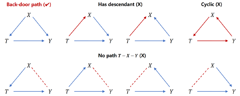
Figure 4: A diagram of back-door path.

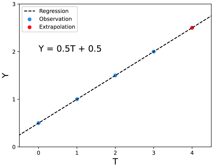
Figure 5: A diagram of data extrapolation.

It is a difficult question, because the counterfactuals are unobserved according to the definition (see “?” in TABLE I), and we need at least two samples for comparison. In general, we cannot back to the past to falsify it with a different treatment, and we cannot reproduce the same experiments completely at different times. Thus, the inferred counterfactuals in SCM cannot be falsified without the assumptions of positivity and consistency, and this view is rejected ambiguously in Pearl’s book [26].

Another explanation is that, without the positivity, but with the consistency only in POM, the counterfactuals can be extrapolated by regressive approaches, and they are falsifiable. For example, as shown in Fig. 5, if there are $T$ and $Y$ only, and the observational data $(T,Y)=\{(0,0.5),(1,1),(2,2.5),(3,2)\}$ is collected, the linear regressive model can be fitted as $Y=0.5T+0.5$. Then, we query “if had done $T=4$, what would $Y=?$”, the counterfactual answer is $Y=2.5$, and the answer can be falsified by the regressive function because it does not beyond the observation. Thus, the consistency assumption actually claims that the counterfactuals can be falsified by the observations. This is also true for SCM, because SCM also uses the regressive approaches to infer counterfactuals.

Moreover, there may be some confusions regarding the preset Bayesian network (see Fig. 2). To build an SCM, a Bayesian network is necessary to be known first. However, how to discover a probabilistic network from a single sample? This is usually impossible. A reasonable explanation is that, the network structure can be discovered from the system mechanisms (e.g., physical mechanisms, communication connections), or graphical knowledge learned from other domains, instead of probability. However, if it is accepted, the definition of causality could be broader and more ambiguous. This is why probabilistic and causal Bayesian network are often indistinguishable, as stated in Pearl’s book [26].

Thus, actually, SCM provides a way to think the counterfactuals, and it emphasizes the thinking way is counterfactual, but not the thinking result, because the result cannot always be falsified without the positivity and consistency assumptions. And on the contrary, POM emphasizes the thinking result is counterfactual. This is a fundamental difference in the problem of counterfactual falsifiability.

IV-C Direct and Indirect Causation

Suppose that there is a causal ordered pathway from one treatment variable to another outcome variable. Then, if there are one or more variables between the two endpoints, the pathway is called as indirect causation, otherwise, it is called as directed causation. Actually, the indirect causation is also called as mediating effect, that has been discussed deeply in Rubin’s papers [79, 80, 81]. Here, Baron-Kenny model [82, 83] is introduced to present mediating analysis for potential outcome with graph. As shown in Fig. 6, $T\rightarrow Y$ is direct causation, and $T\rightarrow X\rightarrow Y$ is indirect causation.

Figure 6: A diagram of mediating analysis [82]. Here, $a,b,c$ are coefficients and $U_{X},U_{Y}$ are biases. $b^{\prime}$ and $U_{total}$ are the coefficient and bias respectively for total effect.

To analyse indirect causation, causal-steps approach [82] is proposed, through building three linear regressive models, as shown in Fig. 6. Suppose that the regressive models are fitted sufficiently, the indirect causation would be detected if satisfy

1. coefficients $a,b$ and $c$ are significant;

2. $|b|<|b^{\prime}|$.

Another approaches are to test the significance of $H_{0}:b^{\prime}-b$ [84, 85, 86]. Or, to test the significance of $H_{0}:ab=0$ [87, 88]. If the correct regressive models are built, the counterfactuals can be calculated, just like SCM in Fig. 2. Moreover, they are all regression-based approaches, that restrict the usage in large multivariate datasets, because one needs to test whether a covariate is a confounder or a mediator, and the test process would be time-consuming seriously.

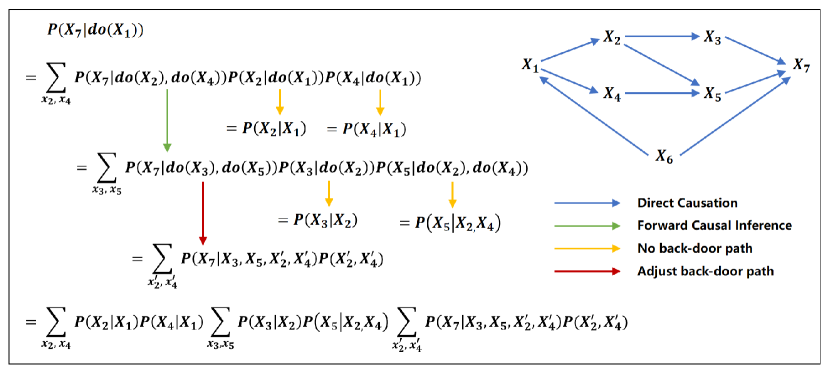
Figure 7: An example of Forward Counterfactual Inference algorithm. Here, $X_{i}$ is the same as $X_{i}^{\prime}$ to distinguish two recursions.

But on the contrary, the test process can be faster with Bayesian network in an SCM. Here, we provide an algorithm to realize forward counterfactual inference as shown in Algorithm 1, and provide an example to show the inference process as shown in Fig. 7.

The approaches to realize the codes in lines 1 and 3 in Algorithm 1 can be various, e.g., some variants of depth-first-search algorithm and breadth-first-search algorithm [89]. Thus, their time complexities are both $\mathcal{O}(|\mathbf{V}|+|\mathbf{E}|)$, if a Bayesian network $\mathcal{G}=(\mathbf{V},\mathbf{E})$ is given, where $\mathbf{V}$ is the node set and $\mathbf{E}$ is the edge set. Meanwhile, if the computational cost of factorization and adjustment are overlooked, the time complexity of the code in line 9 in Algorithm 1 is $\mathcal{O}(|\mathbf{V}|)$, because we only need to traverse all mediators in each pathway forward, and this process can be performed in parallel. Thus, the total time complexity of Algorithm 1 is $\mathcal{O}(|\mathbf{V}|^{2}+|\mathbf{V}||\mathbf{E}|)$. Thus, if the network structure of the Bayesian network is large, and it can be discovered accurately, the efficiency of SCM to infer counterfactuals would be better with polynomial time complexity.

Input: A Bayesian network $\mathcal{G}$ built on $\mathbf{V}=\{X_{1},\dots,X_{n}\}$ with one target $X_{i}$ and multiple sources $X_{j_{1}},\dots,X_{j_{p}}$.

Output: Distribution $P(X_{i}|do(X_{j_{1}}),\dots,do(X_{j_{p}}))$.

1

2Search one or multiple ordered causal pathways in $\mathcal{G}$ from the sources $X_{j_{1}},\dots,X_{j_{p}}$ to the target $X_{i}$;

3if $X_{j_{1}},\dots,X_{j_{p}}$ are all the direct causation for $X_{i}$ then

4       Search back-door paths (common causes) starting from $X_{j_{1}},\dots,X_{j_{p}}$ and $X_{i}$ reversely in $\mathcal{G}$.

5       if no back-door path within them then

6             return $P(X_{i}|X_{j_{1}},\dots,X_{j_{p}})$;

7      else

8             For every back-door path, select a group of direct predecessors, $\mathbf{W}\subset\mathbf{V}$, and then, according to back-door criterion (see Definition 2),

9             return $\sum_{w}P(X_{i}|X_{j_{1}},\dots,X_{j_{p}},W)P(W)$;

10      

11

12Otherwise, for $q$ pathways starting from $X_{j_{p}}$, select $q$ first mediators $X_{j_{p_{1}}},\dots,X_{j_{p_{q}}}$. Then, a group of source-mediator pairs, e.g., $(X_{j_{p}},X_{j_{p_{q}}})$, can be obtained;

13Factorize $P(X_{i}|do(X_{j_{1}}),\dots,do(X_{j_{p}}))$ as

$$P(X_{i}|do(X_{j_{1}}),\dots,do(X_{j_{p}}))$$ (11)

$$= \sum_{x_{j_{1_{1}}:j_{p_{q}}}}P(X_{i}|do(X_{j_{1_{1}}}),\dots,do(X_{j_{2_{1}}}),\dots,do(X_{j_{p_{q}}}))$$

$$\times\prod_{p}\prod_{q}P(X_{j_{p_{q}}}|do(X),X\in\mathbf{Pa}(X_{j_{p_{q}}})\subseteq\{X_{j_{1}:j_{p}}\}),$$

where $\mathbf{Pa}(X_{j_{p_{q}}})$ is the causal parents of $X_{j_{p_{q}}}$;

14Solve each distribution $P(\cdot|do(\cdot),\dots,do(\cdot))$ in Eq. (11) by Algorithm 1 recursively.

return $P(X_{i}|do(X_{j_{1}}),\dots,do(X_{j_{p}}))$.

Algorithm 1 Forward Counterfactual Inference

V Spatio-Temporal Graphical Counterfactuals

Back to the examples of counterfactual questions at the beginning of this article, that is, if a different investment strategy had been implemented, would we obtain higher returns? And, in computer networks, what changes would occur in network load if a node’s configuration had never been changed? And, would someone still purchase the product even if they had never been shown the advertisement? In these real-world scenarios, interactive behaviors with lagged causal effects are widely-existing. POM cannot answer these questions, because POM does not allow the interactive behaviors between experimental units (see SUTVA in Assumption 1), even with some temporal quasi-experimental approaches (e.g., Regression Discontinuity Design [90, 91] and Differences in Differences [92, 93]). And this is the same to SCM, because the foundational Bayesian network is a DAG that also does not allow mutual connections between network nodes. Thus, to answer these counterfactual queries for interactive units and lagged causal effects, a concept of spatio-temporal graphical counterfactuals is proposed here.

V-A Spatio-Temporal Bayesian Networks

Before the buildings of SCM, actually, various causal graphical models have been proposed to model the spatio-temporal causality. As shown in Fig. 8, Temporal Bayesian Network [64, 94] are proposed to model the momentary causal dependency in a first-order Markov process. Further, Dynamical Bayesian Networks [64] are proposed to represent a combination of multiple Temporal Bayesian Networks. Full Time Graph [25] is proposed to summarize the temporal Bayesian dependency at full timestamps. Note that, Full Time Graph allows the instantaneous causal effects between two units (or variables) in a high-order Markov process, but it only allows strictly stationary causality, that is, the causal dependencies do not change with time. Moreover, Full Time Graph is proved to uniquely decomposed into multiple high-order Temporal Bayesian Networks, named UCN, if the instantaneous causal effects is not allowed [95]. The comparisons of these causal graphs are shown in TABLE II.

Figure 8: Diagrams of various causal graphs.

TABLE II: Comparisons of various causal graphs.

	Temporal Bayesian Network	Dynamical Bayesian Networks	Full Time Graph	Spatio-Temporal Bayesian Networks
High-order causation	$\times$	$\times$	$\checkmark$	$\checkmark$
Instantaneous causation	$\times$	$\checkmark$	$\checkmark$	$\checkmark$
Nonstationary causation	$\times$	$\checkmark$	$\times$	$\checkmark$

Thus, based on the characteristics of these causal graphs, Spatio-Temporal Bayesian Networks (STBNs) are defined as a group of DAGs with different timestamps, as shown in Fig. 8. In STBNs, intuitively, the nodes are not equivalent to the variables, but represent the state of the variables at some time steps. With the assumptions of causal Markov (see Assumption 6) and faithfulness (see Assumption 7), the joint distribution of all nodes can be factorized as

$$P(X_{1,t},\dots,X_{n,t},X_{1,t-1},\dots,X_{n,t-T+1})$$ (12)

$$= \prod_{\tau=0}^{T-1}\prod_{i=1}^{n}P(X_{i,t-\tau}|\mathbf{Pa}(X_{i,t-\tau})),$$

where $X_{1},\dots,X_{n}$ are the variables, and the timestamps are in range of $0\sim T-1$. Theoretically, infinite time steps are allowed in STBNs, but it is usually finite in practice.

To guarantee the global and unique DAG in STBNs, a temporal assumption is introduced as

Assumption 9 (Temporal Assumption).

In STBNs, the cause node precedes or parallels the effect node in time.

This assumption does not allow the directed cause-effect pairs from now to the past, e.g., $X_{i,t-\tau_{1}}\rightarrow X_{j,t-\tau_{2}},\tau_{1}<\tau_{2}$. And this guarantees the functionally identifiable network structure without Markov equivalence class [25, 95, 96]. Moreover, the causal sufficiency assumption (see Assumption 8) is also needed to guarantee the unconfoundedness.

Then, if STBNs are given, the spatial-temporal counterfactuals can be inferred through Algorithm 1, because the global and local STBNs are both DAG. Compared with the naive Bayesian networks, STBNs have the spatio-temporal concept, and the inferring process is naturally forward along with time. This enables to define the momentary interventions for every time steps, and all the interventions would work sequentially, instead of at the same time, like in Algorithm 1. If fully consider this property, the inference algorithm can be faster.

V-B Nonstationarity of STBNs

Nonstationarity is a significant topic in researches on time series. Actually, however, the reasons inducing it are likely to be different from the view of causality. Three of the most currently popular reasons are:

1. Trending: The time series have ascending or descending trending for long terms.

2. Time-varying Variance: The variances of additive noise are time-varying, that is also called as heterogeneous causality in papers [97, 98].

3. Nonstationary Causality: The structures of STBNs change over time, and at least once, as shown in Fig. 9.

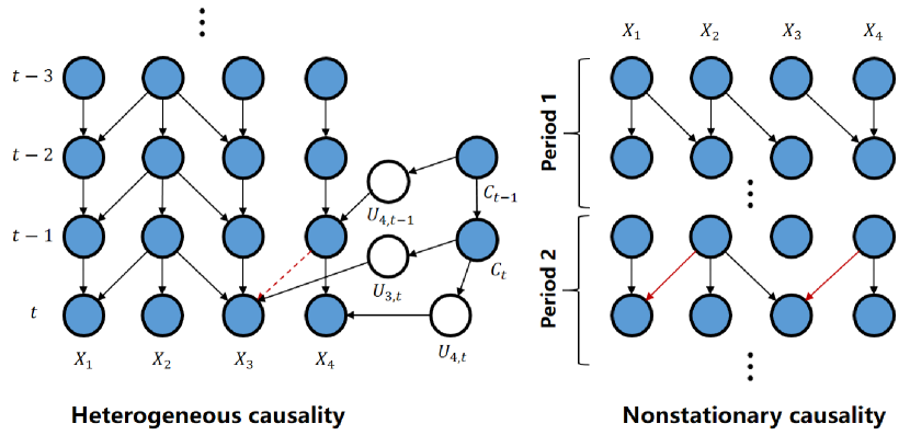
Figure 9: Diagrams of nonstationary causality and heterogeneous causality. Here, $C_{t-\tau}=t-\tau,\tau=0,\dots,T-1$ are usually assumed, thus, they are observable, instead of hidden variable.

For the trending time series, an effective approach is to calculate differences of time series in preprocessing. This approach enables to obtain the differential time series, that is the observations of system dynamics, like Eq. (13). This implied, the dynamics is stable during the period of time, and the structures of STBNs do not change, or in another word, the differential time series are stationary. Thus, if the dynamics equations, e.g., Eq. (13), are not equal to zero, the causal links in STBNs are identifiable through the Jacobian matrix of dynamics [99, 100, 101, 102].

For the case of time-varying variance, the causal identifiability is up to the mutually independent exogenous additive noises [96]. That is, if there is no causal connection between two additive noise nodes, the causation is identifiable. Thus, an effective approach is to relate the time-varying noises with a common timestamp, and the timestamps at all time steps are observable confounders $C_{t-\tau},\tau=0,\dots,T-1$ [103, 97, 104, 98]. As shown in Fig. 9, there are three causal pathways, that is, $C_{t-1}\rightarrow U_{4,t-1}\rightarrow X_{4,t-1}$, $C_{t-1}\rightarrow C_{t}\rightarrow U_{3,t}\rightarrow X_{3,t}$, and $C_{t-1}\rightarrow C_{t}\rightarrow U_{4,t}\rightarrow X_{4,t}$. Thus, if $C_{t}$ and $C_{t-1}$ are hidden, the spurious connection between $X_{4,t-1}$ and $X_{3,t}$ would be detected, like the dotted line in Fig. 9. However, $C_{t}$ and $C_{t-1}$ are usually known as the timestamp $t$ and $t-1$, thus, $C_{t}$ and $C_{t-1}$ block the fork paths between $X_{4,t-1},X_{3,t}$ and $X_{4,t}$. Then, the noise variables $U_{4,t-1},U_{3,t}$ and $U_{4,t}$ are mutually independent. Thus, it is causally identifiable. Note that, however, the premise to do so is that any hidden confounders in the case of time-varying variance can be written as smooth or non-smooth functions of timestamps [98].

Nonstationary causality is challenging but critical, especially for the case of frequently changing structures. To identify the nonstationary causality, one approach is to use sliding windows to identify causation within different time periods, as shown in Fig. 9. For each sliding window, it is assumed that the causal structure is invariant, and then, a group of samples would be input to identification algorithms, e.g., [105, 106, 107, 108, 95], to identify a invariant structure during this period. However, if the network changes are frequent, the samples used for identification during a short-term period would be few, but in contrast, we usually need sufficient samples to accept the significance of causal connections. Thus, another reasonable approach is to identify the change points first, and then, identify the causality with the corresponding periods [109, 110]. However, this still does not work in the extreme case of frequently changing, because the samples between two change points may be few. Moreover, there are some other approaches to view the nonstationary causality as a probabilistic normalized flow, and then use variational Bayesian inference to estimate it globally [111, 112, 113].

V-C STBNs and Complex networks

Here, we suppose STBNs model has been built, and it is associated with interactive time-series process of multivariate (or multiple units). Then, we further introduce complex network, another type of network model, to view the causal interactions in complex system. The network dynamics for variables $X_{i},\dots,X_{n}$ can be defined as

$$\frac{dX_{i,t}}{dt}=F(X_{i,t})+\sum_{j=1}^{n}A_{ij}G(X_{i,t},X_{j,t}),$$ (13)

where $F(\cdot)$ is the self-governed function of $X_{i}$, and $G(\cdot,\cdot)$ is the interactive function for node pairs $X_{i}$ and $X_{j}$. Moreover, $A_{ij}\geq 0$ is the connection between $X_{i}$ and $X_{j}$. Thus, if Eq. (13) is discretized, we can find it the same as first-order STBNs on stationary time series, as shown in Fig. 10.

Thus, the first-order STBNs have some good properties if network dynamics have. For example, if we want to know how to affect a node in STBNs by “intervening” another node, the practical inference steps may not be long, due to the small-world property [114, 115] or the scale-free property [116] of complex networks. Moreover, the counterfactual outcomes would not change because network systems have tolerance from external “interventions” [117, 118]. We would also know the synchronization [119, 120, 121, 122], controllability [123, 124, 125, 126, 127, 128, 129, 130], resilience [131, 132] of STBNs. We would also be able to sparsely identify the network structure even if the network size is large [6, 7], because the independence are equivalent to predictability in STBNs [95]. Also, the network size of STBNs can be reduced, because many complex networks can be simplified and still provide an insightful description of the causality of interest [133, 134]. This is meaningful to design counterfactual inference algorithm on smaller networks, and then obtain higher inference efficiency.

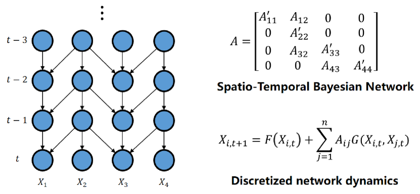
Figure 10: A diagram of discretized network dynamics. Here, $A$ is the adjacency matrix of the first-order STBNs, and $A_{ii}^{\prime},i=1,\dots,n$ represents the joined causal effect of $F$ and $G$.

VI Conclusion

In this work, we mainly focus on the spatio-temporal graphical counterfactuals, and organize an overview for it to discuss its theoretical foundations and application approaches. To discuss the theoretical foundations, a survey is investigated, and the definition of counterfactuals is defined based on the concept of potential outcome in the framework of POM firstly. And then, the framework of SCM is also introduced to infer counterfactuals through graphical languages, which are equivalent to the counterfactuals in POM. Further, to infer counterfactuals on intelligent machine autonomously, a Forward Counterfactual Inference algorithm is designed in this work, and it is able to recursively solve the counterfactual probability distribution, $P(X_{i}|do(X_{j_{1}}),\dots,do(X_{j_{p}}))$, with polynomial time complexity if multi-nodes interventions are conducted on $X_{j_{1}},\dots,X_{j_{p}}$. With this algorithm, the spatio-temporal graphical counterfactuals can be inferred if have two elements, that is, the network structure of STBNs and the corresponding algorithm to identify the network structure. This work not only discusses the identification algorithms in various nonstationary cases, but also discusses the feasibility to improve the algorithm efficiency from the view of complex networks.

References

- [1] O. Nelles, Nonlinear System Identification: From Classical Approaches to Neural Networks, Fuzzy Models, and Gaussian Processes (2nd edition). Springer, 2020.
- [2] S. L. Brunton, J. L. Proctor, and J. N. Kutz, “Discovering governing equations from data by sparse identification of nonlinear dynamical systems,” Proceedings of the National Academy of Sciences, vol. 113, no. 15, pp. 3932–3937, 2016.
- [3] W. Zhao, E. Weyer, and G. Yin, “A general framework for nonparametric identification of nonlinear stochastic systems,” IEEE Transactions on Automatic Control, vol. 66, no. 6, pp. 2449–2464, 2021.
- [4] K. Zisis, C. P. Bechlioulis, and G. A. Rovithakis, “Control-enabling adaptive nonlinear system identification,” IEEE Transactions on Automatic Control, vol. 67, no. 7, pp. 3715–3721, 2022.
- [5] X. Liu, D. Chen, W. Wei, X. Zhu, and W. Yu, “Interpretable sparse system identification: Beyond recent deep learning techniques on time-series prediction,” in International Conference on Learning Representations, 2024. [Online]. Available: https://openreview.net/forum?id=aFWUY3E7ws
- [6] T.-T. Gao and G. Yan, “Autonomous inference of complex network dynamics from incomplete and noisy data,” Nature Computational Science, vol. 2, no. 3, pp. 160–168, 2022.
- [7] B. Prasse and P. V. Mieghem, “Predicting network dynamics without requiring the knowledge of the interaction graph,” Proceedings of the National Academy of Sciences, vol. 119, no. 44, p. e2205517119, 2022.
- [8] C. M. Bishop, Pattern recognition and machine learning. Springer, 2006.
- [9] M. Kang, R. Zhu, D. Chen, C. Li, W. Gu, X. Qian, and W. Yu, “A cross-modal generative adversarial network for scenarios generation of renewable energy,” IEEE Transactions on Power Systems, vol. 39, no. 2, pp. 2630–2640, 2024.
- [10] D. P. Kingma and M. Welling, “Auto-encoding variational bayes,” arXiv preprint arXiv:1312.6114. [Online]. Available: https://arxiv.org/abs/1312.6114
- [11] I. Goodfellow, J. Pouget-Abadie, M. Mirza, B. Xu, D. Warde-Farley, S. Ozair, A. Courville, and Y. Bengio, “Generative adversarial nets,” Advances in Neural Information Processing Systems, vol. 27, 2014.
- [12] D. Rezende and S. Mohamed, “Variational inference with normalizing flows,” in International Conference on Machine Learning. PMLR, 2015, pp. 1530–1538.
- [13] J. Ho, A. Jain, and P. Abbeel, “Denoising diffusion probabilistic models,” in Advances in Neural Information Processing Systems, vol. 33. Curran Associates, Inc., 2020, pp. 6840–6851.
- [14] J. Song, C. Meng, and S. Ermon, “Denoising diffusion implicit models,” in International Conference on Learning Representations, 2021. [Online]. Available: https://openreview.net/forum?id=St1giarCHLP
- [15] Y. Song, J. Sohl-Dickstein, D. P. Kingma, A. Kumar, S. Ermon, and B. Poole, “Score-based generative modeling through stochastic differential equations,” in International Conference on Learning Representations, 2021. [Online]. Available: https://openreview.net/forum?id=PxTIG12RRHS
- [16] J. Pearl, Causality: Models, Reasoning, and Inference (2nd edition). Cambridge University Press, 2009.
- [17] G. W. Imbens and D. B. Rubin, Causal inference in statistics, social, and biomedical sciences. Cambridge University Press, 2015.
- [18] R. Ness, K. Paneri, and O. Vitek, “Integrating markov processes with structural causal modeling enables counterfactual inference in complex systems,” in Advances in Neural Information Processing Systems, vol. 32, 2019.
- [19] X. Chen, Z. Wang, H. Xu, J. Zhang, Y. Zhang, W. X. Zhao, and J.-R. Wen, “Data augmented sequential recommendation based on counterfactual thinking,” IEEE Transactions on Knowledge and Data Engineering, vol. 35, no. 9, pp. 9181–9194, 2023.
- [20] N. Seedat, F. Imrie, A. Bellot, Z. Qian, and M. van der Schaar, “Continuous-time modeling of counterfactual outcomes using neural controlled differential equations,” in International Conference on Machine Learning, vol. 162, 2022, pp. 19 497–19 521.
- [21] B. Bevilacqua, K. Nikiforou, B. Ibarz, I. Bica, M. Paganini, C. Blundell, J. Mitrovic, and P. Veličković, “Neural algorithmic reasoning with causal regularisation,” in International Conference on Machine Learning, vol. 202. PMLR, 2023, pp. 2272–2288.
- [22] K. He, L. Liu, Y. Zhang, Y. Wang, Q. Liu, and G. Wang, “Learning counterfactual explanation of graph neural networks via generative flow network,” IEEE Transactions on Artificial Intelligence, 2024. [Online]. Available: https://ieeexplore.ieee.org/abstract/document/10496445
- [23] K. Fujii, K. Takeuchi, A. Kuribayashi, N. Takeishi, Y. Kawahara, and K. Takeda, “Estimating counterfactual treatment outcomes over time in complex multiagent scenarios,” IEEE Transactions on Neural Networks and Learning Systems, 2024. [Online]. Available: https://ieeexplore.ieee.org/abstract/document/10445111
- [24] J. Pearl, M. Glymour, and N. P. Jewell, Causal inference in statistics: A primer. John Wiley & Sons, 2016.
- [25] J. Peters, D. Janzing, and B. Schölkopf, Elements of causal inference: foundations and learning algorithms. The MIT Press, 2017.
- [26] J. Pearl and D. Mackenzie, The book of why: the new science of cause and effect. Basic Books, 2018.
- [27] D. B. Rubin, “Causal inference using potential outcomes,” Journal of the American Statistical Association, vol. 100, no. 469, pp. 322–331, 2005.
- [28] R. P. Althauser and D. B. Rubin, “The computerized construction of a matched sample,” American Journal of Sociology, vol. 76, no. 2, pp. 325–346, 1970.
- [29] W. G. Cochran and D. B. Rubin, “Controlling bias in observational studies: A review,” Sankhyā: The Indian Journal of Statistics, Series A (1961-2002), vol. 35, no. 4, pp. 417–446, 1973.
- [30] D. B. Rubin, “Multivariate matching methods that are equal percent bias reducing, i: Some examples,” Biometrics, vol. 32, no. 1, pp. 109–120, 1976.
- [31] E. A. Stuart and D. B. Rubin, “Matching with multiple control groups with adjustment for group differences,” Journal of Educational and Behavioral Statistics, vol. 33, no. 3, pp. 279–306, 2008.
- [32] P. R. Rosenbaum and D. B. Rubin, “The central role of the propensity score in observational studies for causal effects,” Biometrika, vol. 70, no. 1, pp. 41–55, 1983.
- [33] D. B. Rubin and N. Thomas, “Matching using estimated propensity scores: Relating theory to practice,” Biometrics, vol. 52, no. 1, pp. 249–264, 1996.
- [34] D. B. Rubin, “Estimating causal effects from large data sets using propensity scores,” Annals of Internal Medicine, vol. 127, no. 8, pp. 757–763, 1997.
- [35] M. Caliendo and S. Kopeinig, “Some practical guidance for the implementation of propensity score matching,” Journal of Economic Surveys, vol. 22, no. 1, pp. 31–72, 2008.
- [36] K. Pearson, “Liii. on lines and planes of closest fit to systems of points in space,” The London, Edinburgh, and Dublin Philosophical Magazine and Journal of Science, vol. 2, no. 11, pp. 559–572, 1901.
- [37] D. R. Cox, “The regression analysis of binary sequences,” Journal of the Royal Statistical Society: Series B (Methodological), vol. 20, no. 2, pp. 215–232, 1958.
- [38] C. A. Sims, “Macroeconomics and reality,” Econometrica, vol. 48, no. 1, pp. 1–48, 1980.
- [39] O. J. Blanchard and D. Quah, “The dynamic effects of aggregate demand and supply disturbances,” pp. 655–673, 1988.
- [40] T. G. Kolda and B. W. Bader, “Tensor decompositions and applications,” SIAM Review, vol. 51, no. 3, pp. 455–500, 2009.
- [41] E. Acar, D. M. Dunlavy, T. G. Kolda, and M. Mørup, “Scalable tensor factorizations for incomplete data,” Chemometrics and Intelligent Laboratory Systems, vol. 106, no. 1, pp. 41–56, 2011.
- [42] C. C. Aggarwal et al., Recommender systems. Springer, 2016, vol. 1.
- [43] D. B. Rubin, “Randomization analysis of experimental data: The fisher randomization test comment,” Journal of the American Statistical Association, vol. 75, no. 371, pp. 591–593, 1980.
- [44] D. B. Rubin, “Inference and missing data,” Biometrika, vol. 63, no. 3, pp. 581–592, 1976.
- [45] D. B. Rubin, “Bayesian inference for causal effects: The role of randomization,” The Annals of Statistics, vol. 6, no. 1, pp. 34–58, 1978.
- [46] D. B. Rubin, “Estimating causal effects of treatments in randomized and nonrandomized studies.” Journal of Educational Psychology, vol. 66, no. 5, pp. 688–701, 1974.
- [47] J. Pearl, “Bayesian netwcrks: A model cf self-activated memory for evidential reasoning,” in Proceedings of the 7th Conference of the Cognitive Science Society, University of California, Irvine, CA, USA., 1985. [Online]. Available: https://ftp.cs.ucla.edu/pub/stat_ser/r43-1985.pdf
- [48] J. Pearl, “Fusion, propagation, and structuring in belief networks,” Artificial Intelligence, vol. 29, no. 3, pp. 241–288, 1986.
- [49] J. Pearl, “Evidential reasoning using stochastic simulation of causal models,” Artificial Intelligence, vol. 32, no. 2, pp. 245–257, 1987.
- [50] J. Pearl, Probabilistic reasoning in intelligent systems: networks of plausible inference. Morgan Kaufmann, 1988.
- [51] D. Geiger, T. Verma, and J. Pearl, “Identifying independence in bayesian networks,” Networks, vol. 20, no. 5, pp. 507–534, 1990.
- [52] J. Pearl, “[bayesian analysis in expert systems]: Comment: Graphical models, causality and intervention,” Statistical Science, vol. 8, no. 3, pp. 266–269, 1993.
- [53] J. Pearl, “Causal diagrams for empirical research,” Biometrika, vol. 82, no. 4, pp. 669–688, 1995.
- [54] J. Pearl, “Causal inference in statistics: An overview,” Statistics Surveys, vol. 3, pp. 96–146, 2009.
- [55] C. Glymour, K. Zhang, and P. Spirtes, “Review of causal discovery methods based on graphical models,” Frontiers in Genetics, vol. 10, p. 524, 2019.
- [56] B. Schölkopf, F. Locatello, S. Bauer, N. R. Ke, N. Kalchbrenner, A. Goyal, and Y. Bengio, “Toward causal representation learning,” Proceedings of the IEEE, vol. 109, no. 5, pp. 612–634, 2021.
- [57] M. J. Vowels, N. C. Camgoz, and R. Bowden, “D’ya like dags? a survey on structure learning and causal discovery,” ACM Computing Surveys, vol. 55, no. 4, pp. 1–36, 2022.
- [58] C. K. Assaad, E. Devijver, and E. Gaussier, “Survey and evaluation of causal discovery methods for time series,” Journal of Artificial Intelligence Research, vol. 73, pp. 767–819, 2022.
- [59] U. Hasan, E. Hossain, and M. O. Gani, “A survey on causal discovery methods for i.i.d. and time series data,” Transactions on Machine Learning Research, 2023. [Online]. Available: https://openreview.net/forum?id=YdMrdhGx9y
- [60] G. Lacerda, P. Spirtes, J. Ramsey, and P. O. Hoyer, “Discovering cyclic causal models by independent components analysis,” in Proceedings of the Twenty-Fourth Conference on Uncertainty in Artificial Intelligence (UAI), ser. UAI’08. AUAI Press, 2008, pp. 366–374.
- [61] P. Spirtes, “Directed cyclic graphical representations of feedback models,” in Proceedings of the Eleventh Annual Conference on Uncertainty in Artificial Intelligence (UAI), 1995, p. 491–498.
- [62] P. Forré and J. M. Mooij, “Markov properties for graphical models with cycles and latent variables,” arXiv preprint arXiv:1710.08775, 2017. [Online]. Available: https://arxiv.org/abs/1710.08775
- [63] S. Bongers, P. Forré, J. Peters, and J. M. Mooij, “Foundations of structural causal models with cycles and latent variables,” The Annals of Statistics, vol. 49, no. 5, pp. 2885 – 2915, 2021.
- [64] D. Koller and N. Friedman, Probabilistic graphical models: principles and techniques. MIT Press, 2009.
- [65] A. Barnard and D. Page, “Causal structure learning via temporal markov networks,” in Proceedings of the Ninth International Conference on Probabilistic Graphical Models, vol. 72. PMLR, 2018, pp. 13–24.
- [66] P. Spirtes, C. Meek, and T. Richardson, “Causal inference in the presence of latent variables and selection bias,” in Proceedings of the Eleventh Conference on Uncertainty in Artificial Intelligence (UAI). Morgan Kaufmann Publishers Inc., 1995, pp. 499–506.
- [67] P. Spirtes, “An anytime algorithm for causal inference,” in Proceedings of the Eighth International Workshop on Artificial Intelligence and Statistics, vol. R3. PMLR, 2001, pp. 278–285.
- [68] D. Colombo, M. H. Maathuis, M. Kalisch, and T. S. Richardson, “Learning high-dimensional directed acyclic graphs with latent and selection variables,” The Annals of Statistics, vol. 40, no. 1, pp. 294–321, 2012.
- [69] D. Colombo and M. H. Maathuis, “Order-independent constraint-based causal structure learning,” Journal of Machine Learning Research, vol. 15, no. 116, pp. 3921–3962, 2014.
- [70] J. M. Ogarrio, P. Spirtes, and J. Ramsey, “A hybrid causal search algorithm for latent variable models,” in Proceedings of the Eighth International Conference on Probabilistic Graphical Models, vol. 52. PMLR, 2016, pp. 368–379.
- [71] V. K. Raghu, J. D. Ramsey, A. Morris, D. V. Manatakis, P. Sprites, P. K. Chrysanthis, C. Glymour, and P. V. Benos, “Comparison of strategies for scalable causal discovery of latent variable models from mixed data,” International Journal of Data Science and Analytics, vol. 6, pp. 33–45, 2018.
- [72] M. Kocaoglu, A. Jaber, K. Shanmugam, and E. Bareinboim, “Characterization and learning of causal graphs with latent variables from soft interventions,” in Advances in Neural Information Processing Systems, vol. 32, 2019.
- [73] A. Jaber, M. Kocaoglu, K. Shanmugam, and E. Bareinboim, “Causal discovery from soft interventions with unknown targets: Characterization and learning,” in Advances in Neural Information Processing Systems, vol. 33, 2020, pp. 9551–9561.
- [74] A. Li, A. Jaber, and E. Bareinboim, “Causal discovery from observational and interventional data across multiple environments,” in Advances in Neural Information Processing Systems, vol. 36, 2023, pp. 16 942–16 956.
- [75] A. Rotnitzky and E. Smucler, “Efficient adjustment sets for population average causal treatment effect estimation in graphical models,” Journal of Machine Learning Research, vol. 21, no. 188, pp. 1–86, 2020.
- [76] J. Runge, “Necessary and sufficient graphical conditions for optimal adjustment sets in causal graphical models with hidden variables,” in Advances in Neural Information Processing Systems, vol. 34, 2021, pp. 15 762–15 773.
- [77] S. Triantafillou and G. Cooper, “Learning adjustment sets from observational and limited experimental data,” Proceedings of the AAAI Conference on Artificial Intelligence, vol. 35, no. 11, pp. 9940–9948, 2021.
- [78] E. Smucler, F. Sapienza, and A. Rotnitzky, “Efficient adjustment sets in causal graphical models with hidden variables,” Biometrika, vol. 109, no. 1, pp. 49–65, 2022.
- [79] G. W. Imbens and D. B. Rubin, “Bayesian inference for causal effects in randomized experiments with noncompliance,” The Annals of Statistics, vol. 25, no. 1, pp. 305–327, 1997.
- [80] F. Mealli and D. B. Rubin, “Assumptions allowing the estimation of direct causal effects,” Journal of Econometrics, vol. 112, no. 1, pp. 79–87, 2003.
- [81] D. B. Rubin, “Direct and indirect causal effects via potential outcomes,” Scandinavian Journal of Statistics, vol. 31, no. 2, pp. 161–170, 2004.
- [82] R. M. Baron and D. A. Kenny, “The moderator-mediator variable distinction in social psychological research: Conceptual, strategic, and statistical considerations,” Journal of Personality and Social Psychology, vol. 51, no. 6, pp. 1173–1182, 1986.
- [83] A. F. Hayes, Introduction to mediation, moderation, and conditional process analysis: A regression-based approach (3rd edition). Guilford Publications, 2022.
- [84] D. P. Mackinnon and J. H. Dwyer, “Estimating mediated effects in prevention studies,” Evaluation Review, vol. 17, no. 2, pp. 144–158, 1993.
- [85] D. P. MacKinnon, C. M. Lockwood, and J. Williams, “Confidence limits for the indirect effect: Distribution of the product and resampling methods,” Multivariate Behavioral Research, vol. 39, no. 1, pp. 99–128, 2004.
- [86] D. P. MacKinnon, A. J. Fairchild, and M. S. Fritz, “Mediation analysis,” Annual Review of Psychology, vol. 58, pp. 593–614, 2007.
- [87] M. E. Sobel, “Asymptotic confidence intervals for indirect effects in structural equation models,” Sociological Methodology, vol. 13, pp. 290–312, 1982.
- [88] M. E. Sobel, “Some new results on indirect effects and their standard errors in covariance structure models,” Sociological Methodology, vol. 16, pp. 159–186, 1986.
- [89] T. H. Cormen, C. E. Leiserson, R. L. Rivest, and C. Stein, Introduction to algorithms (4th edition). MIT press, 2022.
- [90] J. Hahn, P. Todd, and W. V. der Klaauw, “Identification and estimation of treatment effects with a regression-discontinuity design,” Econometrica, vol. 69, no. 1, pp. 201–209, 2001.
- [91] J. McCrary, “Manipulation of the running variable in the regression discontinuity design: A density test,” Journal of Econometrics, vol. 142, no. 2, pp. 698–714, 2008.
- [92] M. Bertrand, E. Duflo, and S. Mullainathan, “How much should we trust differences-in-differences estimates?” The Quarterly Journal of Economics, vol. 119, no. 1, pp. 249–275, 2004.
- [93] M. Lechner, “The estimation of causal effects by difference-in-difference methods,” Foundations and Trends in Econometrics, vol. 4, no. 3, pp. 165–224, 2011.
- [94] J. Sun, D. Taylor, and E. M. Bollt, “Causal network inference by optimal causation entropy,” SIAM Journal on Applied Dynamical Systems, vol. 14, no. 1, pp. 73–106, 2015.
- [95] M. Kang, D. Chen, N. Meng, G. Yan, and W. Yu, “Identifying unique causal network from nonstationary time series,” arXiv preprint arXiv:2211.10085, 2022. [Online]. Available: https://arxiv.org/abs/2211.10085
- [96] P. Hoyer, D. Janzing, J. M. Mooij, J. Peters, and B. Schölkopf, “Nonlinear causal discovery with additive noise models,” in Advances in Neural Information Processing Systems, vol. 21, 2008.
- [97] K. Zhang, B. Huang, J. Zhang, C. Glymour, and B. Schölkopf, “Causal discovery from nonstationary/heterogeneous data: Skeleton estimation and orientation determination,” in International Joint Conference on Artificial Intelligence, vol. 2017. NIH Public Access, 2017, pp. 1347–1353.
- [98] B. Huang, K. Zhang, J. Zhang, J. Ramsey, R. Sanchez-Romero, C. Glymour, and B. Schölkopf, “Causal discovery from heterogeneous/nonstationary data,” Journal of Machine Learning Research, vol. 21, no. 89, pp. 1–53, 2020.
- [99] B. Barzel and A.-L. Barabási, “Universality in network dynamics,” Nature Physics, vol. 9, no. 10, pp. 673–681, 2013.
- [100] P. Brouillard, S. Lachapelle, A. Lacoste, S. Lacoste-Julien, and A. Drouin, “Differentiable causal discovery from interventional data,” in Advances in Neural Information Processing Systems, vol. 33, 2020, pp. 21 865–21 877.
- [101] Y. He, P. Cui, Z. Shen, R. Xu, F. Liu, and Y. Jiang, “Daring: Differentiable causal discovery with residual independence,” in Proceedings of the 27th ACM SIGKDD Conference on Knowledge Discovery & Data Mining. Association for Computing Machinery, 2021, pp. 596–605.
- [102] A. Zhang, F. Liu, W. Ma, Z. Cai, X. Wang, and T.-S. Chua, “Boosting causal discovery via adaptive sample reweighting,” in International Conference on Learning Representations, 2023. [Online]. Available: https://openreview.net/forum?id=LNpMtk15AS4
- [103] B. Huang, K. Zhang, and B. Schölkopf, “Identification of time-dependent causal model: a gaussian process treatment,” in International Joint Conference on Artificial Intelligence, 2015, pp. 3561–3568.
- [104] B. Huang, K. Zhang, M. Gong, and C. Glymour, “Causal discovery and forecasting in nonstationary environments with state-space models,” in International Conference on Machine Learning, vol. 97. PMLR, 2019, pp. 2901–2910.
- [105] Y. He and Z. Geng, “Causal network learning from multiple interventions of unknown manipulated targets,” arXiv preprint arXiv:1610.08611, 2016. [Online]. Available: https://arxiv.org/abs/1610.08611
- [106] J. Peters, P. Bühlmann, and N. Meinshausen, “Causal inference by using invariant prediction: identification and confidence intervals,” Journal of the Royal Statistical Society. Series B (Statistical Methodology), vol. 78, no. 5, pp. 947–1012, 2016.
- [107] N. Pfister, P. Bühlmann, and J. Peters, “Invariant causal prediction for sequential data,” Journal of the American Statistical Association, vol. 114, no. 527, pp. 1264–1276, 2018.
- [108] R. Pamfil, N. Sriwattanaworachai, S. Desai, P. Pilgerstorfer, K. Georgatzis, P. Beaumont, and B. Aragam, “Dynotears: Structure learning from time-series data,” in Proceedings of the Twenty Third International Conference on Artificial Intelligence and Statistics, vol. 108. PMLR, 2020, pp. 1595–1605.
- [109] R. P. Adams and D. J. MacKay, “Bayesian online changepoint detection,” arXiv preprint arXiv:0710.3742, 2007. [Online]. Available: https://arxiv.org/abs/0710.3742
- [110] S. Aminikhanghahi and D. J. Cook, “A survey of methods for time series change point detection,” Knowledge and Information Systems, vol. 51, no. 2, pp. 339–367, 2017.
- [111] D. Rezende and S. Mohamed, “Variational inference with normalizing flows,” in International Conference on Machine Learning, vol. 37. PMLR, 2015, pp. 1530–1538.
- [112] G. Papamakarios, E. Nalisnick, D. J. Rezende, S. Mohamed, and B. Lakshminarayanan, “Normalizing flows for probabilistic modeling and inference,” Journal of Machine Learning Research, vol. 22, no. 57, pp. 1–64, 2021.
- [113] A. Javaloy, P. Sanchez-Martin, and I. Valera, “Causal normalizing flows: from theory to practice,” in Advances in Neural Information Processing Systems, vol. 36, 2023, pp. 58 833–58 864.
- [114] D. J. Watts and S. H. Strogatz, “Collective dynamics of ‘small-world’ networks,” Nature, vol. 393, no. 6684, pp. 440–442, 1998.
- [115] M. Newman and D. Watts, “Renormalization group analysis of the small-world network model,” Physics Letters A, vol. 263, no. 4, pp. 341–346, 1999.
- [116] A.-L. Barabási and R. Albert, “Emergence of scaling in random networks,” Science, vol. 286, no. 5439, pp. 509–512, 1999.
- [117] R. Albert, H. Jeong, and A.-L. Barabási, “Error and attack tolerance of complex networks,” Nature, vol. 406, no. 6794, pp. 378–382, 2000.
- [118] J. Gao, S. V. Buldyrev, S. Havlin, and H. E. Stanley, “Robustness of a network of networks,” Physical Review Letters, vol. 107, p. 195701, 2011.
- [119] S. Boccaletti, J. Kurths, G. Osipov, D. Valladares, and C. Zhou, “The synchronization of chaotic systems,” Physics Reports, vol. 366, no. 1, pp. 1–101, 2002.
- [120] A. Arenas, A. Díaz-Guilera, J. Kurths, Y. Moreno, and C. Zhou, “Synchronization in complex networks,” Physics Reports, vol. 469, no. 3, pp. 93–153, 2008.
- [121] S. Boccaletti, J. Almendral, S. Guan, I. Leyva, Z. Liu, I. Sendiña-Nadal, Z. Wang, and Y. Zou, “Explosive transitions in complex networks’ structure and dynamics: Percolation and synchronization,” Physics Reports, vol. 660, pp. 1–94, 2016.
- [122] D. Ghosh, M. Frasca, A. Rizzo, S. Majhi, S. Rakshit, K. Alfaro-Bittner, and S. Boccaletti, “The synchronized dynamics of time-varying networks,” Physics Reports, vol. 949, pp. 1–63, 2022.
- [123] X. F. Wang and G. Chen, “Pinning control of scale-free dynamical networks,” Physica A: Statistical Mechanics and its Applications, vol. 310, no. 3, pp. 521–531, 2002.
- [124] J. Lv and G. Chen, “A time-varying complex dynamical network model and its controlled synchronization criteria,” IEEE Transactions on Automatic Control, vol. 50, no. 6, pp. 841–846, 2005.
- [125] W. Yu, G. Chen, and J. Lv, “On pinning synchronization of complex dynamical networks,” Automatica, vol. 45, no. 2, pp. 429–435, 2009.
- [126] W. Yu, P. DeLellis, G. Chen, M. di Bernardo, and J. Kurths, “Distributed adaptive control of synchronization in complex networks,” IEEE Transactions on Automatic Control, vol. 57, no. 8, pp. 2153–2158, 2012.
- [127] W. Yu, G. Chen, J. Lv, and J. Kurths, “Synchronization via pinning control on general complex networks,” SIAM Journal on Control and Optimization, vol. 51, no. 2, pp. 1395–1416, 2013.
- [128] W. Yu, W. Ren, W. X. Zheng, G. Chen, and J. Lv, “Distributed control gains design for consensus in multi-agent systems with second-order nonlinear dynamics,” Automatica, vol. 49, no. 7, pp. 2107–2115, 2013.
- [129] Y.-Y. Liu, J.-J. Slotine, and A.-L. Barabási, “Controllability of complex networks,” Nature, vol. 473, no. 7346, pp. 167–173, 2011.
- [130] A. Li, S. P. Cornelius, Y.-Y. Liu, L. Wang, and A.-L. Barabási, “The fundamental advantages of temporal networks,” Science, vol. 358, no. 6366, pp. 1042–1046, 2017.
- [131] J. Gao, B. Barzel, and A.-L. Barabási, “Universal resilience patterns in complex networks,” Nature, vol. 530, no. 7590, pp. 307–312, 2016.
- [132] X. Liu, D. Li, M. Ma, B. K. Szymanski, H. E. Stanley, and J. Gao, “Network resilience,” Physics Reports, vol. 971, pp. 1–108, 2022.
- [133] J. Gao, “Intrinsic simplicity of complex systems,” Nature Physics, vol. 20, pp. 184–185, 2024.
- [134] V. Thibeault, A. Allard, and P. Desrosiers, “The low-rank hypothesis of complex systems,” Nature Physics, vol. 20, pp. 294–302, 2024.