tPARAFAC2: Tracking evolving patterns in (incomplete) temporal data

Abstract

Tensor factorizations have been widely used for the task of uncovering patterns in various domains. Often, the input is time-evolving, shifting the goal to tracking the evolution of underlying patterns instead. To adapt to this more complex setting, existing methods incorporate temporal regularization but they either have overly constrained structural requirements or lack uniqueness which is crucial for interpretation. In this paper, in order to capture the underlying evolving patterns, we introduce t(emporal)PARAFAC2 which utilizes temporal smoothness regularization on the evolving factors. We propose an algorithmic framework that employs Alternating Optimization (AO) and the Alternating Direction Method of Multipliers (ADMM) to fit the model. Furthermore, we extend the algorithmic framework to the case of partially observed data. Our numerical experiments on both simulated and real datasets demonstrate the effectiveness of the temporal smoothness regularization, in particular, in the case of data with missing entries. We also provide an extensive comparison of different approaches for handling missing data within the proposed framework.

1 Introduction

Temporal datasets capture the evolution of an event or a system as a sequence of time-stamped observations. Investigating such temporal datasets, uncovering latent patterns and the evolution of those patterns over time is crucial across various domains since it can provide insights into the underlying dynamic processes. For example, in neuroscience, capturing spatial networks of brain connectivity as well as their evolution over time holds the promise to improve our understanding of brain function [1]. Other examples are social network analysis, where evolving patterns may reveal changes in communities of users, or dynamic topic modeling which aims to detect the temporal evolution of topics, for instance, within a large collection of documents [2].

Temporal data frequently takes the form of a multidimensional array (i.e., a tensor) and the use of tensor factorizations has shown to be an effective tool for their analysis. The rationale of these unsupervised methods is to decompose the input into smaller but interpretable factors that reflect the main trends present. For example, Bader et al. [3] applied the CANDECOMP/PARAFAC (CP) decomposition [4, 5] on Enron email data (arranged as a third-order tensor with modes: authors, words, and time) and extracted interpretable factors directly connected to the company’s collapse. In [6], incorporating non-negativity allowed CP to improve prediction accuracy on missing entries on QoS (Quality-of-Service) data relevant to online services. However, these methods do not involve the intrinsic properties of the temporal dimension of the input. Thus, extensions of CP tailored for temporal data have been proposed [7, 8, 9]. Yu et al. [7] enhanced the CP decomposition with autoregressive regularization on both temporal and spatial dimensions, which allowed for more accurate forecasting. Time-aware Tensor Decomposition (TATD) [8] assumes smooth changes across data of consecutive time-points and simultaneously imposes sparsity regularization with strength that varies over time. SeekAndDestroy [9] updates a CP decomposition in an online fashion as new data is received, and keeps track of disappearing and emerging concepts. In all of these methods, nonetheless, the concepts uncovered by the factors must adhere to the CP structure, which means they are only allowed to change by a scalar multiplicator over time. This is a limitation when the task at hand is to discover evolving patterns.

In terms of capturing time-evolving patterns, other proposed methods in the literature follow the less structurally constrained Collective Matrix Factorization (CMF) paradigm [10], while incorporating additional temporal regularization [11, 12, 13, 14]. Yu et al. [11] proposed Temporal Matrix Factorization (TMF), which factorizes the input using a set of time-index dependent factors. The method proposed by Appel et al. [12] receives additional contextual inputs and factorizes the input assuming smooth changes over time. Under the same assumption of small changes across consecutive time-points, Hooi et al. proposed SMF (Seasonal Matrix Factorization) [13], an online method that involves updating the factors through small gradient descent steps to facilitate smooth factor evolution while also addressing the seasonality of uncovered patterns. This work has later been extended to accept multiple seasonal ‘regimes’ [14]. While CMF-based approaches provide more expressive factors that reflect the underlying evolving patterns in greater detail, they generally do not possess uniqueness guarantees for their solutions, which are necessary for interpretation [15].

In the middle ground between CP and CMF-based approaches lies the PARAFAC2 factorization [16], a technique that has shown its versatility and effectiveness across various fields such as in chemometrics in terms of analyzing measurements of samples with unaligned profiles [17], in neuroscience by allowing for subject-specific temporal profiles [18] and task-specific spatial maps [19], and in electronic health record (EHR) data analysis allowing for unaligned time profiles [20]. Apart from having uniqueness properties under certain conditions [21], PARAFAC2 offers the flexibility of allowing the factors to vary along one specific mode (evolving mode) in all these applications. Several adaptations of PARAFAC2 for temporal data have been proposed, each incorporating different temporal regularization techniques [22, 23, 24, 25, 26]. LogPar [22] regularizes the factor matrix in the time mode by assuming that columns of the factor matrix slowly change, and uses an exponential decay-based weight. COPA [23] and REPAIR [24] utilize M-spline-based temporal smoothness on the factor matrix extracted from the time mode. ATOM [25] ensures the smoothness of the components in the time mode by penalizing the difference between temporally consecutive factors. TedPar [26] is a PARAFAC2-based framework for EHR data that utilizes temporal smoothness to monitor smooth phenotypic changes. However, these studies focus on the regularization of the factors extracted from the time mode assuming static factors in other modes.

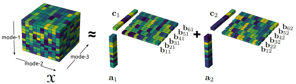
In this paper, we use the PARAFAC2 model to extract evolving patterns in time (as in Figure 1, where mode 3 is time and the evolving mode (mode 2) may correspond to, e.g., voxels to capture evolving spatial maps, words to capture evolving topics) and consider temporal regularization of such time-evolving patterns. In other words, we force the structure of the patterns to change smoothly over time and not their strength. Our contributions can be summarized as follows:

• We introduce the t(emporal)PARAFAC2 model and an AO-ADMM based algorithmic approach to fit the model,

• We consider two different ways of handling missing data, i.e., an Expectation Maximization (EM)-based approach and one employing Row-Wise (RW) updates, when fitting a regularized PARAFAC2 (and hence also tPARAFAC2) model using the AO-ADMM framework,

• Using extensive numerical experiments on synthetic data with slowly changing patterns with varying levels of noise and amounts of missing data, we demonstrate the effectiveness of tPARAFAC2 in terms of recovering the underlying patterns accurately,

• We demonstrate that while the EM-based approach and the RW updates are equally accurate, the EM-based approach is computationally more efficient,

• We use the proposed methods on two real data sets. In a chemometrics application, we demonstrate the added value of constraints on the evolving mode when fitting a PARAFAC2 model in the presence of missing data. In a metabolomics application, we use PARAFAC2 to capture evolving metabolite patterns from a dynamic metabolomics data set, and show the effectiveness of tPARAFAC2 in the case of high amounts of missing data.

This paper is an extension of our preliminary study [27] where we introduced t(emporal)PARAFAC2 and demonstrated its promise in noisy and low-signal settings, while also showing its limitation when the data does not follow the PARAFAC2 structure. Here, we extend the model and the algorithmic approach to incomplete data by considering two different algorithmic approaches to handle missing data. In addition to noisy settings, we also demonstrate the effectiveness of tPARAFAC2 in the case of missing data. We also utilize the proposed approaches in two real applications.

The rest of the paper is organized as follows: Subsection 1.1 describes the notation used in this work, section 2 introduces the PARAFAC2 factorization and relevant computational schemes, sections 3.1 and 3.2 introduce tPARAFAC2 and the AO-ADMM approach to compute the model, section 3.3 focuses on our proposed approaches for incorporating missing data and places them in the state-of-the-art while section 4 contains our experimental results.

1.1 Notation

In this paper, we adopt the tensor notation of [28]. The order of a tensor indicates the number of modes; in other words, the number of indices needed to specify each entry. In this regard, a vector is a tensor of order one and a matrix as a tensor of order two. Tensors with order of at least three are referred to as higher-order tensors. We use bold lowercase letters to denote vectors (e.g. ${\bm{\mathbf{{x}}}}$, ${\bm{\mathbf{{y}}}}$) and bold capital letters for matrices (e.g. ${\bm{\mathbf{{X}}}}$, ${\bm{\mathbf{{Y}}}}$). For higher-order tensors, we use bold uppercase Euler script letters (e.g. $\bm{\mathscr{{X}}}$, $\bm{\mathscr{{Y}}}$). Table 1 shows our notation for various tensor-related mathematical operations.

It is useful in practice to use slicing and refer to specific segments of a tensor. The higher-order equivalent of matrix rows and columns is referred to as fibers. We can obtain mode-$n$ fibers of a tensor by fixing the indices on all modes except the $n$-th. In the same manner, we can obtain (matrix) slices of a tensor by fixing all indices except two. To exemplify these concepts, consider a third-order tensor $\bm{\mathscr{{X}}}\in{\mathbb{R}}^{I\times J\times K}$: We can obtain any mode-$1$ fiber of $\bm{\mathscr{{X}}}$ by fixing $j$ and $k$ in $\bm{\mathscr{{X}}}{(:,j,k)}$ and any “frontal” slice by fixing $k$ in $\bm{\mathscr{{X}}}{(:,:,k)}$. Specifically for frontal slices, we are going to use the notation ${\bm{\mathbf{{X}}}}_{k}$.

Symbol	Operation
$\circ$	Outer product
$\otimes$	Kronecker product
$\odot$	Khatri-Rao product
$\ast$	Hadamard product
${\bm{\mathbf{{X}}}}^{{\sf T}}$	Matrix transpose
${\bm{\mathbf{{X}}}}^{-1}$	Matrix inverse
$\left\lVert\,\cdot\,\right\rVert_{F}$	Frobenius norm
$diag({\bm{\mathbf{{A}}}})$	diag operation

Table 1: Notation used for relevant mathematical operations.

2 Background

2.1 The PARAFAC2 factorization

Originally proposed by Harshman [16], PARAFAC2 models each frontal slice of a third order tensor $\bm{\mathscr{{X}}}\in{\mathbb{R}}^{I\times J\times K}$ as a product of three factors:

$$\begin{split}{\bm{\mathbf{{X}}}}_{k}\approx{\bm{\mathbf{{A}}}}{\bm{\mathbf{{D}}}}_{k}{\bm{\mathbf{{B}}}}_{k}^{{\sf T}}\\ {\{{\bm{\mathbf{{B}}}}_{k}}\}_{k=1}^{K}\in\mathscr{P}\end{split}$$ (1)

where ${\bm{\mathbf{{A}}}}\in{\mathbb{R}}^{I\times R}$, ${\bm{\mathbf{{D}}}}_{k}\in{\mathbb{R}}^{R\times R}$ is a diagonal matrix and ${\bm{\mathbf{{B}}}}_{k}\in{\mathbb{R}}^{J\times R}\;\forall\;k=1,\dots,K$. $R$ denotes the number of components. It is convenient to concatenate the diagonals of the $\{{\bm{\mathbf{{D}}}}_{k}\}_{k=1}^{K}$ as rows in a single factor matrix ${\bm{\mathbf{{C}}}}\in{\mathbb{R}}^{K\times R}$. The second line of Equation (1) denotes the constant cross-product constraint of PARAFAC2:

$$\mathscr{P}=\left\{\{{\bm{\mathbf{{B}}}}_{k}\}_{k=1}^{K}\mid{\bm{\mathbf{{B}}}}^{{\sf T}}_{k_{1}}{\bm{\mathbf{{B}}}}_{k_{1}}={\bm{\mathbf{{B}}}}^{{\sf T}}_{k_{2}}{\bm{\mathbf{{B}}}}_{k_{2}}\;\forall k_{1},\!k_{2}\in\{1,2,...,K\}\right\}.$$ (2)

We refer to this constraint as the PARAFAC2 constraint. Note that this formulation remains valid even if the frontal slices ${\bm{\mathbf{{X}}}}_{k}$ have different number of columns.

PARAFAC2 is considered to have an “essentially” unique solution up to permutation and scaling (under certain conditions) [21]. To understand these ambiguities, consider the formulation of PARAFAC2 for a specific slice as follows:

$${\bm{\mathbf{{X}}}}_{k}\approx\sum_{r=1}^{R}{\bm{\mathbf{{d}}}}_{kr}({\bm{\mathbf{{a}}}}_{r}\circ{\bm{\mathbf{{b}}}}_{kr})$$ (3)

where ${\bm{\mathbf{{d}}}}_{kr}={\bm{\mathbf{{D}}}}_{k}(r,r)$, ${\bm{\mathbf{{a}}}}_{r}={\bm{\mathbf{{A}}}}{(:,r)}$ and ${\bm{\mathbf{{b}}}}_{kr}={\bm{\mathbf{{B}}}}_{k}(:,r)$. Reordering the components of the summation does not impact the quality of the solution, constituting a permutation ambiguity. Moreover, if any of ${\bm{\mathbf{{d}}}}_{kr}$, ${\bm{\mathbf{{a}}}}_{r}$ and ${\bm{\mathbf{{b}}}}_{kr}$ is scaled by $\gamma$ and the other two are scaled simultaneously by factors with product $\frac{1}{\gamma}$ (the PARAFAC2 constraint should be satisfied at all times), the model estimate of the slice is consistent and the solution is considered equivalent (scaling ambiguity). The case of $\gamma=-1$ corresponds to the sign ambiguity. While such ambiguities do not interfere with the interpretation of the captured factors, there is an additional challenge due to the sign ambiguity in PARAFAC2 since ${\bm{\mathbf{{d}}}}_{kr}$ can arbitrarily flip signs together with ${\bm{\mathbf{{b}}}}_{kr}$ [16]. One possible solution to fix the sign ambiguity is to impose non-negativity constraints on ${\bm{\mathbf{{C}}}}$ [16, 21].

Figure 1: Illustration of a 2-component PARAFAC2 model of a third-order tensor, where mode 2 (with ${\bm{\mathbf{{b}}}}_{kr}$, for $k=1,...,6$ and $r=1,2$) is the evolving mode.

2.2 Algorithms for fitting PARAFAC2

2.2.1 Alternating Least Squares (ALS)

Much work in the literature has focused on finding an efficient algorithm for fitting the PARAFAC2 model. Kiers et al. [21] proposed the ‘direct fitting’ method, which parametrized each ${\bm{\mathbf{{B}}}}_{k}$ as ${\bm{\mathbf{{B}}}}_{k}={\bm{\mathbf{{P}}}}_{k}{\bm{\mathbf{{B}}}}$, where each ${\bm{\mathbf{{P}}}}_{k}$ is constrained to have orthonormal columns. Fitting the PARAFAC2 model is then formulated as the following optimization problem:

$$\begin{split}\min_{{\bm{\mathbf{{A}}}},\{{\bm{\mathbf{{P}}}}_{k}\}_{k=1}^{K},{\bm{\mathbf{{B}}}},{\bm{\mathbf{{C}}}}}&\quad\left\{\sum_{k=1}^{K}\left\lVert\,{\bm{\mathbf{{X}}}}_{k}\!-\!{\bm{\mathbf{{A}}}}{\bm{\mathbf{{D}}}}_{k}({\bm{\mathbf{{P}}}}_{k}{\bm{\mathbf{{B}}}})^{{\sf T}}\,\right\rVert_{F}^{2}\right\}\\ \text{subject to}\quad&\quad{\bm{\mathbf{{P}}}}_{k}^{{\sf T}}{\bm{\mathbf{{P}}}}_{k}={\bm{\mathbf{{I}}}}\quad\forall\;k=1,\dots,K.\end{split}$$ (4)

This parametrization encapsulates the PARAFAC2 constraint as ${\bm{\mathbf{{B}}}}_{k}^{{\sf T}}{\bm{\mathbf{{B}}}}_{k}={\bm{\mathbf{{B}}}}^{{\sf T}}{\bm{\mathbf{{P}}}}_{k}^{{\sf T}}{\bm{\mathbf{{P}}}}_{k}{\bm{\mathbf{{B}}}}={\bm{\mathbf{{B}}}}^{{\sf T}}{\bm{\mathbf{{B}}}}$, which is constant across all values of $k$. Fixing all factors except $\{{\bm{\mathbf{{P}}}}_{k}\}_{k=1}^{K}$ results in orthogonal Procrustes problems and SVD is used to solve them. Then each frontal slice is multiplied by ${\bm{\mathbf{{P}}}}_{k}$ and problem (4) is minimized with respect to ${\bm{\mathbf{{A}}}}$, ${\bm{\mathbf{{B}}}}$ and ${\bm{\mathbf{{C}}}}$ by alternatingly solving the respective least squares problems until convergence. This approach is referred to as the PARAFAC2 ALS algorithm.

Imposing additional constraints is often beneficial, for example, to enhance interpretability, incorporate domain knowledge, or improve robustness to noise. While it is possible to impose certain constraints on factor matrices ${\bm{\mathbf{{A}}}}$ and ${\bm{\mathbf{{C}}}}$ using an ALS-based algorithm when solving problem (4), it is difficult to do so for $\{{\bm{\mathbf{{B}}}}_{k}\}_{k=1}^{K}$ factor matrices. Recently, the ‘flexible coupling’ approach, which formulates the PARAFAC2 constraint as an additional penalty term, was introduced to incorporate non-negativity constraints in all modes [29]. In theory, some other constraints could also be incorporated by employing specialized constrained least-squares solvers. However, as described in [29], the method suffers from time-consuming tuning of the penalty parameter.

2.2.2 Alternating Optimization - Alternating Direction Method of Multipliers (AO-ADMM)

A more flexible algorithmic approach for fitting the PARAFAC2 model is the AO-ADMM-based algorithmic approach, which facilitates the use of a variety of constraints on all modes [30]. The AO-ADMM-based approach formulates the regularized PARAFAC2 problem as:

$$\begin{split}\min_{{\bm{\mathbf{{A}}}},\{{\bm{\mathbf{{B}}}}_{k}\}_{k=1}^{K},{\bm{\mathbf{{C}}}}}\quad&\Bigg{\{}\sum_{k=1}^{K}\left\lVert\,{\bm{\mathbf{{X}}}}_{k}\!-\!{\bm{\mathbf{{A}}}}{\bm{\mathbf{{D}}}}_{k}{\bm{\mathbf{{B}}}}_{k}^{T}\,\right\rVert_{F}^{2}+g_{{\bm{\mathbf{{A}}}}}({\bm{\mathbf{{A}}}})\\ &\quad+g_{{\bm{\mathbf{{B}}}}}(\{{\bm{\mathbf{{B}}}}_{k}\}_{k=1}^{K})+g_{{\bm{\mathbf{{D}}}}}(\{{\bm{\mathbf{{D}}}}_{k}\}_{k=1}^{K})\Bigg{\}}\\ \text{subject to}\quad\quad&\quad\{{\bm{\mathbf{{B}}}}_{k}\}_{k=1}^{K}\in\mathscr{P}\quad\forall\;k=1,\dots,K\end{split}$$ (5)

where $g_{{\bm{\mathbf{{A}}}}}$, $g_{{\bm{\mathbf{{B}}}}}$ and $g_{{\bm{\mathbf{{D}}}}}$ denote regularization penalties imposed on respective factors. In principle, after the augmented Lagrangian is formed, the algorithm alternates between solving the subproblems for each of the factor matrices using ADMM. To solve the non-convex subproblems of the evolving factors $\{{\bm{\mathbf{{B}}}}_{k}\}_{k=1}^{K}$, an effective iterative scheme is proposed to project the evolving factors onto $\mathscr{P}$ [30]. This procedure is repeated until changes in the solution are sufficiently small, which is indicated by small relative or absolute change in the objective function of Equation (5), and as long as the constraints are satisfied adequately (i.e. small ‘feasibility’ gaps):

$$\lVert f^{(n+1)}-f^{(n)}\rVert<\epsilon_{abs}\ \ \textit{OR}\ \ \frac{\lVert f^{(n+1)}-f^{(n)}\rVert}{\lVert f^{(n)}\rVert}<\epsilon_{rel}$$

$$\textit{AND}\ \frac{\left\lVert\,{\bm{\mathbf{{M}}}}-{\bm{\mathbf{{Z}}}}_{{\bm{\mathbf{{M}}}}}\,\right\rVert}{\left\lVert\,{\bm{\mathbf{{M}}}}\,\right\rVert} <\epsilon_{feasibility}$$

where $f^{(n+1)}$ and $f^{(n)}$ denote the function value at iteration $n+1$ and $n$, respectively, and for each factor matrix ${\bm{\mathbf{{M}}}}$, ${\bm{\mathbf{{Z}}}}_{{\bm{\mathbf{{M}}}}}$ denotes the respective auxiliary variable. The last condition should hold for all factor matrices that involve regularization. The tolerances $\epsilon_{abs}$, $\epsilon_{rel}$ and $\epsilon_{feasibility}$ are user-defined. More information about the exit conditions can be found in the Supplementary material.

3 Proposed methodology

3.1 tPARAFAC2

When PARAFAC2 is used to analyze time-evolving data with frontal slices ${\bm{\mathbf{{X}}}}_{k}$ changing in time, $k=1,...,K$, $\{{\bm{\mathbf{{B}}}}_{k}\}_{k=1}^{K}$ factor matrices can capture the structural changes of the patterns in time while $\{{\bm{\mathbf{{D}}}}_{k}\}_{k=1}^{K}$ capture the strength over time. Combining information from both sets of factors allows for a thorough understanding of the underlying evolving patterns. For example, this key property of PARAFAC2 has been previously used to uncover evolving spatial brain activation maps (i.e., spatial dynamics) from fMRI data [31, 1].

However, without additional constraints, PARAFAC2 is not time-aware, i.e., the model is unable to take into account the sequential nature of the temporal dimension. One can confirm this by applying the factorization on two reordered versions of a dataset: the factorizations will be respectively reordered. While mathematically acceptable, the two versions could potentially describe two different unfoldings of events.

To tackle this problem, we introduce t(emporal)PARAFAC2, which is formulated as [27]:

$$\begin{split}\min_{{\bm{\mathbf{{A}}}},\{{\bm{\mathbf{{B}}}}_{k}\}_{k=1}^{K},{\bm{\mathbf{{C}}}}}\quad&\Bigg{\{}\sum_{k=1}^{K}\left\lVert\,{\bm{\mathbf{{X}}}}_{k}\!-\!{\bm{\mathbf{{A}}}}{\bm{\mathbf{{D}}}}_{k}{\bm{\mathbf{{B}}}}_{k}^{T}\,\right\rVert_{F}^{2}+g_{{\bm{\mathbf{{A}}}}}({\bm{\mathbf{{A}}}})\\ &\quad+\lambda_{B}\sum_{k=2}^{K}\left\lVert\,{\bm{\mathbf{{B}}}}_{k}\!-\!{\bm{\mathbf{{B}}}}_{k-1}\,\right\rVert_{F}^{2}+g_{{\bm{\mathbf{{D}}}}}(\{{\bm{\mathbf{{D}}}}_{k}\}_{k=1}^{K})\Bigg{\}}\\ \text{subject to}\quad\quad&\quad\{{\bm{\mathbf{{B}}}}_{k}\}_{k=1}^{K}\in\mathscr{P}\quad\forall\;k=1,\dots,K\ .\end{split}$$ (6)

Equation (6) is essentially the regularized PARAFAC2 AO-ADMM problem (Equation (5)) with

$$g_{{\bm{\mathbf{{B}}}}}(\{{\bm{\mathbf{{B}}}}_{k}\}_{k=1}^{K})=\lambda_{B}\sum_{k=2}^{K}\left\lVert\,{\bm{\mathbf{{B}}}}_{k}\!-\!{\bm{\mathbf{{B}}}}_{k-1}\,\right\rVert_{F}^{2}.\vspace{-0.1cm}$$ (7)

This formulation assumes that the data exhibits fine temporal granularity or that the underlying patterns evolve slowly over time - similar to the temporal regularization previously used in CMF [12]. Therefore, tPARAFAC2 regularizes ${\bm{\mathbf{{B}}}}_{k}$ factor matrices that correspond to consecutive time slices to be similar, with the regularization strength controlled by $\lambda_{\bm{\mathbf{{B}}}}$. Due to the scaling ambiguity, it is crucial to have norm-based regularization in the other modes [30]. Furthermore, to overcome the sign ambiguity of PARAFAC2, we impose non-negativity on the factors of the third mode. Therefore, in Problem (6) we set

$$g_{{\bm{\mathbf{{A}}}}}({\bm{\mathbf{{A}}}}) =\lambda_{A}\left\lVert\,{\bm{\mathbf{{A}}}}\,\right\rVert_{F}^{2}$$

$$g_{{\bm{\mathbf{{D}}}}}(\{{\bm{\mathbf{{D}}}}_{k}\}_{k=1}^{K}) =\sum_{k=1}^{K}\bigl{(}\lambda_{{\bm{\mathbf{{D}}}}}\left\lVert\,{\bm{\mathbf{{D}}}}_{k}\,\right\rVert_{F}^{2}+\iota_{\mathbb{R}_{+}}({\bm{\mathbf{{D}}}}_{k})\bigr{)}\vspace{-0.3cm}$$

where hyperparameters $\lambda_{A}$ and $\lambda_{D}$ control the strength of the ridge penalties and $\iota_{\mathbb{R}_{+}}({\bm{\mathbf{{D}}}}_{k})$ is the indicator function for the non-negative orthant.

3.2 Optimization

We solve Problem (6) using the PARAFAC2 AO-ADMM framework [30]. The augmented Lagrangian of the full optimization problem is given by:

$$\mathcal{L}=\sum_{k=1}^{K}\lVert{\bm{\mathbf{{X}}}}_{k}-{\bm{\mathbf{{A}}}}{\bm{\mathbf{{D}}}}_{k}{\bm{\mathbf{{B}}}}_{k}^{{\sf T}}\rVert^{2}_{F}+\lambda_{{\bm{\mathbf{{A}}}}}\lVert{\bm{\mathbf{{A}}}}\rVert^{2}_{F}+\lambda_{{\bm{\mathbf{{D}}}}}\sum_{k=1}^{K}\lVert{\bm{\mathbf{{D}}}}_{k}\rVert^{2}_{F}$$

$$+\lambda_{B}\sum_{k=2}^{K}\lVert{\bm{\mathbf{{Z}}}}_{{\bm{\mathbf{{B}}}}_{k}}-{\bm{\mathbf{{Z}}}}_{{\bm{\mathbf{{B}}}}_{k-1}}\rVert^{2}_{F}+\sum_{k=1}^{K}\frac{\rho_{{\bm{\mathbf{{B}}}}_{k}}}{2}\lVert{\bm{\mathbf{{B}}}}_{k}-{\bm{\mathbf{{Z}}}}_{{\bm{\mathbf{{B}}}}_{k}}+{\bm{\mathbf{{\mu}}}}_{{\bm{\mathbf{{Z}}}}_{{\bm{\mathbf{{B}}}}_{k}}}\rVert^{2}_{F}$$

$$+\iota_{\mathscr{P}}(\{{\bm{\mathbf{{Y}}}}_{{\bm{\mathbf{{B}}}}_{k}}\}_{k=1}^{K})+\sum_{k=1}^{K}\frac{\rho_{{\bm{\mathbf{{B}}}}_{k}}}{2}\lVert{\bm{\mathbf{{B}}}}_{k}-{\bm{\mathbf{{Y}}}}_{{\bm{\mathbf{{B}}}}_{k}}+{\bm{\mathbf{{\mu}}}}_{{\bm{\mathbf{{\Delta}}}}_{{\bm{\mathbf{{B}}}}_{k}}}\rVert^{2}_{F}$$

$$+\sum_{k=1}^{K}\iota_{\mathbb{R}_{+}}({\bm{\mathbf{{Z}}}}_{{\bm{\mathbf{{D}}}}_{k}})+\sum_{k=1}^{K}\frac{\rho_{{\bm{\mathbf{{D}}}}_{k}}}{2}\lVert{\bm{\mathbf{{D}}}}_{k}-{\bm{\mathbf{{Z}}}}_{{\bm{\mathbf{{D}}}}_{k}}+{\bm{\mathbf{{\mu}}}}_{{\bm{\mathbf{{D}}}}_{k}}\rVert^{2}_{F}\vspace{-0.1cm}$$ (8)

where we have introduced auxiliary variables $\{{\bm{\mathbf{{Z}}}}_{{\bm{\mathbf{{B}}}}_{k}},{\bm{\mathbf{{Y}}}}_{{\bm{\mathbf{{B}}}}_{k}},{\bm{\mathbf{{Z}}}}_{{\bm{\mathbf{{D}}}}_{k}}\}_{k=1}^{K}$, dual variables $\{{\bm{\mathbf{{\mu}}}}_{{\bm{\mathbf{{Z}}}}_{{\bm{\mathbf{{B}}}}_{k}}},{\bm{\mathbf{{\mu}}}}_{{\bm{\mathbf{{\Delta}}}}_{{\bm{\mathbf{{B}}}}_{k}}},{\bm{\mathbf{{\mu}}}}_{{}_{{\bm{\mathbf{{D}}}}_{k}}}\}_{k=1}^{K}$, step-sizes $\{\rho_{{\bm{\mathbf{{B}}}}_{k}},\rho_{{\bm{\mathbf{{D}}}}_{k}}\}_{k=1}^{K}$

$$\iota_{\mathscr{P}}(\{{\bm{\mathbf{{Y}}}}_{{\bm{\mathbf{{B}}}}_{k}}\}_{k=1}^{K})=\begin{cases}0\ \ \ \text{if }\{{\bm{\mathbf{{Y}}}}_{{\bm{\mathbf{{B}}}}_{k}}\}_{k=1}^{K}\in\mathscr{P}\\ \infty\ \text{otherwise}\end{cases}$$

is the indicator function for the sets of matrices that satisfy the PARAFAC2 constraint.

We use AO-based optimization to solve for each of the factor matrices independently. Fixing all variables and solving for A yields the following update rule:

$$\frac{\partial\mathcal{L}}{\partial{\bm{\mathbf{{A}}}}}=0\Leftrightarrow{\bm{\mathbf{{A}}}}^{*}\leftarrow\bigl{(}\sum_{k=1}^{K}{\bm{\mathbf{{X}}}}_{k}{\bm{\mathbf{{B}}}}_{k}{\bm{\mathbf{{D}}}}_{k}\bigr{)}\bigl{(}\sum_{k=1}^{K}{\bm{\mathbf{{D}}}}_{k}{\bm{\mathbf{{B}}}}_{k}^{{\sf T}}{\bm{\mathbf{{B}}}}_{k}{\bm{\mathbf{{D}}}}_{k}+\lambda_{A}{\bm{\mathbf{{I}}}}\bigr{)}^{-1}$$ (9)

For the evolving factors, we use ADMM. The update rule for each ${\bm{\mathbf{{B}}}}_{k}$ can be formulated similarly:

$$\frac{\partial\mathcal{L}}{\partial{\bm{\mathbf{{B}}}}_{k}}=0\Leftrightarrow{\bm{\mathbf{{B}}}}_{k}^{*}\leftarrow\bigl{(}{\bm{\mathbf{{X}}}}_{k}^{{\sf T}}{\bm{\mathbf{{A}}}}{\bm{\mathbf{{D}}}}_{k}+\frac{\rho_{{\bm{\mathbf{{B}}}}_{k}}}{2}{\bm{\mathbf{{M}}}}\bigr{)}\bigl{(}{\bm{\mathbf{{D}}}}_{k}{\bm{\mathbf{{A}}}}^{{\sf T}}{\bm{\mathbf{{A}}}}{\bm{\mathbf{{D}}}}_{k}+\rho_{{\bm{\mathbf{{B}}}}_{k}}{\bm{\mathbf{{I}}}}\bigr{)}^{-1}$$ (10)

where ${\bm{\mathbf{{M}}}}={\bm{\mathbf{{Z}}}}_{{\bm{\mathbf{{B}}}}_{k}}-{\bm{\mathbf{{\mu}}}}_{{\bm{\mathbf{{Z}}}}_{{\bm{\mathbf{{B}}}}_{k}}}+{\bm{\mathbf{{Y}}}}_{{\bm{\mathbf{{B}}}}_{k}}-{\bm{\mathbf{{\mu}}}}_{{{\bm{\mathbf{{\Delta}}}}_{{\bm{\mathbf{{B}}}}_{k}}}}$. The problem of minimizing for each ${\bm{\mathbf{{Z}}}}_{{\bm{\mathbf{{B}}}}_{k}}$ is not separable for different values of $k$. Thus, we have to differentiate $\mathcal{L}$ with respect to each ${\bm{\mathbf{{Z}}}}_{{\bm{\mathbf{{B}}}}_{k}}$:

$$\frac{\partial\mathcal{L}}{\partial{\bm{\mathbf{{Z}}}}_{{\bm{\mathbf{{B}}}}_{1}}} =0\Leftrightarrow\bigl{(}2\lambda_{B}+\rho_{{\bm{\mathbf{{B}}}}_{1}}\bigr{)}{\bm{\mathbf{{Z}}}}_{{\bm{\mathbf{{B}}}}_{1}}-2\lambda_{B}{\bm{\mathbf{{Z}}}}_{{\bm{\mathbf{{B}}}}_{2}}=\rho_{{\bm{\mathbf{{B}}}}_{1}}\bigl{(}{\bm{\mathbf{{B}}}}_{1}+{\bm{\mathbf{{\mu}}}}_{{\bm{\mathbf{{Z}}}}_{{\bm{\mathbf{{B}}}}_{1}}}\bigr{)}$$

$$\frac{\partial\mathcal{L}}{\partial{\bm{\mathbf{{Z}}}}_{{\bm{\mathbf{{B}}}}_{k}}} =0\Leftrightarrow\bigl{(}4\lambda_{B}+\rho_{{\bm{\mathbf{{B}}}}_{k}}\bigr{)}{\bm{\mathbf{{Z}}}}_{{\bm{\mathbf{{B}}}}_{k}}-2\lambda_{B}\bigl{(}{\bm{\mathbf{{Z}}}}_{{\bm{\mathbf{{B}}}}_{k-1}}+{\bm{\mathbf{{Z}}}}_{{\bm{\mathbf{{B}}}}_{k+1}}\bigr{)}$$

$$\quad=\rho_{{\bm{\mathbf{{B}}}}_{k}}\bigl{(}{\bm{\mathbf{{B}}}}_{k}+{\bm{\mathbf{{\mu}}}}_{{\bm{\mathbf{{Z}}}}_{{\bm{\mathbf{{B}}}}_{k}}}\bigr{)}\ \forall\ k=2,\ldots,K-1$$

$$\frac{\partial\mathcal{L}}{\partial{\bm{\mathbf{{Z}}}}_{{\bm{\mathbf{{B}}}}_{k}}} =0\Leftrightarrow\!\bigl{(}2\lambda_{B}\!+\!\rho_{{\bm{\mathbf{{B}}}}_{K}}\bigr{)}{\bm{\mathbf{{Z}}}}_{{\bm{\mathbf{{B}}}}_{k}}\!\!-\!2\lambda_{B}{\bm{\mathbf{{Z}}}}_{{\bm{\mathbf{{B}}}}_{K\!-\!1}}\!\!=\!\rho_{{\bm{\mathbf{{B}}}}_{K}}\bigl{(}{\bm{\mathbf{{B}}}}_{K}\!+\!{\bm{\mathbf{{\mu}}}}_{{\bm{\mathbf{{Z}}}}_{{\bm{\mathbf{{B}}}}_{K}}}\!\bigr{)}$$

To update each ${\bm{\mathbf{{Z}}}}_{{\bm{\mathbf{{B}}}}_{k}}$, we have to solve the above tri-diagonal system, for which we utilize Thomas’ algorithm only using the scalar weights for efficiency. For the third mode factor, we use ADMM adjusted to include the ridge penalty in the update of the primal variable [30, Supplementary Material]. The ADMM approach to the subproblem for the second mode is summarized in Algorithm 1. The tPARAFAC2 optimization procedure is outlined in Algorithm 2. If required, further regularization penalties can be imposed to any of the factor matrices and if done so, ADMM can be utilized for each subproblem such as in [30].

Algorithm 1 tPARAFAC2: ADMM mode-2 updates

Input: Data Input $\bm{\mathscr{{X}}},{\bm{\mathbf{{A}}}},\{{{{\bm{\mathbf{{B}}}}_{k}},{\bm{\mathbf{{Y}}}}_{{\bm{\mathbf{{B}}}}_{k}}},{\bm{\mathbf{{Z}}}}_{{\bm{\mathbf{{B}}}}_{k}},{\bm{\mathbf{{\mu}}}}_{{\bm{\mathbf{{Z}}}}_{{\bm{\mathbf{{B}}}}_{k}}},{\bm{\mathbf{{\mu}}}}_{{\bm{\mathbf{{\Delta}}}}_{{\bm{\mathbf{{B}}}}_{k}}}\}_{k=1}^{K},{\bm{\mathbf{{C}}}}$.
Output: ${\{{{{\bm{\mathbf{{B}}}}_{k}},{\bm{\mathbf{{Y}}}}_{{\bm{\mathbf{{B}}}}_{k}}},{\bm{\mathbf{{Z}}}}_{{\bm{\mathbf{{B}}}}_{k}}},{\bm{\mathbf{{\mu}}}}_{{\bm{\mathbf{{Z}}}}_{{\bm{\mathbf{{B}}}}_{k}}},{\bm{\mathbf{{\mu}}}}_{{\bm{\mathbf{{\Delta}}}}_{{\bm{\mathbf{{B}}}}_{k}}}\}_{k=1}^{K}$.

1:while stopping conditions are not met

2:    for $k\leftarrow 1$ to $K$ do

3:       ${\bm{\mathbf{{B}}}}_{k}\leftarrow\arg\min_{{{\bm{\mathbf{{B}}}}_{k}}}\left\{\mathcal{L}\right\}$ $\triangleright$ Equation (10)

4:    end

5:    ${\{{\bm{\mathbf{{Z}}}}_{{\bm{\mathbf{{B}}}}_{K}}}\}_{k=1}^{K}\!\leftarrow\!\text{\emph{Tridiagonal solve}}\!\left(\!\lambda_{{\bm{\mathbf{{B}}}}},\!\{{\bm{\mathbf{{B}}}}_{k},\rho_{{\bm{\mathbf{{B}}}}_{k}}\!,\!{\bm{\mathbf{{\mu}}}}_{{\bm{\mathbf{{Z}}}}_{{\bm{\mathbf{{B}}}}_{k}}}\}_{k=1}^{K}\right)$

6:    ${\{{\bm{\mathbf{{Y}}}}_{{\bm{\mathbf{{B}}}}_{K}}}\}_{k=1}^{K}\!\leftarrow\!\text{\emph{Approx. proj. on}}\,\mathscr{P}\!\left(\{{\bm{\mathbf{{B}}}}_{k},\rho_{{\bm{\mathbf{{B}}}}_{k}}\!,\!{\bm{\mathbf{{\mu}}}}_{{\bm{\mathbf{{\Delta}}}}_{{\bm{\mathbf{{B}}}}_{k}}}\}_{k=1}^{K}\right)$

7:    for $k\leftarrow 1$ to $K$ do

8:       ${\bm{\mathbf{{\mu}}}}_{{\bm{\mathbf{{Z}}}}_{{\bm{\mathbf{{B}}}}_{k}}}\leftarrow{\bm{\mathbf{{B}}}}_{k}-{\bm{\mathbf{{Z}}}}_{{\bm{\mathbf{{B}}}}_{k}}+{\bm{\mathbf{{\mu}}}}_{{\bm{\mathbf{{Z}}}}_{{\bm{\mathbf{{B}}}}_{k}}}$

9:       ${\bm{\mathbf{{\mu}}}}_{{\bm{\mathbf{{\Delta}}}}_{{\bm{\mathbf{{B}}}}_{k}}}\leftarrow{\bm{\mathbf{{B}}}}_{k}-{\bm{\mathbf{{Y}}}}_{{\bm{\mathbf{{B}}}}_{k}}+{\bm{\mathbf{{\mu}}}}_{{\bm{\mathbf{{\Delta}}}}_{{\bm{\mathbf{{B}}}}_{k}}}$

10:    end

11:end

Algorithm 2 tPARAFAC2 AO-ADMM

Input: Data input $\bm{\mathscr{{X}}}$.
Output: PARAFAC2 factors ${\bm{\mathbf{{A}}}},\{{\bm{\mathbf{{B}}}}_{k}\}_{k=1}^{K},\{{\bm{\mathbf{{D}}}}_{k}\}_{k=1}^{K}$.

1:Initialize ${\bm{\mathbf{{A}}}}$

2:Initialize $\{{\bm{\mathbf{{B}}}}_{k},\!{\bm{\mathbf{{Y}}}}_{{\bm{\mathbf{{B}}}}_{k}},{\bm{\mathbf{{Z}}}}_{{\bm{\mathbf{{B}}}}_{k}},{\bm{\mathbf{{\mu}}}}_{{\bm{\mathbf{{Z}}}}_{{\bm{\mathbf{{B}}}}_{k}}},{\bm{\mathbf{{\mu}}}}_{{\bm{\mathbf{{\Delta}}}}_{{\bm{\mathbf{{B}}}}_{k}}}\}_{k=1}^{K}$

3:Initialize $\{{\bm{\mathbf{{D}}}}_{k},{\bm{\mathbf{{Z}}}}_{{\bm{\mathbf{{D}}}}_{k}},{\bm{\mathbf{{\mu}}}}_{{\bm{\mathbf{{D}}}}_{k}}\}_{k=1}^{K}$

4:while outer stopping conditions are not met

5:    $\{{{{\bm{\mathbf{{B}}}}_{k}},{\bm{\mathbf{{Y}}}}_{{\bm{\mathbf{{B}}}}_{k}}},{\bm{\mathbf{{Z}}}}_{{\bm{\mathbf{{B}}}}_{k}},{\bm{\mathbf{{\mu}}}}_{{\bm{\mathbf{{Z}}}}_{{\bm{\mathbf{{B}}}}_{k}}},{\bm{\mathbf{{\mu}}}}_{{\bm{\mathbf{{\Delta}}}}_{{\bm{\mathbf{{B}}}}_{k}}}\}_{k=1}^{K}\leftarrow\text{Algorithm \ref{admm-B}}$

6:    $\{{{{\bm{\mathbf{{D}}}}_{k}},{\bm{\mathbf{{Z}}}}_{{\bm{\mathbf{{D}}}}_{k}}},{\bm{\mathbf{{\mu}}}}_{{\bm{\mathbf{{D}}}}_{k}}\}_{k=1}^{K}\leftarrow\text{\cite[cite]{[\@@bibref{}{parafac2-aoadmm}{}{}, Algorithm 7]}}$

7:    ${\bm{\mathbf{{A}}}}\leftarrow\arg\min_{{\bm{\mathbf{{A}}}}}\{\mathcal{L}\}$ $\triangleright$ Equation (9)

8:end

3.3 Missing data

Frequently, the input tensor $\bm{\mathscr{{X}}}$ may contain missing entries. Here, we consider two different ways of fitting the regularized PARAFAC2 model using AO-ADMM to incomplete data. The first is an Expectation Maximization (EM)-based approach, which imputes the missing entries, while the second one fits the model only to the observed entries, using row-wise (RW) updates.

Kiers et al. [21] initially proposed an EM-based ALS algorithm to fit PARAFAC2 to incomplete data. Missing entries are first imputed and then adjusted after a full model update based on the model estimates, following an EM-like approach [32]. We incorporate this idea into the PARAFAC2 AO-ADMM framework [30] and obtain one of the proposed approaches (that we refer to as AO-ADMM (EM) in the experiments) to handle missing data in a constrained PARAFAC2 model. An outline of this approach is shown in Algorithm 3. The algorithm alternates between imputing the missing entries with values from the model reconstruction (E-step) and updating the model parameters (M-step). The stopping conditions are identical to those mentioned for the PARAFAC2 AO-ADMM framework in the previous section. Algorithm 3 can directly be extended to tPARAFAC2 models. Another related approach for handling missing data is to use ADMM with an auxiliary tensor variable that models the complete data. The factorization then approximates the auxiliary tensor, while the auxiliary tensor is fitted to the data tensor at the known entries. This strategy has first been proposed in the AO-ADMM framework [33] for constrained CP models. It can be considered as a variation of the EM approach described above where the missing entries are imputed in each inner ADMM iteration instead of after one full outer AO iteration as in Algorithm 3. The approach has been extended to PARAFAC2 models with missing entries in REPAIR [24], which addresses the additional problem of erroneous entries alongside missing data.

A different technique for fitting PARAFAC2 models to data with missing entries has been proposed in ATOM [25]. There, the model is fitted to the known entries only by utilizing row-wise updates for the factor matrices. Inspired by this work, we can reformulate the regularized PARAFAC2 in the presence of missing entries as:

$$\begin{split}\min_{{\bm{\mathbf{{A}}}},\{{\bm{\mathbf{{B}}}}_{k}\}_{k=1}^{K},{\bm{\mathbf{{C}}}}}\quad&\Bigg{\{}\sum_{k=1}^{K}\left\lVert\,{\bm{\mathbf{{W}}}}_{k}\ast({\bm{\mathbf{{X}}}}_{k}\!-\!{\bm{\mathbf{{A}}}}{\bm{\mathbf{{D}}}}_{k}{\bm{\mathbf{{B}}}}_{k}^{T})\,\right\rVert_{F}^{2}+g_{{\bm{\mathbf{{A}}}}}({\bm{\mathbf{{A}}}})\\ &\quad+g_{{\bm{\mathbf{{B}}}}}(\{{\bm{\mathbf{{B}}}}_{k}\}_{k=1}^{K})+g_{{\bm{\mathbf{{D}}}}}(\{{\bm{\mathbf{{D}}}}_{k}\}_{k=1}^{K})\Bigg{\}}\\ \text{subject to}\quad\quad&\quad\{{\bm{\mathbf{{B}}}}_{k}\}_{k=1}^{K}\in\mathscr{P}\quad\forall\;k=1,\dots,K\end{split}$$ (11)

where $\bm{\mathscr{{W}}}$ is binary tensor of same size as $\bm{\mathscr{{X}}}$ and:

$$\bm{\mathscr{{W}}}(i,j,k)=\begin{cases}1&\text{if }\bm{\mathscr{{X}}}(i,j,k)\text{ is observed,}\\ 0&\text{otherwise.}\end{cases}\vspace{-0.2cm}$$ (12)

Again, $g_{{\bm{\mathbf{{A}}}}}$, $g_{{\bm{\mathbf{{B}}}}}$ and $g_{{\bm{\mathbf{{D}}}}}$ denote regularization penalties imposed on the respective factors. The main difference to (5) is that the model is now only fit to the observed entries.

Algorithm 3 PARAFAC2 AO-ADMM EM

Input: Data input $\bm{\mathscr{{X}}}$, Indicator tensor $\bm{\mathscr{{W}}}$ $\triangleright$ Equation (12)
Output: PARAFAC2 factors ${\bm{\mathbf{{A}}}},\{{\bm{\mathbf{{B}}}}_{k}\}_{k=1}^{K},\{{\bm{\mathbf{{D}}}}_{k}\}_{k=1}^{K}$.

1:Initialize ${\bm{\mathbf{{A}}}},{\bm{\mathbf{{Z}}}}_{{\bm{\mathbf{{A}}}}},{\bm{\mathbf{{\mu}}}}_{{\bm{\mathbf{{A}}}}}$

2:Initialize $\{{\bm{\mathbf{{B}}}}_{k},\!{\bm{\mathbf{{Y}}}}_{{\bm{\mathbf{{B}}}}_{k}},{\bm{\mathbf{{Z}}}}_{{\bm{\mathbf{{B}}}}_{k}},{\bm{\mathbf{{\mu}}}}_{{\bm{\mathbf{{Z}}}}_{{\bm{\mathbf{{B}}}}_{k}}},{\bm{\mathbf{{\mu}}}}_{{\bm{\mathbf{{\Delta}}}}_{{\bm{\mathbf{{B}}}}_{k}}}\}_{k=1}^{K}$

3:Initialize $\{{\bm{\mathbf{{D}}}}_{k},{\bm{\mathbf{{Z}}}}_{{\bm{\mathbf{{D}}}}_{k}},{\bm{\mathbf{{\mu}}}}_{{\bm{\mathbf{{D}}}}_{k}}\}_{k=1}^{K}$

4:Initialize $\bm{\mathscr{{X}}}(\bm{\mathscr{{W}}}=0)$ $\triangleright$ Missing entries of $\bm{\mathscr{{X}}}$

5:while outer stopping conditions are not met

6:    $\{{\bm{\mathbf{{B}}}}_{k},{\bm{\mathbf{{Y}}}}_{{\bm{\mathbf{{B}}}}_{k}},{\bm{\mathbf{{Z}}}}_{{\bm{\mathbf{{B}}}}_{k}},{\bm{\mathbf{{\mu}}}}_{{\bm{\mathbf{{Z}}}}_{{\bm{\mathbf{{B}}}}_{k}}},{\bm{\mathbf{{\mu}}}}_{{\bm{\mathbf{{\Delta}}}}_{{\bm{\mathbf{{B}}}}_{k}}}\}_{k=1}^{K}\leftarrow\text{\cite[cite]{[\@@bibref{}{parafac2-aoadmm}{}{}, Algorithm 4]}}$

7:    $\{{{{\bm{\mathbf{{D}}}}_{k}},{\bm{\mathbf{{Z}}}}_{{\bm{\mathbf{{D}}}}_{k}}},{\bm{\mathbf{{\mu}}}}_{{\bm{\mathbf{{D}}}}_{k}}\}_{k=1}^{K}\leftarrow\text{\cite[cite]{[\@@bibref{}{parafac2-aoadmm}{}{}, Algorithm 7]}}$

8:    $\{{\bm{\mathbf{{A}}}},{\bm{\mathbf{{Z}}}}_{{\bm{\mathbf{{A}}}}},{\bm{\mathbf{{\mu}}}}_{{\bm{\mathbf{{A}}}}}\}\leftarrow\text{\cite[cite]{[\@@bibref{}{parafac2-aoadmm}{}{}, Algorithm 6]}}$

9:    $\hat{\bm{\mathscr{{X}}}}$ $\leftarrow$ $\textit{reconstruct}({\bm{\mathbf{{A}}}},\{{\bm{\mathbf{{B}}}}_{k}\}_{k=1}^{K},\{{\bm{\mathbf{{D}}}}_{k}\}_{k=1}^{K})$

10:    $\bm{\mathscr{{X}}}(\bm{\mathscr{{W}}}=0)$ $\leftarrow$ $\hat{\bm{\mathscr{{X}}}}(\bm{\mathscr{{W}}}=0)$ $\triangleright$ E-step

11:end

Since we cannot solve (11) for any full factor matrix, we resolve to row-wise updates. After forming the augmented Lagrangian $\mathcal{L}$ of (11), all update rules in the PARAFAC2 AO-ADMM framework [30] that do not involve the fidelity term remain identical and valid. Hence, we only need to adjust our approach for solving the subproblems for each of the factor matrices. Isolating the relevant terms of $\mathcal{L}$ for each row of the factor matrices yields:

$$\begin{split}\min_{{\bm{\mathbf{{A}}}}(i,:)}\quad\Bigg{\{}\sum_{k=1}^{K}&\left\lVert\,{\bm{\mathbf{{W}}}}_{k}(i,:)\ast{\bm{\mathbf{{X}}}}_{k}(i,:)-{\bm{\mathbf{{W}}}}_{k}(i,:)\ast({\bm{\mathbf{{A}}}}(i,:){\bm{\mathbf{{D}}}}_{k}{\bm{\mathbf{{B}}}}_{k}^{{\sf T}})\,\right\rVert_{F}^{2}\\ &+\frac{\rho_{A}}{2}\left\lVert\,{\bm{\mathbf{{A}}}}(i,:)-{\bm{\mathbf{{Z}}}}_{A}(i,:)+{\bm{\mathbf{{\mu}}}}_{{\bm{\mathbf{{A}}}}}(i,:)\,\right\rVert_{F}^{2}\Bigg{\}}\\ &\forall i=1,...,I\end{split}$$ (13)

$$\begin{split}\min_{{\bm{\mathbf{{B}}}}_{k}(j,:)}\Bigg{\{}&\lVert diag({\bm{\mathbf{{W}}}}_{k}(:,j)){\bm{\mathbf{{X}}}}_{k}(:,j)\\ &-diag({\bm{\mathbf{{W}}}}_{k}(:,j))({\bm{\mathbf{{A}}}}{\bm{\mathbf{{D}}}}_{k}{\bm{\mathbf{{B}}}}_{k}(j,:)^{{\sf T}})\rVert_{F}^{2}\\ &+\frac{\rho_{{\bm{\mathbf{{B}}}}_{k}}}{2}\left\lVert\,{\bm{\mathbf{{B}}}}_{k}(j,:)-{\bm{\mathbf{{Y}}}}_{{\bm{\mathbf{{B}}}}_{k}}(j,:)+{\bm{\mathbf{{\mu}}}}_{{\bm{\mathbf{{Z}}}}_{{\bm{\mathbf{{\Delta}}}}_{{\bm{\mathbf{{B}}}}_{k}}}}(j,:)\,\right\rVert_{F}^{2}\\ &+\frac{\rho_{{\bm{\mathbf{{B}}}}_{k}}}{2}\left\lVert\,{\bm{\mathbf{{B}}}}_{k}(j,:)-{\bm{\mathbf{{Z}}}}_{{\bm{\mathbf{{B}}}}_{k}}(j,:)+{\bm{\mathbf{{\mu}}}}_{{\bm{\mathbf{{Z}}}}_{{\bm{\mathbf{{B}}}}_{k}}}(j,:)\,\right\rVert_{F}^{2}\Bigg{\}}\\ &\quad\forall j=1,...,J\quad\forall k=1,...,K\\ \end{split}$$ (14)

$$\begin{split}\min_{{\bm{\mathbf{{D}}}}_{k}}\quad\Bigg{\{}\sum_{(i,j)\in{\bm{\mathbf{{W}}}}_{k}}&({\bm{\mathbf{{X}}}}_{k}(i,j)-({\bm{\mathbf{{B}}}}_{k}(:,j)\odot{\bm{\mathbf{{A}}}}(i,:))diag({\bm{\mathbf{{D}}}}_{k})^{{\sf T}})^{2}\\ &+\frac{\rho_{{\bm{\mathbf{{D}}}}_{k}}}{2}\left\lVert\,{\bm{\mathbf{{D}}}}_{k}-{\bm{\mathbf{{Z}}}}_{{\bm{\mathbf{{D}}}}_{k}}+{\bm{\mathbf{{\mu}}}}_{{\bm{\mathbf{{D}}}}_{k}}\,\right\rVert_{F}^{2}\Bigg{\}}\\ &\quad\forall k=1,...,K\end{split}$$ (15)

To find the minimizers of Equations (13), (14), (15), we set the respective partial derivatives equal to zero and obtain the update rules shown in (16), (17) and (18) (for brevity, we use ${\bm{\mathbf{{C}}}}(k,:)$ instead of $diag({\bm{\mathbf{{D}}}}_{k})$ in (18)). Details on this derivation can be found in Supplementary material. Replacing the factor update rules in the PARAFAC2 AO-ADMM framework with (16), (17) and (18) (for each factor row) allows us to solve (11) regardless of the type of imposed regularization, including the temporal regularization of the proposed tPARAFAC2. We refer to this approach as AO-ADMM (RW) in the experiments. We also highlight the fact that such updates are easily parallelizable.

Although the literature contains comparable methods [24, 25], they differ from the proposed methods. REPAIR [24] employs an EM-related approach for missing data and uses ADMM for regularizing some factor matrices. However, since it uses the reparametrization of the PARAFAC2 constraint as in (4), no regularization can be imposed on factor matrices ${\bm{\mathbf{{B}}}}_{k}$. ATOM [25] utilizes row-wise factor updates, but the approach also adapts the flexible PARAFAC2 constraint [29] which is not flexible enough to adapt to different kinds of regularization penalties and involves additional hyperparameters.

$$\frac{\partial\mathcal{L}}{\partial{\bm{\mathbf{{A}}}}(i,:)}=0\Leftrightarrow{\bm{\mathbf{{A}}}}^{*}(i,:)\leftarrow\bigl{(}\sum_{k=1}^{K}{\bm{\mathbf{{X}}}}_{k}(i,:){\bm{\mathbf{{B}}}}_{k}{\bm{\mathbf{{D}}}}_{k}+\frac{\rho_{A_{i}}}{2}\bigl{(}{\bm{\mathbf{{Z}}}}_{A}(i,:)-{\bm{\mathbf{{\mu}}}}_{A}(i,:))\bigr{)}\bigl{(}\sum_{k=1}^{K}{\bm{\mathbf{{D}}}}_{k}{\bm{\mathbf{{B}}}}_{k}^{{\sf T}}diag({\bm{\mathbf{{W}}}}_{k}(i,:)){\bm{\mathbf{{B}}}}_{k}{\bm{\mathbf{{D}}}}_{k}+\frac{\rho_{{\bm{\mathbf{{A}}}}_{i}}}{2}{\bm{\mathbf{{I}}}}_{R}\bigr{)}^{-1}$$ (16)

$$\frac{\partial\mathcal{L}}{\partial{\bm{\mathbf{{B}}}}(j,:)}=0\Leftrightarrow{\bm{\mathbf{{B}}}}_{k}^{*}(j,:)\leftarrow\bigl{(}{\bm{\mathbf{{X}}}}_{k}(:,j)^{{\sf T}}{\bm{\mathbf{{A}}}}{\bm{\mathbf{{D}}}}_{k}+\frac{\rho_{B_{k,j}}}{2}({\bm{\mathbf{{Z}}}}_{{\bm{\mathbf{{B}}}}_{k}}(j,:)-{\bm{\mathbf{{\mu}}}}_{{\bm{\mathbf{{Z}}}}_{{\bm{\mathbf{{B}}}}_{k}}}(j,:)+{\bm{\mathbf{{Y}}}}_{{\bm{\mathbf{{B}}}}_{k}}(j,:)-{\bm{\mathbf{{\mu}}}}_{{\bm{\mathbf{{\Delta}}}}_{B_{k}}}(j,:)\bigr{)}\bigl{(}{\bm{\mathbf{{D}}}}_{k}{\bm{\mathbf{{A}}}}^{{\sf T}}diag({\bm{\mathbf{{W}}}}_{k}(:,j){\bm{\mathbf{{A}}}}{\bm{\mathbf{{D}}}}_{k}+\rho_{B_{k,j}}{\bm{\mathbf{{I}}}}\bigr{)}^{-1}$$ (17)

$$\frac{\partial\mathcal{L}}{\partial{\bm{\mathbf{{C}}}}(k,:)}=0\Leftrightarrow{\bm{\mathbf{{C}}}}^{*}(k,:)\leftarrow\bigl{(}\sum_{(i,j)\in{\bm{\mathbf{{W}}}}_{k}}({\bm{\mathbf{{A}}}}(i,:)^{{\sf T}}{\bm{\mathbf{{A}}}}(i,:)\ast{\bm{\mathbf{{B}}}}_{k}(j,:)^{{\sf T}}{\bm{\mathbf{{B}}}}(j,:))+\frac{\rho_{{D}_{k}}}{2}{\bm{\mathbf{{I}}}}_{R})\bigr{)}^{-1}\bigl{(}diag({\bm{\mathbf{{A}}}}^{{\sf T}}{\bm{\mathbf{{X}}}}_{k}{\bm{\mathbf{{B}}}}_{k})+\frac{\rho_{{D}_{k}}}{2}({\bm{\mathbf{{Z}}}}_{{\bm{\mathbf{{D}}}}_{k}}-{\bm{\mathbf{{\mu}}}}_{{\bm{\mathbf{{D}}}}_{k}})\bigr{)}$$ (18)

Figure 2: One of the simulated datasets. The columns of ${\bm{\mathbf{{A}}}}$ capture the authors partaking in each concept, while the columns of ${\bm{\mathbf{{C}}}}$ reflect the pattern strength at each time point. Each heatmap shows how the column of $\{{\bm{\mathbf{{B}}}}_{k}\}_{k=1}^{25}$ that corresponds to a specific pattern changes in time ($\forall k=1,...,25)$.

4 Numerical Experiments

4.1 Experimental setup

In this section, we evaluate tPARAFAC2 and the two different ways of handling missing data (i.e., AO-ADMM (EM) and AO-ADMM (RW)) using simulations and real-world datasets. All synthetic datasets contain slowly changing patterns. We first demonstrate the effectiveness of the temporal smoothness regularization on fully observed data with different noise levels. Then, we compare the two approaches of handling missing data when using PARAFAC2 (and tPARAFAC2) AO-ADMM with random and structured missing data. Finally, we demonstrate on a chemometrics dataset that incorporating appropriate regularization when fitting the PARAFAC2 model improves accuracy in the presence of missing data, and we confirm the effectiveness of the temporal regularization in tPARAFAC2 on a metabolomics dataset.

In all cases, we use the Factor Match Score (FMS) as a measure of accuracy, which is defined as follows:

$$\text{FMS}=\sum_{i=1}^{R}\frac{|{\bm{\hat{}}{\mathbf{{a}}}}_{i}^{{\sf T}}{\bm{\mathbf{{a}}}}_{i}|}{\lVert{\bm{\hat{}}{\mathbf{{a}}}}_{i}\rVert\lVert{\bm{\mathbf{{a}}}}_{i}\rVert}\frac{|{\bm{\hat{}}{\mathbf{{b}}}}_{i}^{{\sf T}}{\bm{\mathbf{{b}}}}_{i}|}{\lVert{\bm{\hat{}}{\mathbf{{b}}}}_{i}\rVert\lVert{\bm{\mathbf{{b}}}}_{i}\rVert}\frac{|{\bm{\hat{}}{\mathbf{{c}}}}_{i}^{{\sf T}}{\bm{\mathbf{{c}}}}_{i}|}{\lVert{\bm{\hat{}}{\mathbf{{c}}}}_{i}\rVert\lVert{\bm{\mathbf{{c}}}}_{i}\rVert},$$ (19)

where ${\bm{\mathbf{{a}}}}_{i},{\bm{\mathbf{{b}}}}_{i}$ and ${\bm{\mathbf{{c}}}}_{i}$ denote the $i$-th column of ground truth factors, and ${\bm{\hat{}}{\mathbf{{a}}}}_{i},{\bm{\hat{}}{\mathbf{{b}}}}_{i}$, ${\bm{\hat{}}{\mathbf{{c}}}}_{i}$ are their model estimates. ${\bm{\hat{}}{\mathbf{{b}}}}_{i}$ and ${\bm{\mathbf{{b}}}}_{i}$ refer to vectors produced by stacking the $i$-th column of all $\{{\bm{\mathbf{{B}}}}_{k}\}_{k=1}^{K}$ matrices.

Implementation of all methods is based on TensorLy [34] and MatCoupLy [35], and our code (and supplementary material) can be found here. For all experiments and methods, the maximum number of iterations is set to $10000$, the (relative) tolerance of outer AO-ADMM loops to $10^{-8}$, inner loop tolerances to $10^{-5}$. More information on stopping conditions is given in the Supplementary material. We only take into account runs with ‘feasible’ solutions with a tolerance of $10^{-5}$ (i.e. constraints are allowed to be violated at most this much). Experiments are performed on Ubuntu 22.04 on AMD EPYC 7302P 16-core processors. Time measurements are taken using Python’s time module.

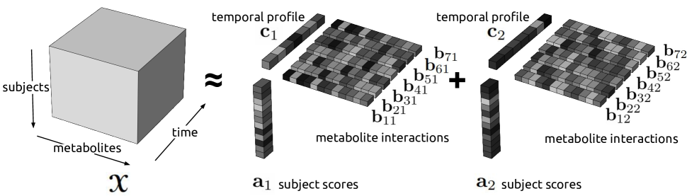
4.2 Simulated data analyis

Figure 3: FMS for all methods at different noise levels when compared with the ground truth factors. Each boxplot contains 20 points, one for the best-performing run of the method in each dataset. $\lambda$ denotes the strength of the ridge penalty imposed on all factors in the PARAFAC2 model or specifically to the factors ${\bm{\mathbf{{A}}}}$ and $\{{{\bm{\mathbf{{D}}}}}\}_{k=1}^{25}$ in the tPARAFAC2 model. $\lambda_{B}$ represents the strength of the temporal smoothness penalty.

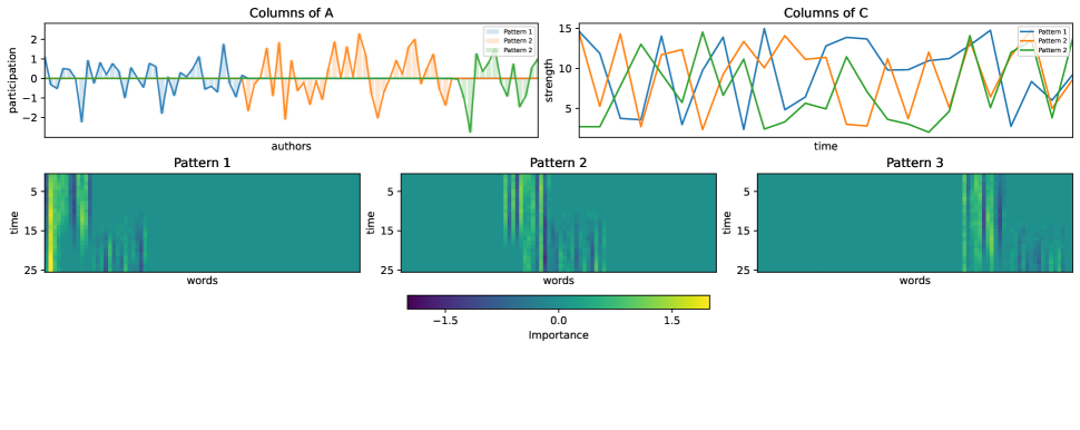
We first assess the performance of tPARAFAC2 on synthetic data. One potential use case would be to track evolving concepts across an $authors\times words\times time$ tensor. To generate such data, we generate ground truth factors ${\bm{\mathbf{{A}}}},\{{\bm{\mathbf{{B}}}}_{k}\}_{k=1}^{K}$ and $\{{\bm{\mathbf{{D}}}}_{k}\}_{k=1}^{K}$ that reflect the evolution of three concepts across time, and then form each temporal slice of the dataset as ${\bm{\mathbf{{X}}}}_{k}={\bm{\mathbf{{A}}}}{\bm{\mathbf{{D}}}}_{k}{\bm{\mathbf{{B}}}}_{k}^{{\sf T}},\ \forall k=1,...,K$ . Figure 2 shows the factors of such a dataset. Each concept consists of three parts:

1. A list of relevant authors participating in the concept. We simulate that by selecting a set of relevant author-indices for the respective column of factor ${\bm{\mathbf{{A}}}}$ and drawing ‘participation’ values from $\mathcal{N}(0,1)$, while the rest is set to $0$.

2. The words that compose each concept across time. This is captured by the non-zero indices of the respective column across all $\{{\bm{\mathbf{{B}}}}_{k}\}_{k=1}^{K}$ factors. For each concept, we randomly choose an initial and final word set, in which the concept has non-zero values at the first and last time step, respectively. The ‘importance’ values for the initial set are drawn from $\mathcal{N}(0,1)$. To model smooth evolution, we incrementally add a value from $\mathcal{N}(0,0.1)$ over time. After a randomly chosen time point, the concept begins to shift towards the final word set: with a probability of $0.3$, a word that is in the initial set but not in the final will start reducing to zero, or a new word from the final set will be initialized with a value from $\mathcal{N}(0,0.1)$ or both events occur. $30\%$ of the words of each concept will remain active at all times, as they are chosen to be in both the initial and final set.

3. The pattern’s strength (popularity) across time, reflected in ${\bm{\mathbf{{C}}}}$. We simulate that by drawing values from $\mathcal{U}(1,15)$. We make sure the congruence coefficient, i.e., the cosine similarity between columns, is no more than 0.8 in each generated dataset [21].

4.2.1 Different noise levels

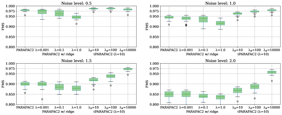
Here, we assess the performance of tPARAFAC2 in terms of accuracy on data with slowly changing patterns in the presence of different amounts of noise. We create 20 datasets of size $100\times 80\times 25$ that contain three concepts. After forming the data tensor $\bm{\mathscr{{X}}}$, we add noise as follows:

$$\bm{\mathscr{{X}}}_{noisy}=\bm{\mathscr{{X}}}+\eta\lVert\bm{\mathscr{{X}}}\rVert\frac{\Theta}{\lVert\Theta\rVert}$$ (20)

where $\Theta\sim\mathcal{N}(0,1)$ and $\eta\in\{0.5,1.0,1.5,2.0\}$ controlling the noise level. We compare PARAFAC2, PARAFAC2 with ridge regularization on all modes and tPARAFAC2 in terms of recovering the ground truth factors. All methods impose non-negativity on ${\bm{\mathbf{{C}}}}$ to alleviate the sign ambiguity, and AO-ADMM is used to fit the models. For each dataset, thirty random initializations are generated that are used by all methods. After discarding degenerate runs [36], we choose the best run for each method for each dataset according to the lowest loss function value.

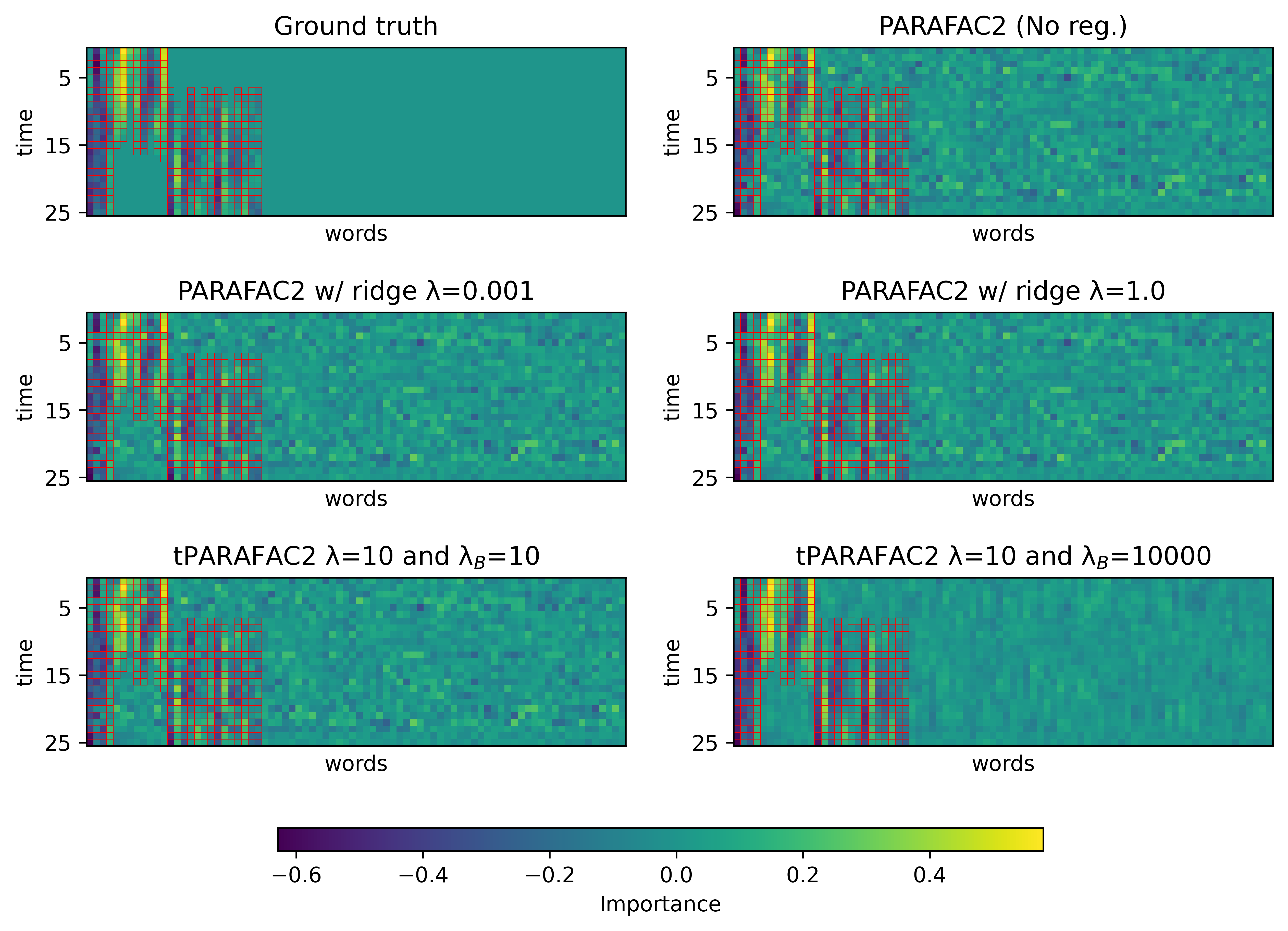
Figure 3 shows that as the noise level increases, tPARAFAC2 is able to recover the ground truth factors more accurately than other methods. We omit higher hyperparameters for ridge due to a consistent decline in accuracy. The main source of improvement for tPARAFAC2 is the increased accuracy of recovering ${\bm{\mathbf{{B}}}}_{k}$ factor matrices. An indicative example of why this is the case is shown in Figure 4. To illustrate this, we first concatenate all non-zero elements of the ground truth concept into a vector and then compute the cosine similarity with the vectors containing the respective entries from the reconstructions, as shown in Figure 4. Additionally, we can estimate the noise remaining in the factor by measuring the norm of the rest of the entries (i.e. non-active). Notice that the cosine similarity cannot be used here since the ground truth is a zero vector. A high norm indicates a noisy factor. We can see that tPARAFAC2 is more accurate because the temporal smoothness (a) helps recover the ground truth structure more accurately and (b) makes the method more robust to noise.

(a)

Method	Cosine sim. of ‘active’	Norm of ‘inactive’
PARAFAC2	0.90	2.81
PARAFAC2 w/ ridge $\lambda=0.001$	0.90	2.79
PARAFAC2 w/ ridge $\lambda=1$	0.90	2.79
tPARAFAC2 $\lambda=10$, $\lambda_{B}=10$	0.91	2.73
tPARAFAC2 $\lambda=10$, $\lambda_{B}=10000$	0.98	1.66

(b)

Figure 4: (a) depicts a slowly changing pattern, with the ‘active’ words marked in red. The second column of (b) shows the cosine similarity between vectors of ‘active’ words and the ground truth. The last column measures the norm of all non-active entries. These measurements are taken after normalizing the factors, with noise level $\eta=2.0$.

4.2.2 Randomly missing entries

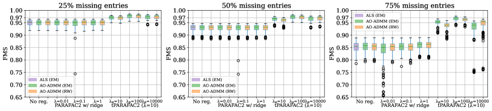
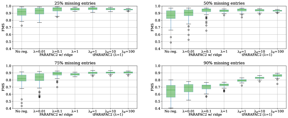
In this experiment, we assess the performance of tPARAFAC2 in terms of finding underlying slowly changing patterns in the presence of missing data. We construct 20 datasets with size $100\times 80\times 25$ and add noise with $\eta={0.75}$. For each of those datasets, we create $10$ binary tensor masks that indicate whether an entry is observed or not, with $25\%$, $50\%$ and $75\%$ entries set as missing. We compare the performace of PARAFAC2, PARAFAC2 with ridge regularization on all modes with strength $\lambda\in\{0.01,0.1,1.0\}$ and tPARAFAC2 with ridge hyperparameters being $\lambda=10$ and $\lambda_{B}\in\{10,100,1000\}$. We consider AO-ADMM (EM) and AO-ADMM (RW) for fitting these models. As another baseline, we also use the standard PARAFAC2-ALS (EM) approach for handling missing data [21]. For each mask, $30$ random initializations (the same 30 across all methods) are used. For EM-based approaches, we use the mean of the known entries of each frontal slice as the initial estimate of missing entries.

Figure 6(a) demonstrates the accuracy of each method in terms of recovering the ground truth factors. As the percentage of missing data increases, it gets increasingly difficult for methods to recover the underlying patterns. Our observations reveal that incorporating ridge regularization, in this case, does not enhance the recovery quality. However, tPARAFAC2 demonstrates superior ability to estimate the ground truth by leveraging the temporal smoothness imposed on the evolving factors, especially at $75\%$ missing data. Similar to the experiments with different amounts of noise, this improvement is attributed to tPARAFAC2’s (a) better ability to capture slowly changing patterns and (b) stronger noise reduction. We also note that there are outliers in tPARAFAC2 with $\lambda_{B}=10000$ in the $75\%$ missing data case. These are due to one of the patterns being almost completely missing, which results in the respective factors being “over smoothened”, and hence achieving low FMS.

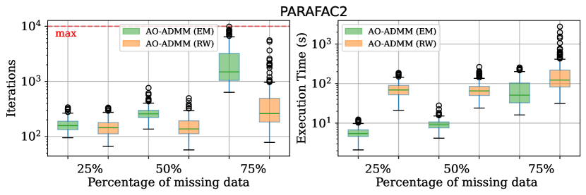
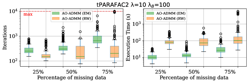
We also compare the two different ways of handling missing data using AO-ADMM when fitting PARAFAC2 and tPARAFAC2 models in terms of computational time (Figure 5). As the percentage of unobserved data increases, the problem’s difficulty increases, requiring more iterations and longer execution times. Furthermore, we observe that the AO-ADMM (EM) approach for fitting the models requires more iterations to converge than AO-ADMM (RW). However, each iteration is computationally less expensive, making the total execution time less. The primary computational bottleneck for the AO-ADMM (RW) method occurs during the update of the evolving mode factors, specifically the inversion of the term ${\bm{\mathbf{{D}}}}_{k}{\bm{\mathbf{{A}}}}^{{\sf T}}diag({\bm{\mathbf{{W}}}}(:,j)){\bm{\mathbf{{A}}}}{\bm{\mathbf{{D}}}}_{k}+\rho_{B_{k,j}}{\bm{\mathbf{{I}}}}$ across all indices $j$ and $k$ in (17). Moreover, adding temporal regularization increases computation time for datasets with $25\%$ and $50\%$ missing data. For datasets with $75\%$ missing data, temporal regularization slightly reduces the total execution time (compared to PARAFAC2).

Overall, these findings demonstrate that tPARAFAC2 is more accurate than PARAFAC2 for high amounts of missing data when the underlying patterns are slowly changing. Furthermore, the two approaches EM and RW for incorporating missing data yield similar accuracy; however, RW is computationally more intensive, making EM the preferable choice.

Experiments with higher percentages of missing data indicate that tPARAFAC2 consistently recovers the ground truth with higher accuracy and the improvement is even larger. Comparing the two approaches of incorporating missing data we notice similar results between EM and RW for tPARAFAC2. For PARAFAC2, however, we notice that RW completely fails to recover the ground truth under these conditions, with a median FMS of less than 0.2 over 200 runs, unless ridge (or temporal smoothness) regularization is imposed. The poor performance can be attributed to its update rules, specifically (16), (17), and (18). These rules require a sufficient number of data points or at least some prior knowledge through regularization, both of which are lacking in this setting.

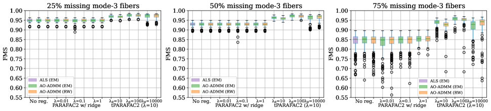
4.2.3 Structured missing data

Frequently, missing data has a specific structure, rather than being random as in the previous experimental setting. For example, relevant words of an author might be missing at certain time points or information about a particular word could be consistently missing for that author. Here, we assess the performance of methods in the presence of such structured missing data.

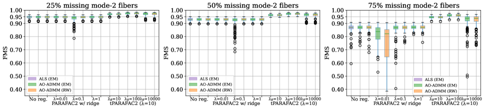
We generate $20$ datasets with dimensions $100\times 80\times 25$, introduce noise with $\eta={0.75}$ and then, for each dataset, apply $10$ binary indicator masks with $10\%$, $25\%$ and $40\%$ of mode-2 and mode-3 fibers fully missing. We do not consider mode-1 fibers missing as PARAFAC2 is not able to handle this case. We then fit PARAFAC2 to each dataset using both ALS and AO-ADMM. Comparisons are also made with PARAFAC2 models incorporating ridge regularization across all modes, and tPARAFAC2 models, which are computed using both EM and RW updates. As in the previous setups, $30$ initializations are shared across methods for each mask and each dataset.

Figures 6(b) and 6(c) show that, in general, as the amount of missing data increases, the quality of recovery for all methods decreases, although tPARAFAC2 demonstrates a smaller decline and outperforms both PARAFAC2 and PARAFAC2 with ridge regularization in all cases. Accuracy-wise, the two approaches of handling missing data within the PARAFAC2 AO-ADMM framework perform similarly. Nevertheless, the RW approach, as also observed in the previous experiment, has higher computation times. For PARAFAC2 with $\lambda=0.01$ in the $75\%$ missing mode-2 fibers case, we notice that using more initializations increases the accuracy of the results. Nonetheless, the results here only include the $30$ pre-generated initializations shared across all methods.

(a)

(b)

Figure 5: Comparison of EM and RW methods in terms of computation time. The measurements are taken on the runs of the randomly missing entries experimental setting and each boxplot contains 200 points, one for the best run of the respective method on each of the missing masks (10 for each dataset) of each dataset (20 total). (a) shows the results for PARAFAC2 while (b) the respective results for tPARAFAC2, where $\lambda=10$ and $\lambda_{B}=100$.

(a)

(b)

(c)

Figure 6: Accuracy of methods in terms of FMS with the ground truth. Each boxplot contains $200$ points, one for the best-performing run of the method at each mask of each dataset. (a) refers to randomly missing entries, (b) and (c) show the performance on structured missing data, i.e., mode-2 and mode-3 fibers fully missing, respectively.

4.3 Real data analysis

4.3.1 Chemometrics Application

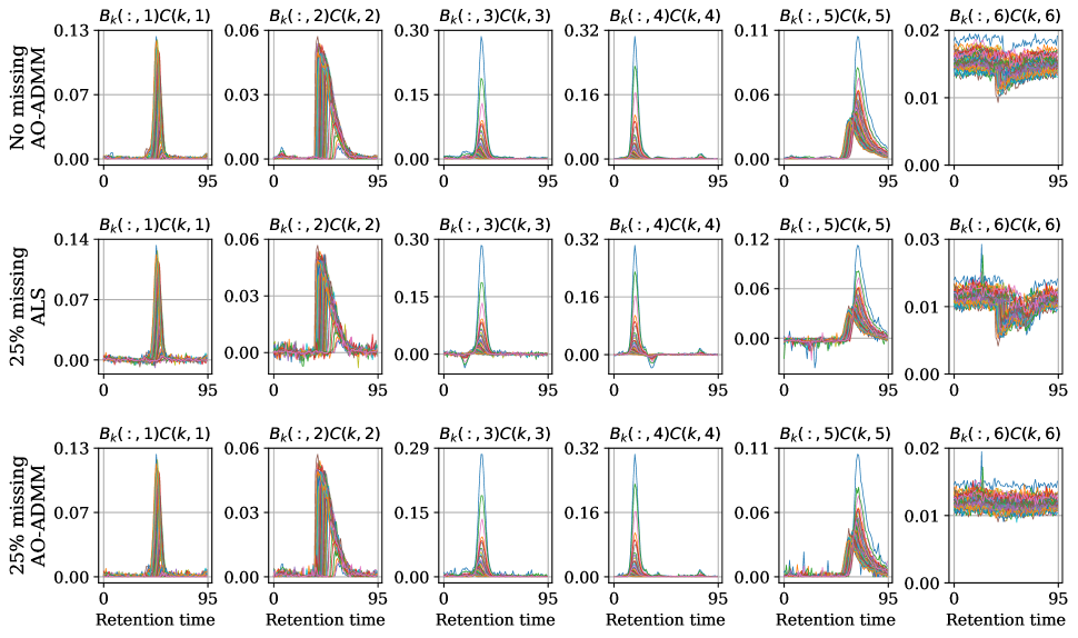
Here, we use GC-MS (Gas Chromatography-Mass Spectrometry) measurements of apple wine samples, and analyze the data using PARAFAC2 with the goal of revealing the composition of mixtures (i.e., wine samples). The dataset is in the form of a third-order tensor with modes: 286 mass spectra, 95 retention time, and 57 wine samples.

PARAFAC2 has shown to be an effective approach to analyze such data and identify the compounds in the samples since the model allows for retention time shifts of the compounds in different samples [17]. Previously, PARAFAC2 with non-negativity constraints on all modes has been fitted to this data using AO-ADMM, demonstrating how constraints improve the interpretability of the model [30]. Here, we demonstrate that constraints on the evolving mode improve the accuracy of the recovered patterns in the presence of missing data. The data is non-negative and we fit a 6-component PARAFAC2 model using AO-ADMM with non-negativity constraints on all modes. Each PARAFAC2 component reveals a mass spectrum (${{\bm{\mathbf{{A}}}}}$), elution profile ($\{{\bm{\mathbf{{B}}}}_{k}\}_{k=1}^{57}$) and the relative concentration of a chemical compound (modelled by this component) in the samples (${\bm{\mathbf{{C}}}}$). In order to assess the performance in the presence of missing data, we randomly generate $150$ binary indicator tensor masks ($50$ for $25\%$ missing data, $50$ for $50\%$ missing data, and $50$ for $75\%$ missing data) and compare the estimated patterns from data with missing entries using a PARAFAC2 model (fitted using ALS (EM) and AO-ADMM (EM)) with the patterns captured from the full data. When fitting PARAFAC2 using ALS (EM), we are only able to impose non-negativity on the first and third mode, while AO-ADMM imposes non-negativity constraints on all modes. For each mask, $50$ initializations are randomly generated that are shared between methods and we only consider the solution using the initialization that results in the lowest function value (Equation (5)).

Figure 7 shows the FMS values comparing the estimated factors from data with missing entries with the factors captured from the full data. We observe that incorporating the prior knowledge of the non-negativity of the factor improves the quality of the recovery. Thus, the AO-ADMM approach performs better. While both approaches achieve comparable accuracy in recovering the mass spectra ${\bm{\mathbf{{A}}}}$ and sample concentration ${\bm{\mathbf{{C}}}}$ factors, AO-ADMM demonstrates a distinct advantage in accurately recovering $\{{\bm{\mathbf{{B}}}}_{k}\}_{k=1}^{57}$ corresponding to elution profiles. Figure 9 shows the uncovered profiles scaled by their concentration when no missing entries exist, alongside the factors when $25\%$ of the input is missing (one of the $50$ masks). The profiles obtained via ALS exhibit negative peaks, which are not realistic and hinder interpretation. In contrast, the non-negativity constraint applied in the AO-ADMM approach enhances accuracy by eliminating unrealistic negative components. For the full data, we note that ALS has an FMS of 0.98 with the solution given by AO-ADMM.

4.3.2 Metabolomics Application

Figure 7: Chemometrics Application. Accuracy of extracted patterns from the GC-MS data using PARAFAC2 models measured by FMS with factors of fully observed data. Each boxplot contains 50 points, one for the best run of each method for each mask. ^∗: ALS has non-negativity constraints on the first and last modes, AO-ADMM on all three modes.

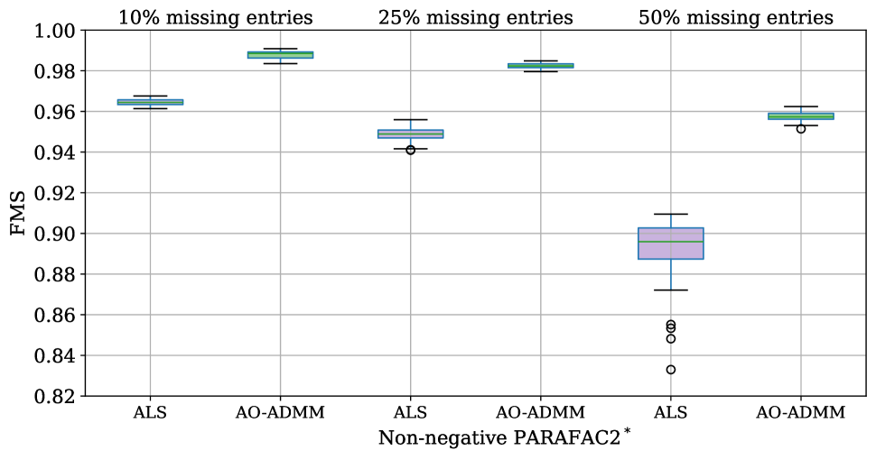
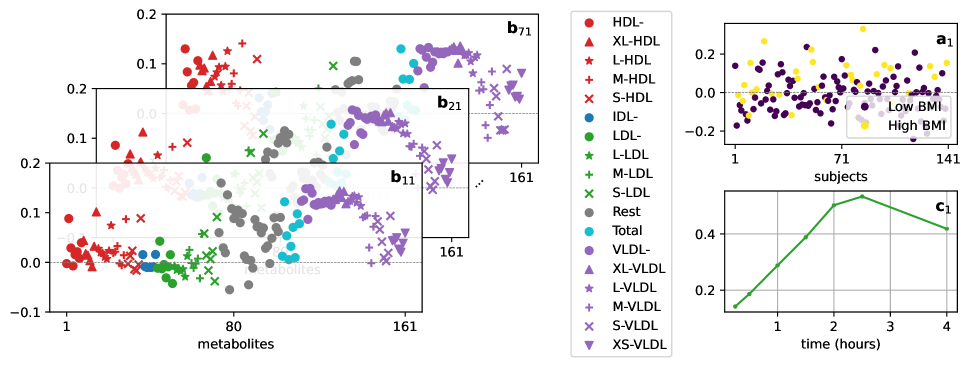
In this application, we analyze dynamic metabolomics data using a PARAFAC2 model to reveal evolving patterns in the metabolite mode. We also demonstrate the effect of temporal smoothness in the case of missing data. The dataset used in this experiment corresponds to Nuclear Magnetic Resonance (NMR) spectroscopy measurements and hormone measurements of blood samples collected during a meal challenge test from the COPSAC₂₀₀₀ (Copenhagen Prospective Studies on Asthma in Childhood) cohort [37]. Blood samples were collected from participants after overnight fasting and at regular intervals after the meal intake (15 min, 30 min, 1 hr, 1.5 hr, 2 hr, 2.5 hr and 4 hr). To investigate metabolic differences among subjects in response to a meal challenge, these measurements have previously been analyzed using a CP model, revealing biomarkers of a BMI (body mass index)-related phenotype as well as gender differences [38]. Here, we use the measurements from males arranged as a third-order tensor with modes: 140 subjects, 161 metabolites, 7 time points. See [38] for more details about sample collection and data preprocessing.

We analyze the data using a 2-component PARAFAC2 (and tPARAFAC2) model as in Figure 8 (where the number of components is selected based on the replicability of the components across subsets of subjects [38, 15]. For more details, see the Supplementary Material.) While the CP model reveals the same metabolite mode factor for all time slices, PARAFAC2 allows metabolite mode factors to change in time. The component revealing BMI-related group difference is shown in Figure 11. In the Supplementary Material, we also compare CP and PARAFAC2 in terms of correlations with other meta-variables of interest (in addition to BMI). All in all, PARAFAC2 and tPARAFAC2 reveal evolving metabolite patterns while keeping the correlations comparable to CP. An animation of evolving PARAFAC2 factors is given in the GitHub repo. Such evolving patterns reveal insights about the underlying mechanisms, e.g., the model captures the positive association between higher BMI and specific aminoacids, glycolysis-related metabolites, insulin and c-peptide at early time points - which disappears at later time points.

We also assess the performance of different models in the presence of missing data. Different amounts of missing data ($25\%$, $50\%$, $75\%$ and $90\%$) are introduced, and we attempt to recover the patterns captured from the fully observed data using a PARAFAC2 model (fitted with AO-ADMM). For each percentage of missing data, we randomly generate $50$ different indicator masks $\bm{\mathscr{{W}}}$, and for each mask $50$ different random initializations are used (shared across all methods). The best run for each method and each mask is selected based on the lowest function value across all initializations. When generating each mask, we make sure that no full slices (any mode) or any mode-1 fibers are missing, and additionally, we do not allow for mode-3 fibers to be missing since missing measurements for a single metabolite for a single subject across time does not make sense. Instead, half of the missing entries in this experiment originate from fully missing mode-2 fibers (e.g., all measurements for a single subject at a single time point are missing), while the rest are randomly missing entries. We compare PARAFAC2, PARAFAC2 with ridge on all modes and tPARAFAC2, where AO-ADMM is used to fit the models. Figure 10 shows that both ridge and temporal smoothness improve the recovery of the patterns, compared to PARAFAC2 without regularization. For PARAFAC2 with ridge, we notice that setting $\lambda=0.1$ or $\lambda=1$ consistently delivers accurate results that are comparable to tPARAFAC2. This changes, however, when $90\%$ of the data is missing, where tPARAFAC2 shows a clear improvement. However, we should note that such high amounts of missing data are not realistic in these measurements. Nevertheless, results are consistent with our experiments on simulated data: tPARAFAC2 enhances the recovery of underlying slowly changing patterns in temporal data, particularly for high levels of missingness.

Figure 8: 2-component PARAFAC2 model of the metabolomics data with modes: subjects, metabolites, and time.

Figure 9: Chemometrics Application. Recovered factors from the retention time mode scaled by sample coefficient when no data is missing (first row), when $25\%$ of the input is missing and ALS with non-negativity on the first and third mode is used to fit PARAFAC2 (second row), when $25\%$ of the input is missing and AO-ADMM with non-negativity on all modes is used to fit PARAFAC2 (third row). Each colored line corresponds to different values of $k$ (different samples).

Figure 10: Metabolomics Application. FMS is computed using the factors extracted from the full dataset. Each boxplot contains 50 points, one for each random mask generated for each percentage.

Figure 11: Metabolomics Application. The component showing statistically significant BMI group difference extracted from dynamic metabolomics data using PARAFAC2 (with non-negativity on the third mode). ${\bm{\mathbf{{b}}}}_{k1}$, for $k=1,...,7$ correspond to the factors in the metabolite mode changing in time. ${\bm{\mathbf{{a}}}}_{1}$ shows the subject coefficients where subjects are colored according to BMI groups, and ${\bm{\mathbf{{c}}}}_{1}$ shows the temporal profile. An animation of the evolving factors ${\bm{\mathbf{{b}}}}_{k1}$ can be found alongside our code.

5 Conclusion

In this paper, we introduced tPARAFAC2, a time-aware extension of the PARAFAC2 model, that involves temporal regularization, and fitted the model using an AO-ADMM-based algorithm. As temporal data is frequently incompletely observed, we introduced two approaches for handling missing data within the PARAFAC2 AO-ADMM framework. Numerical experiments on both synthetic and real datasets demonstrate the effectiveness of the EM-based approach for handling missing data, and also show that tPARAFAC2 outperforms PARAFAC2 and PARAFAC2 with ridge in terms of recovering the underlying slowly changing patterns, especially when a large percentage of the input data is missing.

While the PARAFAC2 constraint has been crucial for uniquely capturing evolving patterns, we plan to study whether the constraint can be omitted when temporal data is jointly analyzed with other data sets [39] and revisit CMF-based approaches that have previously shown to suffer from uniqueness issues [27]. Furthermore, we will also study hyperparameter selection using the replicability of the extracted patterns.

References

- [1] E. Acar, M. Roald, K. M. Hossain, V. D. Calhoun, and T. Adali, “Tracing evolving networks using tensor factorizations vs. ICA-based approaches,” Frontiers in Neuroscience, vol. 16, p. 861402, 2022.
- [2] M. Ahn, N. Eikmeier, J. Haddock, L. Kassab, A. Kryshchenko, K. Leonard, D. Needell, R. W. M. Madushani, E. Sizikova, and C. Wang, On Large-Scale Dynamic Topic Modeling with Nonnegative CP Tensor Decomposition, pp. 181–210. Advances in Data Science, 2021.
- [3] B. W. Bader, M. W. Berry, and M. Browne, “Discussion tracking in enron email using PARAFAC,” in Survey of Text Mining: Clustering, Classification, and Retrieval, 2nd ed., pp. 147–162, Springer, 2007.
- [4] R. A. Harshman, “Foundations of the PARAFAC procedure: Models and conditions for an ”explanatory” multi-modal factor analysis,” UCLA Working Papers in Phonetics, vol. 16, pp. 1–84, 1970.
- [5] J. D. Carroll and J.-J. Chang, “Analysis of individual differences in multidimensional scaling via an n-way generalization of “eckart-young” decomposition,” Psychometrika, vol. 35, pp. 283–319, 1970.
- [6] W. Zhang, H. Sun, X. Liu, and X. Guo, “Temporal QoS-aware web service recommendation via non-negative tensor factorization,” in Proceedings of the 23rd Int. Conf. World Wide Web, p. 585–596, 2014.
- [7] H.-F. Yu, N. Rao, and I. S. Dhillon, “Temporal regularized matrix factorization for high-dimensional time series prediction,” in Advances in Neural Information Processing Systems, vol. 29, pp. 847–855, 2016.
- [8] D. Ahn, J. Jang, and U. Kang, “Time-aware tensor decomposition for sparse tensors,” Mach. Learn., vol. 111, no. 4, pp. 1409–1430, 2022.
- [9] R. Pasricha, E. Gujral, and E. E. Papalexakis, “Identifying and alleviating concept drift in streaming tensor decomposition,” in ECML PKDD: Proc. European Conf. Machine Learning and Knowledge Discovery in Databases, p. 327–343, 2019.
- [10] A. P. Singh and G. J. Gordon, “Relational learning via collective matrix factorization,” in KDD: Proc. 14th ACM SIGKDD Int. Conf. Knowledge Discovery and Data Mining, p. 650–658, 2008.
- [11] W. Yu, C. C. Aggarwal, and W. Wang, “Temporally factorized network modeling for evolutionary network analysis,” in Proc. Tenth ACM Int. Conf. Web Search and Data Mining, p. 455–464, 2017.
- [12] A. P. Appel, R. L. F. Cunha, C. C. Aggarwal, and M. M. Terakado, “Temporally evolving community detection and prediction in content-centric networks,” in ECML PKDD: Proc. European Conf. Machine Learning and Knowledge Discovery in Databases, pp. 3–18, 2019.
- [13] B. Hooi, K. Shin, S. Liu, and C. Faloutsos, “SMF: drift-aware matrix factorization with seasonal patterns,” in SDM: Proc. SIAM Int. Conf. Data Mining, pp. 621–629, 2019.
- [14] K. Kawabata, S. Bhatia, R. Liu, M. Wadhwa, and B. Hooi, “SSMF: shifting seasonal matrix factorization,” Advances in Neural Information Processing Systems, vol. 34, pp. 3863–3873, 2021.
- [15] T. Adali, F. Kantar, M. A. B. S. Akhonda, S. Strother, V. D. Calhoun, and E. Acar, “Reproducibility in matrix and tensor decompositions: Focus on model match, interpretability, and uniqueness,” IEEE Signal Processing Magazine, vol. 39, no. 4, pp. 8–24, 2022.
- [16] R. A. Harshman, “PARAFAC2: Mathematical and technical notes,” UCLA Working Papers in Phonetics, no. 22, pp. 30–47, 1972.
- [17] R. Bro, C. A. Andersson, and H. A. Kiers, “PARAFAC2—part ii. modeling chromatographic data with retention time shifts,” Journal of Chemometrics, vol. 13, no. 3-4, pp. 295–309, 1999.
- [18] K. H. Madsen, N. W. Churchill, and M. Mørup, “Quantifying functional connectivity in multi-subject fMRI data using component models: Quantifying functional connectivity,” Human Brain Mapping, vol. 38, pp. 882–899, Oct. 2017.
- [19] I. Lehmann, E. Acar, T. Hasija, M. Akhonda, V. D. Calhoun, P. J. Schreier, and T. Adali, “Multi-task fMRI data fusion using IVA and PARAFAC2,” in ICASSP: Proc. IEEE Int. Conf. Acoustics, Speech and Signal Processing, pp. 1466–1470, 2022.
- [20] I. Perros, E. E. Papalexakis, R. Vuduc, E. Searles, and J. Sun, “Temporal phenotyping of medically complex children via PARAFAC2 tensor factorization,” Journal of Biomedical Informatics, vol. 93, p. 103125, 2019.
- [21] H. A. L. Kiers, J. M. F. ten Berge, and R. Bro, “PARAFAC2—Part I. A direct fitting algorithm for the PARAFAC2 model,” Journal of Chemometrics, vol. 13, no. 3-4, pp. 275–294, 1999.
- [22] K. Yin, A. Afshar, J. C. Ho, W. K. Cheung, C. Zhang, and J. Sun, “LogPar: Logistic PARAFAC2 factorization for temporal binary data with missing values,” in KDD: Proc. 26th ACM SIGKDD Int. Conf. Knowledge Discovery & Data Mining, pp. 1625–1635, 2020.
- [23] A. Afshar, I. Perros, E. E. Papalexakis, E. Searles, J. Ho, and J. Sun, “COPA: Constrained parafac2 for sparse & large datasets,” in CIKM: Proc. 27th ACM Int. Conf. Information and Knowledge Management, pp. 793–802, 2018.
- [24] Y. Ren, J. Lou, L. Xiong, and J. C. Ho, “Robust irregular tensor factorization and completion for temporal health data analysis,” in CIKM: Proc. 29th ACM Int. Conf. Information & Knowledge Management, pp. 1295–1304, 2020.
- [25] J.-G. Jang, J. Lee, J. Park, and U. Kang, “Accurate PARAFAC2 decomposition for temporal irregular tensors with missing values,” in 2022 IEEE Int. Conf. Big Data, pp. 982–991, 2022.
- [26] K. Yin, W. K. Cheung, B. C. M. Fung, and J. Poon, “TedPar: Temporally dependent PARAFAC2 factorization for phenotype-based disease progression modeling,” in SDM: Proc. SIAM Int. Conf. Data Mining, pp. 594–602, 2021.
- [27] C. Chatzis, M. Pfeffer, P. Lind, and E. Acar, “A time-aware tensor decomposition for tracking evolving patterns,” in MLSP: Proc. IEEE 33rd Int. Workshop Machine Learning for Signal Processing, pp. 1–6, 2023.
- [28] T. G. Kolda and B. W. Bader, “Tensor decompositions and applications,” SIAM Review, vol. 51, no. 3, pp. 455–500, 2009.
- [29] J. E. Cohen and R. Bro, “Nonnegative PARAFAC2: A flexible coupling approach,” in LVA/ICA: Proc. Int. Conf. Latent Variable Analysis and Signal Separation, pp. 89–98, 2018.
- [30] M. Roald, C. Schenker, V. D. Calhoun, T. Adali, R. Bro, J. E. Cohen, and E. Acar, “An AO-ADMM approach to constraining PARAFAC2 on all modes,” SIAM Journal on Mathematics of Data Science, vol. 4, no. 3, pp. 1191–1222, 2022.
- [31] M. Roald, S. Bhinge, C. Jia, V. Calhoun, T. Adalı, and E. Acar, “Tracing network evolution using the PARAFAC2 model,” in ICASSP: Proc. IEEE Int. Conf. Acoustics, Speech and Signal Processing, pp. 1100–1104, 2020.
- [32] A. P. Dempster, N. M. Laird, and D. B. Rubin, “Maximum likelihood from incomplete data via the EM algorithm,” Journal of the Royal Statistical Society Series B: Statistical Methodology, vol. 39, no. 1, pp. 1–22, 1977.
- [33] K. Huang, N. D. Sidiropoulos, and A. P. Liavas, “A flexible and efficient algorithmic framework for constrained matrix and tensor factorization,” IEEE Transactions on Signal Processing, vol. 64, no. 19, pp. 5052–5065, 2016.
- [34] J. Kossaifi, Y. Panagakis, A. Anandkumar, and M. Pantic, “Tensorly: Tensor learning in python,” Journal of Machine Learning Research, vol. 20, no. 26, 2019.
- [35] M. Roald, “Matcouply: Learning coupled matrix factorizations with python,” SoftwareX, vol. 21, p. 101292, 2023.
- [36] B. J. H. Zijlstra and H. A. L. Kiers, “Degenerate solutions obtained from several variants of factor analysis,” Journal of Chemometrics, vol. 16, no. 11, pp. 596–605, 2002.
- [37] H. Bisgaard, “The Copenhagen prospective study on asthma in childhood (copsac): design, rationale, and baseline data from a longitudinal birth cohort study,” Annals of Allergy, Asthma & Immunology, vol. 93, no. 4, pp. 381–389, 2004.
- [38] S. Yan, L. Li, D. Horner, P. Ebrahimi, B. Chawes, L. O. Dragsted, M. A. Rasmussen, A. K. Smilde, and E. Acar, “Characterizing human postprandial metabolic response using multiway data analysis,” Metabolomics, vol. 20, no. 3, p. 50, 2024.
- [39] C. Schenker, J. E. Cohen, and E. Acar, “A flexible optimization framework for regularized matrix-tensor factorizations with linear couplings,” IEEE Journal of Selected Topics in Signal Processing, vol. 15, no. 3, pp. 506–521, 2021.