Hyperspectral Pansharpening: Critical Review, Tools and Future Perspectives

Abstract

Hyperspectral pansharpening consists of fusing a high-resolution panchromatic band and a low-resolution hyperspectral image to obtain a new image with high resolution in both the spatial and spectral domains. These remote sensing products are valuable for a wide range of applications, driving ever growing research efforts. Nonetheless, results still do not meet application demands. In part, this comes from the technical complexity of the task: compared to multispectral pansharpening, many more bands are involved, in a spectral range only partially covered by the panchromatic component and with overwhelming noise. However, another major limiting factor is the absence of a comprehensive framework for the rapid development and accurate evaluation of new methods. This paper attempts to address this issue.

We started by designing a dataset large and diverse enough to allow reliable training (for data-driven methods) and testing of new methods. Then, we selected a set of state-of-the-art methods, following different approaches, characterized by promising performance, and reimplemented them in a single PyTorch framework. Finally, we carried out a critical comparative analysis of all methods, using the most accredited quality indicators. The analysis highlights the main limitations of current solutions in terms of spectral/spatial quality and computational efficiency, and suggests promising research directions.

To ensure full reproducibility of the results and support future research, the framework (including codes, evaluation procedures and links to the dataset) is shared on https://github.com/matciotola/hyperspectral_pansharpening_toolbox, as a single Python-based reference benchmark toolbox.

I Introduction

High resolution is the most desired feature in a remote sensing image. High spatial resolution enables precise detection of objects and structures. High spectral resolution allows for the accurate classification of land covers. Unfortunately, there is a trade-off between these desirable properties. To obtain images with good signal-to-noise ratio, sufficient energy must be received in each acquisition cell, and this requires bigger ground samples or large acquisition bandwidths (or both). Modern optical systems overcome this limitation by acquiring two complementary pieces of information at the same time, a single-band panchromatic (PAN) image with high spatial resolution and a multiband image with lower spatial resolution. A pansharpening algorithm is then used to fuse them into a new single image featuring the desired high resolution in both domains.

Pansharpening has been the object of intense research in recent years. The most studied case is that of multispectral (MS) pansharpening, which involves a limited number of bands, usually from 4 to 8, in the visible to near-infrared spectrum. Extensive surveys on the topic can be found in the literature [1, 2, 3]. Recently, there has been a steadily growing interest in hyperspectral (HS) pansharpening, also testified by actions such as the HS pansharpening challenge [4]. HS images comprise hundreds of very narrow bands, covering collectively a large spectral range, going from 400 to 2500 nm. As a result, they provide very fine-scale information on a wide variety of phenomena, thereby holding great potential for several key applications in remote sensing, from classification [5, 6] and object detection [7, 8, 9] to land use/cover mapping [10, 11], crop monitoring [12, 13] and estimation of land physical parameters [14, 15].

From a technical point of view, HS pansharpening is a very challenging problem because of the large resolution mismatch between PAN and HS components and the low signal-to-noise ratio involved. The solutions designed for MS pansharpening certainly represent a good starting point also for the HS case and their extension is often simple. However, the notable differences between the two cases imply additional challenges that must be taken into account to prevent this naive reuse:

• PAN and MS data cover approximately the same spectral range (visible to near-infrared) and the PAN bandwidth encloses most MS bands. On the contrary, the spectral range of HS data goes well beyond that of the PAN (see Fig. 1) and a large number of HS bands, often the majority of them, do not overlap with the PAN. This means that, unlike for MS pansharpening, the PAN does not allow reliable prediction of the fine spatial structure of these bands. Likewise, they should not be considered in any procedure for PAN image estimation.

  

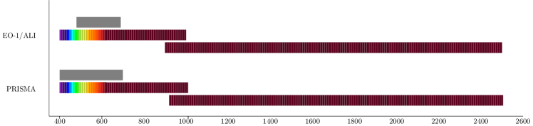
  Figure 1: Spectral range of HS (colored bars) and PAN (gray bar) sensors for EO-1/ALI and PRISMA sensing systems. Both are equipped with two partially overlapped spectrometers.

• Because HS bands are very narrow, on the order of 10 nm, large ground cells must be used to harvest sufficient energy, typically 30m or more. Nonetheless, the acquired data are rather noisy, and some bands or groups of bands must be discarded immediately because they are affected by acquisition errors and even the remaining ones may not have constant quality. Furthermore, there is a large resolution mismatch with the PAN, say, 30m vs. 5m, with a large amount of missing information that the pansharpening tool is called upon to recover.

• HS images are huge. Even assuming that complexity grows linearly with the number of bands, the computational burden of pansharpening is much larger than with MS images. Moreover, solutions based on machine learning require comparably large volumes of data for training, which may simply not be available.

The first HS pansharpening methods proposed in the literature, beginning with the 2007 paper by Aiazzi et al. [16], were indeed ingenious adaptations of solutions originally conceived for the MS case. In the following years, many more proposals considered the same path, with approaches based on Bayesian models [17, 18, 19, 20], matrix factorization [21, 22, 23], variational optimization [24], component substitution and multiresolution analysis [25] (see also the 2015 review by Loncan et al. [26]). Some methods specifically designed for HS pansharpening were also proposed, based on guided filtering [27], variational optimization [28, 29], saliency-based component substitution [30].

In the meantime, however, the deep learning (DL) revolution had already hit the field of remote sensing. Starting from the 2016 seminal work by Masi et al. [31], deep learning is by now a de-facto standard for both MS [32, 3, 33] and HS [34, 35, 36, 37] pansharpening. Limiting the analysis to the latter case, in [34] and [38] dedicated convolutional neural networks (CNNs) were designed to strengthen the spectral prediction capability. In [35], instead, a dual-attention residual network was proposed, with a deep HS image prior module for HS upsampling. In [39, 40] the problem of scale and resolution variability was tackled, by means of a CNN with arbitrary-scale attention modules [40]. An overcomplete residual network that learns high-level features using constrained receptive fields was proposed in [36]. Multibranch network architectures were also explored in several recent works [41, 42, 43]. Other methods adopted classical pansharpening paradigms and used DL modules to estimate the model parameters [44] or to process the extracted features [45]. All the above methods use supervised learning and perform training at reduced resolution using a subsampled version of the original data as ground truth (GT). Recently, to avoid the quality loss induced by subsampling, a paradigm shift towards full-resolution training is taking place for both MS [46, 47, 48] and HS [49, 37, 50] pansharpening, with novel unsupervised learning strategies and suitably defined loss functions.

This quick analysis shows growing research activity on HS pansharpening, with contributions primarily focused on DL-based methods. Performance, however, does not appear to be improving at a comparable rate, and the success seen in related fields is only coming slowly. A first reason for this failure is the scarcity and excessive heterogeneity of the data available to the scientific community, a well-known plague of remote sensing. Limiting the scope to the DL-oriented papers mentioned before, we observe that different research groups work on datasets that are small and incompatible with one another, acquired by different sensors, characterized by different spectral ranges, with different numbers of bands and different PAN-HS resolution ratios. A further problem is that the experimental protocols and metrics themselves used for performance evaluation often vary as well. Things are even worse for DL-based methods; virtually all new proposals these days need to be trained on large, high-quality datasets to express their full potential. Under these conditions, a new proposal can hardly be compared to previous ones based on numerical performance indicators, nor will it work on different data, unless properly adapted and retrained. All these problems represent major obstacles to scientific progress in this field.

This work tackles the above issues by providing a reliable framework that will help develop and assess new solutions for HS pansharpening. We begin by scanning the literature to identify a set of benchmark state-of-the-art (SoTA) methods. Our analysis follows an operational approach, focusing on methods that provide promising experimental results in some respect and can be faithfully replicated. After this phase, we build a new development and testing toolbox. We first assemble a large dataset of high-quality PAN+HS images to enable the reliable and uniform performance assessment of all methods and to support the accurate training of DL-based methods. Then, we re-implement all the selected methods in Python (retraining the DL models) and assess their performance both at reduced resolution and full resolution using the most accredited metrics in the literature. Eventually, we provide the community with an easy-to-use toolbox comprising data, tools, and results that we hope will simplify the development of new solutions and drive progress in this field. As far as we know, this is the first attempt to provide a critical comparison for the HS pansharpening problem. A unique instance of review fully devoted to HS pansharpening is in [26] but referring to dated approaches without involving DL solutions. Moreover, in [26], the assessment has been performed using simulated data (including simulated PANs) and just at reduced resolution. Instead, in this work, real data (both HS and PAN) are exploited, and the validation relies upon both reduced resolution and full resolution procedures.

According to this plan, the remainder of the paper is organized as follows: Section II provides a review of HS pansharpening solutions, with a special focus on those more amenable to be implemented and assessed; Section III describes the proposed approach to quality assessment; Section IV reviews the datasets used so far in HS pansharpening and describes the newly proposed dataset; Section V presents and discusses numerical and visual experimental results both at reduced and full resolution, extracting general guidelines for future work. Finally Section VI draws conclusions and outlines future work.

II Methods

TABLE I: HS pansharpening methods.

Name	Ref	Summary
EXP		Approximation of the ideal interpolator
Component Substitution (CS) methods
GSA	[51]	Gram-Schmidt adaptive component substitution
BT-H	[52]	Brovey transform with haze correction
BDSD-PC	[53]	Band-dependent spatial detail injection with physical constraint
PRACS	[54]	Partial replacement adaptive CS
Multiresolution Analysis (MRA) methods
MTF-GLP-FS	[55]	Modulation Transfer Function (MTF)-matched Generalized Laplacian Pyramid (MTF-GLP) with fusion rule at full scale
MTF-GLP-HPM	[56]	MTF-GLP with high pass modulation
MTF-GLP-HPM-R	[57]	MTF-GLP-HPM with regression-based spectral matching
AWLP	[58]	Additive wavelet luminance proportional
MF	[59]	Nonlinear decomposition with morphological filters
Model-Based Optimization (MBO) methods
HySURE	[18]	Bayesian estimation with vector total variation prior
SR-D	[60]	Sparse representations-based detail injection
TV	[61]	Total variation-based pansharpening
Deep Learning (DL) methods
HyperPNN	[34]	7-layer net with spectral encoder-decoder structure
HSpeNet	[38]	Advanced version of HyperPNN, with deeper architecture and Spectral Angle Mapper (SAM) loss term
DHP-DARN	[35]	Deep residual channel-spatial attention net with Deep Image Prior (DIP) for HS resizing
DIP-HyperKite	[36]	Overcomplete net with DIP for HS resizing
HyperDSNet	[62]	Spectral attention-based detail injection from deep-shallow features
R-PNN (unsup.)	[37]	Band-wise pansharpening using modified Z-PNN [47] with tuning propagation
PCA-Z-PNN (unsup.)	[50]	Z-PNN model with PCA-based input reduction

TABLE II: Main symbols used in the paper.

Symbol	Dimensions	Meaning
$R$	Scalar	Resolution ratio
$B$	Scalar	# of HS bands
$w,h$	Scalars	HS width and height, respectively
$W,H$	Scalars	PAN width and height, respectively
$\mathbf{H}$	$[w{\times}h{\times}B]$	Original HS image
$\mathbf{P}$	$[W{\times}H]$	Original PAN image
$\widetilde{\mathbf{H}}$	$[W{\times}H{\times}B]$	$R{\times}R$ upscaling of $\mathbf{H}$
$\widehat{\mathbf{H}}$	$[W{\times}H{\times}B]$	Pansharpening of $\mathbf{H}$
$\widetilde{\mathbf{X}}$ or $\widehat{\mathbf{X}}$	$[W{\times}H{\times}\ast]$	Upscaling or pansharpening of any $\mathbf{X}$

This section reviews SoTA solutions for HS pansharpening. However, rather than providing an exhaustive list of all papers published on this topic, we focus on a subset of representative methods, selected because they a) are distinctive from the methodological point of view; b) are competitive in terms of quality and/or computational efficiency; c) come with a publicly available software code (in any programming language) or are described with sufficient detail to be coded anew. All of them have been re-implemented (and assessed) in this work and eventually released as part of the proposed benchmarking toolbox.

Tab. I summarizes these methods, grouped according to the usual [2] categories of Component Substitution (CS), Multi-Resolution Analysis (MRA), Model-Based Optimization (MBO) which extends the usual Variational Optimization class, and DL. In the pansharpening literature, in addition to the fusion methods it is also custom to provide the simple expansion (EXP) of the HS (with no fusion with the PAN) obtained by an approximation of the ideal interpolator. This because such a product is a latent variable of many methods and represents a spectral benchmark. In the upcoming description, we will use the symbols recalled in Tab. II.

II-A Component substitution

The methods [1, 2, 26] are based on the use of a suitable transformation that brings the data to a domain where spatial and spectral components can be easily separated. Then, the spatial component is replaced by the available PAN and the data are transformed back into the original domain. By using a linear transformation and considering the substitution of a single component, a fast pansharpening process is obtained [63]. These techniques were initially proposed for MS pansharpening and, subsequently, extended to the HS case. Preliminarily, the HS datacube $\mathbf{H}\in\mathbb{R}^{w{\times}h{\times}B}$ is spatially resized to match the target pansharpening scale using (a polynomial approximation of) the ideal interpolator [1], yielding $\widetilde{\mathbf{H}}\in\mathbb{R}^{W{\times}H{\times}B}$. The component to be replaced, $\mathbf{I}\in\mathbb{R}^{W{\times}H}$, is obtained through a simple linear combination of the upscaled bands $\{\mathbf{H}^{b}\}$ of $\widetilde{\mathbf{H}}$, through suitably defined weights $\mathbf{w}=[w_{1},\ldots,w_{B}]^{T}$:

$$\mathbf{I}=\sum_{b=1}^{B}w_{b}\widetilde{\mathbf{H}}^{b}.$$ (1)

Both $\mathbf{P}$ and $\mathbf{I}$ are defined in the panchromatic domain and their difference, after histogram equalization, represents the high-frequency details missing in the original image. Therefore, the pansharpened bands $\{\widehat{\mathbf{H}}^{b}\}$ of $\widehat{\mathbf{H}}\in\mathbb{R}^{W{\times}H{\times}B}$ are obtained by injecting these details in the upscaled HS bands, weighted by suitable coefficients, the injection gains $\mathbf{g}=[g_{1},\ldots,g_{B}]$

$$\widehat{\mathbf{H}}^{b}=\widetilde{\mathbf{H}}^{b}+g_{b}(\mathbf{P}-\mathbf{I}),\;\;\;b=1,\ldots,B,$$ (2)

By changing the transformation, different combinations of injection gains and weights are needed.

II-A1 GSA

A powerful example of the CS approach is based on the orthogonal Gram-Schmidt (GS) decomposition of $\mathbf{H}$ [64]. Different variants can be obtained by changing the definition of the first component of the decomposition, the one to be replaced. The basic implementation proposed in [64] employs a simple uniform average: $w_{b}=1/B,\,\forall b$. The component substitution is then completed by inverting the orthogonal decomposition using the injection gains:

$$g_{b}=\frac{{\rm Cov}(\widetilde{\mathbf{H}}^{b},\mathbf{I})}{{\rm Var}(\mathbf{I})},\;\;b=1,\ldots,B,$$ (3)

where ${\rm Cov}(\cdot)$ and ${\rm Var}(\cdot)$ indicate the covariance and variance operators, respectively. This solution, however, does not take into account the different levels of correlation between $\mathbf{P}$ and each individual band of $\mathbf{H}$, giving rise to heavy spectral distortion. For this reason, a more robust variant, known as Gram-Schmidt Adaptive (GSA), was proposed in [65] for MS pansharpening and later applied to the HS case [25]. The latter is the first method selected for our experimental assessment. GSA differs from the classical GS implementation in that the weights $\{w_{b}\}$ used to compute $\mathbf{I}$ are not all equal but are estimated by minimizing the mean square error between $\mathbf{I}$ and a spatially degraded version of the PAN image.

II-A2 BT-H

Another CS method considered in this work is BT-H [52], which relies on an improved version of the Brovey Transform (BT) [66] that accounts for haze. In this case, space-variant injection gains are used, defined as

$$\mathbf{G}^{b}_{n}=\frac{\widetilde{\mathbf{H}}^{b}_{n}-h^{b}}{\mathbf{I}_{n}-h},\;\;\;\forall\,n,$$ (4)

where the ratio is meant to be pixel-wise, $n$ indicates the pixel location, $h^{b}$ the haze in the $b$-th HS band and $h$ is the haze in both $\mathbf{P}$ and $\mathbf{I}$. Of course, the product between the gains and $(\mathbf{P}-\mathbf{I})$ in Eq. 2 must be pixel-wise as well. The weights $\mathbf{w}$ are estimated by minimizing the mean square error between $\mathbf{I}$ and a reduced resolution version of $\mathbf{P}$.

II-A3 BDSD-PC

In [67] both weights $\mathbf{w}$ and gains $\mathbf{g}$ are obtained by minimizing the mean squared distance between the fused image given by Eq. 2 and the reference (GT) pansharpened image. Since the latter is not available, the optimization problem is shifted to the reduced resolution domain by means of a suitable scaling of the input images. This approach, known as Band-Dependent Spatial-Detail (BDSD) injection method [67], is here considered in the version proposed in [53] where a Physical Constraint is introduced (BDSD-PC) to regularize the estimation of the coefficients.

II-A4 PRACS

The last CS solution considered in our study is the Partial Replacement Adaptive Component Substitution (PRACS) [54], where the replacement of $\mathbf{I}$ is done, band-wise, with a suited weighted sum of $\mathbf{P}$ and $\widetilde{\mathbf{H}}^{b}$ rather than just using $\mathbf{P}$.

In general, CS methods are characterized by high spatial fidelity, low processing time, and robustness to registration errors and aliasing [68, 1]. On the downside, they tend to introduce significant spectral distortion due to the spectral mismatch between $\mathbf{P}$ and $\mathbf{H}$ [69]. This becomes a rather serious issue in the HS case, as opposed to the MS case, because of the large number of spectral bands that present little or no correlation with the PAN.

II-B Multiresolution analysis

Methods based on Multi-Resolution Analysis (MRA) [1, 2, 26] are formally very similar to CS methods, as they also involve the injection of spatial details in HS upscaled bands:

$$\widehat{\mathbf{H}}^{b}=\widetilde{\mathbf{H}}^{b}+\mathbf{G}^{b}\cdot(\mathbf{P}-\mathbf{P}^{\rm lp}),\;\;\;b=1,\ldots,B,$$ (5)

The fundamental difference is in how these spatial details, or so-called PAN details, are extracted. In MRA, they are computed as the difference between $\mathbf{P}$ and its low-pass filtered version, $\mathbf{P}^{\rm lp}$, while in CS as the difference between $\mathbf{P}$ and a weighted average of $\widetilde{\mathbf{H}}$ along the spectral dimension. The use of different filtering strategies and injection rules gives rise to different MRA solutions. SoTA injection schemes follow two approaches [70], commonly referred to as projective and multiplicative or high pass modulation (HPM). The former uses spatially constant gains $\mathbf{G}^{b}$, while the latter allows them to vary spatially so that the injection of detail can be modulated in the spatial domain. In more detail, the HPM injection gains are defined as $\mathbf{G}^{b}_{n}=\widetilde{\mathbf{H}}^{b}_{n}/\mathbf{P}^{\rm lp}_{n},\forall n$, with the goal of reproducing the local intensity contrast of the PAN image [70]. Different MRA techniques, however, are characterized mainly by how the PAN image is low-pass filtered.

II-B1 Laplacian-based techniques: MTF-GLP-*

A popular option is to use a Gaussian filter matched with the Modulation Transfer Function (MTF) of the high spectral resolution sensor, usually designed based on information provided by the manufacturer, such as the gains at the Nyquist frequency. In the context of multiresolution decomposition, this approach is usually called Generalized Laplacian Pyramid (GLP), since the desired detail $(\mathbf{P}-\mathbf{P}^{\rm lp})$ is approximated by Laplacian filtering.

In this work, we consider several SoTA techniques belonging to this category. The MTF-GLP-FS method is based on the Full Scale (FS) projective injection rule proposed in [55] working directly at full resolution. It has proven especially valuable in fusion problems characterized by a large resolution ratio. The classical multiplicative injection model is considered in MTF-GLP-HPM [25], implemented with suitable histogram matching to account for possible spectral distortions. Another variant of the multiplicative injection rule is introduced in MTF-GLP-HPM-R [57]. Here, the “R” stands for regression, because the spectral matching between each $\widetilde{\mathbf{H}}^{b}$ and $\mathbf{P}^{\rm lp}$ is achieved employing multivariate linear regression, better motivated than the classical histogram matching procedure under a physical point of view [57].

II-B2 AWLP

Other solutions are based on the wavelet transform. One of the most popular is the Additive Wavelet Luminance Proportional (AWLP) method [58] where PAN detail extraction relies on undecimated à trous wavelet transform. This method also uses a multiplicative injection scheme and histogram equalization.

II-B3 MF

An example of non-linear decomposition, called Morphological Filters (MF), is instead explored in [59], where the pyramid decomposition is built using morphological half-gradient filters.

Overall, the main advantages of MRA approaches are temporal coherence [2], spectral consistency [1], and robustness to aliasing under proper conditions [68]. On the downside, they are more sensible than CS methods to mis-registration and spatial distortion and are more computationally demanding.

II-C Model-based optimization

Another important category includes methods based on an explicit analytic model of the problem, to be solved through suitable optimization techniques. These are further divided into three subcategories: Bayesian [71, 20, 18], dictionary-based (namely, based on sparse representations) [60], and variational [61].

II-C1 Bayesian estimation

A mathematically appealing way to address pansharpening is to cast it as an inverse problem in a probabilistic framework, to be solved by means of Bayesian estimation. Preliminarily, following a methodology well-known in linear HS unmixing [72], the target high-resolution HS image is assumed to belong to a low-dimensional subspace, such to be expressed as

$$\widehat{\mathbf{H}}=\mathbf{M}\widehat{\mathbf{X}},$$ (6)

where $\widehat{\mathbf{H}}$ has been arranged in a $B{\times}HW$ 2-D matrix by collapsing the two spatial dimensions, $\widehat{\mathbf{X}}$ is a $C{\times}HW$ 2-D matrix, with $C\ll B$, projection of $\widehat{\mathbf{H}}$ in the low-dimensional subspace, and $\mathbf{M}$ is the $B{\times}C$ projection matrix, whose columns are the basis of the new subspace. The transformation $\mathbf{M}$ can be obtained via different approaches, e.g., principal component analysis [73] or vertex component analysis [74]. Once a solution, $\widehat{\mathbf{X}}$, is found, it can be re-mapped into the original HS space through Eq. 6. The probabilistic modelling of the problem requires two items: a likelihood term, $p(\mathbf{P},\mathbf{H}|\widehat{\mathbf{X}})$ relating the observations, $\mathbf{H}$ and $\mathbf{P}$, to the reduced-rank representation $\widehat{\mathbf{X}}$, and a prior term, $p(\widehat{\mathbf{X}})$. Then, the pansharpened image, $\widehat{\mathbf{X}}_{\rm MAP}$, can be found according to the maximum a posteriori (MAP) criterion as:

$$\widehat{\mathbf{X}}_{\rm MAP}=\underset{\widehat{\mathbf{X}}}{\rm argmax}\,p(\mathbf{P},\mathbf{H}|\widehat{\mathbf{X}})p(\widehat{\mathbf{X}}).$$ (7)

To solve the problem, some reasonable simplifying hypotheses can be made [75, 76, 77]:

$$\mathbf{P} = \phi_{\rm P}(\mathbf{M}\widehat{\mathbf{X}})+\mathbf{N}_{\rm P},$$ (8)

$$\mathbf{H} = \phi_{\rm H}(\mathbf{M}\widehat{\mathbf{X}})+\mathbf{N}_{\rm H},$$ (9)

where $\phi_{\rm P}(\cdot)$ denotes a linear mapping between $\widehat{\mathbf{H}}$ and $\mathbf{P}$, $\phi_{\rm H}(\cdot)$ is the spatial degradation model (low-pass filtering and decimation) relating high and low-resolution HS images, $\mathbf{N}_{\rm P}$ and $\mathbf{N}_{\rm H}$ are zero-mean normal-distributed random matrices [78]. Assuming the conditional independence of the two noise terms, the problem simplifies further to

$$\widehat{\mathbf{X}}_{\rm MAP}=\underset{\widehat{\mathbf{X}}}{\rm argmax}\,p(\mathbf{P}|\widehat{\mathbf{X}})p(\mathbf{H}|\widehat{\mathbf{X}})p(\widehat{\mathbf{X}}).$$ (10)

To proceed to the optimization phase the prior distribution $p(\widehat{\mathbf{X}})$ must be set. In [71] a simple pixel-wise independent Gaussian prior is assumed, while a more complex prior based on sparse representation is considered in [20]. However, in both cases the resulting HS pansharpening algorithms provide unsatisfactory results, and hence they are not further considered here. On the contrary, the Hyperspectral SUperREsolution (HySURE) method proposed in [18] is among the most promising in the field, proving clearly superior to classical Bayesian solutions in our experiments. It is characterized by an edge-preserving regularizing prior, a form of vector total variation, whose objective is to promote piecewise-smooth solutions with discontinuity aligned across the HS bands. To limit complexity, optimization is pursued in a low-dimensional subspace through the Alternating Direction Method of Multipliers (ADMM).

II-C2 SR-D

To represent dictionary-based methods, we selected the Sparse Representation of Details (SR-D) proposed in [60]. With this approach, the spatial details to inject into $\widetilde{\mathbf{H}}$ are built from a suitably learned dictionary of patches. Let $\mathbf{D}^{\rm h}$ and $\mathbf{D}^{\rm l}$ be two paired dictionaries of patches at high resolution and low resolution, respectively. With these data, we aim at estimating a desired high-resolution patch, $\mathbf{y}^{\rm h}$, based on its low-resolution version, $\mathbf{y}^{\rm l}$. In detail, we solve the following problem

$$\hat{\boldsymbol{\alpha}}=\arg\min\|\boldsymbol{\alpha}\|_{0}\;\;\;{\rm subject\;to}\;\;\;\mathbf{y}^{\rm l}=\mathbf{D}^{\rm l}\boldsymbol{\alpha},$$ (11)

where $\|\cdot\|_{0}$ is the $\ell_{0}$ pseudonorm, used to induce sparsity in the solution. In practice, the target patch is approximated by a linear combination of patches in the low-resolution dictionary, with the constraint to use the least possible patches. Once the weights of the linear combination are obtained, they are used to estimate the high-resolution target patch by using the very same linear combination of the paired high-resolution patches in $\mathbf{D}^{\rm h}$. Eventually, we have that $\mathbf{y}^{\rm h}=\mathbf{D}^{\rm h}\boldsymbol{\alpha}$, where $\mathbf{y}^{\rm h}$ is the pansharpened product in vector form. Of course, the whole method relies on a strong assumption of invariance across scales (see [60] for more details).

II-C3 TV

The variational optimization method proposed in [61], simply referred to as Total Variation (TV) here, is defined by the following TV-regularized least squares problem:

$$\|\mathbf{y}-\mathbf{M}\widehat{\mathbf{X}}\|_{2}+\lambda{\rm TV}(\widehat{\mathbf{X}}),$$ (12)

where $\mathbf{y}$ is a suitably reshaped composition of the HS and PAN components, $\mathbf{M}=[\mathbf{M}_{1}^{T},\mathbf{M}_{2}^{T}]$ consists of a decimation matrix $\mathbf{M}_{1}$ and a weight matrix $\mathbf{M}_{2}$ summarizing the (supposed) linear dependence between HS and PAN, ${\rm TV}(\cdot)$ is an isotropic TV regularizer, and $\lambda$ is a balance parameter. The pansharpened image $\mathbf{x}$ is obtained by minimizing the above convex cost function using a majorization–minimization algorithm detailed in [61].

II-D Deep learning

As already said, DL is by far the most popular approach for MS and HS pansharpening, these days. Following our criteria, we selected seven SoTA methods for our toolbox, five of them based on supervised learning [34, 38, 35, 36, 62], and two [37, 50] on unsupervised learning. Due to the lack of GT, supervised DL models are trained following the classic Wald’s protocol [79], as suggested in [31]. This consists of low-pass filtering and decimating (in both directions) both PAN and HS by the same factor $R$, equal to the PAN-MS resolution ratio. These downscaled images are then used as synthetic PAN and HS input for training the pansharpening network, using the original HS data as GT. The network trained on reduced resolution data is then used to pansharpen full resolution data, relying on a scale invariance assumption. This latter hypothesis, however, is rather shaky, which is why unsupervised DL methods are appearing with increasing frequency lately.

II-D1 HyperPNN

This model, proposed in [34], has a relatively shallow 7-layer architecture, comprising a spectral encoder, a spatial-spectral inference subnet, and a spectral decoder. More precisely, the network takes in input the interpolated HS image $\widetilde{\mathbf{H}}$ and the PAN $\mathbf{P}$, yielding in output the pansharpened image $\widehat{\mathbf{H}}$ by composing the following three subnets:

$$e:\;\widetilde{\mathbf{H}}\in\mathbb{R}^{W{\times}H{\times}B}\longrightarrow\widetilde{\mathbf{X}}=e(\widetilde{\mathbf{H}})\in\mathbb{R}^{W{\times}H{\times}64},$$

$$f:\;(\widetilde{\mathbf{X}},\mathbf{P})\in\mathbb{R}^{W{\times}H{\times}65}\longrightarrow\widehat{\mathbf{Y}}=f(\widetilde{\mathbf{X}},\mathbf{P})\in\mathbb{R}^{W{\times}H{\times}64},$$

$$d:\;\widehat{\mathbf{Y}}\in\mathbb{R}^{W{\times}H{\times}64}\longrightarrow\widehat{\mathbf{H}}=d(\widehat{\mathbf{Y}})\in\mathbb{R}^{W{\times}H{\times}B}.$$

Both encoder ($e$) and decoder ($d$) work exclusively in the spectral domain, with 1$\times$1 convolutions (two layers each), and are responsible for spectral preservation. The middle subnet, $f$, works jointly in the spatial and spectral domains with three convolutional layers, each with a 3$\times$3 receptive field and 64 output features. Two variants are presented in [34], with or without skip connections over $f$. Here, we consider only the latter, the most effective, where the feature volume entering $f$ is brought directly to the output so that the network can focus on reconstructing the residual. As loss, the authors use the mean square error (MSE), which is the baseline option to compare a predicted image to the corresponding GT.

It is worth underlining that the HyperPNN network, like other networks described later on, is designed to work with a fixed number of bands. This is a major limitation in HS pansharpening where the number of available bands changes from sensor to sensor and, due to noise, from image to image. In fact, to deal with the three images of the dataset (Tab. IV) the authors had to train three different image-dependent networks.

II-D2 HSpeNet

This model, proposed in [38], improves upon HyperPNN in two main aspects: architecture and loss. The network comprises an additional preprocessing subnet, $g$, that extracts suitable features from the PAN to feed the middle subnet

$$g:\;\mathbf{P}\in\mathbb{R}^{W{\times}H}\longrightarrow\mathbf{Q}=g(\mathbf{P})\in\mathbb{R}^{W{\times}H{\times}16},$$

$$f:\;(\widetilde{\mathbf{X}},\mathbf{Q})\in\mathbb{R}^{W{\times}H{\times}80}\longrightarrow\widehat{\mathbf{Y}}=f(\widetilde{\mathbf{X}},\mathbf{Q})\in\mathbb{R}^{W{\times}H{\times}160},$$

The subnet $g$ comprises two convolutional layers with 3$\times$3 receptive fields and 16 output features each. The feature fusion subnet $f$ has been upgraded as well to a more effective 5-level DenseNet-like structure. Finally, a global skip connection has been introduced yielding an output of subnet $d$ in the form:

$$\widehat{\mathbf{H}}=d(\widehat{\mathbf{Y}},\widetilde{\mathbf{H}})=d_{0}(\widehat{\mathbf{Y}})+\widetilde{\mathbf{H}}\in\mathbb{R}^{W{\times}H{\times}B}$$

where $d_{0}$ is a single 1$\times$1 convolutional layer that transforms 160 feature maps in $B$ detail bands that are added to the smooth component $\widetilde{\mathbf{H}}$ to provide the final pansharpened image, $\widehat{\mathbf{H}}$. The other important difference with HyperPNN is the loss function, which includes an additional term based on the Spectral Angle Mapper (SAM) [80] to enforce spectral consistency.

II-D3 DHP-DARN

This method [35] relies on two key elements, the use of a deep hyperspectral prior (DHP) model aimed at improving the preliminary upscaling of $\mathbf{H}$, and the use of the dual-attention residual network (DARN). Deep image priors (DIP) [81] are called upon to make up for the scarcity of data typical of many problems. The idea is that, lacking sufficient training data, the input to the network should be as close as possible to the expected output. In our case, the input, $\widetilde{\mathbf{H}}$, should be close to the expected result, $\widehat{\mathbf{H}}$, or, at least, spectrally consistent with the original $\mathbf{H}$. The overall effect is a sort of prior regularization that prevents possible generalization issues. Unlike other upsampling options, that work band-wise regardless of spectral dependencies, the DHP module is tuned online on the very same target image to guarantee that the upscaled $\widetilde{\mathbf{H}}$, when degraded, will return to $\mathbf{H}$. Then, the actual fusion process is carried out through the main network, denoted by the function $f_{\rm DARN}$, which consists of a sequence of three subnets by-passed by a global skip connection,

$$\widehat{\mathbf{H}}=f_{\rm DARN}(\widetilde{\mathbf{H}},\mathbf{P})+\widetilde{\mathbf{H}}=\widehat{\mathbf{H}}^{\rm res}+\widetilde{\mathbf{H}},$$ (13)

where $\widehat{\mathbf{H}}^{\rm res}$ is the residue (or detail) component of $\widehat{\mathbf{H}}$. The first and the third subnets of $f_{\rm DARN}$ are stacked convolutional blocks while the central section is a sequence residual Channel-Spatial Attention (CSA) modules. Training is carried out using a $\ell_{1}$-norm loss function.

II-D4 DIP-HyperKite

Another approach based on the deep image prior, called DIP-HyperKite, has been proposed in [36]. In this case, the generated prior image $\widetilde{\mathbf{H}}$ is forced to be consistent not only with $\mathbf{H}$ but also with $\mathbf{P}$. This is achieved through an additional loss term that compares $\mathbf{P}$ to a weighted average of $\widetilde{\mathbf{H}}$ along the spectral dimension, where the weights are also learned. A residual learning scheme is used, like in DARN. However, an innovative architecture is proposed here, a sort of inverse U-Net [82] where pooling and unpooling operations are exchanged, with the latter working on the “encoding” side and the former moved to the “decoding” part. By doing so, in the central part of the network, the spatial resolution increases up to eight times in both directions compared to the target resolution. This overcomplete representation is used because the residue to be predicted, $\widehat{\mathbf{H}}-\widetilde{\mathbf{H}}$, is mostly concentrated in the higher frequencies. A spatial expansion allows to widening of the frequency domain beyond the limits set by the PAN resolution, increasing the network’s ability to synthesize high-frequency spatial details. It goes without saying that the computational complexity increases considerably, both in the training and inference phases.

II-D5 HyperDSNet

This model [62] relies on the use of three key elements, as summarized below: a set of handcrafted operators $d$ that extract additional differential features from the PAN; a subnet $f_{\rm DS}$ that extracts multiscale Deep-Shallow (DS) features; a Spectral Attention (SA) module $f_{\rm SA}$ that generates the output residues $\widehat{\mathbf{H}}-\widetilde{\mathbf{H}}$ through a suitable combination of the extracted features.

$$d:\;\mathbf{P}\in\mathbb{R}^{W{\times}H}\longrightarrow\mathbf{Q}=d(\mathbf{P})\in\mathbb{R}^{W{\times}H{\times}6},$$

$$f_{\rm DS}:\;(\widetilde{\mathbf{H}},\mathbf{P},\mathbf{Q})\in\mathbb{R}^{W{\times}H{\times}(B+7)}\longrightarrow\mathbf{F}^{\rm DS}\in\mathbb{R}^{W{\times}H{\times}B},$$

$$f_{\rm SA}:\;\widetilde{\mathbf{H}}\in\mathbb{R}^{W{\times}H{\times}B}\longrightarrow\mathbf{w}_{\rm SA}=f_{\rm SA}(\widetilde{\mathbf{H}})\in\mathbb{R}^{1{\times}1{\times}B},$$

$$o:\;\widehat{\mathbf{H}}=\widetilde{\mathbf{H}}+\widehat{\mathbf{H}}^{\rm res}=\widetilde{\mathbf{H}}+\mathbf{w}_{\rm SA}\cdot\mathbf{F}^{\rm DS}.$$

The features $\mathbf{Q}$, obtained using classical derivative operators such as Roberts, Prewitt and Sobel, feed the subsequent feature extractor $f_{\rm DS}$ together with the input pair $(\widetilde{\mathbf{H}},\mathbf{P})$. The DS subnet, composed of a sequence of convolutional layers, provides output features extracted not only by the last layer but also by intermediate layers (hence deep-shallow), then reduced to $B$ spectral channels. In parallel, the SA module computes the weights $\mathbf{w}_{\rm SA}$ used eventually in the output block to modulate on a per-band basis the detail injection strength. The whole network is trained end-to-end according to a traditional supervised scheme using a $\ell_{1}$-norm loss.

Supervised DL-based methods have great potential, as testified by numerous success stories in closely related fields. Unfortunately, in the case of HS pansharpening there are many problems that prevent the desired results from being achieved:

• The training is performed on synthetic data, obtained through resolution degradation processes, and there is no guarantee that a model trained on such data will work equally well on real full-resolution datasets. This is a general limit of any supervised pansharpening network.

• The volume of data available for training, already limited by the lack of freely available HS datasets, is further reduced in the presence of resolution downgrading.

• HS images are characterized by a varying number of spectral bands, due to differences among sensors and also to acquisition noise. However, none of the above models can work with a variable number of bands. Therefore, even when many images are available, they cannot be joined to form a single, training set and, in any case, these methods cannot easily generalize to new images.

A partial response to these shortcomings is given by DHP-DARN and DIP-HyperKite, which use deep image priors to balance weakly trained networks. The more natural solution, however, is to use unsupervised training schemes [46, 83, 84, 47], which exploit only original full-resolution data to train the network with no need for GT. In this case, specific loss functions must be defined and carefully designed to drive the network towards the desired behavior. These losses comprise at least two terms, referred to as spectral (${\cal L}_{\lambda}$) and spatial (${\cal L}_{S}$) consistency loss terms,

$${\cal L}={\cal L}_{\lambda}+\beta{\cal L}_{S}={\cal L}_{\lambda}(\widehat{\mathbf{H}},\mathbf{H})+\beta{\cal L}_{S}(\widehat{\mathbf{H}},\mathbf{P}).$$ (14)

The first term accounts for spectral fidelity and is usually computed by projecting $\widehat{\mathbf{H}}$ into the domain of $\mathbf{H}$ through a resolution downgrading and evaluating their distance by the $\ell_{1}$ or $\ell_{2}$ norms. The second term, responsible for the spatial quality of the fused image, is more difficult to define. The main options are: i) to synthesize a pseudo-PAN through a weighted average of the bands of $\widehat{\mathbf{H}}$ and compare it with $\mathbf{P}$; ii) to compare each band of $\widehat{\mathbf{H}}$ individually with $\mathbf{P}$ and then summarize results. In both cases, the comparison should rely only on the high spatial frequency components of $\widehat{\mathbf{H}}$.

II-D6 R-PNN

The unsupervised Rolling Pansharpening Neural Network (R-PNN) [37] addresses explicitly the issues (a)-(c) mentioned before. It relies heavily on the target-adaptive strategy, originally introduced for the MS case in both supervised [85] and unsupervised [47] settings, which consists of fine-tuning the pre-trained network on the target data. R-PNN uses target adaptation in a “rolling” modality, that is, spectral bands are pansharpened one at a time, by fine-tuning the network for the current band starting from the weights optimized for the previous one. Formally, let $\phi_{b}^{(0)}$ and $\phi_{b}^{(\infty)}$ be the initial and final (tuned) net parameters for band $b$, then $\phi_{b+1}^{(0)}=\phi_{b}^{(\infty)}$ are the initial parameters for band $b+1$, to be adapted through a number of iterations proportional to the spectral distance between the two bands. Since adjacent bands are highly correlated, very few tuning iterations are sufficient to obtain accurate results, which limits computational complexity. In addition, the pansharpening network is a lightweight residual CNN, called Zoom-PNN (Z-PNN) [47], adapted to the single-band pansharpening case:

$$f:\;(\widetilde{\mathbf{H}}^{b},\mathbf{P})\in\mathbb{R}^{W{\times}H{\times}2}{\times}\Phi\longrightarrow\widehat{\mathbf{H}}^{b}=f(\widetilde{\mathbf{H}}^{b},\mathbf{P})\in\mathbb{R}^{W{\times}H}$$ (15)

The unsupervised loss, used both for pre-training and tuning, comprises a spectral term ${\cal L}_{\lambda}$ based on the $\ell_{1}$-norm and a spatial term ${\cal L}_{S}$ based on the local correlation coefficient [86].

II-D7 PCA-Z-PNN

A further adaptation of the Z-PNN method [47] to HS pansharpening is proposed in [50] based on PCA. The key observation is that the hundreds of bands comprising the HS image can be transformed into a new space where most of the energy is kept in a much smaller number of components. PCA is a natural candidate for such transformation and preliminary experiments on typical HS images show that it can compact about 99% of the energy in just 8 bands, that is the number of bands used in Z-PNN pansharpening.

With this premise, the method is easily explained. The input $\widetilde{\mathbf{H}}$ is first whitened using the PCA transform. Then, the first 8 principal components $\widetilde{\mathbf{H}}^{\rm PCA}$ are pansharpened using Z-PNN in the target adaptive modality. Finally, the pansharpened components $\widehat{\mathbf{H}}^{\rm PCA}$ are concatenated with the remaining low-energy components $\widetilde{\mathbf{H}}^{\rm rem}$ and transformed back to the original space. In formulas, the process can be summarized as follows:

$$\mathbf{W} = {\rm eig}(\widetilde{\mathbf{H}}^{T}\widetilde{\mathbf{H}}),$$

$${[\widetilde{\mathbf{H}}^{\rm PCA},\widetilde{\mathbf{H}}^{\rm rem}]} = \widetilde{\mathbf{H}}\mathbf{W},$$

$$\widehat{\mathbf{H}}^{\rm PCA} = f_{\rm Z{-}PNN}(\widetilde{\mathbf{H}}^{\rm PCA},\mathbf{P}),$$

$$\widehat{\mathbf{H}} = [\widehat{\mathbf{H}}^{\rm PCA},\widetilde{\mathbf{H}}^{\rm rem}]\mathbf{W}^{-1},$$

where, $\widetilde{\mathbf{H}}$ is zero-meaned and reshaped as a $WH{\times}B$ matrix, $\mathbf{W}$ is the $B{\times}B$ matrix whose columns are the eigenvectors of $\widetilde{\mathbf{H}}^{T}\widetilde{\mathbf{H}}$, $f_{\rm Z{-}PNN}$ is the pansharpening function, and $(\cdot)^{T}$ and $(\cdot)^{-1}$ denote transpose and inverse, respectively.

It is worth underlining that the PCA rotation can change from one image to another with no harm since Z-PNN runs in the target-adaptive modality and adapts to the new statistics. Along the same line, following experimental evidence, it has been found effective to pansharp separately the set of bands falling in the visible spectrum and those ranging from near to shortwave infrared, applying the above-described scheme twice.

III Quality assessment

The goal of pansharpening is to take two low-quality images, having reduced spatial (the HS component) or spectral resolution (the PAN), and synthesize a high-quality image at full resolution that cannot be observed in reality. Since the desired full-resolution image is not observable, there is no GT for objectively measuring the quality of the synthesized image. As a consequence, assessing the quality of a pansharpening algorithm is by no means trivial and remains essentially an open problem, extensively investigated in the past two decades.

A popular measurement protocol was proposed in [79], where fusion products are required to satisfy two properties: consistency and synthesis. The consistency property states that the pansharpened image, once degraded at the lower spatial resolution of the original HS, should be as similar as possible to the latter. Similarly, a proper spectral degradation process of the pansharpened image should provide a single-band image as similar as possible to the original PAN. By this definition, it is clear that consistency can be easily measured. However, it represents only a check, and even perfect consistency does not ensure that the pansharpened image has the desired quality. The synthesis property is more stringent, as it states that the pansharpened image should be as similar as possible to the HS image that would be acquired by the HS sensor if it had the same (high) spatial resolution as the PAN sensor. Unfortunately, lacking this latter image, the synthesis property cannot be directly assessed and it has a mostly ideal nature.

One can circumvent the problem by resorting to the so-called Reduced Resolution (RR) assessment [79, 87]. The idea is to run the pansharpening algorithm using as input the spatially downgraded versions of PAN and HS. The output of the algorithm will have the same resolution as the original HS, which can therefore serve as GT. Thanks to the presence of a reference image, RR quality assessment is simple and accurate, it only requires a metric for measuring the similarity of multi-band images. However, there is no guarantee that a method that works well on low-resolution data will work equally well on high-resolution data, namely that a sort of scale-invariance holds. In addition, the degradation process required by this protocol may introduce biases and errors. From this point of view, the choice of suitable filters is crucial to ensure the consistency of the pansharpening process. In particular, before decimating the HS image, filters that match the HS sensor’s MTFs should be used [65]. For the PAN image, instead, an ideal filter is preferred [87], to preserve the details that would have been seen with a direct RR acquisition.

To overcome these problems, pansharpening products can also be evaluated at full resolution, using quality indices specifically developed for this purpose according to the Quality with No Reference (QNR) paradigm [88, 89]. Of course, in the absence of a GT, such quantitative measures remain arbitrary to some extent. Typically, two complementary quality indexes are considered to measure spatial and spectral consistency. These may follow opposite trends, with the paradox that the least spectral distortion is obtained when no spatial enhancement is introduced. Therefore, a suitable combination of them is necessary.

In the rest of this Section, we briefly review the quality indices considered in our toolbox, also summarized in Tab. III. However, it is worth emphasizing once again that quality assessment in pansharpening is an ill-posed problem, with no simple solution, and is still the subject of intense research. Both the reduced resolution and full resolution approaches have advantages and disadvantages. A good practice, consistently followed in the literature, is to use a wide range of indices and to always integrate the numerical results with a critical visual inspection of the images by experts.

TABLE III: HS pansharpening quality assessment indexes.

RR assessment
ERGAS	Erreur Relative Globale Adimensionnelle de Synthése [90]
SAM	Spectral Angle Mapper [80]
$Q2^{n}$	Multiband extension [91] of Universal Image Quality Index [92]
FR assessment
$D_{\lambda}$	Khan’s spectral distortion index [89, 93]
$D_{S}$	Spatial distortion index [89, 94]
RQNR	Regression-based QNR index [89, 95]

III-A RR assessment

Following a common practice for pansharpening assessment [2, 87, 4], three well-established reference-based indexes have been implemented and used to assess the similarity between the fused products and the original HS image playing the role of ground truth.

III-A1 ERGAS

The Erreur Relative Globale Adimensionnelle de Synthèse (ERGAS) [90] assesses the distance between two images by generalizing the concept of root mean square error (RMSE) to the multi-band case, taking care to normalize, band by band, the radiometric error to the average intensity on the reference image. In detail, it is defined as follows:

$${\rm ERGAS}=\frac{100}{R}\sqrt{\frac{1}{B}\sum_{b=1}^{B}\left(\frac{{\rm RMSE}_{b}}{\mu^{\rm GT}_{b}}\right)^{2}},$$ (16)

where ${\rm RMSE}_{b}$ is the $b$-th band RMSE between predicted and reference images and $\mu^{\rm GT}_{b}$ is the average intensity of the $b$-th band of the reference. ERGAS equals zero if and only if the predicted image is identical to the GT, otherwise it gives a positive error measurement.

III-A2 SAM

The Spectral Angle Mapper (SAM) [80] quantifies the spectral similarity between prediction and reference image by measuring the average angle (typically in degrees) between predicted and reference pixel spectral signatures, $\hat{\mathbf{v}}=\left[\hat{v}_{1},\hat{v}_{2},\dots,\hat{v}_{B}\right]$ and $\mathbf{v}=\left[v_{1},v_{2},\dots,v_{B}\right]$. Mathematically, we have:

$${\rm SAM}={\rm E}\left[\arccos\left(\frac{\left\langle\mathbf{v},\mathbf{\hat{v}}\right\rangle}{\|\mathbf{v}\|_{2}\cdot\|\mathbf{\hat{v}}\|_{2}}\right)\right],$$ (17)

where $\langle\cdot,\cdot\rangle$ indicates the dot product, $\|\cdot\|_{2}$ is the $\ell_{2}$ norm, $\arccos(\cdot)$ the (positive-valued) arccosine function, and ${\rm E}[\cdot]$ the spatial average. The optimal value of SAM is zero, obtained for predictions that are pixel-wise proportional to the GT. Therefore, SAM is invariant to spectral signature scaling, $\hat{\mathbf{v}}=\alpha\mathbf{v}$.

III-A3 $Q2^{n}$

The $Q2^{n}$ index [91] generalizes the single-band Universal Image Quality Index (UIQI) [92] to the case of images with multiple bands. Originally introduced for four spectral bands, it was later expanded to handle images with $2^{n}$ bands [91]. Each pixel of a $B$-band image is represented as a hyper-complex number with one real part and $B{-}1$ imaginary parts. By calling $\mathbf{z}$ and $\mathbf{\hat{z}}$ the hyper-complex representations of a GT pixel and its prediction, respectively, $Q2^{n}$ can be expressed as:

$$Q2^{n}={\rm E}\left[\frac{|\sigma_{\mathbf{z},\mathbf{\hat{z}}}|}{\sigma_{\mathbf{z}}\sigma_{\mathbf{\hat{z}}}}\cdot\frac{2\sigma_{\mathbf{z}}\sigma_{\mathbf{\hat{z}}}}{\sigma_{\mathbf{z}}^{2}+\sigma_{\mathbf{\hat{z}}}^{2}}\cdot\frac{2\mu_{\mathbf{z}}\mu_{\mathbf{\hat{z}}}}{|\mu_{\mathbf{z}}|^{2}+|\mu_{\mathbf{\hat{z}}}|^{2}}\right],$$ (18)

where $\sigma_{\cdot,\cdot}$, $\sigma_{\cdot}^{2}$ and $\mu_{\cdot}$ indicate covariance, variance and mean for hyper-complex variables, computed on 32$\times$32 patches, $|\cdot|$ provides the vector module and, again, ${\rm E}[\cdot]$ indicates global spatial average. The first factor accounts for the correlation between $\mathbf{z}$ and $\mathbf{\hat{z}}$, while the other two measure contrast and intensity biases jointly on all bands. Unlike ERGAS and SAM, $Q2^{n}\in[0,1]$ has to be maximized, and the optimum value (one) is achieved when the first- and second-order statistics of predicted and GT images are equal and, their covariance is maximized.

III-B FR assessment

Full-resolution assessment typically involves the computation of two distinct and complementary quality indexes [88, 89, 93, 86], although a few solutions based on other paradigms have also been proposed [96, 97, 98]. Here, we use two well-established indexes for assessing spectral and spatial distortion and hence the consistency with HS and PAN, respectively. Moreover, we consider a single full-resolution score that summarizes the two previous indexes.

III-B1 Khan’s spectral distortion index

$D_{\lambda}$ [93] is defined as:

$$D_{\lambda}=1-Q2^{n}\left(\widehat{\mathbf{H}}_{\downarrow},\mathbf{H}\right),$$ (19)

where $\widehat{\mathbf{H}}_{\downarrow}$ indicates the MTF-based low-pass filtered and decimated version of the pansharpened image $\widehat{\mathbf{H}}$ while $\mathbf{H}$ is the original HS. Since the index is defined as $1-Q2^{n}$, the optimum value is 0 (hence the “distortion” name), and it is obtained when the downscaled version of $\widehat{\mathbf{H}}$ matches the original HS in terms of first-and second-order statistics in the multiband space.

III-B2 Spatial distortion index $D_{S}$

This index was proposed in [94] to assess the spatial consistency between the fused and PAN images. It is based on the assumption that the PAN can be expressed as a linear combination of individual spectral bands having the same spatial resolution as the PAN and covering collectively the same bandwidth. In our context, this amounts to assuming that $\mathbf{P}$ can be approximated with arbitrary precision by combining the bands of the pansharpened image $\widehat{\mathbf{H}}$ through suitable weights $\{w_{b}\}$

$$\mathbf{I}=\sum_{b=1}^{B}w_{b}\widehat{\mathbf{H}}^{b},$$ (20)

In practice, the weights are estimated by minimizing the mean square error between $\mathbf{I}$ and $\mathbf{P}$ and the distortion is given by:

$$D_{S}=\frac{\sigma^{2}_{\mathbf{I}-\mathbf{P}}}{\sigma^{2}_{\mathbf{P}}},$$ (21)

where $\sigma^{2}_{\mathbf{I}-\mathbf{P}}$ and $\sigma^{2}_{\mathbf{P}}$ are the variance of $\mathbf{I}-\mathbf{P}$ and $\mathbf{P}$, respectively, obtained by global averages. $D_{S}$ can be interpreted as the fraction of the total variance of $\mathbf{P}$ that cannot be explained by $\mathbf{I}$. Therefore, the optimal value of $D_{S}$ is zero, obtained if and only if $\mathbf{I}=\mathbf{P}$.

III-B3 Regression-based QNR

The $D_{\lambda}$ and $D_{S}$ indexes measure two different aspects of the quality of pansharpened images. An algorithm that minimizes one index may cause the other to overgrow, leading to poor overall quality. Therefore, they should be taken into account jointly, looking for the best trade-off between spatial and spectral distortion. This is the objective of the Regression-based QNR (RQNR) index defined as follows (see [89] for additional deteils):

$$\mathrm{RQNR}=\left(1-D_{\lambda}\right)^{\alpha}\left(1-D_{S}\right)^{\beta}.$$ (22)

Lacking any specific needs, here we set $\alpha=\beta=1$, as also done in [4]. RQNR reaches its optimal value, 1, when both individual distortion indices vanish, and decreases rapidly as even one of them increases.

IV Benchmarking datasets

TABLE IV: Review of HS pansharpening datasets. Resolutions and sizes refer to the target fusion image.

Work	Instrument - Scene	HS	PAN	$R$	Bands	Spectral	Resolution	Size	Train/Valid.	Test
					(used/all)	range			patches	image
HyperPNN [34]	HYDICE - Washington DC Mall	$\mathbf{H}_{\downarrow}$	$\langle\mathbf{H}\rangle$	5	191/210	0.4–2.4 $\mu$m	2 m	1208$\times$307	n.a.$\times$(11$\times$11)(o)	256$\times$128
	AVIRIS - Moffett Field	$\mathbf{H}_{\downarrow}$	$\langle\mathbf{H}\rangle$	5	176/224	0.4–2.5 $\mu$m	20 m	395$\times$185	n.a.$\times$(11$\times$11$)^{\rm(o)}$	256$\times$128
	AVIRIS - Salinas Valley	$\mathbf{H}_{\downarrow}$	$\langle\mathbf{H}\rangle$	5	204/224	0.4–2.5 $\mu$m	3.7 m	510$\times$215	n.a.$\times$(11$\times$11)(o)	256$\times$128
HSpeNet [38]	HYDICE - Washington DC Mall	$\mathbf{H}_{\downarrow}$	$\langle\mathbf{H}\rangle$	5	191/210	0.4–2.4 $\mu$m	2 m	1208$\times$307	4284$\times$(11$\times$11)(o)	200$\times$200
	AVIRIS - Moffett Field	$\mathbf{H}_{\downarrow}$	$\langle\mathbf{H}\rangle$	5	176/224	0.4–2.5 $\mu$m	20 m	395$\times$185	1645$\times$(11$\times$11)(o)	150$\times$150
	ROSIS - Pavia University	$\mathbf{H}_{\downarrow}$	$\langle\mathbf{H}\rangle$	5	103/115	0.4–0.9 $\mu$m	1.3 m	610$\times$340	3120$\times$(11$\times$11)(o)	200$\times$200
	EO-1/ALI - Halls Creek	$\mathbf{H}_{\downarrow}$	$\mathbf{P}_{\downarrow}$	3	171/242	0.4–2.5 $\mu$m	30 m	1161$\times$189	n.a.$\times$(11$\times$11)(o)	120$\times$120
	EO-1/ALI - Halls Creek	real	real	3	171/242	0.4–2.5 $\mu$m	10 m	3483$\times$567	n.a.$\times$(11$\times$11)(o)	n.a.
DHP-DARN [35]	CAVE (real world scenes)	$\mathbf{H}_{\downarrow}$	$\langle\mathbf{H}\rangle$	4	31/31	0.4–0.7 $\mu$m	n.a.	32$\times$(512$\times$512)	5632$\times$(32$\times$32)	10$\times$(512$\times$512)
	ROSIS - Pavia Center	$\mathbf{H}_{\downarrow}$	$\langle\mathbf{H}\rangle$	4	102/115	0.4–0.9 $\mu$m	1.3 m	1096$\times$715	425$\times$(32$\times$32)	7$\times$(160$\times$160)
	EO-1 - Botswana	$\mathbf{H}_{\downarrow}$	$\langle\mathbf{H}\rangle$	3	145/242	0.4–2.5 $\mu$m	30 m	1496$\times$256	126$\times$(32$\times$32)	6$\times$(120$\times$120)
	EO-1/ALI - Los Angeles	real	real	3	145/242	0.4–2.5 $\mu$m	10 m	360$\times$360		360$\times$360
DIP-HyperKite [36]	ROSIS - Pavia Center	$\mathbf{H}_{\downarrow}$	$\langle\mathbf{H}\rangle$	4	102/115	0.4–0.9 $\mu$m	1.3 m	1096$\times$715	17$\times$(160$\times$160)	7$\times$(160$\times$160)
	MV.C VNIR - Chikusei	$\mathbf{H}_{\downarrow}$	$\langle\mathbf{H}\rangle$	4	128/512	0.4–1.0 $\mu$m	2.5 m	2517$\times$2335	61$\times$(256$\times$256)	20$\times$(256$\times$256)
	EO-1 - Botswana	$\mathbf{H}_{\downarrow}$	$\langle\mathbf{H}\rangle$	3	145/242	0.4–2.5 $\mu$m	30 m	1496$\times$256	14$\times$(120$\times$120)	6$\times$(120$\times$120)
	EO-1/ALI - Los Angeles	real	real	3	145/242	0.4–2.5 $\mu$m	10 m	360$\times$360		360$\times$360
HyperDSNet [62]	HYDICE - Washington DC Mall	$\mathbf{H}_{\downarrow}$	$\langle\mathbf{H}\rangle$	4	191/210	0.4–2.4 $\mu$m	2 m	1208$\times$307	1024$\times$(64$\times$64)(o)	4$\times$(128$\times$128)
	ROSIS - Pavia Center	$\mathbf{H}_{\downarrow}$	$\langle\mathbf{H}\rangle$	4	102/115	0.4–0.9 $\mu$m	1.3 m	1096$\times$715	1680$\times$(64$\times$64)(o)	2$\times$(400$\times$400)
	EO-1 - Botswana	$\mathbf{H}_{\downarrow}$	$\langle\mathbf{H}\rangle$	4	145/242	0.4–2.5 $\mu$m	30 m	1496$\times$256	967$\times$(64$\times$64)(o)	4$\times$(128$\times$128)
	PRISMA - Bologna	$\mathbf{H}_{\downarrow}$	$\mathbf{P}_{\downarrow}$	6	69/239	0.4–2.5 $\mu$m	30 m	400$\times$400	816$\times$(60$\times$60)(o)
	PRISMA - Bologna	real	real	6	69/239	0.4–2.5 $\mu$m	5 m	2400$\times$2400		2$\times$(240$\times$240)
R-PNN [37]	PRISMA - Barcelona	$\mathbf{H}_{\downarrow}$	$\mathbf{P}_{\downarrow}$	6	59/239	0.4–2.5 $\mu$m	30 m	900$\times$900		900$\times$900
	PRISMA - Milan	$\mathbf{H}_{\downarrow}$	$\mathbf{P}_{\downarrow}$	6	73/239	0.4–2.5 $\mu$m	30 m	900$\times$900		900$\times$900
	PRISMA - Prato	real	real	6	73/239	0.4–2.5 $\mu$m	5 m	2400$\times$2400	100$\times$(240$\times$240)(f)
	PRISMA - Bologna	real	real	6	69/239	0.4–2.5 $\mu$m	5 m	2400$\times$2400		2400$\times$2400
	PRISMA - Florence	real	real	6	63/239	0.4–2.5 $\mu$m	5 m	2400$\times$2400		2400$\times$2400
PCA-Z-PNN [50]	PRISMA - Milan	$\mathbf{H}_{\downarrow}$	$\mathbf{P}_{\downarrow}$	6	73/239	0.4–2.5 $\mu$m	30 m	900$\times$900	900$\times$900(v)
	PRISMA - Barcelona	$\mathbf{H}_{\downarrow}$	$\mathbf{P}_{\downarrow}$	6	59/239	0.4–2.5 $\mu$m	30 m	900$\times$900		900$\times$900
	ROSIS - Pavia University	$\mathbf{H}_{\downarrow}$	$\langle\mathbf{H}\rangle$	6	103/115	0.4–0.9 $\mu$m	1.3 m	610$\times$340		606$\times$336
	PRISMA - Prato	real	real	6	73/239	0.4–2.5 $\mu$m	5 m	2400$\times$2400	2400$\times$2400(v)
	PRISMA - Bologna	real	real	6	69/239	0.4–2.5 $\mu$m	5 m	2400$\times$2400		2400$\times$2400
	PRISMA - Florence	real	real	6	63/239	0.4–2.5 $\mu$m	5 m	2400$\times$2400		2400$\times$2400
(v): Validation only          (f): First band only          (o): With overlap          $\langle\cdot\rangle$: Bands average          $\downarrow$: Resolution downgrade          n.a.: Info not available

Before presenting the proposed benchmarking dataset, it is worth reviewing the most popular datasets used for HS pansharpening evaluation. Since this topic is particularly important for DL-based methods, we limit attention to the latter, and in particular to those considered in the toolbox. In any case, these datasets are quite representative of the overall literature (DL or not) on HS pansharpening. They are gathered in Tab. IV, with all the details on their characteristics and use.

For each dataset, the HS and PAN columns indicate whether these two components are real (as distributed by the provider) or synthetic. The latter are obtained through spatial resolution downgrading ($\mathbf{H}_{\downarrow}$, $\mathbf{P}_{\downarrow}$) or by averaging the HS bands, limiting the scope to the visible spectrum ($\langle\mathbf{H}\rangle$). In most cases, the use of synthetic components is unavoidable because the original image is not multi-resolution and only the HS component is given, with no PAN. Sometimes, instead, truly multiresolution data are available, like the EO-1/ALI combination or the PRISMA images. In these cases, two options are possible: i) downgrade the resolution of both HS and PAN anyway, in order to use supervised training and full-reference quality metrics; ii) keep the original data to preserve information, and use some forms of unsupervised training together with no-reference quality metrics.

Continuing to scan the columns of Tab. IV, we first find the resolution ratio, $R$, which goes from 3 to 6, the most challenging case. Actually, this value is arbitrary for all datasets without a real PAN component. Then, the number of bands (used/all) points out the critical issue of image structure variability that occurs not only for different sensors but also for different scenes acquired with the same instrument. The spectral range covered is rather uniform, going from the visible (0.4 $\mu$m on) to the short-wave infrared (up to 2.4-2.5 $\mu$m), with the exception of ROSIS and MV.C VNIR, which cover up to the near-infrared and CAVE, limited to the visible spectrum. The physical size of the pixels, known as spatial resolution or ground sample distance (GSD), is also quite variable, ranging from 1.3 m up to 30 m, referring to the pansharpened image domain, and accounting also for resolution downgrade if any. Sometimes, the resolution is very high. This is due to the use of airborne instruments (e.g., AVIRIS) operated at a much lower altitude than satellite ones. This is a further source of variability that must be taken into account.

The last three columns concern the dataset size, measured again in the output domain and including possible resolution downgrade. After the image size, its partitioning in training and test subsets is specified, together with its organization in patches, all relevant pieces of information for DL-based methods. The first five methods, from HyperPNN to HyperDSNet, based on supervised learning, experiment almost exclusively on RR images, using (non-overlapping) fragments of the same image for both training and testing. This practice, due to the inability to manage a number of bands that varies from image to image, makes it hard to assess the generalization ability of the methods. However, almost all supervised approaches present at least a test experiment on FR real images. In [38] the model HSpeNet, trained on the RR version of the EO-1/ALI - Halls Creek dataset, is then tested on the FR version with an assessment limited to the visual inspection. A similar test, using the RR and FR versions of the PRISMA - Bologna dataset, is proposed in [62] for the HyperDSNet model. In this case, a numerical assessment of the spatial and spectral consistency is given. In [35] and [36], the networks DHP-DARN and DIP-HyperKite, trained on the RR Botswana image, were tested on the FR Los Angeles image, assessing numerically both the spatial and spectral consistencies. The last two methods work in the target-adaptive modality, optimizing their parameters, without supervision, directly on the test image. R-PNN only needs a single band (lowest wavelength) for pre-training, while PCA-Z-PNN requires none, as the adaptation starts from random weights. Therefore, different images can be used for training and testing, and the assessment is carried out both at reduced resolution, with full-reference metrics and at the original resolution, based on the spectral and spatial distortion indices.

The analysis of Tab. IV shows a rather puzzling scenario. Different groups use different test images, so the results are not immediately comparable with the prior art. Furthermore, they train models on images characterized by a number of bands that changes from case to case, so most of the trained models cannot be used on new images with a different number of bands. This, in turn, prevents the generalization ability of the methods to be verified. Finally, training sets are often just too small to ensure correct training.

Some problems cannot be solved with the use of a better dataset, just because sensors are often incompatible with one another. However, limiting attention to the case of a fixed instrument, an ideal dataset for HS pansharpening should at least satisfy the following criteria:

• it should include many acquisitions, with as much diversity as possible in terms of geographical regions, land covers, acquisition conditions;

• training and test sets should not share the same acquisitions;

• both the training (especially) and the test set should include much more than a single image;

• all images should share the same set of spectral bands for cross-image validation and testing and to allow fair comparison between all methods, regardless of their ability to handle a variable number of bands;

• images should be truly multi-resolution, with a high-resolution PAN associated with the HS image, to enable real-world full-resolution testing;

• the dataset should be freely available to the community to ensure its widest use and reproducibility of results.

IV-A The proposed dataset

A major contribution of this work is to provide a dataset that meets all the above requirements. Considering the restrictive data-sharing policies widespread in the remote sensing field, we decided to use the PRISMA (PRecursore IperSpettrale della Missione Applicativa) images, shared on-demand by the Italian Space Agency (ASI) for research purposes only. In particular, a set of 16 images has been carefully selected and organized as summarized in Tab. V, including both the full-resolution and reduced-resolution versions. The first set of 12 images is reserved for training and validation purposes (part A of the table). All images are rather large, 3600$\times$3600 pixels at the target 5m resolution, which allows us to extract 10 or more large tiles from each of them, with size 1152$\times$1152 at full resolution and 192$\times$192 after the 6$\times$ decimation needed for RR training. As always happens with HS images, not all bands have sufficient quality for further processing. Therefore, out of the 239 bands available, we identified a subset of 159 bands that have good quality in all training and test images. A second set of 4 images, is kept for testing (part B) and form the strict-sense benchmarking dataset. Again, both full and reduced-resolution versions are given. In the former case, only 1200$\times$1200 crops are used, to limit complexity, while the complete 600$\times$600 RR images are used in the latter case. The images have been acquired over a period of more than 3 years, all over the world, and display a wide variety of land covers. In Fig. 2 we show an RGB composition of the original HS images. For RR tests these are used in their full size, whereas smaller tiles (red solid line-boxes) are considered for FR tests to limit the computation time. In fact, in the FR space each HS test image would get a size of 3600$\times$3600$\times$159, once interpolated to match the target spatial size, giving rise to a considerable volume. The tiles are instead 200$\times$200 pixels wide, hence 1200$\times$1200 with interpolation, i.e. 4 times larger images compared to the RR test images. Red and green dashed line-boxes highlight the crops sampled for visualization purposes in the experimental section for FR and RR tests, respectively.

Cagliari, Italy	Udine, Italy
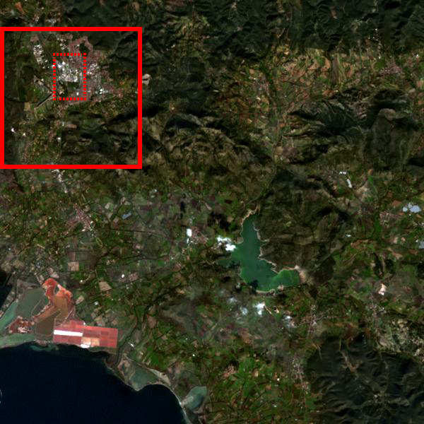
Ford County, Kansas, USA	Macuspana, Tabasco, MEX

Figure 2: Test set. HS (RGB bands) PRISMA test images. Red solid line-boxes indicate the tiles for FR tests. RR tests are carried out on the whole images. Dashed line-boxes spot the crops used for visualization purposes in the experimental part for both RR (green) and FR (red) tests.

TABLE V: PRISMA benchmark datasets: (A) Training, (B) Test.

Date Location Patches Land covers 27/06/20 Florence, Italy 14 Roofs, Streets, Crops, Hills, Water 13/08/20 Milan, Italy 13 Roofs, Streets, Crops 07/11/20 Bologna, Italy 13 Roofs, Streets, Crops, Hills 03/03/21 Kanpur, India 14 Roofs, Streets, Crops, Hills, Rivers 03/07/21 Willow Hill, Illinois 14 Streets, Crops, Hills, Rivers 19/06/22 Onaka, South Dakota 14 Crops, Swamps 03/07/22 Grosseto, Italy 14 Roofs, Streets, Crops, Hills 04/08/22 Bordeaux, France 14 Roofs, Streets, Crops 01/06/23 Dijon, France 13 Roofs, Streets, Crops 05/09/23 Ontario, Canada 14 Roofs, Streets, Crops, Hills, Rivers 09/09/23 London, UK 10 Roofs, Streets, Crops, Water 20/11/23 South Sardinia, Italy 16 Roofs, Streets, Crops, Hills, Water Total # of training patches 163 Total # of validation patches 24 (2/zone) Patch size for supervised training (RR): 192$\times$192 Patch size for unsupervised training (FR): 1152$\times$1152 Resolution ratio $R=6$ Bands $B=159/239$ Resolution: 30 m (RR) or 5 m (FR)

(A)

Date Location Land covers 05/09/22 Cagliari, Italy Roofs, Streets, Crops, Hills, Water 24/08/23 Udine, Italy Roofs, Streets, Crops, Water 08/09/23 Ford County, Kansas Streets, Crops 20/11/23 Macuspana, Tabasco Streets, Crops RR test image size: 600$\times$600 (from a 3600$\times$3600 real FR image) Real FR test image size: 1200$\times$1200 Resolution ratio $R=6$ Bands $B=159/239$ Resolution: 30 m (RR) or 5 m (FR)

(B)

IV-B Is this worth the effort?

We have already underlined what possible advantages HS pansharpening research can benefit from the use of a large and well-structured shared dataset. Here, we perform a very simple yet enlightening experiment in RR space to support our claims.

As noted above, in the absence of suitable datasets, a common practice for DL-based methods is to use a single image split into two non-overlapping parts for training and testing. To simulate this condition, we train our 5 supervised models, following the original experimental configurations, on a fraction (about 3/4) of the Udine image, listed in Tab.V(B), and test them on the remaining part, call these parts Udine/1 and Udine/2. Numerical results are reported in Tab. VI (only ERGAS for brevity). All five methods work quite well (on visual inspection) with very close ERGAS indicators, ranging from 1.7 to 2.1. Then, we train the same models on the proposed training set, see Tab. V(A), obtaining slightly worse results in all cases. As expected the statistical “alignment” between training and testing data offers some advantages. In fact, even if Udine/1 and Udine/2 are disjoint, they come from the same acquisition and share the same sensing geometry, daylight and atmosphere conditions, land cover, etc.

Things change completely when models are tested on a new image, Cagliari, again in Tab.V(B). The models trained on the proposed dataset exhibit a rather stable performance, with a slight average improvement concerning Udine/2. Neither Udine nor Cagliari contribute to the training set, so these results suggest that the latter can more easily pansharpened because of its simpler structure (see also Fig. 2). However, the models trained on Udine/1 suffer a catastrophic impairment, with ERGAS increasing by more than 80% on average. This is because their weights, over-fit to a small training set, are unable to generalize well to new data. In summary, this experiment, although limited in scope, confirms that the use of large, well-structured datasets improves generalization and prevents biases in experimental results.

TABLE VI: ERGAS scores with small/aligned vs large training datasets.

		Test image
method	Training	Udine/2	Cagliari
HyperPNN	Udine/1	1.8293	2.9550
	proposed dataset	2.1704	1.5802
HSpeNet	Udine/1	1.6823	3.6121
	proposed dataset	1.8948	1.2789
DIP-HyperKite	Udine/1	1.8905	3.3532
	proposed dataset	2.0212	2.4194
DHP-DARN	Udine/1	2.0758	4.6525
	proposed dataset	4.9047	2.0733
Hyper-DSNet	Udine/1	1.7190	2.5472
	proposed dataset	1.7748	1.2298

TABLE VII: Results at Reduced Resolution. Best, Top-5 and Worst-5 are in bold green, green and red. The average score is in the rightmost column.

Method		ERGAS						SAM						Q$2^{n}$
		Cagliari	Udine	Ford	Tabasco	Avg.		Cagliari	Udine	Ford	Tabasco	Avg.		Cagliari	Udine	Ford	Tabasco	Avg.
(Ideal)		0	0	0	0	0		0	0	0	0	0		1	1	1	1	1
EXP		1.7716	3.9587	1.6921	4.3650	2.9468		2.3073	4.6288	2.8528	6.3524	4.0353		0.5971	0.6453	0.7984	0.5935	0.6586
GSA		0.9389	2.4243	1.0008	2.8065	1.7926		1.8191	3.5730	2.2570	5.7455	3.3486		0.8739	0.8110	0.9201	0.7955	0.8501
BT-H		1.2784	3.4898	1.2462	3.1015	2.2790		2.3857	4.6059	2.5563	6.3532	3.9753		0.8180	0.7166	0.8941	0.7837	0.8031
BDSD-PC		1.1664	2.7627	1.2637	3.9316	2.2811		1.9439	5.0116	2.6646	7.8908	4.3777		0.8524	0.7904	0.9048	0.7144	0.8155
PRACS		1.1803	3.4688	1.2773	3.8578	2.4461		1.9742	4.2221	2.4571	6.2161	3.7174		0.8166	0.7144	0.8804	0.6778	0.7723
MTF-GLP-FS		0.9239	2.3660	0.9808	2.7356	1.7516		1.8123	3.4496	2.2297	5.7208	3.3031		0.8792	0.8218	0.9238	0.8026	0.8568
MTF-GLP-HPM		0.9292	4.0148	1.2231	3.0609	2.3070		1.8555	5.1824	2.6120	6.4104	4.0151		0.8833	0.6698	0.9000	0.7890	0.8105
MTF-GLP-HPM-R		0.9114	2.4661	0.9743	2.6967	1.7621		1.8121	3.3953	2.2124	6.0986	3.3796		0.8800	0.8134	0.9239	0.8023	0.8549
AWLP		1.1846	4.6926	1.3424	3.8592	2.7697		2.3323	7.9280	2.9252	7.7668	5.2381		0.8516	0.6290	0.8832	0.7496	0.7783
MF		1.1392	4.0155	1.5506	3.3944	2.5249		1.9213	4.5587	2.7173	6.2918	3.8723		0.8638	0.7263	0.8804	0.7807	0.8128
HySURE		1.4664	4.3476	2.0749	5.1119	3.2502		2.9264	6.6950	4.4153	9.0468	5.7709		0.7943	0.5761	0.7475	0.4951	0.6532
SR-D		1.8476	4.2618	1.8825	4.8011	3.1982		2.4242	6.1149	3.0551	7.9927	4.8967		0.5734	0.5846	0.7313	0.5440	0.6083
TV		1.2624	2.8864	1.3163	3.1771	2.1605		2.2212	4.0400	2.5705	5.6672	3.6247		0.8291	0.7833	0.8911	0.7692	0.8182
HyperPNN		1.2245	2.2237	1.1864	3.3557	1.9976		2.8925	4.3058	2.6461	7.0296	4.2185		0.8777	0.8539	0.9247	0.8229	0.8698
HSpeNet		1.0354	2.0527	1.0674	2.7964	1.7379		2.0644	3.2157	2.2838	5.8462	3.3525		0.8674	0.8588	0.9136	0.8245	0.8660
DHP-DARN		1.9137	4.4280	1.7389	4.7617	3.2106		3.4673	5.1740	3.3833	9.1288	5.2883		0.8489	0.8234	0.9190	0.7934	0.8462
DIP-HyperKite		1.3510	2.0206	1.0995	2.8092	1.8201		3.6543	5.8268	2.7089	9.1932	5.3458		0.8419	0.8497	0.9205	0.8201	0.8581
Hyper-DSNet		0.9725	1.8198	0.9820	2.4237	1.5495		1.9162	2.9638	2.1906	7.4854	3.6390		0.8833	0.8767	0.9303	0.8426	0.8832
R-PNN		0.9884	2.2256	1.0581	2.6704	1.7356		1.9720	3.5728	2.3860	5.6797	3.4026		0.8712	0.8225	0.9172	0.8112	0.8555
PCA-Z-PNN		1.0824	2.9062	1.5575	2.7813	2.0819		2.1124	4.6125	3.1154	5.5297	3.8425		0.8507	0.7798	0.8647	0.8116	0.8267

TABLE VIII: Results at Full Resolution. Best, Top-5 and Worst-5 are in bold green, green and red. The average score is in the rightmost column.

Method		$D_{\lambda}$						$D_{S}$						RQNR
		Cagliari	Udine	Ford	Tabasco	Avg.		Cagliari	Udine	Ford	Tabasco	Avg.		Cagliari	Udine	Ford	Tabasco	Avg.
(Ideal)		0.0000	0.0000	0.0000	0.0000	0.0000		0.0000	0.0000	0.0000	0.0000	0.0000		1.0000	1.0000	1.0000	1.0000	1.0000
EXP		0.0126	0.0077	0.0054	0.0106	0.0091		0.1306	0.1273	0.0704	0.1947	0.1308		0.8585	0.8660	0.9245	0.7967	0.8614
GSA		0.0227	0.0134	0.0078	0.0122	0.0140		0.0056	0.0074	0.0077	0.0184	0.0098		0.9718	0.9793	0.9846	0.9697	0.9763
BT-H		0.0633	0.0936	0.0195	0.0288	0.0513		0.0000	0.0000	0.0000	0.0002	0.0001		0.9367	0.9064	0.9805	0.9710	0.9487
BDSD-PC		0.0439	0.0256	0.0220	0.0487	0.0351		0.0024	0.0000	0.0001	0.0003	0.0007		0.9539	0.9744	0.9778	0.9510	0.9643
PRACS		0.0118	0.0155	0.0047	0.0088	0.0102		0.0083	0.0163	0.0114	0.0245	0.0151		0.9801	0.9684	0.9840	0.9670	0.9749
MTF-GLP-FS		0.0101	0.0054	0.0033	0.0065	0.0063		0.0214	0.0277	0.0174	0.0322	0.0247		0.9686	0.9671	0.9794	0.9616	0.9692
MTF-GLP-HPM		0.0147	0.0087	0.0067	0.0093	0.0098		0.0215	0.0284	0.0179	0.0389	0.0267		0.9641	0.9631	0.9756	0.9522	0.9637
MTF-GLP-HPM-R		0.0100	0.0057	0.0033	0.0074	0.0066		0.0217	0.0285	0.0176	0.0374	0.0263		0.9685	0.9660	0.9791	0.9554	0.9673
AWLP		0.0132	0.0097	0.0055	0.0092	0.0094		0.0251	0.0318	0.0206	0.0407	0.0295		0.9620	0.9588	0.9740	0.9504	0.9613
MF		0.0655	0.0392	0.0390	0.0331	0.0442		0.0389	0.0269	0.0250	0.0664	0.0393		0.8981	0.9349	0.9369	0.9027	0.9182
HySURE		0.1126	0.0618	0.0510	0.1158	0.0853		0.0022	0.0011	0.0016	0.0022	0.0018		0.8854	0.9372	0.9474	0.8823	0.9131
SR-D		0.0128	0.0087	0.0055	0.0115	0.0096		0.1316	0.1292	0.0720	0.1981	0.1327		0.8573	0.8632	0.9229	0.7927	0.8590
TV		0.0042	0.0028	0.0021	0.0036	0.0032		0.0586	0.0524	0.0358	0.0813	0.0570		0.9375	0.9449	0.9622	0.9154	0.9400
HyperPNN		0.0415	0.0139	0.0256	0.0248	0.0264		0.0036	0.0063	0.0040	0.0067	0.0051		0.9550	0.9799	0.9705	0.9687	0.9685
HSpeNet		0.0174	0.0084	0.0240	0.0154	0.0163		0.0101	0.0160	0.0141	0.0236	0.0159		0.9727	0.9758	0.9623	0.9614	0.9680
DHP-DARN		0.0832	0.0615	0.0467	0.0513	0.0607		0.0030	0.0053	0.0031	0.0130	0.0061		0.9141	0.9336	0.9503	0.9363	0.9336
DIP-HyperKite		0.0208	0.0125	0.0148	0.0146	0.0157		0.0042	0.0050	0.0043	0.0059	0.0048		0.9751	0.9826	0.9810	0.9796	0.9796
Hyper-DSNet		0.0119	0.0050	0.0082	0.0068	0.0080		0.0200	0.0246	0.0195	0.0346	0.0247		0.9683	0.9705	0.9725	0.9588	0.9675
R-PNN		0.0131	0.0091	0.0063	0.0074	0.0090		0.0168	0.0144	0.0129	0.0341	0.0195		0.9704	0.9766	0.9809	0.9587	0.9716
PCA-Z-PNN		0.0129	0.0041	0.0046	0.0080	0.0074		0.0152	0.0116	0.0088	0.0257	0.0153		0.9721	0.9844	0.9867	0.9665	0.9774

V Experimental results

This work aims to provide a comprehensive overview of the current HS pansharpening framework. This entails not only presenting and implementing classical and latest methods and evaluation metrics but also establishing guidelines for benchmarking and assessing these techniques, as well as highlighting open challenges and promising research directions in the field. With these goals in mind, it is crucial to set the basic characteristics of an ideal HS pansharpening algorithm which should:

• generalize across datasets;

• generalize across scales;

• preserve spectral features while raising spatial resolution;

• provide perceptually good visual results (for an ideal observer);

• be computationally efficient, especially at test time,

Properties (a)-(c) require reliable tools for numerical assessment, such as the SoTA indexes recalled in Section III, while (d) remains a subjective evaluation, but is no less important. Keeping the above properties in mind, we aim to point out the strengths and especially the limitations of current SoTA algorithms, which represent the main open challenges for future research. Note that we are not trying to establish some ranking among the techniques included in the benchmark, none of which is uniformly superior to the others. Instead, we would like to suggest a performance analysis methodology as a guideline for future research in the field.

Let us now delve into the numerical results summarized in Tab. VII and Tab. VIII for RR and FR datasets, respectively. For easier understanding, we have highlighted the 5 best and 5 worst performing techniques in green and red, respectively, with the best one emphasized in bold. Comments to the results are gathered and ordered according to the above list of quality features.

GT	GSA	BT-H	BDSD-PC	PRACS	MTF-GLP-FS	MTF-GLP-HPM	MTF-GLP-HPM-R	AWLP	MF
HySURE	SR-D	TV	HyperPNN	HSpeNet	DHP-DARN	DIP-HyperKite	Hyper-DSNet	R-PNN	PCA-Z-PNN
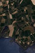
(a)
GT	GSA	BT-H	BDSD-PC	PRACS	MTF-GLP-FS	MTF-GLP-HPM	MTF-GLP-HPM-R	AWLP	MF
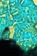
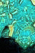
HySURE	SR-D	TV	HyperPNN	HSpeNet	DHP-DARN	DIP-HyperKite	Hyper-DSNet	R-PNN	PCA-Z-PNN
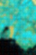
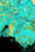
(b)

Figure 3: Pansharpening results (cropped: 120$\times$180) on Udine at reduced resolution. Target GT (visible range on top, NIR-SWIR at bottom) followed by all corresponding pansharpening results. Selected wavelenghts: $663,560,466$ nm (visible); $1943,1261,832$ nm (NIR-SWIR).

GT	GSA	BT-H	BDSD-PC	PRACS	MTF-GLP-FS	MTF-GLP-HPM	MTF-GLP-HPM-R	AWLP	MF
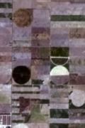
HySURE	SR-D	TV	HyperPNN	HSpeNet	DHP-DARN	DIP-HyperKite	Hyper-DSNet	R-PNN	PCA-Z-PNN
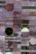
(a)
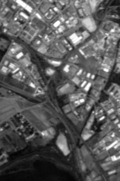
GT	GSA	BT-H	BDSD-PC	PRACS	MTF-GLP-FS	MTF-GLP-HPM	MTF-GLP-HPM-R	AWLP	MF
HySURE	SR-D	TV	HyperPNN	HSpeNet	DHP-DARN	DIP-HyperKite	Hyper-DSNet	R-PNN	PCA-Z-PNN
(b)

Figure 4: Pansharpening results (cropped: 120$\times$180) on Ford Country at reduced resolution. Target GT (visible range on top, NIR-SWIR at bottom) followed by all corresponding pansharpening results. Selected wavelenghts: $663,560,466$ nm (visible); $1943,1261,832$ nm (NIR-SWIR).

PAN	HS	GSA	BT-H	BDSD-PC	PRACS	MTF-GLP-FS
MTF-GLP-HPM	MTF-GLP-HPM-R	AWLP	MF	HySURE	SR-D	TV
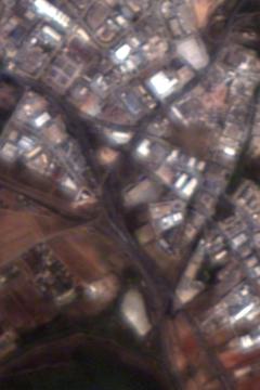
HyperPNN	HSpeNet	DHP-DARN	DIP- HyperKite	Hyper-DSNet	R-PNN	PCA-Z-PNN

Figure 5: Pansharpening results (cropped: 240$\times$360) on Cagliari at full resolution. PAN image followed by the HS component (bands in the visible range: $663,560,466$ nm; nearest-neighbor interpolation) and all corresponding pansharpening results.

PAN	HS	GSA	BT-H	BDSD-PC	PRACS	MTF-GLP-FS
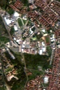
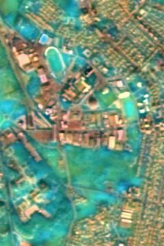
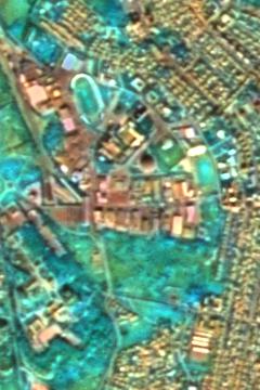
MTF-GLP-HPM	MTF-GLP-HPM-R	AWLP	MF	HySURE	SR-D	TV
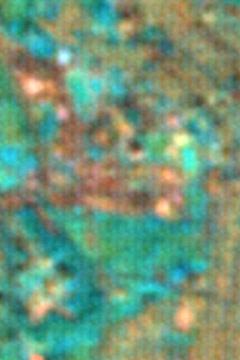
HyperPNN	HSpeNet	DHP-DARN	DIP- HyperKite	Hyper-DSNet	R-PNN	PCA-Z-PNN

Figure 6: Pansharpening results (cropped: 240$\times$360) on Cagliari at full resolution. PAN image followed by the HS component (bands in the NIR-SWIR: $1943,1261,832$ nm; nearest-neighbor interpolation) and all corresponding pansharpening results.

PAN	HS	GSA	BT-H	BDSD-PC	PRACS	MTF-GLP-FS
MTF-GLP-HPM	MTF-GLP-HPM-R	AWLP	MF	HySURE	SR-D	TV
HyperPNN	HSpeNet	DHP-DARN	DIP- HyperKite	Hyper-DSNet	R-PNN	PCA-Z-PNN

Figure 7: Pansharpening results (cropped: 240$\times$360) on Macuspana (Tabasco) at full resolution. PAN image followed by the HS component (bands in the visible range: $663,560,466$ nm; nearest-neighbor interpolation) and all corresponding pansharpening results.

PAN	HS	GSA	BT-H	BDSD-PC	PRACS	MTF-GLP-FS
MTF-GLP-HPM	MTF-GLP-HPM-R	AWLP	MF	HySURE	SR-D	TV
HyperPNN	HSpeNet	DHP-DARN	DIP- HyperKite	Hyper-DSNet	R-PNN	PCA-Z-PNN

Figure 8: Pansharpening results (cropped: 240$\times$360) on Macuspana (Tabasco) at full resolution. PAN image followed by the HS component (bands in the NIR-SWIR: $1943,1261,832$ nm; nearest-neighbor interpolation) and all corresponding pansharpening results.

Figure 9: Average running time [seconds] per 600$\times$600 image (RR test images) at inference. DL methods are run on GPU, and the remaining ones on CPU.

V-A Generalization across datasets

To assess a method’s ability to generalize across datasets, we fix the scale and index, e.g., ERGAS, reduced resolution, and analyze score variations across images. At reduced resolution (see Tab. VII) virtuous examples are MTF-GLP-FS and MTF-GLP-HPM-R, which exhibit high average scores for all three indexes, consistently across all test images. The same also holds for some DL-based methods, e.g., Hyper-DSNet, R-PNN, and others with worse average scores. Examples of methods with generalization issues at reduced resolution are MTF-GLP-HPM or PCA-Z-PNN. The former gets very good scores on Cagliari followed by bad ones on Udine. The latter performs well on Tabasco, but much worse on Ford.

Moving to the full resolution results in Tab. VIII, consistent behaviour is observed across the four test scenes for almost all methods on the spectral distortion index $D_{\lambda}$. However, while all reduced resolution indices can be considered alternative measures of overall quality, the full resolution indices $D_{\lambda}$ and $D_{S}$ each focus on a specific feature, i.e. spectral or spatial quality. Therefore, they are more likely to be uniform across images, following the characteristics of the method. Inconsistencies are more easily observed in the RQNR hybrid index since it results from the combination of $D_{\lambda}$ and $D_{S}$. This is the case, for example, of BT-H or BDSD-PC, which show opposite spectral and spatial behaviours resulting in unstable RQNR rankings.

V-B Generalization across scales

When moving from the reduced-resolution to the full-resolution domain, image statistics change considerably, even if the resolution downgrade is carried out carefully accounting for the sensor MTF characteristics. This is all the more true in our case, due to the rather large resolution ratio (six) of the PRISMA images. Overall, the cross-scale statistical mismatch is more important than the cross-scene mismatch and cross-scale generalization is not easily achieved.

To simplify the analysis of results, we consider only average scores, focusing, for each method, on the coherence between rankings registered at RR with those occurring at FR. The results of Tab. VII and Tab. VIII fully confirm that the methods generalize much better across different scenes than across scales. Some methods, like PRACS and PCA-Z-PNN, which struggle a bit at RR, seem to work well on FR data, while others, in particular some supervised DL-based method, suffer a performance hit when switching to FR tests. Examples of methods that tend to perform fairly well (but not top) at both scales are GSA, Hyper-DSNet and R-PNN. From these numbers, a picture emerges in which most methods seem to be optimized for just one scale, suffering on the other. In some cases, these results are the effect of an explicit design choice, as in the case of supervised DL methods, where training must be carried out in the RR domain. Given this apparent compromise, that is, working well only at one scale, one might wonder which one is preferable. On the one hand, the ultimate goal is to work well on FR data. On the other hand, at this scale, only consistency measures and not objective quality indicators can be observed. Eventually, the question remains open.

V-C Joint spectral-spatial quality

In fusing the PAN and HS components we aim to keep both the spatial detail of the former and the spectral richness of the latter. However, these goals are somewhat conflicting, and sometimes one property is obtained by sacrificing the other. To analyze this trade-off we can refer to the FR consistency indices, $D_{\lambda}$ and $D_{S}$, which evaluate spatial and spectral quality separately. Indeed, the FR results of Tab. VIII highlight several situations where this undesirable behaviour emerges clearly, with methods that show high scores on $D_{\lambda}$ but poor performance on $D_{S}$, or viceversa. The hybrid RQNR score, which weights the two indicators, can help evaluate the correct balance achieved by a method, with poor balance, signalled by a low RQNR, indicating ineffective fusion. Experimental results show that some recent DL-based methods, like DIP-HyperKite, R-PNN and PCA-Z-PNN, offer excellent RQNR scores. However, quite dated classical methods, like GSA and PRACS, are no less competitive. This confirms the observation already made in the introduction, that DL has yet to realize its full potential for HS pansharpening.

All this said we must raise a warning on our quality metrics. Spectral quality is relatively easy to assess, and Khan’s index $D_{\lambda}$ is quite robust and reliable. On the contrary, the assessment of spatial quality remains an open problem as testified by several recent works on the topic [86, 89]. Here, we decided to use $D_{S}$ in continuity with the prevalent literature and also with the recent HS pansharpening challenge [4]. However, like other metrics, $D_{S}$ has well-known shortcomings and failure cases. A good practice is to look first at the spectral quality, which can be reliably assessed through $D_{\lambda}$, and then move on to spatial quality, complementing numerical indicators with the visual inspection of sample results, which might spot undetected anomalies and incoherencies.

V-D Subjective visual quality

Since HS images comprise a very large number of spectral bands, examining them all individually would be unreasonable. On the other hand, these bands form a limited number of groups with high interband correlation. Therefore, as a reasonable compromise, we decided to show only six bands per sample image, grouped into two sets for false colour display, taken in the visible and NIR-SWIR ranges respectively. The “visible” bands correspond roughly to the red, green and blue wavelengths. The NIR-SWIR bands were selected such to have the minimum mutual correlation possible and be maximally representative of such a wide spectral range. Furthermore, to save space and show images at a reasonable resolution for visual inspection, only a small but significant crop per image was selected for display (spotted with dashed boxes in Fig. 2).

For the RR framework we selected crops from Udine (see Fig. 3) and Ford Country (see Fig. 4), showing results for visible bands on the top and NIR-SWIR bands on the bottom. On the top-left we show the ground truth (namely, the original HS), and then the pansharpening results for all methods. For both scenes, visual inspection seems to confirm the indications provided by the numerical results of Tab. VII. Without going into too much detail, it can be easily verified that images that appear too blurred or present spectral distortion correspond to methods ranked in the worst positions in Tab. VII. On the other hand, given the availability of the GT, numerical assessment is very reliable in this domain.

In the FR framework, visual inspection turns out to be much more informative. Here, lacking the GT, numerical results are less reliable as they only check consistency with the two input components, PAN and HS. Visual results are displayed in Figures 5-8 for crops taken from Cagliari and Tabasco, analyzed in the visible and NIR-SWIR ranges, respectively. In all cases, the original PAN and HS (the latter expanded to match sizes) are shown on the top left, followed by the output of all methods. The comparison with the original HS shows some significant spectral deviations (colours do not match) like for HyperPNN and DHP-DARN on Cagliari. In general, these problems were correctly predicted by the numerical indications of Tab. VIII). In most cases, the spectral quality is definitely good, both in the visible and NIR-SWIR ranges, confirming that spectral fidelity is not the main issue in HS pansharpening. The situation is more critical for spatial fidelity. By comparing results with the PAN, several problems emerge, concerning blurring or, on the opposite side, oversharpening. Some methods (PRACS, HySURE, SR-D, TV) produce systematic blurred outputs on both Cagliari and Tabasco and both in the visible and NIR-SWIR ranges. In some other cases, this is a spectrally selective phenomenon: for example, BDSD-PC blurs in the NIR-SWIR while AWLP blur in the visible range. Finally, in a few cases (HSpeNet, DIP-HyperKite) the blur is image-dependent, occurring only on Cagliari. In the opposite direction, some methods deliver over-sharpened output images, especially BT-H in the NIR-SWIR range.

These examples show that visual inspection plays a critical role in quality assessment, complementary to the role of numerical indicators. Actually, the disagreement with numerical results can shed light on the reliability of performance metrics. In particular, while $D_{\lambda}$ seems to be consistent with the visual results, $D_{S}$ shows some weakness as it does not always agree with the perceived spatial quality of the results. This is the case, for example, of BDSD-PC and HySURE ($D_{S}\approx 0$) whose results look somewhat blurred both in visible and NIR-SWIR ranges and present failures on vegetated areas as on the Tabasco image (Fig. 7). Similar inconsistencies can also be observed for other solutions, such as GSA and PRACS, having moderately good $D_{S}$ values.

V-E Computational Time

All experiments were carried out on the same server, an NVIDIA DGX Station A100, equipped with a 64-core AMD EPYC 7742 processor, 504 GB of DDR4 RAM, and four NVIDIA A100-SXM4 GPUs with 40 GB of GDDR5 memory each. The conventional CS, MRA, and MBO methods were run on the CPU, while the DL-based methods were run on a single GPU. The average run time for each method on the 600$\times$600 RR test images is reported in Fig. 9. The run times for the 4 times larger (1200$\times$1200) FR test images scale linearly with the size and hence are not reported. However, computational scalability depends on the available hardware, so we do not draw general conclusions about that. Some methods, both DL-based and not, have negligible run time, a quality to be considered in practical applications. Others are exceedingly slow, such as the CPU-based BDSD-PC and the GPU-based DHP-DARN. In general, all DL-based methods that try to adapt to the variability of input images pay a price in terms of computational complexity, DHP-DARN and DIP-HyperKite to estimate the deep image prior, and R-PNN and PCA-Z-PNN for the target-adaptation phase.

VI Conclusions

In this work, we proposed a benchmarking framework for HS pansharpening, aiming to provide the research community with an easy-to-use tool to develop and test new methods at a faster pace. Following a careful analysis of the SoTA, we have selected a series of reference methods, representative of the main and most promising approaches in the field. All methods have been re-implemented and are ready for use. In parallel, we designed a large dataset of real multiresolution PRISMA images (available on demand to the research community) to train and test all methods in a uniform environment and according to well-defined and stable protocols. To establish a solid starting point for future research, we tested all selected methods using established performance metrics. The analysis of the results allowed us to highlight the main problems of existing solutions and therefore the most promising research avenues.

In a way, we have taken a snapshot of the state of HS pansharpening research right now. However, this is not intended to freeze things: on the contrary, it aims to encourage further research, allow easier comparison of results, and provide a context for sharing tools, as well as ideas. In our vision, this framework is destined to expand with the help of interested researchers who can contribute new methods and data.

While claiming the merits of this initiative, we also see its limits. The set of methods selected is certainly not exhaustive and all choices are to a certain extent arbitrary. In particular, we could not reimplement some DL-based methods due to the lack of code and a sufficiently detailed description. The dataset itself, while representing a notable improvement over existing ones, is limited to a single sensor, thus preventing true generalization across sensors from being tested. Better performance parameters could probably be used to evaluate quality at full resolution. In summary, there is much room for contributions and improvements.

References

- [1] G. Vivone, L. Alparone, J. Chanussot, M. Dalla Mura, A. Garzelli, G. A. Licciardi, R. Restaino, and L. Wald, “A critical comparison among pansharpening algorithms,” IEEE Transactions on Geoscience and Remote Sensing, vol. 53, no. 5, pp. 2565–2586, 2014.
- [2] G. Vivone, M. Dalla Mura, A. Garzelli, R. Restaino, G. Scarpa, M. O. Ulfarsson, L. Alparone, and J. Chanussot, “A new benchmark based on recent advances in multispectral pansharpening: Revisiting pansharpening with classical and emerging pansharpening methods,” IEEE Geosci. Remote Sens. Mag., vol. 9, no. 1, pp. 53–81, 2021.
- [3] L.-j. Deng, G. Vivone, M. E. Paoletti, G. Scarpa, J. He, Y. Zhang, J. Chanussot, and A. Plaza, “Machine learning in pansharpening: A benchmark, from shallow to deep networks,” IEEE Geoscience and Remote Sensing Magazine, vol. 10, no. 3, pp. 279–315, 2022.
- [4] G. Vivone, A. Garzelli, Y. Xu, W. Liao, and J. Chanussot, “Panchromatic and hyperspectral image fusion: Outcome of the 2022 whispers hyperspectral pansharpening challenge,” IEEE J. Sel. Top. Appl. Earth Obs Remote Sens., vol. 16, pp. 166–179, 2023.
- [5] N. Audebert, B. Le Saux, and S. Lefevre, “Deep learning for classification of hyperspectral data: A comparative review,” IEEE Geoscience and Remote Sensing Magazine, vol. 7, no. 2, pp. 159–173, 2019.
- [6] S. Li, W. Song, L. Fang, Y. Chen, P. Ghamisi, and J. A. Benediktsson, “Deep learning for hyperspectral image classification: An overview,” IEEE Transactions on Geoscience and Remote Sensing, vol. 57, no. 9, pp. 6690–6709, 2019.
- [7] G. Zhang, S. Zhao, W. Li, Q. Du, Q. Ran, and R. Tao, “Htd-net: A deep convolutional neural network for target detection in hyperspectral imagery,” Remote Sensing, vol. 12, no. 9, 2020. [Online]. Available: https://www.mdpi.com/2072-4292/12/9/1489
- [8] L. Yan, M. Zhao, X. Wang, Y. Zhang, and J. Chen, “Object detection in hyperspectral images,” IEEE Signal Processing Letters, vol. 28, pp. 508–512, 2021.
- [9] C.-I. Chang, “Hyperspectral anomaly detection: A dual theory of hyperspectral target detection,” IEEE Transactions on Geoscience and Remote Sensing, vol. 60, pp. 1–20, 2022.
- [10] G. P. Petropoulos, K. Arvanitis, and N. Sigrimis, “Hyperion hyperspectral imagery analysis combined with machine learning classifiers for land use/cover mapping,” Expert Systems with Applications, vol. 39, no. 3, pp. 3800–3809, 2012. [Online]. Available: https://www.sciencedirect.com/science/article/pii/S0957417411014060
- [11] A. Vali, S. Comai, and M. Matteucci, “Deep learning for land use and land cover classification based on hyperspectral and multispectral earth observation data: A review,” Remote Sensing, vol. 12, no. 15, 2020. [Online]. Available: https://www.mdpi.com/2072-4292/12/15/2495
- [12] Y. Fu, G. Yang, Z. Li, H. Li, Z. Li, X. Xu, X. Song, Y. Zhang, D. Duan, C. Zhao, and L. Chen, “Progress of hyperspectral data processing and modelling for cereal crop nitrogen monitoring,” Computers and Electronics in Agriculture, vol. 172, p. 105321, 2020. [Online]. Available: https://www.sciencedirect.com/science/article/pii/S0168169919318253
- [13] N. Liu, P. A. Townsend, M. R. Naber, P. C. Bethke, W. B. Hills, and Y. Wang, “Hyperspectral imagery to monitor crop nutrient status within and across growing seasons,” Remote Sensing of Environment, vol. 255, p. 112303, 2021. [Online]. Available: https://www.sciencedirect.com/science/article/pii/S0034425721000213
- [14] M. Niroumand-Jadidi, F. Bovolo, and L. Bruzzone, “Water quality retrieval from prisma hyperspectral images: First experience in a turbid lake and comparison with sentinel-2,” Remote Sensing, vol. 12, no. 23, 2020. [Online]. Available: https://www.mdpi.com/2072-4292/12/23/3984
- [15] M. Pepe, L. Pompilio, B. Gioli, L. Busetto, and M. Boschetti, “Detection and classification of non-photosynthetic vegetation from prisma hyperspectral data in croplands,” Remote Sensing, vol. 12, no. 23, 2020. [Online]. Available: https://www.mdpi.com/2072-4292/12/23/3903
- [16] L. Capobianco, A. Garzelli, F. Nencini, L. Alparone, and S. Baronti, “Spatial enhancement of Hyperion hyperspectral data through ALI panchromatic image,” in 2007 IEEE International Geoscience and Remote Sensing Symposium, Jul. 2007, pp. 5158–5161.
- [17] Y. Zhang, S. De Backer, and P. Scheunders, “Noise-resistant wavelet-based bayesian fusion of multispectral and hyperspectral images,” IEEE Trans. Geosci. Remote Sens., vol. 47, no. 11, pp. 3834–3843, 2009.
- [18] M. Simoes, J. Bioucas-Dias, L. Almeida, and J. Chanussot, “A convex formulation for hyperspectral image superresolution via subspace-based regularization,” IEEE Trans. Geosci. Remote Sens., vol. 53, no. 6, pp. 3373–3388, 2015.
- [19] Q. Wei, N. Dobigeon, and J.-Y. Tourneret, “Bayesian fusion of multi-band images,” IEEE Journal of Selected Topics in Signal Processing, vol. 9, no. 6, pp. 1117–1127, 2015.
- [20] Q. Wei, J. Bioucas-Dias, N. Dobigeon, and J.-Y. Tourneret, “Hyperspectral and multispectral image fusion based on a sparse representation,” IEEE Transactions on Geoscience and Remote Sensing, vol. 53, no. 7, pp. 3658–3668, 2015.
- [21] O. Berné, A. Helens, P. Pilleri, and C. Joblin, “Non-negative matrix factorization pansharpening of hyperspectral data: An application to mid-infrared astronomy,” in 2010 2nd Workshop on Hyperspectral Image and Signal Processing: Evolution in Remote Sensing. IEEE, 2010, pp. 1–4.
- [22] M. Moeller, T. Wittman, and A. L. Bertozzi, “A variational approach to hyperspectral image fusion,” in Proc. SPIE, S. S. Shen and P. E. Lewis, Eds., vol. 7334. Orlando, Florida, USA: SPIE / International Society for Optical Engineering, May 2009, p. 73341E.
- [23] B. Huang, H. Song, H. Cui, J. Peng, and Z. Xu, “Spatial and spectral image fusion using sparse matrix factorization,” IEEE Transactions on Geoscience and Remote Sensing, vol. 52, no. 3, pp. 1693–1704, 2013.
- [24] R. Kawakami, Y. Matsushita, J. Wright, M. Ben-Ezra, Y.-W. Tai, and K. Ikeuchi, “High-resolution hyperspectral imaging via matrix factorization,” in CVPR 2011. IEEE, 2011, pp. 2329–2336.
- [25] G. Vivone, R. Restaino, G. Licciardi, M. Dalla Mura, and J. Chanussot, “Multiresolution analysis and component substitution techniques for hyperspectral pansharpening,” in Proc. IEEE IGARSS, 2014, pp. 2649–2652.
- [26] L. Loncan, L. De Almeida, J. Bioucas-Dias, X. Briottet, J. Chanussot, N. Dobigeon, S. Fabre, W. Liao, G. Licciardi, M. Simoes et al., “Hyperspectral pansharpening: A review,” IEEE Geosci. Remote Sens. Mag., vol. 3, no. 3, pp. 27–46, 2015.
- [27] J. Qu, Y. Li, and W. Dong, “Hyperspectral Pansharpening With Guided Filter,” IEEE Geosci. Remote Sensing Lett., vol. 14, no. 11, pp. 2152–2156, Nov. 2017.
- [28] P. Addesso, M. Dalla Mura, L. Condat, R. Restaino, G. Vivone, D. Picone, and J. Chanussot, “Collaborative total variation for hyperspectral pansharpening,” in 2017 IEEE International Geoscience and Remote Sensing Symposium, 2017, pp. 2597–2600.
- [29] Z. Huang, Q. Chen, Y. Shen, Q. Chen, and X. Liu, “An improved variational method for hyperspectral image pansharpening with the constraint of spectral difference minimization,” Int. Arch. Photogramm. Remote Sens. Spatial Inf. Sci., vol. XLII-2/W7, pp. 753–760, Sep. 2017.
- [30] W. Dong, J. Liang, and S. Xiao, “Saliency Analysis and Gaussian Mixture Model-Based Detail Extraction Algorithm for Hyperspectral Pansharpening,” IEEE Trans. Geosci. Remote Sensing, vol. 58, no. 8, pp. 5462–5476, Aug. 2020.
- [31] G. Masi, D. Cozzolino, L. Verdoliva, and G. Scarpa, “Pansharpening by convolutional neural networks,” Remote Sens., vol. 8, no. 7, p. 594, 2016. [Online]. Available: http://www.mdpi.com/2072-4292/8/7/594
- [32] J. Yang, X. Fu, Y. Hu, Y. Huang, X. Ding, and J. Paisley, “Pannet: A deep network architecture for pan-sharpening,” in ICCV, Oct. 2017.
- [33] M. Ciotola and G. Scarpa, “Fast full-resolution target-adaptive cnn-based pansharpening framework,” Remote Sens., vol. 15, no. 2, 2023. [Online]. Available: https://www.mdpi.com/2072-4292/15/2/319
- [34] L. He, J. Zhu, J. Li, A. Plaza, J. Chanussot, and B. Li, “HyperPNN: Hyperspectral Pansharpening via Spectrally Predictive Convolutional Neural Networks,” IEEE J. Sel. Top. Appl. Earth Obs Remote Sens., vol. 12, no. 8, pp. 3092–3100, Aug. 2019.
- [35] Y. Zheng, J. Li, Y. Li, J. Guo, X. Wu, and J. Chanussot, “Hyperspectral pansharpening using deep prior and dual attention residual network,” IEEE Trans. Geosci. Remote Sens., vol. 58, no. 11, pp. 8059–8076, 2020.
- [36] W. G. C. Bandara, J. M. J. Valanarasu, and V. M. Patel, “Hyperspectral pansharpening based on improved deep image prior and residual reconstruction,” IEEE Transactions on Geoscience and Remote Sensing, vol. 60, pp. 1–16, 2022.
- [37] G. Guarino, M. Ciotola, G. Vivone, and G. Scarpa, “Band-wise hyperspectral image pansharpening using cnn model propagation,” IEEE Transactions on Geoscience and Remote Sensing, vol. 62, pp. 1–18, 2024.
- [38] L. He, J. Zhu, J. Li, D. Meng, J. Chanussot, and A. Plaza, “Spectral-Fidelity Convolutional Neural Networks for Hyperspectral Pansharpening,” IEEE J. Sel. Top. Appl. Earth Observations Remote Sensing, vol. 13, pp. 5898–5914, 2020.
- [39] L. He, J. Zhu, J. Li, A. Plaza, J. Chanussot, and Z. Yu, “CNN-Based Hyperspectral Pansharpening With Arbitrary Resolution,” IEEE Trans. Geosci. Remote Sensing, vol. 60, pp. 1–21, 2022.
- [40] L. He, J. Xie, J. Li, A. Plaza, J. Chanussot, and J. Zhu, “Variable Subpixel Convolution Based Arbitrary-Resolution Hyperspectral Pansharpening,” IEEE Trans. Geosci. Remote Sensing, vol. 60, pp. 1–19, 2022.
- [41] P. Guan and E. Y. Lam, “Multistage Dual-Attention Guided Fusion Network for Hyperspectral Pansharpening,” IEEE Trans. Geosci. Remote Sensing, vol. 60, pp. 1–14, 2022.
- [42] X. Wu, J. Feng, R. Shang, X. Zhang, and L. Jiao, “Multiobjective Guided Divide-and-Conquer Network for Hyperspectral Pansharpening,” IEEE Trans. Geosci. Remote Sens., vol. 60, pp. 1–17, 2022.
- [43] J. Qu, Y. Shi, W. Xie, Y. Li, X. Wu, and Q. Du, “MSSL: Hyperspectral and Panchromatic Images Fusion via Multiresolution Spatial–Spectral Feature Learning Networks,” IEEE Trans. Geosci. Remote Sensing, vol. 60, pp. 1–13, 2022.
- [44] W. Dong, Y. Yang, J. Qu, W. Xie, and Y. Li, “Fusion of Hyperspectral and Panchromatic Images Using Generative Adversarial Network and Image Segmentation,” IEEE Trans. Geosci. Remote Sensing, vol. 60, pp. 1–13, 2022.
- [45] W. Dong, T. Zhang, J. Qu, S. Xiao, J. Liang, and Y. Li, “Laplacian Pyramid Dense Network for Hyperspectral Pansharpening,” IEEE Trans. Geosci. Remote Sensing, vol. 60, pp. 1–13, 2022.
- [46] S. Seo, J.-S. Choi, J. Lee, H.-H. Kim, D. Seo, J. Jeong, and M. Kim, “Upsnet: Unsupervised pan-sharpening network with registration learning between panchromatic and multi-spectral images,” IEEE Access, vol. 8, pp. 201 199–201 217, 2020.
- [47] M. Ciotola, S. Vitale, A. Mazza, G. Poggi, and G. Scarpa, “Pansharpening by convolutional neural networks in the full resolution framework,” IEEE Transactions on Geoscience and Remote Sensing, vol. 60, pp. 1–17, 2022.
- [48] M. Ciotola, G. Poggi, and G. Scarpa, “Unsupervised deep learning-based pansharpening with jointly enhanced spectral and spatial fidelity,” IEEE Trans. Geosci. Remote Sens., vol. 61, pp. 1–17, 2023.
- [49] J. Nie, Q. Xu, and J. Pan, “Unsupervised Hyperspectral Pansharpening by Ratio Estimation and Residual Attention Network,” IEEE Geosci. Remote Sensing Lett., vol. 19, pp. 1–5, 2022. [Online]. Available: https://ieeexplore.ieee.org/document/9703344/
- [50] G. Guarino, M. Ciotola, G. Vivone, G. Poggi, and G. Scarpa, “Pca-cnn hybrid approach for hyperspectral pansharpening,” IEEE Geosci. Remote Sens. Lett., vol. 20, pp. 1–5, 2023.
- [51] B. Aiazzi, S. Baronti, and M. Selva, “Improving component substitution pansharpening through multivariate regression of MS+Pan data,” IEEE Trans. Geosci. Remote Sens., vol. 45, no. 10, pp. 3230–3239, Oct. 2007.
- [52] S. Lolli, L. Alparone, A. Garzelli, and G. Vivone, “Haze correction for contrast-based multispectral pansharpening,” IEEE Geoscience and Remote Sensing Letters, vol. 14, no. 12, pp. 2255–2259, 2017.
- [53] G. Vivone, “Robust band-dependent spatial-detail approaches for panchromatic sharpening,” IEEE Transactions on Geoscience and Remote Sensing, vol. 57, no. 9, pp. 6421–6433, 2019.
- [54] J. Choi, K. Yu, and Y. Kim, “A new adaptive component-substitution-based satellite image fusion by using partial replacement,” IEEE Trans. Geosci. Remote Sens., vol. 49, no. 1, pp. 295–309, Jan 2011.
- [55] G. Vivone, R. Restaino, and J. Chanussot, “Full scale regression-based injection coefficients for panchromatic sharpening,” IEEE Transactions on Image Processing, vol. 27, no. 7, pp. 3418–3431, 2018.
- [56] L. Alparone, A. Garzelli, and G. Vivone, “Intersensor statistical matching for pansharpening: Theoretical issues and practical solutions,” IEEE Transactions on Geoscience and Remote Sensing, vol. 55, no. 8, pp. 4682–4695, 2017.
- [57] G. Vivone, R. Restaino, and J. Chanussot, “A regression-based high-pass modulation pansharpening approach,” IEEE Trans. Geosci. Remote Sens., vol. 56, no. 2, pp. 984–996, 2017.
- [58] X. Otazu, M. González-Audícana, O. Fors, and J. Núñez, “Introduction of sensor spectral response into image fusion methods. Application to wavelet-based methods,” IEEE Trans. Geosci. Remote Sens., vol. 43, no. 10, pp. 2376–2385, Oct. 2005.
- [59] R. Restaino, G. Vivone, M. Dalla Mura, and J. Chanussot, “Fusion of multispectral and panchromatic images based on morphological operators,” IEEE Trans. Image Process., vol. 25, no. 6, pp. 2882–2895, Jun. 2016.
- [60] M. R. Vicinanza, R. Restaino, G. Vivone, M. D. Mura, and J. Chanussot, “A pansharpening method based on the sparse representation of injected details,” IEEE Geosci. Remote Sens. Lett., vol. 12, no. 1, pp. 180–184, Jan 2015.
- [61] F. Palsson, J. R. Sveinsson, and M. O. Ulfarsson, “A new pansharpening algorithm based on total variation,” IEEE Geoscience and Remote Sensing Letters, vol. 11, no. 1, pp. 318–322, 2014.
- [62] Y.-W. Zhuo, T.-J. Zhang, J.-F. Hu, H.-X. Dou, T.-Z. Huang, and L.-J. Deng, “A deep-shallow fusion network with multidetail extractor and spectral attention for hyperspectral pansharpening,” IEEE Journal of Selected Topics in Applied Earth Observations and Remote Sensing, vol. 15, pp. 7539–7555, 2022.
- [63] T.-M. Tu, S.-C. Su, H.-C. Shyu, and P. S. Huang, “A new look at ihs-like image fusion methods,” Information Fusion, vol. 2, no. 3, pp. 177–186, 2001.
- [64] C. A. Laben and B. V. Brower, “Process for enhancing the spatial resolution of multispectral imagery using pan-sharpening,” 2000, U.S. Patent # 6,011,875.
- [65] B. Aiazzi, L. Alparone, S. Baronti, A. Garzelli, and M. Selva, “MTF-tailored multiscale fusion of high-resolution MS and Pan imagery,” Photogramm. Eng. Remote Sens., vol. 72, no. 5, pp. 591–596, May 2006.
- [66] A. R. Gillespie, A. B. Kahle, and R. E. Walker, “Color enhancement of highly correlated images. ii. channel ratio and “chromaticity” transformation techniques,” Remote Sensing of Environment, vol. 22, no. 3, pp. 343–365, 1987. [Online]. Available: https://www.sciencedirect.com/science/article/pii/0034425787900885
- [67] A. Garzelli, F. Nencini, and L. Capobianco, “Optimal MMSE pan sharpening of very high resolution multispectral images,” IEEE Trans. Geosci. Remote Sens., vol. 46, no. 1, pp. 228–236, Jan 2008.
- [68] S. Baronti, B. Aiazzi, M. Selva, A. Garzelli, and L. Alparone, “A theoretical analysis of the effects of aliasing and misregistration on pansharpened imagery,” IEEE Journal of Selected Topics in Signal Processing, vol. 5, no. 3, pp. 446–453, 2011.
- [69] C. Thomas, T. Ranchin, L. Wald, and J. Chanussot, “Synthesis of multispectral images to high spatial resolution: A critical review of fusion methods based on remote sensing physics,” IEEE Transactions on Geoscience and Remote Sensing, vol. 46, no. 5, pp. 1301–1312, 2008.
- [70] G. Vivone, R. Restaino, M. Dalla Mura, G. Licciardi, and J. Chanussot, “Contrast and error-based fusion schemes for multispectral image pansharpening,” IEEE Geoscience and Remote Sensing Letters, vol. 11, no. 5, pp. 930–934, 2013.
- [71] Q. Wei, N. Dobigeon, and J.-Y. Tourneret, “Fast fusion of multi-band images based on solving a sylvester equation,” IEEE Transactions on Image Processing, vol. 24, no. 11, pp. 4109–4121, 2015.
- [72] J. M. Bioucas-Dias, A. Plaza, N. Dobigeon, M. Parente, Q. Du, P. Gader, and J. Chanussot, “Hyperspectral unmixing overview: Geometrical, statistical, and sparse regression-based approaches,” IEEE Journal of Selected Topics in Applied Earth Observations and Remote Sensing, vol. 5, no. 2, pp. 354–379, 2012.
- [73] M. Farrell and R. Mersereau, “On the impact of pca dimension reduction for hyperspectral detection of difficult targets,” IEEE Geoscience and Remote Sensing Letters, vol. 2, no. 2, pp. 192–195, 2005.
- [74] J. Nascimento and J. Dias, “Vertex component analysis: a fast algorithm to unmix hyperspectral data,” IEEE Transactions on Geoscience and Remote Sensing, vol. 43, no. 4, pp. 898–910, 2005.
- [75] R. Molina, A. Katsaggelos, and J. Mateos, “Bayesian and regularization methods for hyperparameter estimation in image restoration,” IEEE Transactions on Image Processing, vol. 8, no. 2, pp. 231–246, 1999.
- [76] R. Hardie, M. Eismann, and G. Wilson, “MAP estimation for hyperspectral image resolution enhancement using an auxiliary sensor,” IEEE Transactions on Image Processing, vol. 13, no. 9, pp. 1174–1184, 2004.
- [77] R. Molina, M. Vega, J. Mateos, and A. K. Katsaggelos, “Variational posterior distribution approximation in bayesian super resolution reconstruction of multispectral images,” Applied and Computational Harmonic Analysis, vol. 24, no. 2, pp. 251–267, 2008, special Issue on Mathematical Imaging – Part II.
- [78] A. K. Gupta and D. K. Nagar, Matrix variate distributions, ser. Chapman & Hall/CRC monographs and surveys in pure and applied mathematics. Chapman & Hall/CRC, 2000, vol. 104.
- [79] L. Wald, T. Ranchin, and M. Mangolini, “Fusion of satellite images of different spatial resolutions: Assessing the quality of resulting images,” Photog. Eng. and Remote Sens., vol. 63, no. 6, pp. 691–699, 1997.
- [80] R. H. Yuhas, A. F. H. Goetz, and J. W. Boardman, “Discrimination among semi-arid landscape endmembers using the Spectral Angle Mapper (SAM) algorithm,” in Proc. Summaries 3rd Annu. JPL Airborne Geosci. Workshop, 1992, pp. 147–149.
- [81] V. Lempitsky, A. Vedaldi, and D. Ulyanov, “Deep image prior,” in 2018 IEEE/CVF Conference on Computer Vision and Pattern Recognition, 2018, pp. 9446–9454.
- [82] O. Ronneberger, P. Fischer, and T. Brox, “U-net: Convolutional networks for biomedical image segmentation,” in Medical Image Computing and Computer-Assisted Intervention – MICCAI 2015, N. Navab, J. Hornegger, W. M. Wells, and A. F. Frangi, Eds. Cham: Springer International Publishing, 2015, pp. 234–241.
- [83] S. Luo, S. Zhou, Y. Feng, and J. Xie, “Pansharpening via unsupervised convolutional neural networks,” IEEE Journal of Selected Topics in Applied Earth Observations and Remote Sensing, vol. 13, pp. 4295–4310, 2020.
- [84] M. Ciotola, M. Ragosta, G. Poggi, and G. Scarpa, “A full-resolution training framework for sentinel-2 image fusion,” in 2021 IEEE International Geoscience and Remote Sensing Symposium IGARSS, 2021, pp. 1260–1263.
- [85] G. Scarpa, S. Vitale, and D. Cozzolino, “Target-adaptive cnn-based pansharpening,” IEEE Trans. Geosci. Remote Sens., vol. 56, no. 9, pp. 5443–5457, 2018.
- [86] G. Scarpa and M. Ciotola, “Full-resolution quality assessment for pansharpening,” Remote Sens., vol. 14, no. 8, 2022. [Online]. Available: https://www.mdpi.com/2072-4292/14/8/1808
- [87] G. Vivone, M. Dalla Mura, A. Garzelli, and F. Pacifici, “A benchmarking protocol for pansharpening: Dataset, preprocessing, and quality assessment,” IEEE Journal of Selected Topics in Applied Earth Observations and Remote Sensing, vol. 14, pp. 6102–6118, 2021.
- [88] L. Alparone, B. Aiazzi, S. Baronti, A. Garzelli, F. Nencini, and M. Selva, “Multispectral and panchromatic data fusion assessment without reference,” Photog. Eng. and Remote Sens., vol. 74, no. 2, pp. 193–200, 2008.
- [89] A. Arienzo, G. Vivone, A. Garzelli, L. Alparone, and J. Chanussot, “Full resolution quality assessment of pansharpening: Theoretical and hands-on approaches,” IEEE Geosci. Remote Sens. Mag., 2022.
- [90] L. Wald, Data Fusion: Definitions and Architectures — Fusion of images of different spatial resolutions. Paris, France: Les Presses de l’École des Mines, 2002.
- [91] A. Garzelli and F. Nencini, “Hypercomplex quality assessment of multi/hyperspectral images,” IEEE Trans. Geosci. Remote Sens., vol. 6, no. 4, pp. 662–665, Oct. 2009.
- [92] Z. Wang and A. C. Bovik, “A universal image quality index,” IEEE Sig. Proc. Lett., vol. 9, no. 3, pp. 81–84, 2002.
- [93] M. M. Khan, L. Alparone, and J. Chanussot, “Pansharpening quality assessment using the modulation transfer functions of instruments,” IEEE transactions on geoscience and remote sensing, vol. 47, no. 11, pp. 3880–3891, 2009.
- [94] L. Alparone, A. Garzelli, and G. Vivone, “Spatial consistency for full-scale assessment of pansharpening,” in IGARSS 2018-2018 IEEE International Geoscience and Remote Sensing Symposium. IEEE, 2018, pp. 5132–5134.
- [95] G. Vivone, A. Garzelli, Y. Xu, W. Liao, and J. Chanussot, “Panchromatic and hyperspectral image fusion: outcome of the 2022 whispers hyperspectral pansharpening challenge,” IEEE J. Sel. Top. Appl. Earth Obs Remote Sens., vol. 16, pp. 166–179, 2022.
- [96] R. Carla, L. Santurri, B. Aiazzi, and S. Baronti, “Full-scale assessment of pansharpening through polynomial fitting of multiscale measurements,” IEEE Transactions on Geoscience and Remote Sensing, vol. 53, no. 12, pp. 6344–6355, 2015.
- [97] G. Vivone, R. Restaino, and J. Chanussot, “A Bayesian procedure for full-resolution quality assessment of pansharpened products,” IEEE Transactions on Geoscience and Remote Sensing, vol. 56, no. 8, pp. 4820–4834, 2018.
- [98] O. A. Agudelo-Medina, H. D. Benitez-Restrepo, G. Vivone, and A. Bovik, “Perceptual quality assessment of pan-sharpened images,” Remote Sensing, vol. 11, no. 7, p. 877, 2019.