Multi-level Reliable Guidance for Unpaired Multi-view Clustering

Abstract

In this paper, we address the challenging problem of unpaired multi-view clustering (UMC), aiming to perform effective joint clustering using unpaired observed samples across multiple views. Commonly, traditional incomplete multi-view clustering (IMC) methods often depend on paired samples to capture complementary information between views. However, the strategy becomes impractical in UMC due to the absence of paired samples. Although some researchers have attempted to tackle the issue by preserving consistent cluster structures across views, they frequently neglect the confidence of these cluster structures, especially for boundary samples and uncertain cluster structures during the initial training. Therefore, we propose a method called Multi-level Reliable Guidance for UMC (MRG-UMC), which leverages multi-level clustering to aid in learning a trustworthy cluster structure across inner-view, cross-view, and common-view, respectively. Specifically, within each view, multi-level clustering fosters a trustworthy cluster structure across different levels and reduces clustering error. In cross-view learning, reliable view guidance enhances the confidence of the cluster structures in other views. Similarly, within the multi-level framework, the incorporation of a common view aids in aligning different views, thereby reducing the clustering error and uncertainty of cluster structure. Finally, as evidenced by extensive experiments, our method for UMC demonstrates significant efficiency improvements compared to 20 state-of-the-art methods.

I Introduction

Data often exhibit diverse characteristics and representations, referred to as multi-view data [1, 2, 3, 4]. In the real world, some instances lack data in one view or more, resulting in incomplete multi-view data [5, 6]. For example, in a news story dataset, articles are gathered from various online platforms, but not all news is reported on each platform. Similarly, in an image dataset, some images may lack certain visual or textual features. Unfortunately, there exists an extreme yet realistic scenario where no paired observed samples exist between views [7, 8], rendering the multi-view data as unpaired multi-view data. For example, in multi-camera surveillance systems, individual cameras may operate intermittently due to energy-saving or maintenance, resulting in unpaired multi-view data [7, 8, 9]. Additionally, in a video, if we view a visible video and accompanying narrator text as separate views, the description may become disjointed from the visual content due to delays, resulting in the occurrence of unpaired multi-view data [10].

Clustering [11] serves as a potent technique for uncovering inherent patterns within data, segmenting samples into distinct clusters autonomously without supervised information. For the three types of datasets mentioned above, three downstream clustering tasks—multi-view clustering (MC), incomplete multi-view clustering (IMC), and unpaired multi-view clustering (UMC)—naturally emerge. Specifically, UMC is more challenging than MC and IMC due to the absence of paired samples. In MC and IMC, researchers leverage the complete observed samples to construct relationships between views. However, in UMC, it is difficult to construct these relationships due to the absence of paired samples. Furthermore, the lack of supervised information makes obtaining a certain cluster assignment challenging.

Recently, some methods have leveraged consistent cluster structures to connect different views in UMC. For example, Yang et al . [7] leverage covariance matrix to align different views. Xin et al . [8] use the inner-view and cross-view contrastive learning to learn the consistent cluster structure. Besides, Xin et al . [9] leverage the cluster structures of reliable views to guide the other views. However, they often overlook the confidence of these cluster structures, which may affect their effectiveness in handling boundary samples and initially uncertain cluster structures. Therefore, we aim to enhance the confidence of cluster structures across multiple views.

To solve this issue, we consider multi-level clustering to enhance the quality of cluster structures step by step. Typically, classification is relatively easy with a small number of classes, whereas it becomes increasingly challenging as the number of classes increases. For instance, in a dataset with five categories (flowers, trees, chickens, dogs, horses), the accuracy of binary classification (animals vs. plants) is expected to be notably higher than that of multi-class classification (five categories). Therefore, coarse-grained classification generally yields better results compared to fine-grained classification [12]. Similarly, coarse-grained clustering exhibits fewer clustering errors than fine-grained clustering. As depicted in Fig. 1, the smaller the number of clusters, the more accurately a cluster can roughly categorize samples. Besides, clustering with just single-level, cluster errors can spread across the entire category, affecting final results. Hence, instead of directly assigning pseudo labels, multi-level clustering provides multi-level softer results, effectively mitigating the cluster errors from boundary samples and initially uncertain cluster structures. Naturally, we create a rough cluster set aiding in dynamically forming multi-level clustering to ‘roughly categorize’ samples (shown in Fig. 1). Subsequently, multi-level clustering is integrated with consistent cluster structures to form multi-level reliable cluster structures. It is worth noting that multi-layer clustering is different from hierarchical clustering. Hierarchical clustering is a nested structure where the results of the next clustering are based on the previous ones. In contrast, in multi-layer clustering, the results on each layer are performed independently of the previous layer. Therefore, the purpose of multi-layer clustering in this paper is to preserve sample pairs with stable relationships across different layers.

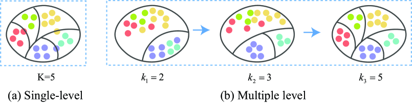
Figure 1: The example of single-level clustering and multi-level clustering. In the single-level scenario, boundary samples occur when $K=5$. In multi-level clustering, the clusters merge with a rough cluster set $Cs=\{k_{1},k_{2},k_{3}\}$. The number of boundary samples at $k_{3}$ is reduced with the help of $k_{1}$ and $k_{2}$, thereby decreasing clustering errors and enhancing accuracy.

Specifically, we improve the confidence of the consistent cluster structure from three aspects: 1) inner-view multi-level clustering. To ensure a consistent cluster structure within a view, we introduce inner-view contrastive learning within the multi-level clustering. This constraint is designed to preserve the stability of cluster structure relationships across different levels. Consequently, more trustworthy sample relationships are established, leading to fewer cluster errors. 2) Cross-view multi-level guidance. The reliability of views varies based on their clustering performance. On each level, with the assistance of reliable view guidance, the views with less reliable cluster structures are enhanced, thereby establishing a more trustworthy cluster structure, similar to that of the reliable views. 3) Common-view multi-level guidance. The sample distributions across views vary greatly, making it challenging to align them directly. On each level, the common view as an auxiliary aids in aligning other views, thereby reducing learning difficulty and improving consistency in cluster structures. Therefore, to enhance the confidence of views, we propose a novel method, Multi-level Reliable Guidance for UMC (MRG-UMC), which aims to eliminate cluster errors and learn a consistent reliable cluster structure. The main contributions of MRG-UMC can be summered as follows:

• We propose a multi-level guidance strategy instead of a single-level approach to enhance the confidence of cluster structures, which is commonly overlooked in most methods.

• We propose a novel method, MRG-UMC, under multi-level clustering, which comprises three modules: an inner-view multi-level clustering module, a cross-view multi-level guidance module, and a common-view multi-level guidance module. This approach helps alleviate clustering errors caused by boundary samples and initial uncertain cluster structures, thereby forming a reliable cluster structure across views.

• Extensive experiments on five multi-view benchmark datasets show excellent performance compared with the sixteen state-of-the-art methods.

II Related Work

II-A Incomplete multi-view clustering

In real-world scenarios, samples may be missing in one or more views due to various internal or external factors, resulting in incomplete multi-view data. To address this challenge in clustering tasks, researchers have extensively explored methods such as spectral approaches, subspace learning, and graph learning [7, 8]. In spectral approaches, Wen et al . [13] introduced a tensor spectral clustering method to recover missing views. Besides, they utilize latent information from absent views and capture intra-view data relationships often overlooked in other methods. Zhang et al . [14] restored latent connections between observed and unobserved samples, enhancing the robustness of subspace clustering through high-level correlations. It is the first attempt to formulate incomplete multi-view kernel subspace clustering from unified and tensorized perspectives. Wang et al . [15] used multiple kernel-based anchor graphs to tackle IMC. which adeptly captures both intra-view and inter-view nonlinear relationships by fusing multiple complete anchor graphs across views. For the time-consuming of recovering the original data, Zhang et al . [16] devised an approach that integrates spectral embedding completion and discrete cluster indicator learning into a unified step, providing a solution to this issue.

For graph learning, Li et al . [17] proposed the Joint Partition and Graph learning method, comprising two key components: unified partition space learning for noise robustness enhancement and consensus graph learning for uncovering data structures. To explore the complex relationship between samples and latent representations, Zhu et al . [18] proposed a neighborhood constraint and a view-existence constraint for the first time. Besides, in cases of arbitrary missing views, He et al . [19] proposed Structured Anchor-inferred Graph Learning. They replaced a fixed distance-based weighting matrix with a structural anchor-based similarity learning model, creating a trainable asymmetric intra-view similarity matrix. Furthermore, to learn an overall optimal clustering result, Xia et al . [20] proposed a Kernelized Graph-based IMC algorithm, which optimizes the downstream sub-tasks in a mutual reinforcement manner.

For subspace learning approaches, Yin et al . [21] devised a method for incomplete multi-view subspace learning, which enhances performance by simultaneously addressing feature selection and similarity preservation within and across views. To fully leverage observed samples, Yang et al . [22] employed a sparse and low-rank matrix to model correlations among samples within each view for imputing missing samples. They also enforce similar subspace representations to explore relationships between samples across different views, aiding clustering tasks. Thanks to the coefficient matrix, the self-representation method accurately captures sample relationships. Liu et al . [23] introduced a tailored self-representation subspace clustering algorithm for IMC, which integrates missing sample completion and self-representation learning into a cyclical process. Yang et al . [24] integrated the intrinsic consistency and extrinsic complementary information for prediction and cluster simultaneously. Li et al . [25] proposed a unified sparse subspace learning framework that integrates inter-view and intra-view affinities to generate the unified clustering assignment using a sparse anchor graph. However, obtaining matched samples across all views can be challenging in real-world scenarios.

II-B Unpaired multi-view clustering

UMC is an extreme scenario within IMC, where samples are solely observed in one view. This renders UMC more challenging compared to IMC [7, 8]. Numerous researchers have leveraged weak supervision information to establish correlations between views. For example, Qian et al . [26] and Houthuys et al . [27] integrated must-link and cannot-link constraints to build correlations across views in their studies. However, these approaches may prove ineffective without paired samples or supervised information.

For methods dealing with partially paired samples, Huang et al . [28] proposed Partially View-Aligned Clustering, which utilizes the ‘aligned’ data to learn a common space across different views and employs a neural network to establish category-level correspondence for unaligned data. Yang et al . [29] proposed Multiview Contrastive Learning with Noise-Robust Loss, which simultaneously learns representation and aligns data using a noise-robust contrastive loss. Furthermore, addressing both the partially view-unaligned and sample-missing problem, Yang et al . [30] introduced a more robust Multi-View Clustering method to directly re-align and recover samples from other views. Besides, Wang et al . [31] introduced the Cross-View Graph Contrastive Learning Network, which integrates multi-view information to align data and learn latent representations. Jin et al . [32] proposed a novel approach departing from traditional contrastive-based methods. They use pair-observed data alignment as ‘proxy supervised signals’ to guide instance-to-instance correspondences across views. Additionally, they introduce a prototype alignment module to rectify shifted prototypes in IMVC. However, these methods require some paired samples to establish relationships between views.

For methods dealing with unpaired data, Yang et al . [33] proposed the Noise-aware Image Captioning (NIC) method to make the most of trustworthy information in text with mismatched words. Specifically, NIC identified and explored mismatched words to reduce errors by assessing the reliability of word-label relationships based on inter-modal representativeness and intra-modal informativeness. Additionally, Yang et al . [7] introduced Iterative Multiview Subspace Learning for UMC to learn consistent subspace representations. Expanding on this work, they introduced another two methods to solve multi-view alignment and achieve end-to-end results, respectively. Besides, Xin et al . [8] proposed selective contrastive learning for UMC, leveraging inner-view and inter-view selective contrastive learning modules to improve cluster structure consistency. However, the method focuses on view consistency, overlooking their potential complementary. Therefore, considering the differences in cluster structures across views, Xin et al . [9] leveraged the cluster structures of reliable views to guide those of the other views, thereby improving the overall clustering performance. Although these methods explore consistent cluster structures among views, they commonly overlook the confidence of these cluster structures.

II-C Dempster-Shafer evidence theory in multi-view learning

There have been several studies exploring confidence with Dempster-Shafer evidence theory. The theory was first proposed by Dempster and Shafer to deal with uncertainty based on belief functions [34, 35, 36]. Now, it has been developed a general framework. Recently, Han et al . [37] introduced multi-modal dynamics to enhance the reliability of fusion methods using evidence theory, dynamically evaluating feature-level and modality-level informativeness for dependable integration across diverse samples. Geng et al . [38] utilize uncertainty to weigh each view of individual samples based on data quality, maximizing the use of high-quality samples while minimizing the influence of noisy ones. Additionally, Han et al . [39] introduced a trusted multi-view classification method, dynamically integrating diverse views using the Dirichlet distribution for class probabilities and Dempster-Shafer theory for integration. Furthermore, they provide additional theoretical analysis to validate its effectiveness. Furthermore, for unreliable predictions in long-tailed classification, Li et al . [40] introduced the trustworthy long-tailed classification method, which integrates classification and uncertainty estimation within a multi-expert framework, calculating evidence-based uncertainty and evidence for each expert, and merging these metrics using the Dempster-Shafer Evidence Theory.

II-D Multi-level feature learning for multi-view clustering

For the method with multi-level feature learning, Xu et al . [41] proposed a method of multi-level feature learning with low-level features, high-level features, and semantic features to weaken the conflict between learning consistent common semantics and inconsistent view-private information. To develop a robust network, Yang et al . [42] introduced the Cascade Deep Multi-Modal network structure with a cascade architecture, which maximizes correlations between layers sharing similar characteristics. Furthermore, to address the next-item recommendation issue, Yang et al . [43] considered both user intentions and preferences, capturing users’ dynamic information in hierarchical representations. In response to existing methods neglecting redundant information between views, Cui et al . [44] proposed a novel multi-view clustering framework based on information theory. The method employs variational analysis to generate consistent information and introduces a sufficient representation of lower bound to enhance consistency. Besides, to tackle the issue of semantic consistency oversight in most methods, Zhou et al . [45] introduced a multi-level consistency collaborative learning framework, which learns cluster assignments of multiple views in the feature space and aligns semantic labels of different views through contrastive learning. Wang et al . [46] proposed multi-level representation learning contrastive and adversarial learning to achieve a balance between data restoration and clustering, while also capturing the consistency of representations across different views.

Although these methods leverage multi-level representation or features to learn consistent information, they fail to consider the consistent cluster structure among different levels, which is the main distinction between these methods and our approach.

III Methodology

III-A Notations and Architecture

Notations. For the unpaired multi-view dataset $\{\boldsymbol{X}^{v}\}_{v=1}^{V}$, it has $V$ views. The feature dimension on each view is denoted as $d^{v}$, where $v$ ranges from 1 to $V$. For the $v$-th view, the sample number is $n^{v}$. Therefore, for the no paired samples that exist in UMC, the total sample number of the unpaired multi-view dataset with $V$ views is $N$, where $N=\sum_{v=1}^{V}n^{v}$. Specifically, an autoencoder consists of an encoder and a decoder, which are denoted as $F^{v}$ and $G^{v}$ respectively, in the $v$-th view. For the $v$-th view data $\boldsymbol{X}^{v}$, we fed them into a specific encoder $F^{v}$ to learn the latent representation $\boldsymbol{Z}^{v}$, i.e., $\boldsymbol{Z}^{v}=F(\boldsymbol{X}^{v})$. In the inner-view multi-level clustering module, for sample $\boldsymbol{z}_{i}^{v}$, true positive pairs similarity set $tp_{in}(\boldsymbol{z}_{i}^{v})$ and true negative pairs similarity set $tn_{in}(\boldsymbol{z}_{i}^{v})$ are take into consideration in the contrastive learning. In the cross-view multi-level guidance module, reliable views are those with a better cluster structure than the current view, which is selected based on silhouette coefficients $sils^{v}$. The index set of reliable views is denoted as $\mathcal{C}$. Then two approximate probability distributions $P^{v}$ and $Q^{r}$ are utilized in the KL divergence to align the $v$-th and $r$-th views. In the common-view multi-level guidance module, a matrix of cluster pairing relationships $\boldsymbol{A}$ between views is established by the Hungarian Algorithm. Then, the similarity sets $pos_{cro}(\boldsymbol{z}_{i}^{v})$ and $neg_{cro}(\boldsymbol{z}_{i}^{v})$ for the positive and negative pairs of $\boldsymbol{z}_{i}^{v}$ are constructed. For clarity, we include the main symbols and their definitions in TABLE I.

TABLE I: Main notations used in this paper.

Notations	Descriptions
$V;N;K$	The number of views, samples, and actual clusters
$n^{v};d^{v}$	The number and dimension of the $v$-th view observations
$D$	The dimension of latent representation
$\boldsymbol{X}^{v}\in{\mathbb{R}^{n^{v}\times d^{v}}}$	Sample of the $v$-th view observations
$\hat{\boldsymbol{X}}^{v}\in{\mathbb{R}^{n^{v}\times d^{v}}}$	The reconstruction of the $v$-th view observations
$\boldsymbol{Z}^{v}\in{\mathbb{R}^{n^{v}\times D}}$	Subspace representation of the $v$-th view observations
$\boldsymbol{Z}^{*}\in{\mathbb{R}^{N\times D}}$	Common subspace representation $\boldsymbol{Z}^{*}=[\boldsymbol{Z}^{1};\ldots;\boldsymbol{Z}^{V}]$
$\boldsymbol{C}^{v}\in{\mathbb{R}^{K\times D}}$	Clustering centroids of latent representation of $v$-th view
$\boldsymbol{C}^{*}\in{\mathbb{R}^{K\times D}}$	Clustering centroids of common representation
$\boldsymbol{A}^{v}\in\{0,1\}^{K\times K}$	The pairing relationship between $\boldsymbol{C}^{*}$ and $\boldsymbol{C}^{v}$
$\boldsymbol{s}_{ij}^{v}$	The similarities of $\boldsymbol{z}_{i}^{v}$ and $\boldsymbol{z}_{j}^{v}$
$sils^{v}$	The silhouette coefficient value for $v$-th view
$tp_{in}(\boldsymbol{z}_{i}^{v})$	The true positive pairs similarity set of $\boldsymbol{z}_{i}^{v}$
$tn_{in}(\boldsymbol{z}_{i}^{v})$	The true negative pairs similarity set of $\boldsymbol{z}_{i}^{v}$
$pos_{cro}(\boldsymbol{z}_{i}^{v})$	The positive pairs similarity set of $\boldsymbol{z}_{i}^{v}$
$neg_{cro}(\boldsymbol{z}_{i}^{v})$	The negative pairs similarity set of $\boldsymbol{z}_{i}^{v}$
$c({\boldsymbol{z}^{v,k}_{i}}),nc({\boldsymbol{z}^{v,k}_{i}})$	The sample sets with same and different clusters as
	$\boldsymbol{z}^{v}_{i}$ with $k$ clusters, respectively
$\mathcal{C}$	The set of indices for reliable views
$P^{v}$	The probability distributions of the $v$-th view
$Q^{r}$	The probability distributions of the $r$-th reliable view
$F^{v};G^{v}$	The encoder and decoder networks of the $v$-th view
$\lambda_{1};\lambda_{2};\lambda_{3}$	The hyperparameters of the loss terms
$r,o$	The index of a reliable view and an original view

The architecture of MRG-UMC. We illustrate the training process with two views and five clusters. Similar to [47], the cluster set $Cs$ is defined as $\{2,\lceil K/2\rceil,K\}$, where $K$ is the true cluster number. As depicted in Fig. 2, the two-view samples ($\boldsymbol{X}^{1},\boldsymbol{X}^{2}$) are fed into two autoencoders with regularization to learn view-specific subspace representations ($\boldsymbol{Z}^{1},\boldsymbol{Z}^{2}$). Subsequently, in the subspace, three modules are considered to learn reliable cluster structures among views with different clusters (levels). In the early stages of training, the cluster number is set to $k_{1}$, forming coarse-grained clusters. As training progresses, the number of clusters increases to $k_{2}$, resulting in finer-grained clusters. Finally, in the later stages of training, the cluster number is set to the true value with $k_{3}$ to form a trustworthy clustering structure. For example, when the cluster number is $k_{3}$, within each view (in the blue dashed box), a more trustworthy set of paired samples is constructed by leveraging the pairing relationships in clusters with $k_{1}$ and $k_{2}$. Furthermore, in the cross-view multi-level guidance module, with the assistance of a reliable view, a more trustworthy cluster structure of the other views (in the red rectangular box) is obtained. Additionally, in the common-view multi-level module, each view aligns with the common view (in the green dashed box) to help reduce dependency. After convergence, we conduct $K$-means on the unified matrix $\boldsymbol{Z}=[\boldsymbol{Z}^{1};\boldsymbol{Z}^{2}]$ to get the final clustering assignments.

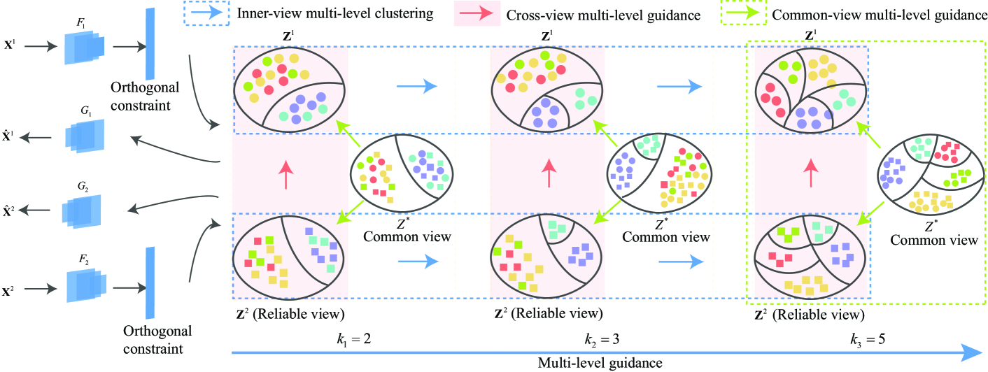
Figure 2: The framework of Multi-level Reliable Guidance for UMC, which is built upon autoencoders with regularization. In the latent space, three stages of training are conducted with $k_{1},k_{2},$ and $k_{3}$, respectively. On each level, three modules are incorporated: the inner-view multi-level clustering module, the cross-view multi-level guidance module, and the common-view multi-level guidance module.

Multi-view autoencoders with regularizer. Autoencoder [41] serves as a prevalent unsupervised model for projecting raw features into a latent feature space, facilitating the learning of view-specific information. Typically, an autoencoder includes an encoder and a decoder. For a given feature representation $\boldsymbol{X}^{v}$ in the v-th view, we utilize an autoencoder to derive the latent representation $\boldsymbol{Z}^{v}$ by minimizing the reconstruction loss. To enhance the discriminative of the latent representation $\boldsymbol{Z}^{v}$, an orthogonal constraint is applied, preventing it from expanding arbitrarily within the integral space [48] and promoting a more discriminative representation [49]. Consequently, for the feature representation $\boldsymbol{X}^{v}$ in the v-th view, we pass it through an autoencoder with a regularizer [7, 8], aiming to learn the latent representation $\boldsymbol{Z}^{v}$ by minimizing the following loss:

$$l_{AE}=\sum_{v=1}^{V}||\boldsymbol{X}^{v}-G^{v}\big{(}F^{v}(\boldsymbol{X}^{v})\big{)}||_{F}^{2}+\lambda_{1}||\boldsymbol{Z}^{v}{\boldsymbol{Z}^{v}}^{T}-\boldsymbol{I}_{d}||_{F}^{2},\\$$ (1)

where $F^{v}$ and $G^{v}$ represent the encoder and decoder of the v-th autoencoder, respectively. $\boldsymbol{Z}^{v}$ is the latent representation of $\boldsymbol{X}^{v}$. $\lambda_{1}$ is a hyperparameter for adjusting the balance between the reconstruction loss and regularizer loss.

III-B Methodology

Multi-level clustering. Due to the absence of supervised information in clustering, cluster assignments can easily change, especially for boundary samples. To mitigate the impact of these boundary samples, various strategies can be employed, such as adaptive weighting [8, 50, 51, 52] and progressive sampling [53, 54]. Sample weights are assigned based on the distance or similarity between samples and cluster centroids. Typically, the weights of boundary samples are set to small values to minimize their influence. However, identifying a sample as a boundary sample using only a single level may be questionable. Additionally, the initial cluster assignment is often unreliable due to insufficient training. Therefore, we consider multi-level clustering with ‘rough classification’ to reduce the negative effect of boundary samples and the error assignment of samples in the beginning.

Specifically, we leverage the concept of super-class [47, 55, 56] to construct the multi-level cluster structure. On each layer, the strategy encourages the samples to stay closer to the distribution of their corresponding super-class than those of others. Compared to direct pseudo-label assignment, the super-class clusters ‘roughly categorize’ samples, providing a softer approach and effectively reducing cluster errors. Therefore, multi-level cluster structure makes boundary samples, which are more prone to being misclassified, more robust in the clustering task of training step by step.

Inner-view multi-level clustering. In each view, samples can be grouped into clusters based on their similarity/distance to different cluster centroids. However, without supervised information, the clustering assignments are inherently uncertain. In multi-view clustering, the more accurately the relationships between samples are captured, the more precisely the clustering distribution can be characterized, thus leading to an effective learning of the clustering structure. To achieve a clear and precise cluster structure, rather than selecting high-confidence samples the same as scl-UMC [8], we utilize high-confidence sample pairs for training in contrastive learning.

Similar to scl-UMC [8], samples within the same cluster are positive pairs, while samples within the different cluster assignments are negative pairs. Furthermore, we define the true pairs and false pairs on these positive pair and negative pair samples via changeless relationships across multiple levels. Specifically, for the positive pairs, those maintaining consistent correlations across different levels are considered true positive pairs, while pairs with varying correlations are labeled as false positive pairs. Similarly, for the negative pairs, those exhibiting constant correlations across multiple levels are identified as true negative pairs, while those with inconsistent correlations are labeled as false negative pairs.

Therefore, to enhance the robustness of the cluster structure, high-confidence sample pairs, consisting of samples in true positive and true negative pairs, participate in the training of contrastive learning. To construct the correlation between samples, we first compute the similarity of samples $\boldsymbol{z}^{v}_{i}$ and $\boldsymbol{z}^{v}_{j}$ by cosine similarity:

$$s^{v}_{ij}=\frac{\boldsymbol{z}^{v}_{i}\boldsymbol{z}^{{v}^{\top}}_{j}}{||\boldsymbol{z}^{v}_{i}||\cdot||\boldsymbol{z}^{v}_{j}||},$$ (2)

where $s^{v}_{ij}$ represents the similarity between sample $\boldsymbol{z}^{v}_{i}$ and $\boldsymbol{z}^{v}_{j}$. Similarly, we set the super-class set as [47], e.g., $k\in\{k_{1},k_{2},k_{3}\}$. Then, the similarities of true positive pairs $tp_{in}(\boldsymbol{z}_{i}^{v})$, and true negative pairs $tn_{in}(\boldsymbol{z}_{i}^{v})$, of $\boldsymbol{z}_{i}^{v}$ in the inner-view with three levels are written as:

$$\begin{split}tp_{in}(\boldsymbol{z}_{i}^{v})=&\{s_{ij}^{v}:j=1,2,\ldots,m_{i}^{v},j\neq i,\\ &c({\boldsymbol{z}^{v,k_{1}}_{i}})\cap c({\boldsymbol{z}^{v,k_{2}}_{i}})\cap c({\boldsymbol{z}^{v,k_{3}}_{i}})\},\\ tn_{in}(\boldsymbol{z}_{i}^{v})=&\{\widetilde{s_{ij}^{v}}:j=1,2,\ldots,n_{i}^{v},j\neq i,\\ &nc({\boldsymbol{z}^{v,k_{1}}_{i}})\cap nc({\boldsymbol{z}^{v,k_{2}}_{i}})\cap nc({\boldsymbol{z}^{v,k_{3}}_{i}})\}.\\ \end{split}$$ (3)

where $c(\boldsymbol{z}^{v,k_{1}}_{i})$ and $nc(\boldsymbol{z}^{v,k_{1}}_{i})$ represent the sets of samples sharing the same and different cluster assignments as $\boldsymbol{z}^{v}_{i}$ with $k_{1}$ clusters, respectively. $m_{i}^{v}$ and $n_{i}^{v}$ denote the number of true positive pairs and true negative pairs, respectively, in the $v$-th view, intersecting across three different cluster numbers.

With the assistance of high-confidence sample pairs (true positive and true negative pairs), there is no need to set a threshold for selecting confident samples. Then, we employ the NT-Xent contrastive loss [57] in all views to learn the reliable cluster structure as follows:

$$l_{in}=\frac{1}{V}\sum_{v=1}^{V}\sum_{i=1}^{n^{v}}\sum_{j=1}^{m_{i}^{v}}\frac{1}{n^{v}m_{i}^{v}}{l}_{ij}^{v},$$ (4)

where

$$l_{ij}^{v}=-\log\frac{\exp{(s_{ij}^{v}/\tau)}}{\sum_{\widetilde{s_{ij}^{v}}\in tn_{in}(\boldsymbol{z}_{i}^{v})}\exp({\widetilde{s_{ij}^{v}}/\tau})}.$$ (5)

$n^{v}$ is the number of samples in the $v$-th view, and $m^{v}_{i}$ is the number of true positive pairs of $\boldsymbol{z}^{v}_{i}$, i.e., $m^{v}_{i}=|tp_{in}(\boldsymbol{z}_{i}^{v})|$. $tn_{in}(\boldsymbol{z}_{i}^{v})$ is the set of true negative sample pairs of $\boldsymbol{z}_{i}^{v}$. $\tau$ is the temperature parameter set to 0.1.

Common-view multi-level guidance. Each view has its specific feature representation and cluster structure, making it challenging to directly align the cluster structures of different views. Therefore, an auxiliary view (common view) is introduced to align different views, thereby reducing the disparities and uncertainty in cluster structures among different views. In our work, the common view $\boldsymbol{Z}^{*}$ is concatenated as $[\boldsymbol{Z}^{1};\ldots;\boldsymbol{Z}^{V}]$. To eliminate variation in cluster structure across views, we align each single view $\{\boldsymbol{Z}^{v}\}_{v=1}^{V}$ with the common view $\boldsymbol{Z}^{*}$ by contrastive learning, thereby helping to merge consistent cluster structures between views.

Specifically, the positive sample pairs are samples with matching cluster centroids between a single view and the common view, while negative sample pairs are samples with non-matching cluster centroids [8]. Therefore, it is crucial to establish the pairing relationships between the cluster centroids of individual views and the common view beforehand. Firstly, we obtain the cluster centroids $\boldsymbol{C}^{v}$ and $\boldsymbol{C}^{*}$ from the single view and the common view using $K$-means. Then, we calculate the weight (cost) matrix $M^{v}$ using $\frac{\boldsymbol{C}^{*}(\boldsymbol{C}^{v})^{\top}}{||\boldsymbol{C}^{*}||\cdot||(\boldsymbol{C}^{v})^{\top}||}$. To acquire the matching relationship, we transform the task of finding pairs of cluster centroids from two views into maximum-weight matchings in a bipartite graph [8, 58, 59]. Naturally, the matching relationship of cluster centroids $\boldsymbol{A}^{v}$ between the common representation $\boldsymbol{Z}^{*}$ and the single view $\{\boldsymbol{Z}^{v}\}_{v=1}^{V}$ is solved by the Hungarian Algorithm [8] as follows:

$$\begin{split}&{\max_{\boldsymbol{A}^{v}}\sum_{i=1}^{K}\sum_{j=1}^{K}{m}^{v}_{ij}{a}^{v}_{ij},}\\ s.t.\boldsymbol{A}^{v}&{\boldsymbol{A}^{v}}^{\top}=\mathbf{I}_{K},\boldsymbol{A}^{v}\in\{0,1\}^{K\times K}\\ \end{split}$$ (6)

where ${m}_{ij}^{v}\in\boldsymbol{M}^{v}$, ${a}^{v}_{ij}\in\boldsymbol{A}^{v}$. Then, the correlation of matched clusters in different views with a common representation is obtained. Finally, we calculate the similarity of $\boldsymbol{z}_{i}^{*}$ and $\boldsymbol{z}_{j}^{v}$ with cosine similarity ${s}^{*v}_{i,j}={\boldsymbol{z}_{i}^{*}\boldsymbol{z}_{j}^{v^{\top}}}/({||\boldsymbol{z}_{i}^{*}||\cdot||\boldsymbol{z}_{j}^{v}||}).$ Then the positive similarity set and negative similarity set of $\boldsymbol{z}_{i}^{*}$ are constructed as follows:

$$\begin{split}&pos_{cro}(\boldsymbol{z}_{i}^{*})=\{s_{ij}^{*v}:v=1,2,\ldots,V,j=1,2,\ldots,n^{v},a^{v}_{ij}=1\},\\ &neg_{cro}(\boldsymbol{z}_{i}^{*})=\{\widetilde{s_{ij}^{*v}}:v=1,2,\ldots,V,j=1,2,\ldots,n^{v},a^{v}_{ij}=0\},\end{split}$$ (7)

where $s_{ij}^{*v}$ and $\widetilde{s_{ij}^{*v}}$ are the similarities of $\boldsymbol{z}_{i}^{*}$ and $\boldsymbol{z}_{j}^{v}$ in positive pairs and negative pairs, respectively. $a^{v}_{i,j}=1$ denotes that the cluster of $\boldsymbol{z}_{i}^{*}$ in the common view matches the cluster of $\boldsymbol{z}_{j}^{v}$ in the $v$-th view, and vice versa for $a^{v}_{i,j}=0$. Therefore, the common-view contrastive learning is formed as follows:

$$l_{co}=\frac{1}{NV}\sum_{i=1}^{N}\sum_{v=1}^{V}\sum_{j=1}^{n^{v}}\frac{1}{n^{v}}{l}^{*v}_{i,j},$$ (8)

where

$${l}^{*v}_{i,j}=-\log\frac{\exp(s_{i,j}^{*v}/\tau)}{\sum_{\widetilde{s_{i,j}^{*v}}\in neg_{cro}}\exp({\widetilde{s_{i,j}^{*v}}/\tau})}.$$ (9)

$n^{v}$ is the number of samples in the $v$-th view. $\tau$ is the temperature parameter, which is set as 0.1.

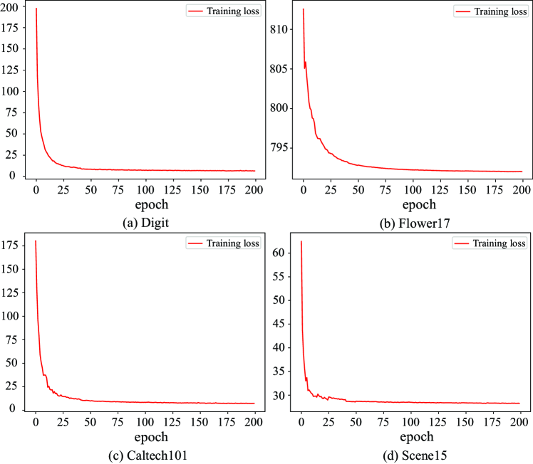
Figure 3: The curve of training loss on MRG-UMC with four datasets.

Cross-view multi-level guidance. Since clustering performance differs among views, the reliability of these views varies. Same as RG-UMC [9] and T-UMC [60], reliable views are those with a silhouette coefficient higher than that of the current view. For the silhouette coefficient of a view, it is defined as:

$$sils^{v}=\frac{1}{n^{v}}\sum_{i=1}^{n^{v}}sil(\boldsymbol{z}_{i}^{v}),$$ (10)

where $sil(\boldsymbol{z}_{i}^{v})$ is the silhouette coefficient of sample $\boldsymbol{z}_{i}^{v}$ [60]. We assume that views with good clustering performance guide the cluster structure formulation of the other views [9].

However, in the early stages of training, due to the lower confidence in the cluster structure and the low silhouette coefficient of all views, only the most reliable views are suitable for training. As training goes on, confidence in multiple views gradually increases, and the silhouette coefficients for each view also rise, allowing more reliable views to participate in training.

Consequently, we leverage a decreasing coefficient $\tau$ to dynamically select reliable views. Specifically, the initial coefficient $\tau$ is set to 1.5 with a decay rate of 0.99 applied at each epoch until the coefficient reaches 1. The reliable views are those whose silhouette coefficient exceeds $\tau$ times that of the current view, and the set of these reliable views is denoted as $\mathcal{C}$. Therefore, the loss of cross-view multi-level guidance is formulated using KL divergence as follows:

$$l_{cr}=\sum_{v=1}^{V}\sum_{r=1}^{|\mathcal{C}|}\frac{1}{V^{2}}P^{v}\text{log}(\frac{P^{v}}{Q^{r}}),$$ (11)

where the indexes of reliable view and current view are $r$ and $v$, respectively. $|\mathcal{C}|$ is the number of reliable views than $v$-th view. $P^{v}$ and $Q^{r}$ are the approximate probability distribution corresponding to the $v$-th view and the $r$-th view.

In sum, to enhance the confidence of clustering structures and matching relationships, the MRG-UMC model is formulated as follows:

$$L=l_{AE}+\lambda_{2}l_{in}+\lambda_{3}l_{co}+\lambda_{4}l_{cr},\\$$ (12)

where $l_{AE}$, $l_{in}$, $l_{co}$ and $l_{cr}$ are the terms of an autoencoder network with orthogonal constraint, inner-view multi-level clustering module, common-view multi-level guidance module, and cross-view multi-level guidance module, respectively. Besides, $\lambda_{2}$, $\lambda_{3}$, and $\lambda_{4}$ are the hyperparameters to balance these modules.

Implementation Details. As shown in Fig.2, the autoecoder structure employed in our work is the same as [61, 8], where each layer includes a batch normalization layer and a Relu layer. For training, we set the maximum number of epochs to 200 and employ mini-batch gradient descent. Specifically, the cluster set $Cs$ is $\{2,\lceil K/2\rceil,K\}$ as in [47] for all datasets, where $K$ is the actual number of clusters. After training is completed, the entire set of unpaired samples is fed into the autoencoder network using the saved parameters to obtain the final feature representation $\{\boldsymbol{Z}^{v}\}_{v=1}^{V}$. Then, we obtain the clustering result by couducting $K$-means on the concatenated representation $\boldsymbol{Z}=[\boldsymbol{Z}^{1};\boldsymbol{Z}^{2};\ldots;\boldsymbol{Z}^{V}]$.

Convergence analysis. The full algorithm for MRG-UMC is provided in Algorithm 1. Additionally, we conduct experiments on four datasets (Digit, Flower17, Caltech101-20 and Scene-15) to demonstrate the convergence of MTG-UM, as depicted in Fig. 3. From Fig. 3, we observed that the loss of MRG-UMC converges rapidly and steadily in fewer than 200 iterations.

Algorithm 1 Proposed MRG-UMC

Input: unpaired multi-view data $\{X^{v}\}_{v=1}^{V}$, the cluster number $K$, $epoch$, $batchsize$, cluster set $Cs$, hyper-parameters $\lambda_{1},\lambda_{2},\lambda_{3},\lambda_{4}$.
Output: clustering assignment.

1:  for $t\leftarrow$ 1 to $epoch$  do

2:     for b $\leftarrow$ 1 to $\lceil N/batchsize\rceil$ do

3:        if $t\leq$ epoch/4 then

4:           $Cs=\{k_{1}\}$

5:        else if $t>$ epoch/4 & $t\leq$ epoch/2 then

6:           $Cs=\{k_{1},k_{2}\}$

7:        else if $t>$ epoch/2 then

8:           $Cs=\{k_{1},k_{2},k_{3}\}$

9:        end if

10:        Update the autoencoder parameter $\{F\}_{v=1}^{s}$ and $\{G\}_{v=1}^{s}$ by minimizing the total loss $L$ in Eq. (12).

11:     end for

12:  end for

13:  Conduct $K$-means on the concatenation $\boldsymbol{Z}=[\boldsymbol{Z}^{1};\boldsymbol{Z}^{2};\ldots;\boldsymbol{Z}^{V}]$ to achieve the final clustering assignment.

IV Experiments

In this section, we compare our model MRG-UMC with 20 comparison methods followed by ablation studies, visualization, and other experiments to validate the effectiveness of multi-level reliable guidance in our work.

Due to space constraints, some information, including experimental settings, network architectures, and 5 benchmark multi-view datasets (Digit, Scene-15, Caltech101-20, Flower17, and Reuters), as well as 20 state-of-the-art compared methods, can be found in [8, 9]. Specifically, these comparison methods include seven complete MC methods (OPMC [62], OP-LFMVC [63], DUA-Nets [64], RMVC[65], DSMVC [66], AWMVC [67] and UOMvSC [68]), eight IMC methods (DAIMC [69], UEAF [70], IMSC-AGL [71], OMVC [72], OPIMC [73], FCMVC [74], T-UMC [60], and GIGA [75]), and five UMC methods (IUMC-CA [7], IUMC-CY [7], scl-UMC [8], RG-UMC [9], and RGs-UMC [9]).

IV-A Performance Comparison and Analysis

TABLE II: Comparison of related multi-view clustering methods for unpaired multi-view clustering. The cells represent the results of NMI, accuracy (ACC) and F1-score (F1) in percentage.

Methods	Digit (6views)			Scene-15 (3views)			Caltech101-20 (6views)			Flower17 (7views)			Reuters (5views)
	NMI	ACC	F1	NMI	ACC	F1	NMI	ACC	F1	NMI	ACC	F1	NMI	ACC	F1
OPMC[62]	12.31	18.33	17.42	17.23	18.94	14.01	12.42	14.30	14.69	13.52	13.38	10.14	11.11	19.48	20.41
OP-LFMVC[63]	22.54	11.57	19.90	9.73	17.02	11.02	13.38	17.34	13.56	9.71	14.88	8.02	-	-	-
DAU-Nets[64]	17.10	19.40	16.82	22.62	21.52	16.30	24.50	15.34	17.90	14.84	13.81	10.77	2.20	25.06	22.98
RMVC[65]	22.31	26.25	17.88	28.84	24.68	18.03	21.72	18.90	17.34	19.08	17.28	11.24	-	-	-
DSMVC[66]	13.95	16.50	7.80	19.86	19.38	10.09	19.44	14.71	2.60	13.55	12.50	4.57	1.53	19.06	15.12
AWMVC [67]	12.72	18.65	14.79	20.95	22.08	15.08	22.32	17.23	18.10	14.17	13.68	9.04	2.57	23.44	24.01
UOMvSC [68]	15.51	18.85	18.17	26.59	24.55	16.75	24.48	16.64	17.50	14.70	13.09	10.99	-	-	-
DAIMC [69]	18.17	25.68	17.96	12.49	19.46	18.68	12.49	19.46	18.68	8.56	12.75	9.83	-	-	-
UEAF[70]	10.32	19.25	16.63	11.59	15.65	12.56	9.28	27.03	24.26	3.91	7.54	10.74	-	-	-
IMSC-AGL[71]	24.01	17.61	17.38	16.45	20.88	12.99	17.30	15.81	12.97	12.66	14.93	8.69	-	-	-
OMVC[72]	12.02	20.03	16.70	11.53	16.09	11.74	18.29	19.26	17.31	12.68	14.68	9.13	-	-	-
OPIMC [73]	20.13	27.74	19.66	15.48	20.33	13.35	17.10	20.18	16.71	11.76	16.39	8.87	10.92	27.46	26.13
FCMVC [74]	12.39	22.55	14.91	9.32	17.15	10.17	9.73	13.29	10.28	8.05	14.59	7.46	5.46	24.93	21.74
T-UMC[60]	9.09	17.70	15.06	26.51	27.65	22.91	11.95	14.08	9.01	11.66	15.74	13.57	-	-	-
GIGA [75]	8.84	17.50	18.95	15.45	16.48	15.67	21.16	16.26	13.03	15.73	15.00	15.40	-	-	-
IUMC-CA[7]	75.16	54.53	60.82	50.25	34.98	34.47	58.31	33.42	33.24	66.13	48.52	44.19	-	-	-
IUMC-CY[7]	74.64	60.72	61.17	56.75	30.58	35.34	61.48	46.63	45.06	63.23	49.21	40.19	10.07	22.99	21.48
scl-UMC[8]	72.75	60.00	50.97	49.62	39.15	33.51	59.63	57.94	60.93	65.65	49.93	47.80	30.73	52.83	31.32
RG-UMC	77.37	84.85	84.65	49.23	53.82	49.82	65.81	67.05	38.92	58.57	50.04	47.81	30.93	59.78	34.54
RGs-UMC	86.19	92.83	92.77	47.40	53.50	48.11	70.88	75.28	41.50	60.64	52.02	51.68	32.26	57.24	33.35
MRG-UMC	88.36	93.99	93.92	49.42	53.88	50.47	72.82	76.48	42.01	61.76	54.85	53.33	40.71	58.29	37.47

The clustering performance of comparison methods. We compare our model with 16 comparison methods on five multi-view datasets and the clustering performance is reported in TABLE II. From TABLE II, we have the following observations:

1) Compared with complete MC and IMC methods, our model, MRG-UMC, outperforms all the comparison methods, demonstrating its effectiveness in UMC. In UMC, the absence of paired samples between views hinders the ability of these comparative methods to explore inter-view relationships, ultimately reducing them to single-view models. This is the reason why these methods perform worse. Fortunately, MRG-UMC constructs relationships between views through multi-level clustering and consistent cluster structures, which help in learning effective representations.

2) Compared with the five UMC methods, our model demonstrates superior performance across most evaluation metrics, indicating a positive effect on performance improvement. Specifically, MRG-UMC achieves an average improvement of 3.42% in NMI, 1.56% in ACC, and 1.86% in F-score compared to the best state-of-the-art method (RGs-UMC), highlighting the effectiveness of our method. For RGs-UMC, although it considers reliable views guidance, it overlooks the confidence of the cluster structures of these views.

IV-B Ablation Study and parameter analysis

Ablation study of MRG-UMC. To further analyze the modules in MRG-UMC, we conducted ablation studies on four datasets (Digit, Scene-15, Caltech101-20 and Flower17). Specifically, we evaluated different combinations of the orthogonal constraint ($Orth$), the inner-view multi-level clustering ($In$), the common-view multi-level guidance module ($Co$), and the cross-view multi-level guidance module ($Cr$). The results of the ablation studies are presented in TABLE III.

As observed from TABLE III, the combination of all modules performs the best (Line 12), which is our method MRG-UMC. In detail, when comparing Lines 2-5 with Line 1, it is evident that the $Cr$ module has the most significant impact on clustering, validating the importance of aligning views through reliable view guidance. Subsequently, the following ablations are based on the $Cr$ module. Taking the Digit dataset as an example, when comparing Lines 6-8 with Line 5, it is evident that the $Orth$ module and $Co$ module are more effective than the $In$ module in learning the cluster structure. The $Orth$ module aids in learning discriminative features, while the $Co$ module facilitates the learning of common feature representations. Both of them help to merge the consistent and discriminative cluster structures between views. Besides, the $In$ module helps to merge trust clustering on each view. Moreover, a comparison between Lines 9-11 and Lines 6-8 reveals that these three modules complement each other, resulting in enhanced performance. The same conclusion can also be drawn from other datasets in TABLE III.

TABLE III: Ablation study of MRG-UMC on four datasets.

Line	Orth	In	Co	Cr	Digit (6views)			Scene-15 (3views)			Caltech101-20 (6views)			Flower17 (7views)
					NMI	ACC	F1	NMI	ACC	F1	NMI	ACC	F1	NMI	ACC	F1
1					15.12	20.86	21.19	20.81	20.28	18.44	19.40	23.69	12.57	15.45	13.98	14.20
2	✓				15.23	21.67	22.36	21.40	21.02	19.27	20.48	27.59	13.33	13.48	13.14	13.47
3		✓			15.07	22.07	23.04	21.01	20.37	18.64	18.10	41.39	12.21	11.75	11.61	11.76
4			✓		14.88	21.52	21.92	21.15	21.00	20.44	23.35	21.81	13.86	14.73	14.06	13.10
5				✓	83.04	90.45	90.35	41.44	47.41	42.87	64.14	64.82	34.27	38.95	36.90	36.00
6	✓			✓	85.27	92.07	91.99	42.06	47.84	44.96	70.02	67.35	36.75	56.04	48.66	45.67
7		✓		✓	85.30	92.22	92.12	42.02	46.97	45.73	67.68	65.21	36.51	43.12	38.81	34.42
8			✓	✓	85.44	92.22	92.14	41.48	46.83	43.03	70.42	74.29	38.64	47.52	43.54	40.45
9	✓	✓		✓	85.57	92.47	92.41	43.01	48.11	44.11	70.74	75.49	38.90	55.94	50.50	48.79
10	✓		✓	✓	85.47	92.22	92.13	42.41	50.93	48.13	69.26	70.69	38.21	54.63	49.81	47.00
11		✓	✓	✓	85.84	92.22	92.10	41.09	49.27	45.70	70.78	73.35	39.98	47.57	45.30	43.72
12	✓	✓	✓	✓	88.36	93.99	93.92	46.09	53.08	50.47	72.82	76.48	42.01	61.76	54.85	53.33

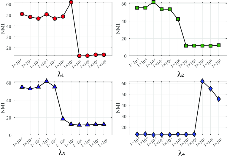
Figure 4: The individual effect of each parameter in MRG-UMC model on clustering performance.

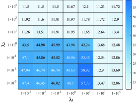
(a) $\lambda_{1}$ and $\lambda_{2}$ in MRG-UMC

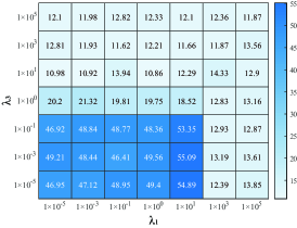
(b) $\lambda_{1}$ and $\lambda_{3}$ in MRG-UMC

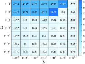
(c) $\lambda_{1}$ and $\lambda_{4}$ in MRG-UMC

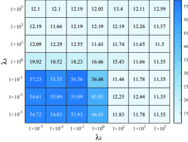
(d) $\lambda_{2}$ and $\lambda_{3}$ in MRG-UMC

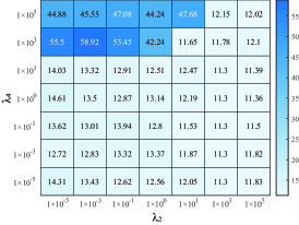
(e) $\lambda_{2}$ and $\lambda_{4}$ in MRG-UMC

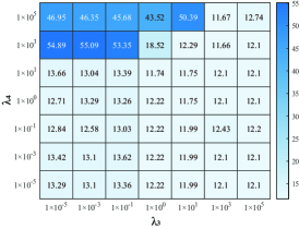
(f) $\lambda_{3}$ and $\lambda_{4}$ in MRG-UMC

Figure 5: Joint effect of the parameters of MRG-UMC model on clustering performance.

Parameter analysis. We analyze the impact of four parameters, $\lambda_{1}$, $\lambda_{2}$, $\lambda_{3}$, and $\lambda_{4}$, in the MRG-UMC model, evaluated on the Flower17 dataset. 1) Individual effects of each parameter. Fig. 4 displays four curves representing NMI values as each parameter varies within the range $\{10^{-5},10^{-4},\ldots,10^{5}\}$ while keeping the remaining parameters fixed at their optimal values. As observed in Fig. 4, $\lambda_{1}$, $\lambda_{2}$, and $\lambda_{3}$ perform well when they are smaller than $10$, $0.1$, and $0.1$, respectively. $\lambda_{4}$ performs well when it is larger than $1000$. Specifically, concerning the orthogonal constraint, higher values of $\lambda_{1}$ significantly degrade performance due to the imposition of hard orthogonality on $\boldsymbol{Z}^{v}$. In the inner-view multi-level clustering, a smaller value of $\lambda_{2}$ facilitates the exploration of relationships between true positive and true negative pairs, while a larger value overly constrains the model, impacting performance. Similarly, in the common-view multi-level guidance module, a small value of $\lambda_{3}$ aids in aligning different views with common views, while a larger value renders the alignment ineffective. In the cross-view multi-level guidance module, a larger value of $\lambda_{4}$ assists in aligning the distribution of different views with reliable views.

2) The joint effect of the parameters. We investigate the joint effect of any two parameters on the Flower17 dataset, as illustrated in Fig. 5 (a)-(f). These parameters vary within the range $\{10^{\text{-5}},10^{\text{-3}},\ldots,10^{3},10^{5}\}$. Regarding the relationship between the orthogonal constraint and the other three modules depicted in Fig. 5 (a)-(c), we observe that the best performance is attained when $\lambda_{1}$ is less than 10. This suggests that imposing a strong orthogonal constraint is not conducive to learning discriminative features. For the relationship between inner-view multi-level clustering and the other three modules in Fig. 5 (a)(d)(e), superior clustering performance is achieved when $\lambda_{2}$ is less than 1. This observation validates the appropriateness of applying a modest constraint on the true positive pairs and true negative pairs in contrastive learning. From Fig. 5 (b)(d)(f), optimal performance is observed when the value of $\lambda_{3}$ is less than $0.1$. When aligning single views to the common view using multi-level methods, a less restrictive constraint proves to be more appropriate. From Fig. 5 (c) and Fig. 5(e)-(f), the best performance is achieved when the $\lambda_{4}$ value is larger than $10$. These observations are consistent with the conclusions from Fig. 4. Furthermore, in all the subfigures in Fig. 5, we observe minor fluctuations in performance within the optimal range for different values. This suggests that these hyperparameters are relatively insensitive to clustering performance.

Single-view performance. MRG-UMC utilizes a consistent cluster structure to connect different views, enabling joint clustering across multiple views. We then evaluated the performance of MRG-UMC on each view across three datasets using $K$-means and compared it with three comparison methods, as shown in TABLE IV. Comparing the $K$-means clustering with the other three methods revealed the effectiveness of cooperative clustering in exploring relationships between views and improving clustering performance. Furthermore, comparing scl-UMC and RGs-UMC with MRG-UMC, we observed significant improvements in clustering performance on each view, which can be attributed to the multi-level reliable guidance strategies.

TABLE IV: The single view cluster performance of MRG-UMC on on four datasets

Dataset	Method	$K$-means			scl-UMC			RGs-UMC			MRG-UMC
	view	NMI	ACC	F1	NMI	ACC	F1	NMI	ACC	F1	NMI	ACC	F1
Digit	v1	44.18	47.27	46.41	47.92	47.27	44.65	53.72	53.94	49.47	88.07	88.79	88.29
	v2	64.49	53.64	51.68	67.92	72.42	73.27	84.04	79.70	77.58	97.63	98.79	98.79
	v3	42.35	48.79	49.19	37.84	49.41	47.78	75.89	84.55	83.99	93.50	96.36	96.23
	v4	61.98	71.21	71.61	57.10	56.36	56.30	85.30	83.33	80.52	97.05	98.48	98.48
	v5	47.87	47.88	46.00	44.17	38.18	35.51	68.00	72.73	71.53	89.84	84.55	82.35
	v6	67.37	65.45	61.75	68.42	64.12	61.65	70.85	71.21	66.24	75.31	76.67	72.03
	all-view	8.57	15.30	15.46	69.73	58.40	52.59	77.37	84.85	84.65	87.18	93.33	93.26
Flower17	v1	50.59	38.50	38.06	53.48	39.57	34.93	59.61	50.80	49.16	73.58	65.24	63.11
	v2	37.73	26.20	25.59	38.81	28.88	26.22	41.34	32.62	30.52	55.91	50.27	48.92
	v3	48.75	37.97	38.36	50.24	39.22	35.92	55.60	43.32	40.71	61.41	49.20	46.52
	v4	44.37	32.09	30.88	42.28	32.09	30.82	50.08	36.90	33.40	63.44	52.94	47.80
	v5	45.63	34.76	34.67	44.78	30.88	30.93	45.19	36.90	37.12	61.43	52.41	51.56
	v6	39.81	33.16	31.34	44.78	30.88	30.93	45.47	35.83	32.54	62.58	50.80	50.76
	v7	45.30	34.76	35.90	40.38	32.35	31.56	47.18	37.43	36.12	67.32	55.61	48.59
	all-view	11.70	12.15	12.51	66.54	50.00	47.06	58.57	50.04	47.81	61.76	54.85	53.33
Caltech101-20	v1	42.81	33.68	27.41	39.61	35.22	26.07	53.86	53.73	31.51	66.95	58.35	39.76
	v2	45.15	33.42	27.46	45.32	37.00	27.98	54.96	44.47	32.31	61.76	46.79	34.33
	v3	45.03	36.76	32.52	43.73	36.09	28.62	54.20	42.67	30.19	65.53	48.59	34.11
	v4	59.86	42.16	31.22	51.98	31.99	25.13	67.99	50.90	36.77	66.18	47.04	32.32
	v5	52.58	38.82	32.52	51.81	40.05	33.49	65.13	47.56	36.71	70.73	64.78	40.58
	v6	59.56	45.50	31.07	54.24	43.28	30.98	62.62	55.78	34.33	70.83	60.93	43.25
	all-view	19.72	15.21	11.08	57.91	38.60	21.95	65.81	67.05	38.92	72.82	76.48	42.01

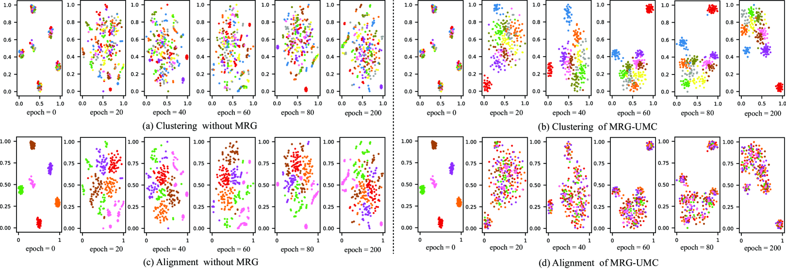
Figure 6: The evolution of the latent representation on Digit dataset, with ten clusters and five views, at intervals of twenty epochs during the training process.

Visualization. To illustrate the efficacy of learning the consistent cluster structure, we employ t-SNE visualization to track the evolution in the latent subspace at intervals of twenty epochs during the training process. Specifically, the experiment is conducted on the Digit dataset with optimal parameters. To show the clustering structure clearly, we randomly sample 500 samples of the latent representation $\boldsymbol{Z}$ and visualize the evolution in Fig. 6 (b) and Fig. 6 (d). Additionally, to clearly demonstrate the effectiveness of MRG-UMC, we conduct visualization experiments without the three modules of MRG-UMC, which are shown in Fig. 6 (a) and Fig. 6 (c). In Fig. 6 (a-b), color represents different cluster assignments predicted by the $K$-means algorithm, while in Fig. 6 (c-d), colors denote different views. Therefore, Fig. 6 (a-b) and (c-d) depict the effectiveness of clustering and alignment, respectively.

From these visualizations, we make the following observations: 1) Comparing Fig. 6 (a) and Fig. 6 (b), we observe that multi-level clustering facilitates the formation of cluster structures, while without these modules, such structures cannot be explored. Similarly, comparing Fig. 6 (c) and Fig. 6 (d), we note that MRG-UMC efficiently and quickly aligns different views. 2) Analyzing Fig. 6 (b), it is apparent that initially, features are mixed, with most samples assigned to a few clusters. However, as training progresses, cluster assignments become more reasonable, and features exhibit clearer gathering and scattering. This observation validates the effectiveness of the MRG-UMC model in learning clear clustering structures. 3) Fig. 6 (d) demonstrates that our methods successfully align samples from different views during training. Initially, samples from different views are separated, but as training goes on, views quickly merge to achieve alignment.

V Conclusion and Future Work

For unpaired multi-view clustering, we propose Multi-level Reliable Guidance for Unpaired Multi-view Clustering (MRG-UMC) to enhance the confidence of cluster structures. MRG-UMC is designed under multi-level clustering and comprises three modules: inner-view multi-level clustering, cross-view multi-level guidance, and common-view multi-level guidance. Our method demonstrates outstanding performance in unpaired multi-view clustering, as supported by comprehensive experiments and analysis.

In our future work, we plan to enhance the robustness of multi-view models. For the ever-changing reality, ensuring the reliability, security, and cleanliness of data becomes increasingly challenging. Furthermore, while many methods aim to enhance overall performance, they often neglect weaker performance on individual views. Consequently, we will further investigate algorithms within stable and secure frameworks. Additionally, we will pay close attention to the application scenarios of unpaired multi-view clustering methods.

References

- [1] C. Xu, D. Tao, and C. Xu, “A survey on multi-view learning,” arXiv preprint arXiv:1304.5634, 2013.
- [2] W. Yang, Y. Gao, Y. Shi, and L. Cao, “Mrm-lasso: A sparse multiview feature selection method via low-rank analysis,” IEEE transactions on neural networks and learning systems, vol. 26, no. 11, pp. 2801–2815, 2015.
- [3] Y. Yang, H. Wei, H. Zhu, D. Yu, H. Xiong, and J. Yang, “Exploiting cross-modal prediction and relation consistency for semisupervised image captioning,” IEEE Transactions on Cybernetics, 2022.
- [4] Y. Yang, J.-Q. Yang, R. Bao, D.-C. Zhan, H. Zhu, X.-R. Gao, H. Xiong, and J. Yang, “Corporate relative valuation using heterogeneous multi-modal graph neural network,” IEEE Transactions on Knowledge and Data Engineering, vol. 35, no. 1, pp. 211–224, 2021.
- [5] C. Xu, D. Tao, and C. Xu, “Multi-view learning with incomplete views,” IEEE Transactions on Image Processing, vol. 24, no. 12, pp. 5812–5825, 2015.
- [6] Y. Yang, D.-C. Zhan, X.-R. Sheng, and Y. Jiang, “Semi-supervised multi-modal learning with incomplete modalities.” in IJCAI, 2018, pp. 2998–3004.
- [7] W. Yang, L. Xin, L. Wang, M. Yang, W. Yan, and Y. Gao, “Iterative multiview subspace learning for unpaired multiview clustering,” IEEE Transactions on Neural Networks and Learning Systems, pp. 1–15, 2023.
- [8] L. Xin, W. Yang, L. Wang, and M. Yang, “Selective contrastive learning for unpaired multi-view clustering,” IEEE Transactions on Neural Networks and Learning Systems, pp. 1–15, 2023.
- [9] L. Xin, W. Yang, L. Wang, and Yang-Ming, “Unpaired multi-view clustering via reliable view guidance,” arXiv preprint arXiv:2404.17894, 2024.
- [10] Y. Wen, S. Wang, Q. Liao, W. Liang, K. Liang, X. Wan, and X. Liu, “Unpaired multi-view graph clustering with cross-view structure matching,” IEEE Transactions on Neural Networks and Learning Systems, 2023.
- [11] Y. Yang and H. Wang, “Multi-view clustering: A survey,” Big Data Mining and Analytics, vol. 1, no. 2, pp. 83–107, 2018.
- [12] N. Sohoni, J. Dunnmon, G. Angus, A. Gu, and C. Ré, “No subclass left behind: Fine-grained robustness in coarse-grained classification problems,” Advances in Neural Information Processing Systems, vol. 33, pp. 19 339–19 352, 2020.
- [13] J. Wen, Z. Zhang, Z. Zhang, L. Zhu, L. Fei, B. Zhang, and Y. Xu, “Unified tensor framework for incomplete multi-view clustering and missing-view inferring,” in Proceedings of the AAAI conference on artificial intelligence, vol. 35, no. 11, 2021, pp. 10 273–10 281.
- [14] G.-Y. Zhang, D. Huang, and C.-D. Wang, “Unified and tensorized incomplete multi-view kernel subspace clustering,” IEEE Transactions on Emerging Topics in Computational Intelligence, pp. 1–17, 2024.
- [15] S. Wang, J. Cao, F. Lei, J. Jiang, Q. Dai, and B. W.-K. Ling, “Multiple kernel-based anchor graph coupled low-rank tensor learning for incomplete multi-view clustering,” Applied Intelligence, vol. 53, no. 4, pp. 3687–3712, 2023.
- [16] C. Zhang, J. Wei, B. Wang, Z. Li, C. Chen, and H. Li, “Robust spectral embedding completion based incomplete multi-view clustering,” in Proceedings of the 31st ACM International Conference on Multimedia, 2023, pp. 300–308.
- [17] L. Li, Z. Wan, and H. He, “Incomplete multi-view clustering with joint partition and graph learning,” IEEE Transactions on Knowledge and Data Engineering, vol. 35, no. 1, pp. 589–602, 2021.
- [18] P. Zhu, X. Yao, Y. Wang, M. Cao, B. Hui, S. Zhao, and Q. Hu, “Latent heterogeneous graph network for incomplete multi-view learning,” IEEE Transactions on Multimedia, 2022.
- [19] W. He, Z. Zhang, Y. Chen, and J. Wen, “Structured anchor-inferred graph learning for universal incomplete multi-view clustering,” World Wide Web, vol. 26, no. 1, pp. 375–399, 2023.
- [20] D. Xia, Y. Yang, S. Yang, and T. Li, “Incomplete multi-view clustering via kernelized graph learning,” Information Sciences, vol. 625, pp. 1–19, 2023.
- [21] Q. Yin, S. Wu, and L. Wang, “Unified subspace learning for incomplete and unlabeled multi-view data,” Pattern Recognition, vol. 67, no. 67, pp. 313–327, 2017.
- [22] W. Yang, Y. Shi, Y. Gao, L. Wang, and M. Yang, “Incomplete-data oriented multiview dimension reduction via sparse low-rank representation,” IEEE Transactions on Neural Networks and Learning Systems, pp. 1–16, 2018.
- [23] J. Liu, X. Liu, Y. Zhang, P. Zhang, W. Tu, S. Wang, S. Zhou, W. Liang, S. Wang, and Y. Yang, “Self-representation subspace clustering for incomplete multi-view data,” in Proceedings of the 29th ACM international conference on multimedia, 2021, pp. 2726–2734.
- [24] Y. Yang, D.-C. Zhan, Y.-F. Wu, Z.-B. Liu, H. Xiong, and Y. Jiang, “Semi-supervised multi-modal clustering and classification with incomplete modalities,” IEEE Transactions on Knowledge and Data Engineering, vol. 33, no. 2, pp. 682–695, 2019.
- [25] A. Li, C. Feng, Z. Wang, Y. Sun, Z. Wang, and L. Sun, “Anchor-based sparse subspace incomplete multi-view clustering,” Wireless Networks, pp. 1–12, 2023.
- [26] Q. Q. A, S. C. A, and X. Z. B, “Multi-view classification with cross-view must-link and cannot-link side information,” Knowledge-Based Systems, vol. 54, no. 4, pp. 137–146, 2013.
- [27] L. Houthuys and J. A. K. Suykens, “Unpaired multi-view kernel spectral clustering,” in 2017 IEEE Symposium Series on Computational Intelligence (SSCI), 2017.
- [28] Z. Huang, P. Hu, J. T. Zhou, J. Lv, and X. Peng, “Partially view-aligned clustering,” Advances in Neural Information Processing Systems, vol. 33, pp. 2892–2902, 2020.
- [29] M. Yang, Y. Li, Z. Huang, Z. Liu, P. Hu, and X. Peng, “Partially view-aligned representation learning with noise-robust contrastive loss,” in Proceedings of the IEEE/CVF conference on computer vision and pattern recognition (CVPR), June 2021, pp. 1134–1143.
- [30] M. Yang, Y. Li, P. Hu, J. Bai, J. C. Lv, and X. Peng, “Robust multi-view clustering with incomplete information,” IEEE Transactions on Pattern Analysis and Machine Intelligence, 2022.
- [31] Y. Wang, D. Chang, Z. Fu, J. Wen, and Y. Zhao, “Partially view-aligned representation learning via cross-view graph contrastive network,” IEEE Transactions on Circuits and Systems for Video Technology, 2024.
- [32] J. Jin, S. Wang, Z. Dong, X. Liu, and E. Zhu, “Deep incomplete multi-view clustering with cross-view partial sample and prototype alignment,” in Proceedings of the IEEE/CVF conference on computer vision and pattern recognition, 2023, pp. 11 600–11 609.
- [33] P. Zeng, M. Yang, Y. Lu, C. Zhang, P. Hu, and X. Peng, “Semantic invariant multi-view clustering with fully incomplete information,” IEEE Transactions on Pattern Analysis and Machine Intelligence, 2023.
- [34] A. P. Dempster, “Upper and lower probabilities induced by a multivalued mapping,” in Classic works of the Dempster-Shafer theory of belief functions. Springer, 2008, pp. 57–72.
- [35] G. Shafer, A mathematical theory of evidence. Princeton university press, 1976, vol. 42.
- [36] A. P. Dempster, “A generalization of bayesian inference,” Journal of the Royal Statistical Society: Series B (Methodological), vol. 30, no. 2, pp. 205–232, 1968.
- [37] Z. Han, F. Yang, J. Huang, C. Zhang, and J. Yao, “Multimodal dynamics: Dynamical fusion for trustworthy multimodal classification,” in Proceedings of the IEEE/CVF conference on computer vision and pattern recognition, 2022, pp. 20 707–20 717.
- [38] Y. Geng, Z. Han, C. Zhang, and Q. Hu, “Uncertainty-aware multi-view representation learning,” in Proceedings of the AAAI Conference on Artificial Intelligence, vol. 35, no. 9, 2021, pp. 7545–7553.
- [39] Z. Han, C. Zhang, H. Fu, and J. T. Zhou, “Trusted multi-view classification with dynamic evidential fusion,” IEEE transactions on pattern analysis and machine intelligence, vol. 45, no. 2, pp. 2551–2566, 2022.
- [40] B. Li, Z. Han, H. Li, H. Fu, and C. Zhang, “Trustworthy long-tailed classification,” in Proceedings of the IEEE/CVF Conference on Computer Vision and Pattern Recognition, 2022, pp. 6970–6979.
- [41] J. Xu, H. Tang, Y. Ren, L. Peng, X. Zhu, and L. He, “Multi-level feature learning for contrastive multi-view clustering,” in Proceedings of the IEEE/CVF Conference on Computer Vision and Pattern Recognition, 2022, pp. 16 051–16 060.
- [42] Y. Yang, Y.-F. Wu, D.-C. Zhan, and Y. Jiang, “Deep multi-modal learning with cascade consensus,” in PRICAI 2018: Trends in Artificial Intelligence: 15th Pacific Rim International Conference on Artificial Intelligence, Nanjing, China, August 28–31, 2018, Proceedings, Part II 15. Springer, 2018, pp. 64–72.
- [43] N. Zhu, J. Cao, Y. Liu, Y. Yang, H. Ying, and H. Xiong, “Sequential modeling of hierarchical user intention and preference for next-item recommendation,” in Proceedings of the 13th international conference on web search and data mining, 2020, pp. 807–815.
- [44] C. Cui, Y. Ren, J. Pu, J. Li, X. Pu, T. Wu, Y. Shi, and L. He, “A novel approach for effective multi-view clustering with information-theoretic perspective,” Advances in Neural Information Processing Systems, vol. 36, 2024.
- [45] Y. Zhou, Q. Zheng, Y. Wang, W. Yan, P. Shi, and J. Zhu, “Mcoco: Multi-level consistency collaborative multi-view clustering,” Expert Systems with Applications, vol. 238, p. 121976, 2024.
- [46] H. Wang, W. Zhang, and X. Ma, “Contrastive and adversarial regularized multi-level representation learning for incomplete multi-view clustering,” Neural Networks, vol. 172, p. 106102, 2024.
- [47] G. Gui, Z. Zhao, L. Qi, L. Zhou, L. Wang, and Y. Shi, “Improving barely supervised learning by discriminating unlabeled samples with super-class,” Advances in Neural Information Processing Systems, vol. 35, pp. 19 849–19 860, 2022.
- [48] M.-S. Chen, T. Liu, C.-D. Wang, D. Huang, and J.-H. Lai, “Adaptively-weighted integral space for fast multiview clustering,” in Proceedings of the 30th ACM International Conference on Multimedia, 2022, pp. 3774–3782.
- [49] M.-S. Chen, C.-D. Wang, D. Huang, J.-H. Lai, and P. S. Yu, “Efficient orthogonal multi-view subspace clustering,” in Proceedings of the 28th ACM SIGKDD Conference on Knowledge Discovery and Data Mining, 2022, pp. 127–135.
- [50] J. Shen, Y. Zhang, H. Liang, Z. Zhao, K. Zhu, K. Qian, Q. Dong, X. Zhang, and B. Hu, “Depression recognition from eeg signals using an adaptive channel fusion method via improved focal loss,” IEEE Journal of Biomedical and Health Informatics, 2023.
- [51] Z. Liu, H. Huang, and S. Letchmunan, “Adaptive weighted multi-view evidential clustering,” in International Conference on Artificial Neural Networks. Springer, 2023, pp. 265–277.
- [52] R. He, Z. Han, Y. Yang, and Y. Yin, “Not all parameters should be treated equally: Deep safe semi-supervised learning under class distribution mismatch,” in Proceedings of the AAAI Conference on Artificial Intelligence, vol. 36, no. 6, 2022, pp. 6874–6883.
- [53] Y. Yang, Y. Zhang, X. Song, and Y. Xu, “Not all out-of-distribution data are harmful to open-set active learning,” Advances in Neural Information Processing Systems, vol. 36, 2024.
- [54] Y. Yang, N. Jiang, Y. Xu, and D.-C. Zhan, “Robust semi-supervised learning by wisely leveraging open-set data,” IEEE Transactions on Pattern Analysis and Machine Intelligence, pp. 1–15, 2024.
- [55] B. Zhang, Y. Wang, W. Hou, H. Wu, J. Wang, M. Okumura, and T. Shinozaki, “Flexmatch: Boosting semi-supervised learning with curriculum pseudo labeling,” Advances in Neural Information Processing Systems, vol. 34, pp. 18 408–18 419, 2021.
- [56] K. Sohn, D. Berthelot, N. Carlini, Z. Zhang, H. Zhang, C. A. Raffel, E. D. Cubuk, A. Kurakin, and C.-L. Li, “Fixmatch: Simplifying semi-supervised learning with consistency and confidence,” Advances in neural information processing systems, vol. 33, pp. 596–608, 2020.
- [57] T. Chen, S. Kornblith, M. Norouzi, and G. Hinton, “A simple framework for contrastive learning of visual representations,” in International conference on machine learning. PMLR, 2020, pp. 1597–1607.
- [58] A. Grinman, “The hungarian algorithm for weighted bipartite graphs,” Massachusetts Institute of Technology, 2015.
- [59] D. Bruff, “The assignment problem and the hungarian method,” Notes for Math, vol. 20, no. 29-47, p. 5, 2005.
- [60] J.-Q. Lin, M.-S. Chen, C.-D. Wang, and H. Zhang, “A tensor approach for uncoupled multiview clustering,” IEEE Transactions on Cybernetics, 2022.
- [61] Y. Lin, Y. Gou, Z. Liu, B. Li, J. Lv, and X. Peng, “Completer: Incomplete multi-view clustering via contrastive prediction,” in Proceedings of the IEEE/CVF Conference on Computer Vision and Pattern Recognition (CVPR), June 2021.
- [62] J. Liu, X. Liu, Y. Yang, L. Liu, S. Wang, W. Liang, and J. Shi, “One-pass multi-view clustering for large-scale data,” in Proceedings of the IEEE/CVF International Conference on Computer Vision, 2021, pp. 12 344–12 353.
- [63] X. Liu, L. Liu, Q. Liao, S. Wang, Y. Zhang, W. Tu, C. Tang, J. Liu, and E. Zhu, “One pass late fusion multi-view clustering,” in International Conference on Machine Learning. PMLR, 2021, pp. 6850–6859.
- [64] Y. Geng, Z. Han, C. Zhang, and Q. Hu, “Uncertainty-aware multi-view representation learning,” in Proceedings of the AAAI Conference on Artificial Intelligence, vol. 35, no. 9, 2021, pp. 7545–7553.
- [65] H. Tao, C. Hou, X. Liu, T. Liu, D. Yi, and J. Zhu, “Reliable multi-view clustering,” in Proceedings of the AAAI conference on artificial intelligence, vol. 32, no. 1, 2018.
- [66] H. Tang and Y. Liu, “Deep safe multi-view clustering: Reducing the risk of clustering performance degradation caused by view increase,” in Proceedings of the IEEE/CVF Conference on Computer Vision and Pattern Recognition, 2022, pp. 202–211.
- [67] X. Wan, X. Liu, J. Liu, S. Wang, Y. Wen, W. Liang, E. Zhu, Z. Liu, and L. Zhou, “Auto-weighted multi-view clustering for large-scale data,” in Proceedings of the AAAI Conference on Artificial Intelligence, vol. 37, no. 8, 2023, pp. 10 078–10 086.
- [68] C. Tang, Z. Li, J. Wang, X. Liu, W. Zhang, and E. Zhu, “Unified one-step multi-view spectral clustering,” IEEE Transactions on Knowledge and Data Engineering, vol. 35, no. 6, pp. 6449–6460, 2023.
- [69] M. Hu and S. Chen, “Doubly aligned incomplete multi-view clustering,” in Twenty-Seventh International Joint Conference on Artificial Intelligence IJCAI-18, 2018.
- [70] J. Wen, Z. Zhang, Y. Xu, B. Zhang, L. Fei, and H. Liu, “Unified embedding alignment with missing views inferring for incomplete multi-view clustering,” in Proceedings of the AAAI conference on artificial intelligence, vol. 33, no. 01, 2019, pp. 5393–5400.
- [71] J. Wen, Y. Xu, and H. Liu, “Incomplete multiview spectral clustering with adaptive graph learning,” IEEE Transactions on Cybernetics, vol. 50, no. 4, pp. 1418–1429, 2020.
- [72] W. Shao, L. He, C. T. Lu, and P. S. Yu, “Online multi-view clustering with incomplete views,” in 2016 IEEE International Conference on Big Data, 2016.
- [73] M. Hu and S. Chen, “One-pass incomplete multi-view clustering,” Proceedings of the AAAI Conference on Artificial Intelligence, vol. 33, pp. 3838–3845, 2019.
- [74] X. Wan, B. Xiao, X. Liu, J. Liu, W. Liang, and E. Zhu, “Fast continual multi-view clustering with incomplete views,” IEEE Transactions on Image Processing, vol. 33, pp. 2995–3008, 2024.
- [75] Z. Yang, H. Zhang, Y. Wei, Z. Wang, F. Nie, and D. Hu, “Geometric-inspired graph-based incomplete multi-view clustering,” Pattern Recognition, vol. 147, p. 110082, 2024.