Improving the performance of Stein variational inference through extreme sparsification of physically-constrained neural network models

Abstract

Most scientific machine learning (SciML) applications of neural networks involve hundreds to thousands of parameters, and hence, uncertainty quantification for such models is plagued by the curse of dimensionality. Using physical applications, we show that $L_{0}$ sparsification prior to Stein variational gradient descent ($L_{0}$+SVGD) is a more robust and efficient means of uncertainty quantification, in terms of computational cost and performance than the direct application of SGVD or projected SGVD methods. Specifically, $L_{0}$+SVGD demonstrates superior resilience to noise, the ability to perform well in extrapolated regions, and a faster convergence rate to an optimal solution.

1 Introduction

Quantifying the uncertainty in the parameters of a model and thereby its predictions has become a central thrust in creating models for trustworthy simulation across engineering and science. However, the well-established methods for obtaining posterior distributions of likely parameters such as Markov chain Monte Carlo (MCMC) sampling [1] become infeasible with highly parameterized machine learning function representations, such as neural networks (NNs). The curse of dimensionality in this uncertainty quantification (UQ) setting is tied to the cost of sampling the posterior sufficiently to determine its covariance structure and generate representative push-forward realizations.

In this work, our goal is to obtain a high-dimensional posterior distribution over a large number of random variables representing model parameters, which is particularly useful when limited amount of training data is available. One of the simplest ways to obtain the approximate posterior is to implement MCMC methods. However, this approach is challenged by the number of parameters typically present in NNs and it is difficult to converge samples to those representative of the posterior, even for models with moderate dimensionality. There has been enormous progress made to approximate high-dimensional posterior distributions using variational inference methods [2]. However, these methods restrict the approximate posterior to a certain parametric family and find the best approximate posterior through optimization. To surmount these issues, Liu and Wang [3] recently proposed a non-parametric variational inference method called Stein variational gradient descent (SVGD). Stein variational inference methods [3, 4] and their projected variants [5, 6] address shortcomings in both the reference standard MCMC methods, such as Hamiltonian Monte Carlo (HMC) [7], and the ubiquitous mean field variational inference technique [8, 9] by using an ensemble of particles that represent likely model realizations. In SVGD, these particles simultaneously follow a gradient flow toward the true posterior which is augmented with repulsive forces that keep the realizations distinct. Projected SVGD (pSVGD) starts with a model reduction step based on the Hessian at the maximum a posteriori (MAP) estimate of the posterior distribution to divide the parameter space into an active component and an inactive complement.

Unlike pSVGD which relies on a subspace around the MAP, we propose that model parameter sparsification prior to uncertainty quantification can embed non-linear aspects of the reduction of a fully parameterized NN not captured in a linearization (Laplace-like approximation). After regularization-based sparsification to obtain a reduced dimensionality parameter manifold, the proposed method proceeds with SVGD on the sparsified NN model. We explore the $L_{p}$ family of regularizations including the recently introduced smoothed $L_{0}$ technique [10]. We focus this work on the uncertainty quantification of physical response models, specifically those that admit a potential and other structure, which additionally can be subject to a variety of constraints that we aim to strongly enforce. To this end, we use combinations of sparsification and UQ methods, including pSVGD, full SVGD, $L_{0}$+HMC, and the proposed method ($L_{0}$+SVGD), to demonstrate their relative efficacy in this task.

In the next section, Sec.​ 2, we give the background for the proposed methodology, followed by a description of the algorithms in Sec.​ 3. In Sec.​ 4 we demonstrate these methods on two physical representation problems and compare results obtained via the competing algorithms. Lastly, in Sec.​ 5, we conclude with a summary and directions for future work.

2 Related work

Our work draws on and we compare it to a number of uncertainty quantification, sparsification and machine learning techniques.

Variational inference (VI) is a UQ technique that recasts the UQ problem of constructing a posterior distribution of model parameters as an optimization problem. VI fits a surrogate distribution, typically from a pre-selected family of distributions, to the available data through a Kullback-Liebler divergence measuring the similarity of the surrogate to the true posterior. So-called mean field VI limits the covariance of the surrogate to a diagonal matrix for computational efficiency and hence ignores parameter correlations. Although widely used, this technique is known to generally underestimate uncertainty by construction due to the restricted covariance and the evidence lower bound objective [11]. More recently, Liu and Wang [12] introduced Stein variational gradient descent which employs a coordinated ensemble of model realizations (particles) to sample the covariance structure of the posterior. Due to the limitations of applying this technique to models with a large number of parameters, subsequently Chen et al. [6] developed projected SVGD to handle parameter spaces that have an active subspace of influential parameters.

Sparsification of model parameterizations has had a long history of development [13, 14]. A primary method of sparsification is through regularization of the fitting objective by adding a secondary objective, which allows the model fit to compete with model complexity. Willams [15] introduced the $L_{1}$ regularization prior in the Bayesian setting that promotes sparsity due to the shape of the $L_{1}$ level sets. Later, Louizos et al. [10, 16] introduced a practical $L_{0}$ regularization based on smoothing the counting norm. $L_{0}$ regularization was employed in Fuhg et al. [17] to great effect on physics-augmented models, which are the topic of this work. In addition, Van Baalen et al. [18] applied $L_{0}$ pruning in a Bayesian and precision quantization context for image classification.

Constraints on model structure, such as convexity, remove (parametric) model complexity that violates physical principles. Amos et al. [19] proposed the notion of a input convex neural network (ICNN), which embeds strict convexity in the model formulation. This representation has been widely employed in the computational mechanics community in constructing well-behaved potentials [20, 21, 22, 23, 24, 25, 26, 27, 28] and other constructs such as yield functions [28]. Other properties such as positivity [23, 29] and equivariance [30, 31] can also be embedded in NN formulations.

3 Methods

When given data, it is standard practice in a Bayesian framework to assess the epistemic/reducible parametric uncertainty of a model by first finding a MAP estimate of the parameters and then using this estimate as the starting point for an MCMC sampling procedure [32] of the posterior distribution. Unfortunately, for models with many parameters, such as NNs, the curse of dimensionality prevents simple sampling methods from efficiently characterizing the distribution of likely parameters. More efficient methods, such as those based on VI, have been developed to address this shortcoming. In particular, Stein variational inference attains a degree of parallel efficiency by using a coordinated ensemble of model realizations (particles) to explore the posterior distribution; however, the number of particles to fully characterize the posterior covariance still grows exponentially with the number of parameters. As mentioned, pSVGD interleaves a model reduction step using a linear subspace arrived at through a proper orthogonal-like decomposition. We propose to follow this notion by considering the MAP model structure and then applying Stein variational inference to this reduced dimensionality parameter manifold. We believe this approach will be more effective in accommodating the complex nonlinear dependencies found in many NN models. Of course, this depends on the effectiveness of the regularization scheme, as the premise is that a low-dimensional representation is sufficiently accurate for the physical problem.

3.1 Bayesian calibration

Given a dataset of input-output pairs $\mathcal{D}=\{\mathsf{x}^{i},\mathsf{y}^{i}\}_{i=1}^{N}$, where $N$ is the total number of training data and a model

$$\hat{\mathsf{y}}=\mathsf{N}\!\mathsf{N}(\mathsf{x};{\bm{\theta}})\ ,$$ (1)

Bayes rule provides a foundation for quantifying the uncertainty in the model parameters ${\bm{\theta}}$:

$$\pi({\bm{\theta}}\,|\,\mathcal{D})=\frac{\pi(\mathcal{D}\,|\,{\bm{\theta}})\,\pi({\bm{\theta}})}{\pi(\mathcal{D})}$$ (2)

Here, the posterior $\pi({\bm{\theta}}\,|\,\mathcal{D})$ is proportional to the likelihood $L({\bm{\theta}})=\pi(\mathcal{D}|{\bm{\theta}})$ multiplied by prior $\pi({\bm{\theta}})$, where the evidence $\pi(\mathcal{D})$ is a constant, normalizing factor. The MAP estimate ${\bm{\theta}}^{*}$ is a point estimate given by optimizing the log posterior

$${\bm{\theta}}^{*}=\operatorname{argmax}_{\bm{\theta}}\left[\log\pi({\bm{\theta}}\,|\,\mathcal{D})\right]=\operatorname{argmax}_{\bm{\theta}}\left[\log\pi(\mathcal{D}\,|\,{\bm{\theta}})+\log\pi({\bm{\theta}})\right]$$ (3)

In the absence of specific distributions for the discrepancy between the model and the data, we assume a multivariate normal distribution for the likelihood $L({\bm{\theta}})$, leading to

$$-\log\pi({\bm{\theta}}\,|\,\mathcal{D})=\|\mathsf{y}-\mathsf{N}\!\mathsf{N}(\mathsf{x};{\bm{\theta}})\|_{\bm{\Sigma}}^{2}+\lambda\|{\bm{\theta}}\|_{p}+\text{constant}\ ,$$ (4)

where $\bm{\Sigma}$ is the likelihood covariance that characterizes data noise and is usually taken to be diagonal. In Eq.  (4), we also assumed specific forms for the prior distribution $\log\pi({\bm{\theta}})$ based on regularizing priors. Hence the MAP can be obtained by the optimization of the loss $\mathcal{L}$

$${\bm{\theta}}^{*}=\operatorname{argmin}_{{\bm{\theta}}}\underbrace{\left[\|\mathsf{y}-\mathsf{N}\!\mathsf{N}(\mathsf{x};{\bm{\theta}})\|_{\bm{\Sigma}}^{2}+\lambda\|{\bm{\theta}}\|_{p}\right]}_{\mathcal{L}({\bm{\theta}};\mathcal{D})}$$ (5)

composed of the $\bm{\Sigma}$ weighted mean squared error with a secondary, complexity-reducing regularization objective associated with the prior [15, 33, 34].

The connection between the MAP optimization loss and the log posterior shows how the prior can be identified with a penalization of non-zero parameters. For instance, $L_{2}$ regularization is associated with a Gaussian prior

$$\pi({\bm{\theta}})=\mathcal{N}(\mathbf{0},\sigma^{2}\mathbf{I};{\bm{\theta}})\propto\exp\left(-\frac{\|{\bm{\theta}}\|^{2}_{2}}{2\sigma^{2}}\right)$$ (6)

where $\lambda=\sigma^{-2}$ acts as a penalty parameter in this context; likewise $L_{1}$ penalization corresponds to a Laplace prior

$$\pi({\bm{\theta}})\propto\exp\left(-\lambda\|{\bm{\theta}}\|_{1}\right)$$ (7)

The regularization norm in Eq.  (4), together with the likelihood, determines the sparsification pattern of the parameters in the NN model, i.e. the active and inactive parameters. The goal of sparsification is to reduce the number of parameters while maintaining accuracy. This elimination of redundant parameters can promote generalization and will aid our goal of efficient and accurate uncertainty quantification.

A representation of the posterior itself can be obtained through sampling with MCMC methods like HMC [1] or with Stein variational inference methods like SVGD, which will be discussed in Sec.​ 3.3. With a posterior on the parameters $\pi({\bm{\theta}}\,|\,\mathcal{D})$, we can then evaluate the pushforward distribution of the outputs by sampling the posterior and evaluating the model:

$$\hat{\mathsf{y}}=\mathsf{N}\!\mathsf{N}(\mathsf{x};{\bm{\theta}})\ \text{with}\ {\bm{\theta}}\sim\pi({\bm{\theta}}\,|\,\mathcal{D})\ .$$ (8)

3.2 Smoothed $L_{0}$ sparsification

Sparsification by $L_{0}$ regularization employs the $L_{0}$ norm, also known as the counting norm since it gives the cardinality of a set or vector, which is not differentiable. The smoothed $L_{0}$ approach [10] follows the general idea of a gating system where each trainable parameter is multiplied by a gate value $z\in[0,1]$, which makes the parameter inactive ($z=0$) or active ($z=1$). The number of active gates, and therefore the model complexity, can then be penalized in the loss function. However, due to the binary nature of the gates, this loss function is not differentiable. Hence, following Ref.  [10], we consider a reparametrization of the trainable parameters using a smoothed gating system, i.e. let

$${\bm{\theta}}=\overline{{\bm{\theta}}}\odot\mathsf{z},\quad\text{with}\quad\mathsf{z}=\min(\bm{1},\max(\bm{0},\overline{\bm{s}}))$$ (9)

where $\odot$ denotes the Hadamard product and

$$\overline{\bm{s}} = \bm{s}(\zeta-\gamma)+\gamma\bm{1},$$ (10)

$$\bm{s} = \operatorname{sig}((\log\bm{u}-\log(1-\bm{u})+\log\bm{\alpha})/\beta),$$

Here, $\gamma$, $\beta$, $\zeta$ and $\log\alpha$ are user-chosen hyperparameters that define the smoothing of the vector of gate values $\mathsf{z}$ and $\bm{u}\sim\mathcal{U}(\bm{0},\bm{1})$ is a uniform random vector which is the same dimension as $\mathsf{z}$. Following the suggestions of Ref.  [10], we set $\gamma=-0.1$, $\zeta=1.1$, $\beta=2/3$, and obtain $\log\bm{\alpha}\sim\mathcal{N}(0,\sigma)$ by sampling from a normal distribution with zero mean and $\sigma=0.01$ standard deviation. Since the gate vector is a random vector, we can define a Monte Carlo approximated loss function as

$$\mathcal{R}(\overline{{\bm{\theta}}}) =\frac{1}{M}\sum_{j=1}^{M}\left(\frac{1}{N}\left(\sum_{i=1}^{N}\mathcal{L}\left(\mathsf{N}\!\mathsf{N}\left(\mathsf{x}_{i},\overline{{\bm{\theta}}}\odot\mathsf{z}^{m}\right),\mathsf{y}_{i}\right)\right)\right]$$ (11)

$$+\lambda\sum_{j=1}^{\bm{\theta}}\operatorname{sig}\left(\log\alpha_{j}-\beta\log\frac{-\gamma}{\zeta}\right)\ ,$$

with $M$ being the number of samples of the Monte Carlo approximation and where $\lambda$ is the penalty weighting factor for the regularization analogous to that in Eq.  (4). To make predictions at test time we can then set the values of the trainable parameters ${\bm{\theta}}^{*}=\overline{{\bm{\theta}}}^{*}\odot\hat{\mathsf{z}}$ where the gate values are obtained from

$$\hat{\mathsf{z}}=\min(\bm{1},\max(\bm{0},\operatorname{sig}(\log\bm{\alpha})(\zeta-\gamma)+\gamma\bm{1})).$$ (12)

i.e.negative gate values correspond to inactive parameters.

3.3 Stein variational inference

As mentioned in Sec.​ 3.1, the posterior $\pi({\bm{\theta}}|\mathcal{D})$ given in Eq.  (2) can be sampled using MCMC methods like HMC. However, with a large number of uncertain parameters ${\bm{\theta}}$, using traditional sampling methods can be a formidable challenge to obtain converged statistics due to sampling inefficiency, hyperparameter tuning, and the sequential nature of MCMC sampling. On the other hand, most variational inference methods [11] solve the Bayesian inference problem by minimizing the Kullback-Liebler (KL) divergence between the surrogate distribution $q({\bm{\theta}})$ and the posterior distribution $\pi({\bm{\theta}}\,|\,\mathcal{D})$. The optimization problem is formulated in terms of the KL divergence as follows:

$$q^{*}({\bm{\theta}})=\underset{q\in\mathcal{Q}}{\arg\min}\,{\operatorname{KL}}(q({\bm{\theta}})\|\pi({\bm{\theta}}|\mathcal{D}))=\underset{q\in\mathcal{Q}}{\arg\min}\,\mathbb{E}_{q}[\log q({\bm{\theta}})-\log\tilde{p}({\bm{\theta}}|\mathcal{D})]\ ,$$ (13)

where $\tilde{p}({\bm{\theta}}|\mathcal{D})=\pi(\mathcal{D}|{\bm{\theta}})\pi({\bm{\theta}})=\prod_{i=1}^{N}\pi\left(\mathbf{y}^{i}|{\bm{\theta}},\mathbf{x}^{i}\right)\pi({\bm{\theta}})$ is the unnormalized posterior. The major drawback of this method is that it confines the approximate posterior to specific parametric variational families.

Therefore, we consider a non-parametric variational inference method called Stein variational gradient descent (SVGD) [35]. This method initializes a set of $S$ particles $\{\bm{{\bm{\theta}}}_{0}^{i}\}_{i=1}^{S}$ that represent likely model parameterizations, and then iteratively moves them to the high posterior probability region using gradient information. This update is guided by a step size and a perturbation direction given by the Stein discrepancy, ensuring the transformed particles align more closely with the target posterior, and can be interpreted [35] as a gradient descent algorithm, like Adam [36]. As in Ref.  [3], we employ the closed-form Stein discrepancy:

$$\bm{\phi}^{*}({\bm{\theta}})\propto\mathbb{E}_{{\bm{\theta}}^{{}^{\prime}}\sim\mu}[\mathcal{T}^{{\bm{\theta}}^{{}^{\prime}}}_{\pi}\kappa({\bm{\theta}},{\bm{\theta}}^{{}^{\prime}})]=\mathbb{E}_{{\bm{\theta}}^{{}^{\prime}}\sim\mu}[\nabla_{{\bm{\theta}}^{{}^{\prime}}}\log\pi({\bm{\theta}}^{{}^{\prime}}\,|\,\mathcal{D})\kappa({\bm{\theta}},{\bm{\theta}}^{{}^{\prime}})+\nabla_{{\bm{\theta}}^{{}^{\prime}}}\kappa({\bm{\theta}},{\bm{\theta}}^{{}^{\prime}})],$$ (14)

where $\mathcal{T}_{\pi}$ is the Stein operator, $\kappa(\bm{{\bm{\theta}}},\bm{{\bm{\theta}}^{\prime}})$ is a positive kernel, $\nabla_{{\bm{\theta}}^{\prime}}\log\pi\left({\bm{\theta}}^{\prime}\,|\,\mathcal{D}\right)\kappa\left({\bm{\theta}},{\bm{\theta}}^{\prime}\right)$ is a kernel smoothed gradient, $\nabla_{{\bm{\theta}}}\kappa\left({\bm{\theta}},{\bm{\theta}}^{\prime}\right)$ is a repulsive force, and $\mu$ is the measure associated with the surrogate posterior distribution. In this work, we choose a standard radial basis function kernel in the update procedure summarized in Alg.  1. For more details on SVGD, see A.

Input: A set of initial particles $\{{\bm{\theta}}_{0}^{i}\}_{i=1}^{S}$, score function $\nabla\log\pi({\bm{\theta}}\mid\mathcal{D})$, kernel $\kappa({\bm{\theta}},{\bm{\theta}}^{{}^{\prime}})$, step-size $\{\epsilon_{t}\}$

for iteration t do

       $\bm{\phi}({\bm{\theta}}_{t}^{i})=\frac{1}{S}\sum_{j=1}^{S}\Big{[}\kappa({\bm{\theta}}_{t}^{j},{\bm{\theta}}_{t}^{i})\nabla_{{\bm{\theta}}_{t}^{j}}\log\pi({\bm{\theta}}_{t}^{j},\mathcal{D})+\nabla_{{\bm{\theta}}_{t}^{j}}\kappa({\bm{\theta}}_{t}^{j},{\bm{\theta}}_{t}^{i})\Big{]}$

       ${\bm{\theta}}^{i}_{t+1}$ $\leftarrow$ ${\bm{\theta}}^{i}_{t}+\epsilon_{t}\bm{\phi}({\bm{\theta}}^{i}_{t})$

end for

Result: A set of particles ${\bm{\theta}}^{i}$ that approximates the target posterior

Algorithm 1 Stein variational gradient descent (SVGD) [3].

The projected Stein algorithm [6] propagates gradient descent on a subspace constructed from the likelihood Hessian at the MAP. The subspace is constructed from the most significant generalized eigenvectors of the particle averaged Hessian. The column matrix of the leading eigenvectors allows the projection of parameters into the active low-dimensional subspace where the likelihood informs the posterior more than the prior does. The full-dimensional posterior is then reconstructed by lifting the low-dimensional samples at a given gradient descent step and recombining them with the inactive part of the prior. Alg.  2 summarizes the additional steps of pSVGD.

Input: A set of initial particles $\{{\bm{\theta}}_{0}^{i}\}_{i=1}^{S}$, score function $\nabla\log\pi({\bm{\theta}}\mid\mathcal{D})$, kernel $\kappa({\bm{\theta}},{\bm{\theta}}^{{}^{\prime}})$, step-size $\{\epsilon_{t}\}$

Form Hessian $\mathsf{H}={\bm{\nabla}}_{\bm{\theta}}\left[{\bm{\nabla}}_{\bm{\theta}}L_{\mathsf{y}}({\bm{\theta}})\right]$ at the MAP ${\bm{\theta}}^{*}$.

Solve the eigenvalue problem $\mathsf{H}{\bm{\psi}}_{i}=\lambda_{i}\bm{\Sigma}_{0}^{-1}{\bm{\psi}}_{i}$ where $\bm{\Sigma}_{0}$ is the prior covariance.

Determine the active subspace of the $r$ eigenvectors $\bm{\Psi}=[{\bm{\psi}}_{0},{\bm{\psi}}_{1},\ldots,{\bm{\psi}}_{r}]$ with spectral content 0.99 of the total

Construct the projector $\mathsf{P}=\bm{\Psi}\bm{\Psi}^{T}$

for iteration t do

       $\bm{\phi}({\bm{\theta}}_{t}^{i})=\frac{1}{S}\sum_{j=1}^{S}\Big{[}\kappa({\bm{\theta}}_{t}^{j},{\bm{\theta}}_{t}^{i})\nabla_{{\bm{\theta}}_{t}^{j}}\log\pi({\bm{\theta}}_{t}^{j},\mathcal{D})+\nabla_{{\bm{\theta}}_{t}^{j}}\kappa({\bm{\theta}}_{t}^{j},{\bm{\theta}}_{t}^{i})\Big{]}$

       ${\bm{\nabla}}_{{\bm{\theta}}^{r}_{j}}\log\pi({\bm{\theta}}^{r}_{j}\,|\,\mathcal{D})=\mathsf{P}^{T}{\bm{\nabla}}_{{\bm{\theta}}_{j}}\log\pi({\bm{\theta}}_{j}\,|\,\mathcal{D})$

       ${\bm{\theta}}^{i}_{t+1}$ $\leftarrow$ ${\bm{\theta}}^{i}_{t}+\epsilon_{t}\bm{\phi}({\bm{\theta}}^{i}_{t})$

end for

Reconstruct ${\bm{\theta}}^{i}=\bm{\Psi}{\bm{\theta}}^{i}+{\bm{\theta}}^{*}+{\bm{\theta}}^{i}_{\perp}$ where ${\bm{\theta}}^{i}_{\perp}$ are sampled from the prior and projected by the complement of $\mathsf{P}$

Result: A set of particles ${\bm{\theta}}^{i}$ that approximates the target posterior

Algorithm 2 Projected Stein variational gradient descent (pSVGD) [6].

4 Results

To ameliorate the curse of dimensionality and obtain the posterior distribution of model parameters, we propose first using $L_{0}$ sparsification to find a sparse model structure that approximates the MAP and then using SVGD on this compact parameterization ($L_{0}$+Stein). We compare this methodology to SVGD alone (Alg. 1) and pSVGD (Alg. 2) for UQ of physical NN models using examples from hyperelasticity and mechanochemistry. For the SVGD methods, we explored $L_{0}$, $L_{1}$, and $L_{2}$ regularizations. For these demonstrations, only $L_{0}$ regularization leads to parametrically compact models. The other regularizations can reduce the total number of parameters, especially when combined with constraints on the weights as in ICNNs, but not as effectively as $L_{0}$. For the compact $L_{0}$ hyperelastic model, which had less than 10 parameters, we were able to compare $L_{0}$+Stein to $L_{0}$+HMC results.

To each of the datasets we added multiplicative (heteroskedastic) noise

$$\mathsf{y}={\bm{\eta}}*\hat{\mathsf{y}}(\mathsf{x})$$ (15)

where $\hat{\mathsf{y}}$ is the output of the data generating model and ${\bm{\eta}}\sim\mathcal{N}(\mathbf{0},\sigma^{2}\mathbf{I})$ is independent, identically distributed Gaussian noise mimicking measurement noise. We employed this noise to test the proposed method’s prediction for out-of-training range where the noise level is different than in the training range. Our comparison with HMC is the one exception where we added additive (homoskedastic) noise

$$\mathsf{y}=\hat{\mathsf{y}}(\mathsf{x})+{\bm{\eta}}$$ (16)

to connect to the classical UQ case [37].

For all cases, we compare the push-forward posterior of the output $\mathsf{y}$, as in Eq.  (8). We use the Wasserstein-1 ($W_{1}$) distance to compare these push-forward posteriors estimated by the competing methods to data and to each other

$$\text{W}_{1}(\pi_{a}(X),\pi_{b}(X))=\int|\operatorname{CDF}_{a}-\operatorname{CDF}_{b}|\,\mathrm{d}X$$ (17)

where the cumulative distribution functions (CDFs), associated with the probability density functions $\pi_{a}$, are defined empirically from the samples. As a distance, a smaller $W_{1}$ implies that the two distributions are more similar.

4.1 Hyperelasticity

Hyperelasticity [17] assumes the existence of a potential $\Psi$ such that the stress $\mathbf{S}$ can be derived as

$$\mathbf{S}=2{\bm{\partial}}_{\mathbf{C}}\Psi,$$ (18)

where $\mathbf{C}=\mathbf{F}^{T}\mathbf{F}$ is the left Cauchy-Green deformation tensor and $\mathbf{F}$ is the deformation gradient. Assuming material isotropy implies that the invariants

$$I_{1}=\operatorname{tr}\mathbf{C},\quad I_{2}=\operatorname{tr}\mathbf{C}^{*},\quad J=\sqrt{\det\mathbf{C}}$$ (19)

fully determine $\Psi$, where $\mathbf{C}^{*}=\det(\mathbf{C})\mathbf{C}^{-T}$ denotes the cofactor (adjugate) of $\mathbf{C}$. Furthermore polyconvexity [38, 39] requires that $\Psi$ is convex in the three invariants and monotonically increasing in $I_{1}$ and $I_{2}$.

To embed polyconvexity and appropriately reduce the complexity of the potential stress response we use an input convex neural network (ICNN) [19], which is a modification of the well-known feedforward multilayer perceptron (MLP) [40]. In addition, we shift the potential to constrain the stress to be zero at the reference $\mathbf{F}=\mathbf{I}$:

$$\hat{\Psi}=\hat{\Psi}^{NN}(I_{1},I_{2},J)-\hat{\Psi}^{NN}(3,3,1)-\Psi^{S}(J),$$ (20)

where $\hat{\Psi}^{NN}(I_{1},I_{2},J)$ and $\hat{\Psi}^{NN}(3,3,1)$ is the output from the NN, and $\Psi^{S}(J)=n(J-1)$ where $n$ is a constant that enforces stress normalization as in Ref.  [41]. For this example, we consider a network architecture with $2$ hidden layers, and 30 neurons in each hidden layer and Softplus activation functions. Full details of the construction of an ICNN for this problem are given in B.

We use the commonly employed Gent [42, 43] hyperelastic model for data generation. It has a strain energy density

$$\Psi(I_{1},I_{2},J)=-\frac{\vartheta_{1}}{2}J_{m}\log\left(1-\frac{I_{1}-3}{J_{m}}\right)-\vartheta_{2}\log\left(\frac{I_{2}}{J}\right)+\vartheta_{3}\left(\frac{1}{2}(J^{2}-1)-\log J\right),$$ (21)

with a complex dependence on the deformation invariants. As in Ref.  [44], we chose the parameters to be $J_{m}=77.931$, $\vartheta_{1}=2.4195$, $\vartheta_{2}=-0.75$ and $\vartheta_{3}=1.20975$. We observe the stress $\mathbf{S}$ for a uniform sampling of deformation space $[\mathbf{F}]_{ij}\in\delta_{ij}+\mathcal{U}[-\epsilon,\epsilon]$ with $\epsilon=0.2$. (Note $\det(\mathbf{F})$ is not controlled in this sampling scheme but $\det(\mathbf{C})$ remains positive.) We validate on a high symmetry, interpretable 1-parameter ($\gamma$) path through the reference configuration, namely constrained uniaxial extension

$$\mathbf{F}=\mathbf{I}+\gamma\mathbf{e}_{1}\otimes\mathbf{E}_{1}\ \ \gamma\in[-0.4,0.4]$$ (22)

with 1000 test points. We use a mean square error loss $\mathcal{L}$ on the errors in the stress $\mathbf{S}$

$$\mathcal{L}=\frac{1}{N}\sum_{i}(\mathbf{S}_{i}-\hat{\mathbf{S}}(\mathbf{E}_{i};{\bm{\theta}}))^{2}+\lambda\|{\bm{\theta}}\|_{p}\ ,$$ (23)

which we associate with the log posterior. For all the cases, we employed the Adam optimizer [36] with the learning rate of $0.08$, $0.01$, and $0.005$ for $L_{0}$, $L_{1}$, and $L_{2}$ models.

Fig.  1 shows the response of the MAP models on the validation data for $L_{0}$, $L_{1}$, and $L_{2}$ regularization. The sequence of $L_{2}$, $L_{1}$, $L_{0}$ regularizations have an increasingly sharp tendency to promote sparsity. Clearly, the $L_{p}$ MAP models are accurate in terms of the stress and the underlying potential in both interpolatory ( $0.6\leq F_{11}\leq 1.4$) and extrapolatory (outside the training data) regions, which are demarcated by the vertical green lines in Fig.  1 and in subsequent figures. In fact, the test $R^{2}$ score for all the three MAP models’ is around $0.99$. With $L_{0}$ sparsification, the MAP model with 7 parameters achieves an accuracy comparable to that of the $L_{1}$ and $L_{2}$ MAP models with 95 and 1005 parameters, respectively. The $L_{0}$ representation is given by

$$\hat{\Psi} =0.665J+5.623\log{\left(\left(1+e^{-1.264I_{2}}\right)^{0.764}\right.}$$

$$\quad\left.\left(e^{-0.187I_{2}-0.339J}+1\right)^{1.8}e^{0.251I_{1}}+1\right)-9.71$$ (24)

The sparsification in $L_{1}$ and $L_{2}$ models is largely due to the weight clamping used to constrain weights to be positive in ICNN.

We used classical L-curves [45] to determine the optimal penalty parameters $\lambda$. Fig.  2 shows that rolloff in accuracy for each of the methods is distinct and hence indicates a well-defined optimal penalty, and that the optimal penalty is relatively insensitive to noise over the range we studied.

We compared the accuracy of $L_{0}$ sparsified SVGD to $L_{2}$ regularized SVGD and pSVGD in Fig.  3 for both the noisy and clean data. In both cases, clearly, the accuracy of pSVGD is relatively poor compared to the full SVGD methods for this example. For this study we compare the predictions to noiseless data to show the small differences between the SVGD methods. The sparsified $L_{0}$ model has marginally better accuracy than the $L_{2}$ model, which we attribute to the considerably smaller parameter space and, hence, the smaller dimensionality per particle. Fig.  4 illustrates how well the predictions of $L_{0}$+Stein match the held out noisy validation data.

Now focusing on SVGD for the model structure obtained via $L_{0}$ sparsification, Fig.  5 shows that the method converges to the validation data distribution with increasing amounts of data, albeit not entirely uniformly. Furthermore, the general trend of the distribution similarity metric $W_{1}$ with deformation $F_{11}$ is plausible. It is zero at the reference where data and the model are constrained to be zero with certainty. The $W_{1}$ distance grows quasi-linearly and asymmetrically from this reference point as does the stress response. For this study, we used $10$ particles. Likewise, Fig.  6 shows that the SVGD method also converges to the validation data distribution for increasing ensemble size. For this study, we used 80 training data. Also, from Table  1, we observe that the computational cost for the $L_{0}$+Stein approach is significantly lower than that of $L_{2}$+Stein approach for this numerical example.

Lastly we compare $L_{0}$+Stein with $L_{0}$+HMC applied to the same model using 80 samples and 10% homoskedastic noise. Fig.  7 shows that SGVD is closer to the validation data distribution despite using a HMC chain with $10^{5}$ steps (decimated to $10^{3}$ samples).

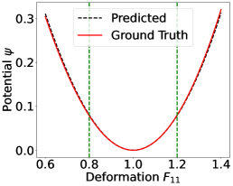
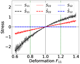
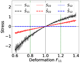
Figure 1: Fits for $L_{0}$, $L_{1}$ and $L_{2}$ (left to right) regularization. Potential $\Psi$ (upper panels, compared to noiseless data) and stress $\mathbf{S}$ (lower panels, compared to 10% noisy data). The total number of parameters for the $L_{0}$, $L_{1}$ and $L_{2}$ fits are 7, 102 and 1005, respectively.

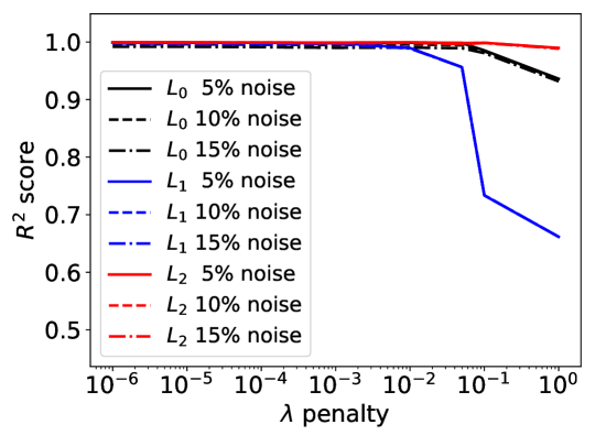
Figure 2: Comparison of the L-curves for $L_{0}$, $L_{1}$ and $L_{2}$ regularizations and increasing amounts of additive noise using the test R² score. The optimal penalty $\lambda$ depends strongly on the normalization but not as much on the added noise over the range that was studied.

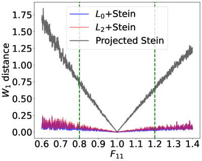
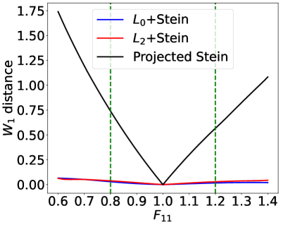
Figure 3: Comparison of Wasserstein-1 distances between the $L_{2}$+Stein, $L_{2}$+projected Stein and $L_{0}$+Stein for noisy (left, 10% heteroskedastic noise) and clean (right) data. Note the similar trends for these two cases.

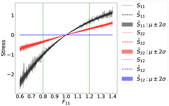
Figure 4: Comparison of mean and standard deviation predicted by $L_{0}$+Stein pushforward samples and 10 % heteroskedastic noisy validation data. Color bands indicate $\pm 2$ standard deviation from the mean, which largely overlap the noisy data.

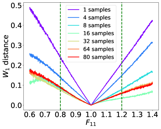
Figure 5: Convergence of Wasserstein-1 distances for $L_{0}+$Stein results and the 10 % heteroskedastic noise validation data distribution with an increasing number of data size $N_{D}$.

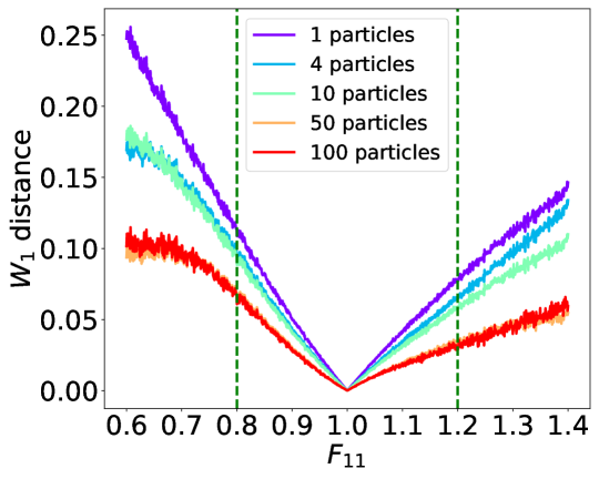
Figure 6: Convergence of Wasserstein-1 distances for $L_{0}+$Stein results and the 10 % heteroskedastic noise validation data distribution with an increasing number of particles. Note the 100 particle case overlaps the 50 particle result.

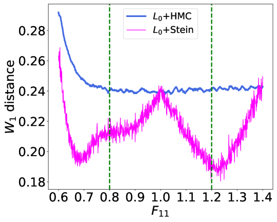
Figure 7: Comparison of Wasserstein-1 distances between the push-forward distributions obtained by SVGD and HMC, respectively and the 10% homoskedastic noise validation data.

4.2 Mechanochemistry

In phase change processes, a free energy potential $\Psi$ dependent on deformation and chemical concentration plays a central role [46, 47, 48]. In this demonstration, we take the form of the free energy from Ref.  [47]:

$$\Psi(\mathbf{E},c)= 16d_{c}c^{4}-32d_{c}c^{3}+16d_{c}c^{2}+\frac{2d_{e}}{s_{e}^{2}}\left(e_{1}^{2}+e_{6}^{2}\right)+\frac{d_{e}}{s_{e}^{4}}e_{2}^{4}+(2c-1)\frac{2d_{e}}{s_{e}^{2}}e_{2}^{2}$$ (25)

where $d_{c}=2.0$, $d_{e}=0.1$, $s_{e}=0.1$, and

$$e_{1} =\frac{1}{\sqrt{3}}\operatorname{tr}\mathbf{E}, e_{2} =\frac{1}{\sqrt{2}}(E_{11}-E_{22}), e_{6} =\sqrt{2}E_{12}, e_{3}=e_{4}=e_{5}=0$$ (26)

and $\mathbf{E}=1/2(\mathbf{C}-\mathbf{I})$ is the Lagrange strain and $c$ is the concentration. The free energy has multiple wells which are characteristic of a material that can undergo a phase change and this potential is highly nonlinear and non-convex as the projections in Fig.  8 show. Note we use a 2D, plane strain reduction of $\mathbf{E}$. Here, we enforce the normalization condition for the free energy by setting:

$$\hat{\Psi}=\hat{\Psi}^{NN}(e_{1},e_{2},e_{6},c)-\hat{\Psi}^{NN}(0,0,0,0).$$ (27)

in a manner similar to Eq.  (20). For this demonstration, we observe the stress

$$\mathbf{S}\equiv\partial_{\mathbf{E}}\Psi$$ (28)

and the chemical potential

$$\mu\equiv\partial_{c}\Psi\ .$$ (29)

for a uniform sampling of deformation space $[\mathbf{F}]_{ij}\in\delta_{ij}+\mathcal{U}[-\epsilon,\epsilon]$ with $\epsilon=0.2$ and concentration $c\in\mathcal{U}[0,1]$. The loss $\mathcal{L}$ balances the errors in the stress $\mathbf{S}$ and the chemical potential $\mu$

$$\mathcal{L}=\sum_{i}(\mathbf{S}_{i}-\hat{\mathbf{S}}(\mathbf{E}_{i},c_{i};{\bm{\theta}}))^{2}+\sum_{i}(\mu_{i}-\hat{\mu}(\mathbf{E}_{i},c_{i};{\bm{\theta}}))^{2}+\lambda\|{\bm{\theta}}\|_{p}$$ (30)

We use same path for validation as in Eq.  (22) augmented with the linear path $c=1.25(\gamma+0.4)$ with $\gamma\in[-0.4,0.4]$ through $c\in[0,1]$.

For this example, we consider a NN model with the input being the Lagrange strain and concentration, and the model predicts the free energy $\Psi$ with three hidden layers with $4,16,4$ hidden units, respectively, and softplus activations.

Fig.  9 shows that MAP fits are comparably accurate for $L_{0}$, $L_{1}$, and $L_{2}$ regularization. The models accurately predict the stress and chemical potential, as well as the free energy, which was not included in the training data. Here, the MAP model for the $L_{0}$ sparsification with $34$ parameters achieves accuracy comparable to that of the $L_{1}$ and $L_{2}$ regularized MAP models with $148$ parameters. The $L_{0}$ sparsified expression is:

$$\hat{\Psi}=2.262c-1.734e_{1}-0.357\log{\left(\frac{9.43\left(\frac{e^{9.451c}}{\left(1+e^{-0.506c}\right)^{9.855}}+1\right)^{1.085}}{\left(\frac{e^{18.73c}}{\left(1+e^{-0.506c}\right)^{7.063}}+0.019\right)^{0.728}}+1\right)}\\ -1.081\log{\left(\frac{\left(\left(1+e^{-0.506c}\right)^{5.615}e^{-20.601e_{2}}+1\right)^{0.352}e^{0.02c+0.023e_{6}}}{\left(\left(1+e^{-0.506c}\right)^{4.612}e^{18.344e_{2}}+1\right)^{0.596}}+1\right)}\\ +0.296\log{\left(9.766\left(1+e^{-7.325e_{1}}\right)^{4.219}\left(\frac{e^{18.73c}}{\left(1+e^{-0.506c}\right)^{7.063}}+0.019\right)^{0.576}\right)}\\ \left(\left(1+e^{-0.506c}\right)^{4.612}e^{18.344e_{2}}+1\right)^{5.65}\left(\left(1+e^{-0.506c}\right)^{5.615}e^{-20.601e_{2}}+1\right)^{6.124}\\ \left(e^{7.682e_{1}}+1\right)^{5.569}+1+0.485\log{\left(\frac{1890.69}{\left(\frac{e^{9.451c}}{\left(1+e^{-0.506c}\right)^{9.855}}+1\right)^{1.72}}+1\right)}-15.98$$

Fig.  10 shows how the proposed method compares to the standard, regularized techniques. The relative performance of the three methods is similar to that for the hyperelasticity demonstration, Fig.  3. Clearly, the $L_{0}$+Stein approach is superior despite using only 50 particles versus 1000 for the other two methods. Also, as shown in Table  1 the computational cost for the $L_{0}$+Stein approach is significantly lower than that of $L_{2}$+Stein approach.

	Hyperelasticity		Mechanochemistry
Method	Time [s]	Number of parameters (Deterministic)	Time [s]	Number of parameters (Deterministic)
$L_{0}$+Stein	1708	7	14862	34
$L_{2}$+Projected Stein	1794	102	5127	148
$L_{2}$+Stein	14816	1005	165052	148

Table 1: Comparison of wall clock time and number of parameters for both the deterministic optimization and the Bayesian UQ for the hyperelasticity and mechanochemistry examples. All the models were trained on a single NVIDIA RTX A6000 GPU.

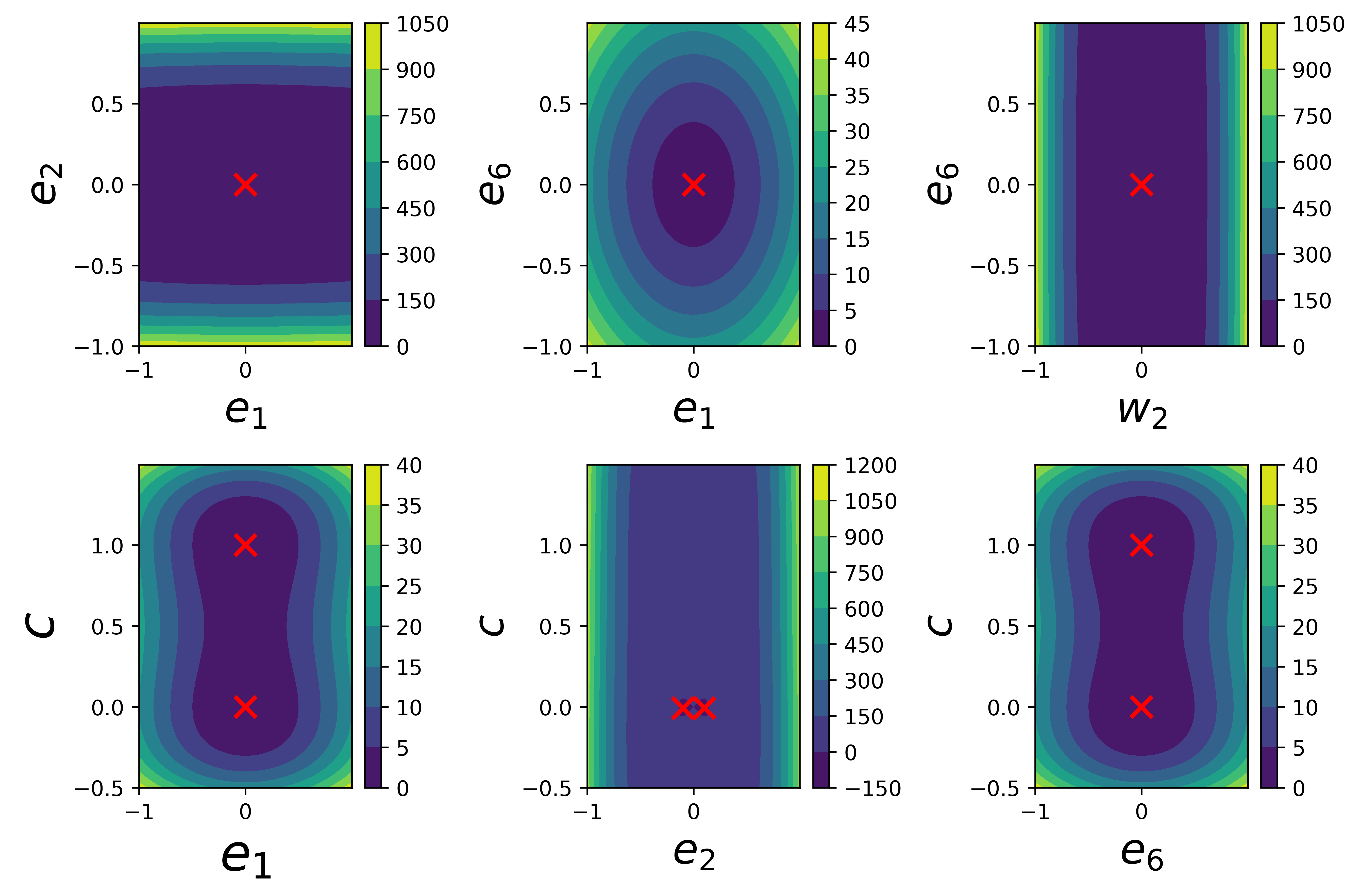
Figure 8: Free energy potential, slices through the reference configuration $\mathbf{F}=\mathbf{I}$. Red $\mathsf{X}$’s mark the location of the minima of the potential in these slices.

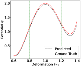
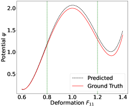
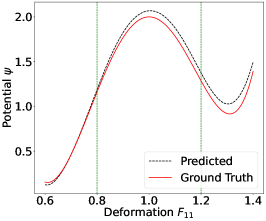
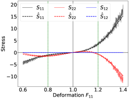
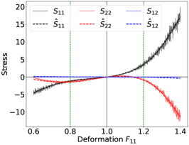
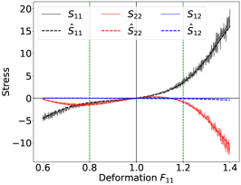
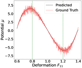
Figure 9: Fits for $L_{0}$ (left), $L_{1}$ (center), and $L_{2}$ (right) regularizations. Top row: free energy $\Psi$, middle row: stress $\mathbf{S}$, bottom row: chemical potential $\mu$. Note only stress and chemical potential are in the training data. Clearly the multiple minima of the potential are captured accurately.

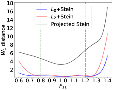
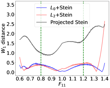
Figure 10: Comparison of Wasserstein-1 distances for $L_{0}$ sparsified Stein, $L_{2}$ regularized Stein, and $L_{2}$ regularized projected Stein for stress (left) and chemical potential (right).

5 Conclusion

For highly parameterized models like NNs, we proposed an alternative SVGD method to pSVGD that embeds more aspects of the posterior parameter manifold than linearization can provide. We demonstrated the advantages of the method on applications from mechanics. For one example we exploited the constraint of polyconvexity of the underlying potential, while the other was distinctly non-convex. For these examples, $L_{0}$ sparsification of the NN model prior to applying SVGD demonstrated superior performance to alternative regularizations and model reduction techniques.

In future work, we want to use the uncertainty information from the proposed $L_{0}$ Stein technique in forward propagation studies of large-scale finite element simulations [49, 50]. Since each Stein particle represents a model realization, this should be straightforward. In addition, we will pursue concurrent UQ and model sparsification by augmenting the Stein gradient Eq.  (14) with the gradient of a sparsifying prior. Fig.  11 demonstrates the convergence of an ensemble of particles in this augmented gradient flow with a $L_{1}$ prior. Clearly, the particles cluster around the data mean where the likelihood has high precision and are forced to zero where the likelihood precision in that parameter is low. This approach may have computational advantages when it is not feasible to find a sparse model first. Lastly, since $L_{0}$+Stein readily provides uncertainty information, it can be used in active learning based on UQ objectives such as the upper confidence bound and expected information gain [51, 52], which we wish to exploit in practical applications.

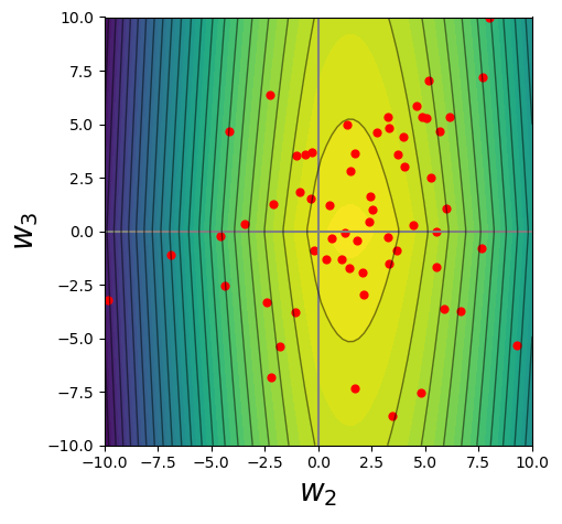
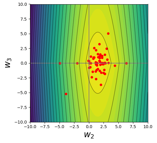
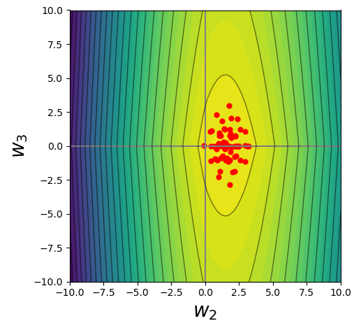
Figure 11: Demonstration of gradient descent with sparsifying prior, epoch=0 (left), 500 (middle), 1000 (right). $L_{1}$ prior and multivariate likelihood with precision $\begin{bmatrix}2&1&0\\ 1&2&0\\ 0&0&0.025\\ \end{bmatrix}$ and mean $\begin{bmatrix}1&2&3\end{bmatrix}^{T}$.

Appendix A Stein Variational Gradient Descent

Given a set of data $\mathcal{D}=\{\mathsf{x}^{i},\mathsf{y}^{i}\},_{i=1}^{N}$, with the likelihood function $\pi(\mathsf{y}|\mathsf{x},{\bm{\theta}})$ and prior $\pi({\bm{\theta}})$, as in Sec.​ 3.1, we are interested in obtaining the posterior distribution $\pi({\bm{\theta}}|\mathcal{D})$. SVGD [3] aims to approximate the posterior distribution with a variational distribution $q^{*}({\bm{\theta}})$, which lies in the restricted set of distributions $\mathcal{Q}$:

$$q^{*}({\bm{\theta}})=\underset{q\in\mathcal{Q}}{\arg\min}\,{\operatorname{KL}}(q({\bm{\theta}})\|\pi({\bm{\theta}}|\mathcal{D}))=\underset{q\in\mathcal{Q}}{\arg\min}\,\mathbb{E}_{q}[\log q({\bm{\theta}})-\log\tilde{p}({\bm{\theta}}|\mathcal{D})]\ ,$$ (31)

where $\tilde{p}({\bm{\theta}}|\mathcal{D})=\pi(\mathcal{D}|{\bm{\theta}})\pi({\bm{\theta}})=\prod_{i=1}^{N}\pi\left(\mathbf{y}^{i}|{\bm{\theta}},\mathbf{x}^{i}\right)\pi({\bm{\theta}})$ is the unnormalized posterior. The normalization constant associated with the evidence is not considered when we optimize the Kullback-Liebler (KL) divergence defined in Eq.  (31). In SVGD, we take an initial tractable distribution represented in terms of samples and then apply a transformation to each of these samples:

$$\bm{T}({\bm{\theta}})={\bm{\theta}}+\epsilon\bm{\phi}({\bm{\theta}}),$$ (32)

where $\epsilon$ is the step size and $\bm{\phi}({\bm{\theta}})\in\mathcal{F}$ is the perturbation direction within a function space $\mathcal{F}$. Therefore, $\bm{T}$ transforms the initial density $q({\bm{\theta}})$ to $q_{[\bm{T}]}({\bm{\theta}})$

$$q_{[\bm{T}]}({\bm{\theta}})=q\left(\bm{T}^{-1}({\bm{\theta}})\right)\left|\operatorname{det}\left(\nabla\bm{T}^{-1}({\bm{\theta}})\right)\right|.$$ (33)

Unlike the more common mean field variational inference, SVGD uses a particle approximation for the variational posterior rather than a parametric form. Therefore, we consider a set of samples $\{{\bm{\theta}}_{i}\}_{i=1}^{S}$, with the empirical measure:

$$\mu_{S}(d{\bm{\theta}})=\frac{1}{S}\sum_{i=1}^{S}\delta({\bm{\theta}}-{\bm{\theta}}^{i})d{\bm{\theta}}\ .$$ (34)

where $S$ is the total number of samples. While the empirical measure $\mu_{S}$ converges weakly to the true measure $\mu$ as the number of samples $S$ increases, it is important for the measure $\mu$ to weakly converge to the measure $\nu_{\pi}(\mathrm{d}{\bm{\theta}})=\pi({\bm{\theta}}\,|\,\mathcal{D})\mathrm{d}{\bm{\theta}}$ of the true posterior $p\equiv\pi({\bm{\theta}}\,|\,\mathcal{D})$. The minimum KL divergence of the variational approximation and the target distribution:

$$\min_{\bm{\phi}\in\mathcal{F}}\Big{[}\frac{\mathrm{d}}{\mathrm{d}\epsilon}\operatorname{KL}(\bm{T}\mu||\nu_{\pi})|_{\epsilon=0}\Big{]}.$$ (35)

under the transformation $\mu\to\bm{T}\mu$, determines the optimal ${\bm{\phi}}$ and approximate posterior. This term can also be expressed as [3]:

$$\frac{\mathrm{d}}{\mathrm{d}\epsilon}\operatorname{KL}(\bm{T}\mu||\nu_{\pi})|_{\epsilon=0}=-\mathbb{E}_{\mu}[\mathcal{T}_{\pi}\bm{\phi}],$$ (36)

where $\mathcal{T}_{\pi}$ is the Stein operator associated with the distribution $\pi$ given by:

$$\mathcal{T}_{\pi}\bm{\phi}=\frac{\nabla\cdot(\pi\bm{\phi})}{\pi}=\frac{(\nabla\pi)\cdot\bm{\phi}+\pi(\nabla\cdot\bm{\phi})}{\pi}=(\nabla\log\pi)\cdot\bm{\phi}+\nabla\cdot\bm{\phi}.$$ (37)

The term $\mathbb{E}_{\mu}\left[\mathcal{T}_{\pi}\bm{\phi}\right]$ evaluates the difference between the measures $\nu_{\pi}$ and $\mu$ and its maximum is defined as the Stein discrepancy $(\mathcal{S}(\mu,\pi))$:

$$\mathcal{S}(\mu,\pi)=\max_{\bm{\phi}\in\mathscr{F}}\mathbb{E}_{\mu}\left[\mathcal{T}_{\pi}\bm{\phi}\right].$$ (38)

If the functional space $\mathcal{F}$ is chosen to be the unit ball in a product reproducing kernel Hilbert space with the positive kernel $\kappa({\bm{\theta}},{\bm{\theta}}^{{}^{\prime}})$, then the Stein discrepancy has a closed-form solution [3]:

$$\bm{\phi}^{*}({\bm{\theta}})\propto\mathbb{E}_{{\bm{\theta}}^{{}^{\prime}}\sim\mu}[\mathcal{T}^{{\bm{\theta}}^{{}^{\prime}}}_{\pi}\kappa({\bm{\theta}},{\bm{\theta}}^{{}^{\prime}})]=\mathbb{E}_{{\bm{\theta}}^{{}^{\prime}}\sim\mu}[\nabla_{{\bm{\theta}}^{{}^{\prime}}}\log\pi({\bm{\theta}}^{{}^{\prime}}\,|\,\mathcal{D})\kappa({\bm{\theta}},{\bm{\theta}}^{{}^{\prime}})+\nabla_{{\bm{\theta}}^{{}^{\prime}}}\kappa({\bm{\theta}},{\bm{\theta}}^{{}^{\prime}})],$$ (39)

Appendix B Input convex neural network

In Ref.  [19], an ICNN network is defined as follows: for an output $\mathsf{y}$ an corresponding input $\mathsf{x}$, the neural network $\mathcal{N}$ with $N$ number of layers is simply:

$$\mathsf{h}_{1} = \sigma_{1}\left(\mathsf{W}_{1}\mathsf{x}+\mathsf{b}_{1}\right)$$

$$\mathsf{h}_{k} = \sigma_{k}\left(\mathsf{V}_{k}\mathsf{x}+\mathsf{W}_{k}\mathsf{h}_{k-1}+\mathsf{b}_{k}\right)\qquad k=2,\ldots,N-1$$ (40)

$$\mathsf{y} = \mathsf{V}_{N}\mathsf{x}+\mathsf{W}_{N}\mathsf{h}_{N-1}+\mathsf{b}_{N}$$

with weights $\mathsf{W}_{k}$ and $\mathsf{V}_{k}$, activation functions $\sigma_{k}$ and $1<k<N$. The weights and biases form the set of trainable parameters ${\bm{\theta}}=\{\mathsf{W}_{k},\mathsf{V}_{k},\mathsf{b}_{k}\}$. The output is convex with respect to the input if the weights $\mathsf{W}_{k}$ are non-negative and the activation functions $\sigma_{k}$ are convex and non-decreasing [19].

In this work, to be computationally efficient and to obtain faster convergence, we ignore bias terms and assign the same weight $\mathsf{V}_{k}=\mathsf{W}_{k}$ per layer for $\mathsf{V}_{k}$ while having the weight values $\mathsf{W}_{k}$ to be non-negative. Here, we consider softplus as the activation functions $\sigma_{k}$:

$$\mathsf{h}_{1} = \sigma_{1}\left(\mathsf{W}_{1}\mathsf{x}\right)$$

$$\mathsf{h}_{k} = \sigma_{k}\left(\mathsf{W}_{k}\mathsf{x}+\mathsf{W}_{k}\mathsf{h}_{k-1}\right)=\sigma_{k}\left(\mathsf{W}_{k}(\mathsf{x}+\mathsf{h}_{k-1})\right)\hskip 5.69054ptk=2,\ldots,N-1$$ (41)

$$\mathsf{y} = \mathsf{W}_{N}\mathsf{x}+\mathsf{W}_{N}\mathsf{h}_{N-1}=\mathsf{W}_{N}(\mathsf{x}+\mathsf{h}_{N-1}),$$

References

- [1] Radford M Neal and Radford M Neal. Monte Carlo implementation. Bayesian learning for neural networks, pages 55–98, 1996.
- [2] Cheng Zhang, Judith Bütepage, Hedvig Kjellström, and Stephan Mandt. Advances in variational inference. IEEE transactions on pattern analysis and machine intelligence, 41(8):2008–2026, 2018.
- [3] Qiang Liu and Dilin Wang. Stein variational gradient descent: A general purpose bayesian inference algorithm. Advances in neural information processing systems, 29, 2016.
- [4] Alex Leviyev, Joshua Chen, Yifei Wang, Omar Ghattas, and Aaron Zimmerman. A stochastic stein variational newton method. arXiv preprint arXiv:2204.09039, 2022.
- [5] Peng Chen, Keyi Wu, Joshua Chen, Tom O’Leary-Roseberry, and Omar Ghattas. Projected stein variational newton: A fast and scalable bayesian inference method in high dimensions. Advances in Neural Information Processing Systems, 32, 2019.
- [6] Peng Chen and Omar Ghattas. Projected stein variational gradient descent. Advances in Neural Information Processing Systems, 33:1947–1958, 2020.
- [7] Michael Betancourt. A conceptual introduction to Hamiltonian Monte Carlo. arXiv preprint arXiv:1701.02434, 2017.
- [8] Richard Kurle, Ralf Herbrich, Tim Januschowski, Yuyang Bernie Wang, and Jan Gasthaus. On the detrimental effect of invariances in the likelihood for variational inference. Advances in Neural Information Processing Systems, 35:4531–4542, 2022.
- [9] Jeremias Knoblauch, Jack Jewson, and Theodoros Damoulas. An optimization-centric view on bayes’ rule: Reviewing and generalizing variational inference. The Journal of Machine Learning Research, 23(1):5789–5897, 2022.
- [10] Christos Louizos, Max Welling, and Diederik P Kingma. Learning sparse neural networks through regularization. arXiv preprint arXiv:1712.01312, 2017.
- [11] David M Blei, Alp Kucukelbir, and Jon D McAuliffe. Variational inference: A review for statisticians. Journal of the American statistical Association, 112(518):859–877, 2017.
- [12] Qiang Liu and Dilin Wang. Stein variational gradient descent as moment matching. Advances in Neural Information Processing Systems, 31, 2018.
- [13] Christopher M Bishop and Nasser M Nasrabadi. Pattern recognition and machine learning, volume 4. Springer, 2006.
- [14] Ian Goodfellow, Yoshua Bengio, and Aaron Courville. Deep learning. MIT press, 2016.
- [15] Peter M Williams. Bayesian regularization and pruning using a laplace prior. Neural computation, 7(1):117–143, 1995.
- [16] Christos Louizos, Karen Ullrich, and Max Welling. Bayesian compression for deep learning. Advances in neural information processing systems, 30, 2017.
- [17] Jan Niklas Fuhg, Reese Edward Jones, and Nikolaos Bouklas. Extreme sparsification of physics-augmented neural networks for interpretable model discovery in mechanics. Computer Methods in Applied Mechanics and Engineering, 426:116973, 2024.
- [18] Mart Van Baalen, Christos Louizos, Markus Nagel, Rana Ali Amjad, Ying Wang, Tijmen Blankevoort, and Max Welling. Bayesian bits: Unifying quantization and pruning. Advances in neural information processing systems, 33:5741–5752, 2020.
- [19] Brandon Amos, Lei Xu, and J Zico Kolter. Input convex neural networks. In International Conference on Machine Learning, pages 146–155. PMLR, 2017.
- [20] Vahidullah Tac, Francisco Sahli Costabal, and Adrian B Tepole. Data-driven tissue mechanics with polyconvex neural ordinary differential equations. Computer Methods in Applied Mechanics and Engineering, 398:115248, 2022.
- [21] Peiyi Chen and Johann Guilleminot. Polyconvex neural networks for hyperelastic constitutive models: A rectification approach. Mechanics Research Communications, 125:103993, 2022.
- [22] Faisal As’ad, Philip Avery, and Charbel Farhat. A mechanics-informed artificial neural network approach in data-driven constitutive modeling. International Journal for Numerical Methods in Engineering, 123(12):2738–2759, 2022.
- [23] Kailai Xu, Daniel Z Huang, and Eric Darve. Learning constitutive relations using symmetric positive definite neural networks. Journal of Computational Physics, 428:110072, 2021.
- [24] Dominik K Klein, Mauricio Fernández, Robert J Martin, Patrizio Neff, and Oliver Weeger. Polyconvex anisotropic hyperelasticity with neural networks. Journal of the Mechanics and Physics of Solids, 159:104703, 2022.
- [25] Dominik K Klein, Fabian J Roth, Iman Valizadeh, and Oliver Weeger. Parametrized polyconvex hyperelasticity with physics-augmented neural networks. Data-Centric Engineering, 4:e25, 2023.
- [26] Karl A Kalina, Philipp Gebhart, Jörg Brummund, Lennart Linden, WaiChing Sun, and Markus Kästner. Neural network-based multiscale modeling of finite strain magneto-elasticity with relaxed convexity criteria. Computer Methods in Applied Mechanics and Engineering, 421:116739, 2024.
- [27] Jan N Fuhg, Nikolaos Bouklas, and Reese E Jones. Learning hyperelastic anisotropy from data via a tensor basis neural network. Journal of the Mechanics and Physics of Solids, 168:105022, 2022.
- [28] Jan N Fuhg, Lloyd van Wees, Mark Obstalecki, Paul Shade, Nikolaos Bouklas, and Matthew Kasemer. Machine-learning convex and texture-dependent macroscopic yield from crystal plasticity simulations. Materialia, 23:101446, 2022.
- [29] Jan Niklas Fuhg, Craig M Hamel, Kyle Johnson, Reese Jones, and Nikolaos Bouklas. Modular machine learning-based elastoplasticity: Generalization in the context of limited data. Computer Methods in Applied Mechanics and Engineering, 407:115930, 2023.
- [30] Julia Ling, Reese Jones, and Jeremy Templeton. Machine learning strategies for systems with invariance properties. Journal of Computational Physics, 318:22–35, 2016.
- [31] Nathaniel Thomas, Tess Smidt, Steven Kearnes, Lusann Yang, Li Li, Kai Kohlhoff, and Patrick Riley. Tensor field networks: Rotation-and translation-equivariant neural networks for 3d point clouds. arXiv preprint arXiv:1802.08219, 2018.
- [32] Roger Ghanem, David Higdon, Houman Owhadi, et al. Handbook of uncertainty quantification, volume 6. Springer New York, 2017.
- [33] Harald Steck and Tommi Jaakkola. On the dirichlet prior and bayesian regularization. Advances in neural information processing systems, 15, 2002.
- [34] Daniela Calvetti and Erkki Somersalo. Inverse problems: From regularization to bayesian inference. Wiley Interdisciplinary Reviews: Computational Statistics, 10(3):e1427, 2018.
- [35] Qiang Liu. Stein variational gradient descent as gradient flow. Advances in neural information processing systems, 30, 2017.
- [36] Diederik P Kingma and Jimmy Ba. Adam: A method for stochastic optimization. arXiv preprint arXiv:1412.6980, 2014.
- [37] Marc C Kennedy and Anthony O’Hagan. Bayesian calibration of computer models. Journal of the Royal Statistical Society: Series B (Statistical Methodology), 63(3):425–464, 2001.
- [38] John M Ball. Convexity conditions and existence theorems in nonlinear elasticity. Archive for rational mechanics and Analysis, 63:337–403, 1976.
- [39] Miroslav Silhavy. The mechanics and thermodynamics of continuous media. Springer Science & Business Media, 2013.
- [40] Frank Rosenblatt. Principles of neurodynamics. perceptrons and the theory of brain mechanisms. Technical report, Cornell Aeronautical Lab Inc., Buffalo NY, 1961.
- [41] Jan N Fuhg, Reese E Jones, and Nikolaos Bouklas. Extreme sparsification of physics-augmented neural networks for interpretable model discovery in mechanics. arXiv preprint arXiv:2310.03652, 2023.
- [42] Raymond W Ogden, Giuseppe Saccomandi, and Ivonne Sgura. Fitting hyperelastic models to experimental data. Computational Mechanics, 34:484–502, 2004.
- [43] Cornelius O Horgan. The remarkable gent constitutive model for hyperelastic materials. International Journal of Non-Linear Mechanics, 68:9–16, 2015.
- [44] Jan Fuhg, Nikolaos Bouklas, and Reese Jones. Stress representations for tensor basis neural networks: alternative formulations to finger-rivlin-ericksen. Journal of Computing and Information Science in Engineering, pages 1–39, 2024.
- [45] Heinz W Engl and Wilhelm Grever. Using the l–curve for determining optimal regularization parameters. Numerische Mathematik, 69(1):25–31, 1994.
- [46] Krishna Garikipati. Perspectives on the mathematics of biological patterning and morphogenesis. Journal of the Mechanics and Physics of Solids, 99:192–210, 2017.
- [47] Shiva Rudraraju, Anton Van der Ven, and Krishna Garikipati. Mechanochemical spinodal decomposition: a phenomenological theory of phase transformations in multi-component, crystalline solids. npj Computational Materials, 2(1):1–9, 2016.
- [48] GH Teichert, S Das, M Faghih Shojaei, J Holber, T Mueller, L Hung, V Gavini, and K Garikipati. Bridging scales with machine learning: From first principles statistical mechanics to continuum phase field computations to study order disorder transitions in lixcoo2. arXiv preprint arXiv:2302.08991, 2023.
- [49] Reese E Jones, Michael T Redle, Hemanth Kolla, and Julia A Plews. A minimally invasive, efficient method for propagation of full-field uncertainty in solid dynamics. International Journal for Numerical Methods in Engineering, 122(23):6955–6983, 2021.
- [50] Saibal De, Reese E Jones, and Hemanth Kolla. Accurate data-driven surrogates of dynamical systems for forward propagation of uncertainty. arXiv preprint arXiv:2310.10831, 2023.
- [51] Mingkun Li and Ishwar K Sethi. Confidence-based active learning. IEEE transactions on pattern analysis and machine intelligence, 28(8):1251–1261, 2006.
- [52] Burr Settles. From theories to queries: Active learning in practice. In Active learning and experimental design workshop in conjunction with AISTATS 2010, pages 1–18. JMLR Workshop and Conference Proceedings, 2011.