Improved Graph- based semi-supervised learning Schemes

Abstract.

In this work, we improve the accuracy of several known algorithms to address the classification of large datasets when few labels are available. Our framework lies in the realm of graph-based semi-supervised learning. With novel modifications on Gaussian Random Fields Learning and Poisson Learning algorithms, we increase the accuracy and create more robust algorithms. Experimental results demonstrate the efficiency and superiority of the proposed methods over conventional graph-based semi-supervised techniques, especially in the context of imbalanced datasets.

1. Introduction

In this paper, we consider semi-supervised learning approaches for classifying many unlabeled data when very few labels are given. Our objective is to refine existing classification algorithms to perform effectively in the cases with limited labeled data. We introduce innovative modifications to established algorithms to enhance accuracy and robustness.

When there is an insufficient amount of labeled data available, models may struggle to learn effectively and to predict accurately. One way to improve this is by incorporating lots of unlabeled data along with those few labeled samples. This approach helps the model to learn about the structure of data, enhancing its performance especially when there aren’t many examples to learn from. Considering mentioned advantage, semi-supervised learning has received much attention in the past few decades [18, 11, 17, 22]. A common approach for doing this is graph-based semi-supervised learning. We use graphs to show how different samples of data are connected, helping to understand both labeled and unlabeled data better. We refer to recent surveys [19, 12] as a comprehensive review of existing algorithms on graph-based learning.

Although existing semi-supervised algorithms show good performance on balanced data, they frequently struggle in complex real-world applications, particularly with highly imbalanced datasets. One of the issues is overfilling to the limited labeled data available and not making full use of the structural information present in the unlabeled data. The Imbalance Ratio (IR) is an important factor and represents the ratio of samples in each of Minority and Majority classes. The bigger IR, the more difficult the problem becomes, to see more about techniques to handle imbalanced data see [20]. Our objective is to introduce innovative modifications to established algorithms, enhancing both accuracy and robustness against these challenges.

A common approach to use unlabeled data in semi-supervised learning is to build a graph over the data. This means geometric or topological properties of the unlabeled data have been used to improve algorithms. In [13] a general framework for constructing a graph is proposed and they named it Graph-based Semi-supervised Learning via Improving the Quality of the Graph Dynamically.

First, we construct a weight matrix $W$ or similarity matrix over the data set, which encodes the similarities between pairs of data nodes. If our data set consists of $n$ points ${\mathcal{X}}=\{x_{1},x_{2},\cdots,x_{n}\}\subset\mathbb{R}^{d}$, then the weight matrix $W$ is an $n\times n$ symmetric matrix, where the element $w_{ij}$ represents the similarity between two data points $x_{i}$ and $x_{j}$. When constructing a KNN graph, the weight between node $x_{i}$ and node $x_{j}$ typically depends on the distance or similarity between the nodes. A common choice for the weight function is the Gaussian kernel or the inverse of the distance between nodes.

The similarity is always nonnegative and should be large when $x_{i}$ and $x_{j}$ are close together spatially, and small (or zero), when $x_{i}$ and $x_{j}$ are far apart. Subsequently, by leveraging information from the constructed graph, labels are propagated from the given labeled instances to the unlabeled data.

The main contribution of the current work is as follows.

• Modified GRF and Improved GRF Learning Algorithms: To speed up convergence and handle imbalances more effectively by incorporating the stationary distribution $\pi$ of the random walk on the graph.

• Improved Poisson Learning Algorithm: Introduces regularization terms to enhance performance on imbalanced data.

2. Problem setting and previous works

This section is devoted as an introduction to PDEs on graph and setting our problem. Let ${\mathcal{X}}=\{x_{1},\cdots,x_{n}\}$ denote the vertices of a graph with symmetric edge weight $w_{ij}$ between $x_{i},x_{j}\in{\mathcal{X}}$ and let $W=[w_{ij}]$. We assume there is a subset of the nodes ${\mathcal{X}}_{l}={\{x_{1},\cdots,x_{l}}\}\subset{\mathcal{X}}$ for which labels are provided by a labeling function $g:{\mathcal{X}}_{l}\rightarrow{\mathbb{R}}^{k}$, forming our training set $(x_{i},y_{i})_{i=1}^{l}$. The degree of a vertex $x_{i}$ is given by $d_{i}=\sum_{j}w_{ij}$ and let $d=\sum_{i}d_{i}$. Matrix $D$ denotes the diagonal matrix which has $d_{i}$ on main the diagonal.

Let $\ell^{2}({\mathcal{X}})$ denote the set of functions $u:{\mathcal{X}}\rightarrow\mathbb{R}$ equipped with the inner product

$$(u,v)=\sum\limits_{x\in{\mathcal{X}}}u(x)v(x),$$

for functions $u,v:{\mathcal{X}}\rightarrow\mathbb{R}$. We also define a vector field on the graph to be an antisymmetric function $V:{\mathcal{X}}\times{\mathcal{X}}\rightarrow\mathbb{R}^{2}$, i.e. $V(x,y)=-V(y,x)$ and denote the space of all vector fields by $\ell^{2}({\mathcal{X}}^{2})$.

The gradient of a function $u\in\ell^{2}({\mathcal{X}})$ is the vector field

$$\nabla u(x,y)=u(y)-u(x).$$

The unnormalized graph laplacian ${\mathcal{L}}$ of a function $u\in\ell^{2}({\mathcal{X}})$ is defined as

$${\mathcal{L}}u(x):=-{\rm div\,}(\nabla u)(x)=\sum_{y\in{\mathcal{X}}}w_{xy}(u(x)-u(y)).$$

Most graph-based semi-supervised learning aims to find a function on the graph that closely matches the given labels while also maintaining smoothness. It is shown in [23] that the graph Laplacian regularization is effective because it forces the labels to be consistent with the graph structure.

To model label propagation in semi-supervised learning, it is assumed that the learned labels vary smoothly and do not change rapidly within high-density regions of the graph (smoothness assumptions) [4]. Based on this assumption different approaches have been proposed, we refer to the pioneer methods Laplace learning, [21] see also [3, 4].

Let $U$ stand for the label matrix $U$ that shows the class information of each element. A general form of a graph-based semi-supervised learning for data classification can be formulated as a minimization of an energy:

$$R(U)+\mu F(U),$$

where $R(U)$ is a regularization term incorporating the graph weights, and $F(U)$ is a forcing term, which usually incorporates the labeled points and their class information.

In Laplace learning algorithm the labels are extended by finding the minimizer $U:{\mathcal{X}}\rightarrow\mathbb{R}^{k}$ for the following problem

(1) $$\begin{cases}&\min J_{n}(U):=\frac{1}{2}\sum\limits_{i=1}^{n}\sum\limits_{j=1}^{n}w_{ij}|U(x_{i})-U(x_{j})|^{2}\\ &\text{subject to }U(x_{i})=y_{i},\quad\text{ for }i=1,2,\cdots,l.\end{cases}$$

The minimizer will be a harmonic function satisfying

$$\left\{\begin{array}[]{ll}{\mathcal{L}}U(x)=0,&x\in{\mathcal{X}}\setminus{\mathcal{X}}_{l},\\ U=g,&\text{ on }{\mathcal{X}}_{l},\\ \end{array}\right.$$

where ${\mathcal{L}}$ is the unnormalized graph Laplacian given by

$$\mathcal{L}U(x_{i})=\sum\limits_{j=1}^{n}w_{ij}\,(U(x_{i})-U(x_{j})).$$

Let $U=(u_{1},\cdots,u_{k})$ be a solution of (1), the label of node $x_{i}\in{\mathcal{X}}\setminus{\mathcal{X}}_{l}$ is dictated by

$$\underset{j\in{\{1,\cdots,k}\}}{\textrm{arg max}}{u_{j}(x_{i})}.$$

This means that Laplace learning uses harmonic extension on a graph to propagate labels. If the number of labeled data samples is finite while the number of unlabeled data tends to infinity, then Laplace learning becomes degenerate and the solutions become roughly constant with a spike at each labeled data point.

Later it has been observed that the Laplace learning can give poor results in classification [15]. The results are often poor because the solutions have localized spikes near the labeled points, while being almost constant far from them. To overcome this problem several versions of the Laplace learning algorithm have been proposed, for instance, Laplacian regularization, [2], weighted Laplacian, [10] and $p$-Laplace learning, [8, 16]. Also, the limiting case in $p$-Laplacian when $p$ tends to infinity is so-called Lipschitz learning is studied in [14] and similar to continuum PDEs is related to finding the absolute minimal Lipschitz extension of the training data. Recently, in [7] another approach to increase accuracy of Laplace learning is given and called Poisson learning.

In [9] the authors consider the case that the number of labeled data points grows to infinity also when the total number of data points grows. Let $\beta$ denote the labeling rate. They show that for a random geometric graph with length scale $\varepsilon$ if $\beta\geq\varepsilon^{2}$, then the solution becomes degenerate and spikes occurs, while for the case $\beta\leq\varepsilon^{2}$, Laplacian learning is well-posed and consistent with a continuum Laplace equation.

The authors in [7] have proposed a scheme, called Poisson learning that replaces the label values at training points as sources and sinks, and solves the Poisson equation on the graph as follows:

(2) $$\left\{\begin{array}[]{ll}\mathcal{L}\mathbf{u}(x_{i})=y_{i}-\overline{y}&1\leq i\leq l,\\ \mathcal{L}\mathbf{u}(x_{i})=0&l+1\leq i\leq n,\\ \end{array}\right.$$

with further condition $\sum_{i=1}^{n}d(x_{i})\mathbf{u}(x_{i})=0$, where $\overline{y}=\frac{1}{l}\sum_{i=1}^{l}y_{i}$ is the average label vector. In the next section, we review this scheme in detail and will consider some modification to this algorithm.

In [6, 5] a graph-based semi-supervised learning scheme based on the theory of the spatial segregation of competitive systems, is given. The scheme is based on the minimizing (1) with constraint

$$u_{i}(x)\cdot u_{j}(x)=0,\qquad\text{ for all }x\in{\mathcal{X}},\;1\leq i\neq j\leq k.$$

3. Proposed Algorithms

3.1. Modified Gaussian Random Fields (MGRF)

Let, as before ${\mathcal{X}}={\{x_{1},\cdots,x_{n}}\}$ denote the data points or vertices in a graph. We assume there is a subset of the nodes ${\mathcal{X}}_{l}={\{x_{1},\cdots,x_{l}}\}\subset{\mathcal{X}}$ that their labels are given with a label function $g:{\mathcal{X}}_{l}\rightarrow{\mathbb{R}}^{k}$. It is further assumed that $y_{i}=g(x_{i})\in\{e_{1},\cdots,e_{k}\}$ where $e_{i}$ is the standard basis in $\mathbb{R}^{k}$ and represents the $i\textsuperscript{th}$ class. In graph-based semi-supervised learning, we aim to extend labels to the rest of the vertices ${\mathcal{X}}_{u}=\{x_{l+1},\cdots,x_{n}\}$.

The scheme described below is known as Gaussian Random Fields (GRF) [21]. For any matrix $U=(U_{ij})\in\mathbb{R}^{n\times k}$, $U_{i\cdot}$ represents the $i^{\text{th}}$ row of $U$. They consider the following minimization problem

(3) $$\underset{U_{l\cdot}=Y_{l\cdot}}{\text{arg min}}\,Tr(U^{T}LU),\quad U\in\mathbb{R}^{n\times k}$$

Here $L=D-W$. Let us split the weight matrix $W$ into four blocks as

$$\mathbf{W}=\left(\begin{array}[]{cc}W_{ll}&W_{lu}\\ W_{ul}&W_{uu}\\ \end{array}\right).$$

Also let $P=D^{-1}W$ and decompose $P$ and $U$ to $U_{l}$ and $U_{u}$, then the solution of minimization problem (3) is given by:

(4) $$U_{u}=(I-P_{uu})^{-1}P_{ul}U_{l}.$$

The following iterative scheme was proposed in [21].

(5) $$U^{(m+1)}=\alpha SU^{(m)}+(1-\alpha)Y,$$

where $S=D^{\frac{-1}{2}}WD^{\frac{-1}{2}}$ and $Y$ denotes the vector of initial labels.

We modify the scheme (5) to achieve better accuracy. In scheme (5), $U^{(m)}$ is a vector where the sign of the $i^{\textrm{th}}$ element of $U^{m}$ indicates the class of $x_{i}$. For a sample $x_{i}\in{\mathcal{X}}_{l}$ its label belongs ${\{\pm 1}\}$.

Let $l_{1},l_{2}$ denote the number of labels in Class 1 and Class 2, respectively with $l=1_{1}+l_{2}$. Then the vector $B\in\mathbb{R}^{n}$ is defined as follows

$$B=\left\{\begin{array}[]{ll}\frac{l_{2}}{l},&x_{i}\in{\mathcal{X}}_{l}\,\textrm{and}\,y_{i}=1,\\ \frac{-l_{1}}{l},&x_{i}\in{\mathcal{X}}_{l}\,\textrm{and}\,y_{i}=-1,\\ 0&x_{i}\in{\mathcal{X}}\setminus{\mathcal{X}}_{l}.\\ \end{array}\right.$$

Algorithm 1, named ”MGRF”, extends the GRF scheme by modifying the initial labels vector $Y$ and iterating over all nodes.

Algorithm 1 (MGRF)

Input:Matrix $W$, initial label $Y$, parameter $\alpha$, tolerance $\varepsilon$.
Output: Label $y_{i}$ for each point $x_{i}$ or equivalently $U\in\mathbb{R}^{n}$

• Calculate matrices: $D$, $S$ and $B$

• Initialize $U^{0}=D^{-1}Y$

• while $\|U^{(m+1)}-U^{(m)}\|>\varepsilon$ do

• $U^{(m+1)}=\alpha SU^{(m)}+(1-\alpha)D^{\frac{-1}{2}}B^{T}$

• end while

• Assign each point $x_{i}$ the sign of $U^{*}_{i}$
  

• $U^{*}=\underset{m\rightarrow\infty}{Lim}U^{m}.$

Next, we explain how to improve the efficiency of the scheme MGRF. Let $\pi$ be the unique stationary distribution of the random walk on the graph represented by the normalized affinity matrix $S$, then $\pi$ satisfies the equation:

$$\pi S=\pi,$$

$\pi$ is a row vector representing the stationary distribution.

Consider matrix $G$, where all rows of $G$ are equal and composed of $\pi$. By subtracting $G$ from $S$ in each iteration, we effectively bias the random walk towards the stationary distribution consequently, accelerates the convergence towards the stationary distribution of the graph. This strategy makes the algorithm robust to initial conditions and parameter choices. Furthermore, it prevents the dominance of majority classes, thus improving the overall classification performance, particularly in imbalanced data sets.

The details of the scheme are given in algorithm 2 which we call it Improved Gaussian Random Fields (IGRF).

Algorithm 2 (IGRF)

Input:Matrix $W$, $Y$, parameters $\alpha_{1},\alpha_{2},\alpha_{3},$ tolerance $\varepsilon$
Output: Label $y_{i}$ for each point $x_{i}$ or equivalently $U\in\mathbb{R}^{n}$

• Calculate matrices: $S$, $B$ and $\pi$

• Initialize $U^{0}=D^{-1}Y$

• while $\|U^{(m+1)}-U^{(m)}\|>\varepsilon$ do

• $U^{(m+1)}=(\alpha_{1}S-\alpha_{2}G+\alpha_{3}I)U^{(m)}+(1-\alpha_{1})D^{\frac{-1}{2}}B^{T}$

• end while

• Assign each point $x_{i}$ the sign of $U^{*}_{i}$
  

• $U^{*}=\underset{m\rightarrow\infty}{Lim}U^{m}.$

3.2. Improved Poisson Learning(IPL)

In this section, we aim to improve the efficiency of Poisson Learning given by Algorithm 3 (see [7]). Let $b\in\mathbb{R}^{k}$ be the vector whose $i^{\textrm{th}}$ entry $b_{i}$ is the fraction of data points belonging to class $i$.

Algorithm 3 Poisson Learning

Input: ${\mathcal{X}},W$, $Y\in\mathbb{R}^{k\times l}$ (given labels), $b$, $T$:(number of iterations)
Output:$U\in\mathbb{R}^{n\times k}$ predicted class labels, and classification results

• $D\leftarrow W\mathds{1}$

• $L\leftarrow D-W$

• $\overline{y}\leftarrow\frac{1}{l}Y\mathds{1}$

• $B\leftarrow[Y-\overline{y},zeros(k,n-l)]$

• $U\leftarrow\textrm{zeros}(n,k)$

• For $m=1:T$ do

• $U^{(m)}=U^{(m-1)}+D^{-1}(B^{T}-LU^{m-1})$

• end for

• $U^{m}=U^{m}\cdot\text{diag}(b/\bar{y})$.

The main step of the Poisson Algorithm can be rewritten as

(6) $$\begin{split}U^{(m)}&=U^{(m-1)}+D^{-1}(B^{T}-(D-W)U^{(m-1)})\\ &=U^{(m-1)}+D^{-1}B^{T}-U^{(m-1)}+D^{-1}WU^{(m-1)}),\\ &=PU^{(m-1)}+D^{-1}B^{T}\end{split}$$

where $P=D^{-1}W.$ Choosing $U^{0}=D^{-1}B^{T}$ then (6) implies

$$U^{(m)}=\left(\sum_{i=0}^{m-1}P^{i}\right)D^{-1}B^{T}.$$

Next, we determine the limit of $P^{m}$ as $m$ tends to infinity. From Markov chains theory, for an irreducible and aperiodic Markov chain, $P^{m}$ converges to a matrix where all rows are identical and represent the stationary distribution of the Markov chain. It represents the long-term relative frequencies of being in each state of the Markov chain.

This stationary distribution can be computed by finding the left eigenvector corresponding to the eigenvalue one of the transition matrix $P$, i.e,

$$\pi P=\pi.$$

It is handy to verify that $\pi=(\frac{d_{1}}{d},\frac{d_{2}}{d}\cdots,\frac{d_{n}}{d}).$ We make ansatz that the limit of matrix $P$ is $Q$ with matrix $Q$ being rank one matrix with rows $\pi$. Thus

$$\underset{m\rightarrow\infty}{Lim}P^{m}=\underset{m\rightarrow\infty}{Lim}P^{m-1}P=QP=Q.$$

It worths to see $P$ has an eigenvalue equal $one,$ means $I-P$ is not invertible means one can not extract the fixed point for iterative scheme given by (6). This shows the sequence in (6) is not convergent.

Our change in the Poisson algorithm is to subtract matrix $Q$ from $P$. Our iterative scheme is as follows

$$U^{(m+1)}=(P-Q)U^{m}+D^{-1}B^{T}.$$

Keeping in mind the facts $QP=Q$, and $Q^{J}=Q(J=1,2,\cdots$) then it is easy to check

$$\underset{m\rightarrow\infty}{\text{lim}}\,(P-Q)^{m}=0.$$

Moreover, with a slightly change, our iterative scheme called Improved Poisson Learning is

(7) $$U^{(m+1)}=(P-\alpha_{1}Q)U^{m}+\alpha_{2}D^{-1}B^{T},$$

where parameters $0<\alpha_{1}\leq 1$ and $\alpha_{2}>0$.

The scheme updates the label matrix $U$ using a combination of transition probabilities, regularization terms, and initial label information. It converges faster as it focuses entirely on the graph’s intrinsic structure and connectivity. Furthermore, we might add the term $\alpha I$ to iterative scheme (7).

Algorithm 4 (IPL)

Input:Matrix $W$, initial label matrix $Y$, parameters $\alpha_{1},\alpha_{2},\alpha_{3}$.
Output:Label $y_{i}$ for each point $x_{i}$ or equivalently $U\in\mathbb{R}^{n\times k}$

• Calculate matrices: $D$ transition matrix $P$, $Q$

• Initialize $U^{0}=D^{-1}Y$

• while not convergent do

• $U^{(m+1)}=(P-\alpha_{1}Q+\alpha_{2}I)U^{m}+\alpha_{3}D^{-1}B^{T}$

• end while

• Assign each point $x_{i}$ class $y_{i}=\underset{j}{\text{arg max}}\,U^{*}$ where
  

• $U^{*}=\underset{m\rightarrow\infty}{Lim}U^{m}$

Adding $\alpha_{2}I$ to the transition matrix $P$ effectively increases the self-transition probabilities of nodes in the graph by $\alpha_{2}$. This can be interpreted as giving more weight to the existing labels in the updating process. It may help stabilize the iterative process by ensuring that each node retains some influence from its current label in the next iteration. The addition of $\alpha_{2}I$ can also help prevent numerical instability issues, particularly since $P$ and $Q$ have eigenvalues close to one.

4. Experimental results

In this section, we compare the proposed algorithms with some existing semi-supervised learning algorithms. For imbalanced data, we use evaluation metrics that are robust, such as precision, recall, and ${\rm F}_{1}$-score. These metrics provide a more comprehensive assessment of model performance on imbalanced data compared to accuracy.

For simplicity reason, we name the minor class as positive class interchangeably. Precision measures the accuracy of the positive predictions. It is the ratio of true positive predictions to the total predicted positives. Recall measures the ability to capture all positive samples. It is the ratio of true positive predictions to the total actual positives. $F_{1}$ Score is the harmonic mean of precision and recall. It balances the two metrics, especially useful in the case of imbalanced data sets. The term of $F_{1}$ score for each class is defined as follows:

(8) $${\rm F}_{1}(j)=2\times\dfrac{{\rm{Recall}}(j)\times{\rm{Precision}}(j)}{{\rm{Recall}}(j)+{\rm{Precision}}(j)}\quad j=1,2.$$

Accuracy measures the overall correctness of the model. It is the ratio of all correct predictions to the total number of samples.

Example 4.1.

We consider balanced Two-Moon pattern, we generate a set of 1000 points, with noise level $0.15$. Increasing noise will make classes more overlapping. In Algorithm IPL, the parameters are set as $\alpha_{1}=0.001,\alpha_{2}=0.02,\alpha_{3}=1$.

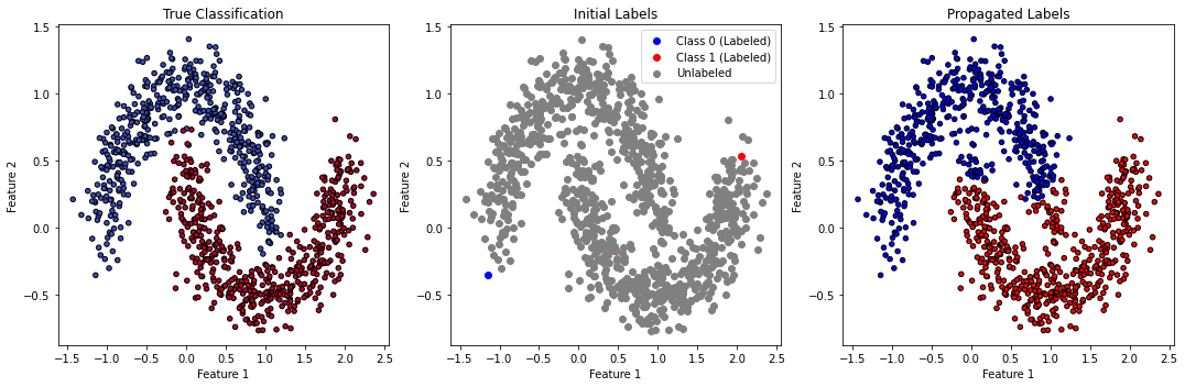
Figure 1. The classification on Two-Moon.

In Table 1, we present a comparison between Algorithms IGRF and IPL, utilizing the two moons dataset consisting of $n=1000$ points with a noise level set at $0.15$.

For Algorithm IGRF, we construct the affinity matrix using the RBF (Gaussian) kernel, which offers a smoother affinity measure than the $k$-nearest neighbors graph. The parameters of IGRF are set as $\alpha_{1}=.99,\alpha_{2}=0.005,\alpha_{3}=0.05.$

In the IPL algorithm, we employ a grid search over hyperparameters to determine the optimal parameters for various numbers of initial labels. However, this process is time-consuming. The table displays the average accuracy for each number of initial labels per class.

Table 1. Two moon, balanced case

Average overall accuracy over 100 trials for two moon
number of labels per class	1	2	3	4	5
IGRF	94.64	97.15	98.05	98.348	98.53
IPL	86.30	89.55	91.86	92.12	93.04
Poisson	83.23	87.985	90.406	91.953	92.70

Example 4.2.

Next, we generate imbalance two half moons with 950 samples from Majority class and 50 samples from Minority. We implement the IGRF scheme with two labeled points per classes. The average of accuracy over 100 runs is $96.765$. Also we compute the average of the Confusion Matrix over 100 runs.

$$\left(\begin{array}[]{cc}30.27&19.73\\ 11.62&938.38\\ \end{array}\right).$$

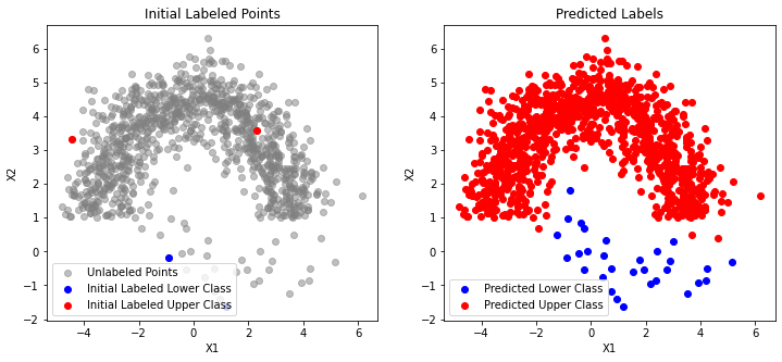
Figure 2. The classification on Imbalanced Two-Moons.

Example 4.3.

In this example, we implement Algorithm 1 (MGRF) and analyze a scenario where the data points are distributed across two circles. The configuration is set as follows: the major class contains 1,000 samples,while the minor class contains 100; noise level is set at 0.1; the maximum number of iterations is 1,500; the tolerance is set at $=10^{-8}$, $\alpha=.985$ and there are 3 labeled samples per class. Refer to Figure 3 for more details. The average confusion matrix, calculated over 100 trials, is presented below. Figure 3 also displays the initial labeled points and the predictions made by the MGRF algorithm.

$$\left(\begin{array}[]{cc}919.72&80.28\\ 25.47&74.53\\ \end{array}\right).$$

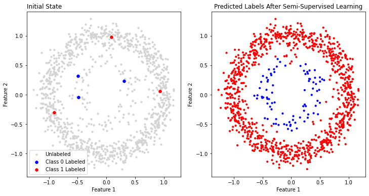
Figure 3. The classification on (two-circles ).

Example 4.4.

Table 2 describes the accuracy $(\%)$ of IPL algorithm compared to Poisson and Segregation algorithms, on Cifar-10 data set with 3 classes and 4500 nodes (1500 nodes per class) with several labels per class. The results are averages over 100 trials, which demonstrates superior performance of our scheme IPL for different label rates.

Table 2. Cifar-10 data set

Average accuracy over 30 trials for 3 classes on Cifar-10 dataset
number of labels	2	3	4	5	10	20	40
Poisson	37.5	39.5	40.3	41.4	44.10	48.7	50.3
Segregation	34.9	35.6	36.2	38.6	42.4	45.3	47.7
IPL	45.226	46.546	47.382	48.341	53.152	54.966	57.031

Dimensionality reduction techniques like PCA or feature transformations provide better feature separation for the proposed algorithms, however, we did not involve PCA in algorithm. We just used PCA, in Figure 4 to plot the classification for 3 classes on the Cifar-10 data set.

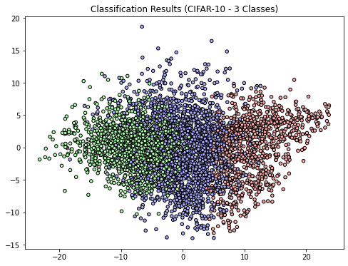
Figure 4. The classification of Cifar-10.

Example 4.5.

We tested our proposed method on 10 KEEL imbalanced benchmark data sets which contains different levels of imbalance in data and different sample sizes [1] as summarized in Table 3. In Table. 3 the column denoted by $n$ stands for the total number of samples, $p$ is the number of features, and IR indicates the ratio between majority and Minority class samples in each data set.

Table 3. Information of selected imbalanced benchmark datasets

Dataset	IR	$p$	$n$	%Minority
abalone9-18	16.40	8	731	5.74
appendicitis	4.04	7	106	19.81
ecoli2	5.46	7	336	15.47
hypo	15.49	6	2012	6.06
new-thyroid1	5.14	5	215	16.27
shuttle-c0-vs-c4	13.86	9	1829	6.72
sick	11.61	6	2751	7.92
vowel0	9.98	13	988	9.1
yeast3	8.10	8	1484	10.98

To evaluate our Algorithms, we use the metrics ${\rm F}_{1}$-Score, Recall, Accuracy and Precision for each classes. To ensure consistency for all experiments, for each benchmark, first, the data set is shuffled. Subsequently, 1 percent of the samples are randomly chosen in accordance with the dataset’s IR as the labeled samples. This process is independently repeated 100 times, then the averages of the previously mentioned metrics are computed. I should mention that for data set ”shuttle-c0-vs-c4” we choose 4 labels per class which is $0.43\%$ of data. We did not compare with existing schemas since most schemes with only $0.43\%$ of labeled samples per class give poor results.

Table 4 displays the comparison between performance of our proposed method, with Poisson Learning. For each data set, the second column indicates the number of samples randomly selected from each class as labeled data.

Table 4. Information of selected imbalanced benchmark datasets

Names	IGRF
Dataset	Accuracy	F1 min	F1 maj	Recall min	Recall maj	Precision min	Precision maj
yeast3	$.864$	$.524$	$.919$	$.693$	$.882$	$.421$	$.959$
appendicitis	$.758$	$.529$	$.837$	$.705$	$.771$	$.423$	$.917$
abalone9-18	$.9519$	$.7356$	$.9749$	$.7380$	$.9941$	$.7333$	$.9565$
ecoli2	$.875$	$.694$	$.922$	$.912$	$.869$	$.561$	$.982$
hypo	$.9024$	$.7257$	$.5657$	$.82352$	$.9169$	$.6488$	$.9407$
new-tyroid1	$.877$	$.425$	$.931$	$.278$	$.994$	$.898$	$.876$
shuttle-c0-vs-c4	.9737	.757	.986	.6097	.986	1	.970
sick	$.8146$	$.4044$	$.8196$	$.7833$	$.8196$	$.2725$	$.8197$
vowel0	$.725$	$.172$	$.835$	$.317$	$.766$	$.118$	$.919$

5. Conclusion

In this work, we present several schemes to enhance the efficacy of classification algorithms when dealing with large datasets with limited labeled data. The method leverage the efficiency of Poisson and Gaussian Random Fields methods while maintains simplicity and convergence.

The Modified Gaussian Random Fields (MGRF) and IGRF algorithms optimize label propagation across a graph by adjusting the initial label vector and iteratively refining the classification process. This approach demonstrates a substantial improvement.

The Improved Poisson Learning (IPL) algorithm, addresses the limitations of Poisson Learning by incorporating a subtraction of the matrix from the transition matrix, enhancing the stability and convergence of the label propagation process. This adjustment allows the algorithm to perform more effectively the case that data is imbalanced, ensuring that minority classes are represented and classified.