Learning System Dynamics without Forgetting

Abstract

Predicting the trajectories of systems with unknown dynamics (i.e. the governing rules) is crucial in various research fields, including physics and biology. This challenge has gathered significant attention from diverse communities. Most existing works focus on learning fixed system dynamics within one single system. However, real-world applications often involve multiple systems with different types of dynamics or evolving systems with non-stationary dynamics (dynamics shifts). When data from those systems are continuously collected and sequentially fed to machine learning models for training, these models tend to be biased toward the most recently learned dynamics, leading to catastrophic forgetting of previously observed/learned system dynamics. To this end, we aim to learn system dynamics via continual learning. Specifically, we present a novel framework of Mode-switching Graph ODE (MS-GODE), which can continually learn varying dynamics and encode the system-specific dynamics into binary masks over the model parameters. During the inference stage, the model can select the most confident mask based on the observational data to identify the system and predict future trajectories accordingly. Empirically, we systematically investigate the task configurations and compare the proposed MS-GODE with state-of-the-art techniques. More importantly, we construct a novel benchmark of biological dynamic systems, featuring diverse systems with disparate dynamics and significantly enriching the research field of machine learning for dynamic systems.

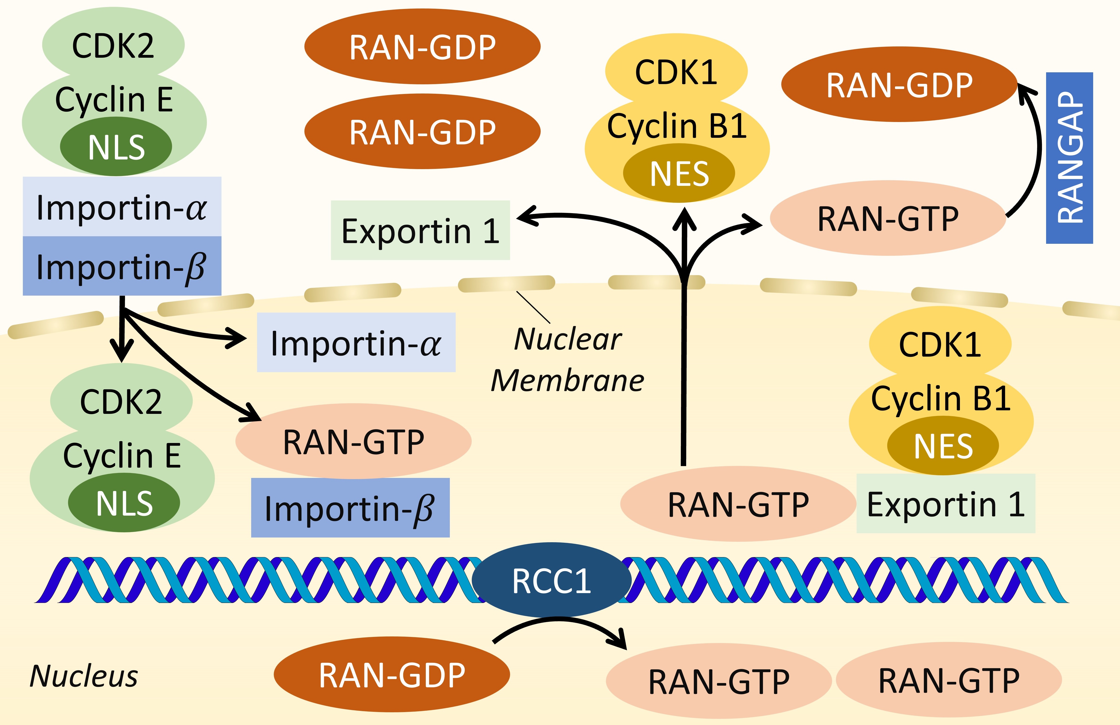
Figure 1: Illustration of one of the biological cellular systems involved in our work: RAN-regulated nucleocytoplasmic transport [1]. Briefly speaking, this model of translocation of a cargo protein via the nuclear pore is based on the Ran protein. In such systems, multiple factors could change and alter the entire dynamics.

1 Introduction

Scientific research often involves systems composed of interacting objects, such as multi-body systems in physics and cellular systems in biology, with their evolution governed by underlying dynamic rules. However, due to potentially unknown or incomplete dynamic rules or incomplete observations, deriving explicit equations to simulate system evolution can be extremely challenging. As a result, data-driven approaches based on machine learning have emerged as a promising solution for predicting the future trajectories of system states purely from observational data. For instance, the Interaction Network (IN) model [2] explicitly learns interactions between pairs of objects and has demonstrated superior performance in simulated physics systems, showcasing the potential of machine learning in studying physical system dynamics. IN has inspired many subsequent works [3, 4, 5, 6]. Later, to enable the modeling of incomplete and temporarily irregular system observations, ODE-based models [7, 8] were proposed to learn the continuous dynamics of the systems.

Despite the success of these methods, existing approaches typically assume the fixed type of dynamics within the target system. However, in many real-world scenarios, system dynamics are subject to change over time, or multiple systems may involve different types of dynamics. When data from those systems are continuously collected and sequentially fed to machine learning models for training, an ideal model is expected to continually learn varying dynamics without forgetting the previously observed ones and correctly infer any type of underlying dynamics during the test stage. For example, in cellular dynamics modeling (Figure 1), the dynamics of the same set of variables are subject to change when the kinetic factors change. Besides, a widely adopted task in dynamic system learning is predicting the trajectories of objects in an n-body system based on the observed trajectories [7, 2]. As illustrated in Figure 2, systems may be governed by different dynamics including various interaction types (e.g., elastic force or electrostatic force) and different interaction strengths (e.g., different amounts of charges on charged objects). In such scenarios, models that continually learn from systems with varying dynamics may encounter the catastrophic forgetting problem. In other words, the model can only accurately predict the most recently observed system dynamics while failing to predict earlier system dynamics due to forgetting.

Targeting the challenge, we propose a novel mode-switching graph ODE (MS-GODE) model, which can continually learn varying system dynamics and automatically switch to the corresponding mode during the test stage. Overall, MS-GODE follows the Variational AutoEncoder (VAE) [9] structure. Given the observational data, an encoder network first encodes the data into latent states, upon which an ODE-based generator predicts the future system trajectories within the latent space. Finally, a decoder network maps the predicted latent states back into the data space. This framework can effectively learn the continuous system dynamics and is suitable for system observations with irregular temporal sampling intervals, such as the biological systems studied in our work. However, for continual learning over different types of system dynamics, this framework alone is prone to catastrophic forgetting, as the new dynamic patterns may overwrite old knowledge encoded in the model parameters. Inspired by the advancements of sub-networks [10, 11, 12], we fix the model weights and optimize a unique binary mask over the parameters for each system during training. Unlike standard model training, which encodes learned patterns solely in model weights, each type of dynamics in MS-GODE is encoded in the topology of a sub-network (the binary mask), and the backbone with fixed weight values. In the test stage, the most suitable mask, which can most accurately reconstruct the given observation, is chosen and applied to the backbone network to form a system specific sub-network. This approach avoids catastrophic forgetting because the backbone network parameters are fixed, and system-specific knowledge is encoded in separate binary masks.

Besides the technical contribution, we have also created a novel dynamic system benchmark consisting of biological cellular systems based on the VCell platform [13, 14, 15]. Compared to the widely adopted simulated physics systems, cellular systems contain heterogeneous objects and interactions, offering richer and more challenging patterns of system dynamics. Therefore, the novel benchmark will significantly enhance the research of machine learning-based system dynamics prediction.

In experiments, we thoroughly investigate how the system sequence configuration influences the model performance when learning sequentially and then empirically demonstrate that our proposed MS-GODE outperforms existing state-of-the-art techniques.

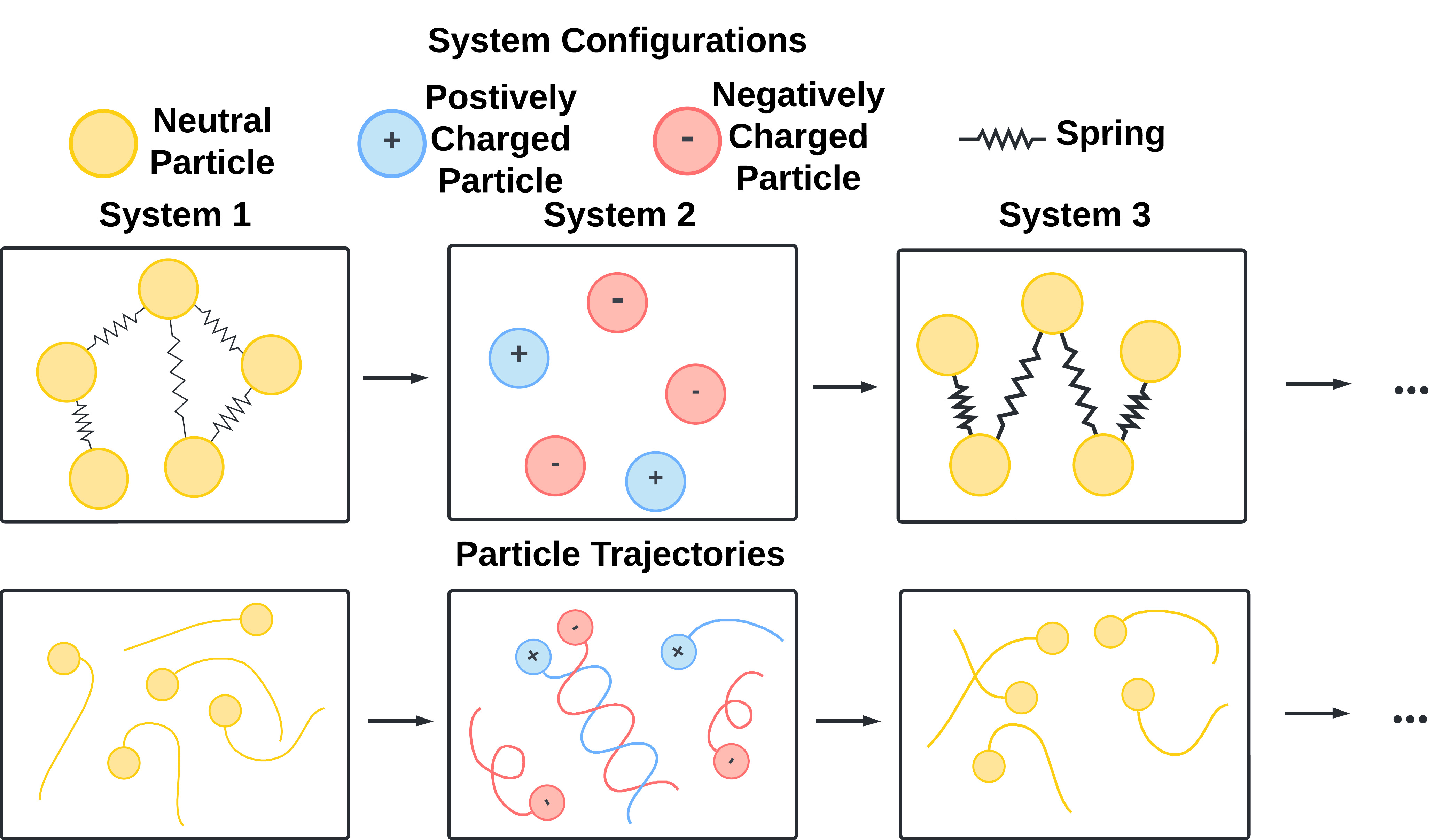
Figure 2: Illustration of the continual learning over different physics systems with different dynamics. The factors determining the dynamics shown in this figure include the type and strength of the interactions.

2 Related Works

2.1 Learning based dynamic System Prediction

In recent years, neural networks, especially graph neural networks (GNNs), have been proved to be promising in predicting the complex evolution of systems consisting of interacting objects [2, 3, 4, 5, 6]. This was firstly demonstrated by [2] with Interaction Network (IN), which iteratively infers the effects of the pair-wise interactions within a system and predicts the changes of the system states. Following IN, [3] proposed neural relational inference (NRI) to predict systems consisting of objects with unknown relationship. [16] proposed Hierarchical Relation Network (HRN) that extends the predictions to systems consisting of deformable objects. [4] proposed Hamiltonian ODE graph network (HOGN), which injects Hamiltonian mechanics into the model as a physically informed inductive bias. Later, to better consider the intrinsic symmetry of the target systems, GNNs with different invariance and equivariane are proposed [17, 5, 18, 19, 20, 6].

Considering that the observation of real-world systems may be incomplete and irregularly samples, [7] proposed LG-ODE, which is capable of generating continuous system dynamics based on the latent ordinary differential equations. Following LG-ODE, [8] proposed Coupled Graph ODE (CG-ODE) to further extend the continuous dynamics prediction to systems with unknown relationship. Similar ideas are also adopted in other time series research [21]. Our work is closely related to the ODE based models [21, 7, 8], and we also encode the system dynamics within the irregularly and partially observed data via spatial-temporal GNN structures [7, 8]. Although these above mentioned methods have made significant contributions to dynamic system prediction from different perspectives, they have been restricted to learning a single system with fixed dynamics.

2.2 Continual Learning & Masked Networks

Existing continual learning methods can be briefly categorized into three types [22, 23, 24, 25]. Regularization based methods slow down the adaption of important model parameters via regularization terms, so that the forgetting problem is alleviated [26, 27]. For example, Elastic Weight Consolidation (EWC) [28] and Memory Aware Synapses (MAS) [29] estimate the importance of the model parameters to the learned tasks, and add penalty terms to slow down the update rate of the parameters that are important to the previously learned tasks. Second, experience replay based methods replay the representative data stored from previous tasks to the model when learning new tasks to prevent forgetting [30, 31, 32, 33]. For example, Gradient Episodic Memory (GEM) [34] leverages the gradients computed based on the buffered data to modify the gradients for learning the current task and avoid the negative interference between learning different tasks. Finally, parameter isolation based methods gradually introduce new parameters to the model for new tasks to prevent the parameters that are important to previous tasks [35, 36]. For example, Progressive Neural Network (PNN) [37] allocate new network branches for new tasks, such that the learning on new tasks does not modify the parameters encoding knowledge of the old tasks. Our proposed MS-GODE also belongs to the parameter-isolation based methods, and is related to Supermasks in Superposition (SupSup) [12] and the edge-popup algorithm [11]. SupSup studies continual learning for classification tasks with an output entropy based mask selection, which is not applicable to our task. Edge-popup algorithm provides a simple yet efficient strategy to select a sub-network from the original network, and is adopted by us to optimize the binary masks over the model parameters. As far as we are concerned, existing continual learning works have not been applied to the dynamic system prediction targeted by this paper. Therefore, by customizing the representative continual learning techniques to our task as baselines, we also contribute to the community by extending the applicable areas of the existing methods and by demonstrating the advantages and disadvantages of different methods on a new task.

3 Learning System Dynamics without Forgetting

3.1 Preliminaries

In our work, the model is required to sequentially learn on multiple systems with different dynamics. Each system is composed of multiple interacting objects, therefore is naturally represented as a graph $\mathcal{G}=\{\mathbb{V},\mathbb{E}\}$. $\{\mathbb{V}$ is the node set denoting the objects of the systems, and $\mathbb{E}$ is the edge set containing the information of the relation and interaction between the objects. Based on the edge set $\mathbb{E}$, the spatial neighborhood of a node is defined as $\mathcal{N}_{s}(v)=\{u|e_{u,v}\in\mathbb{E}\}$. Each object node $v$ is accompanied with observational data containing the observed states at certain time steps $\mathbb{X}_{v}=\{\mathbf{x}_{v}^{t}|t\in\mathbb{T}_{v}\}$. With the system structured as a graph, the observation of the system evolution trajectory is naturally a spatial temporal graph, of which each node is an observed state $\mathbf{x}_{v}^{t}$. In the multi-body system example, the observation is the trajectories of the particles over time. In the following, we will refer to $\mathbf{x}_{v}^{t}$) as a ‘state’ for convenience. The set $\mathbb{T}_{v}$ contains the time steps (real numbers) when the states of $v$ are observed and can vary across different objects. For the prediction task, the observations lie within a certain period, i.e. $\bigcup_{v\in\mathbb{V}}\mathbb{T}_{v}\in$[$t_{0},t_{1}$], and the task is to predict the system states at future time steps beyond $t_{1}$. We denote the future time steps to predict for an object $v$ as $\mathbb{T}_{v}^{pred}$. In our continual dynamics learning setting, the training stage requires a model to sequentially learn on multiple systems with different dynamics and potentially different objects (i.e. $\mathbb{V}$).

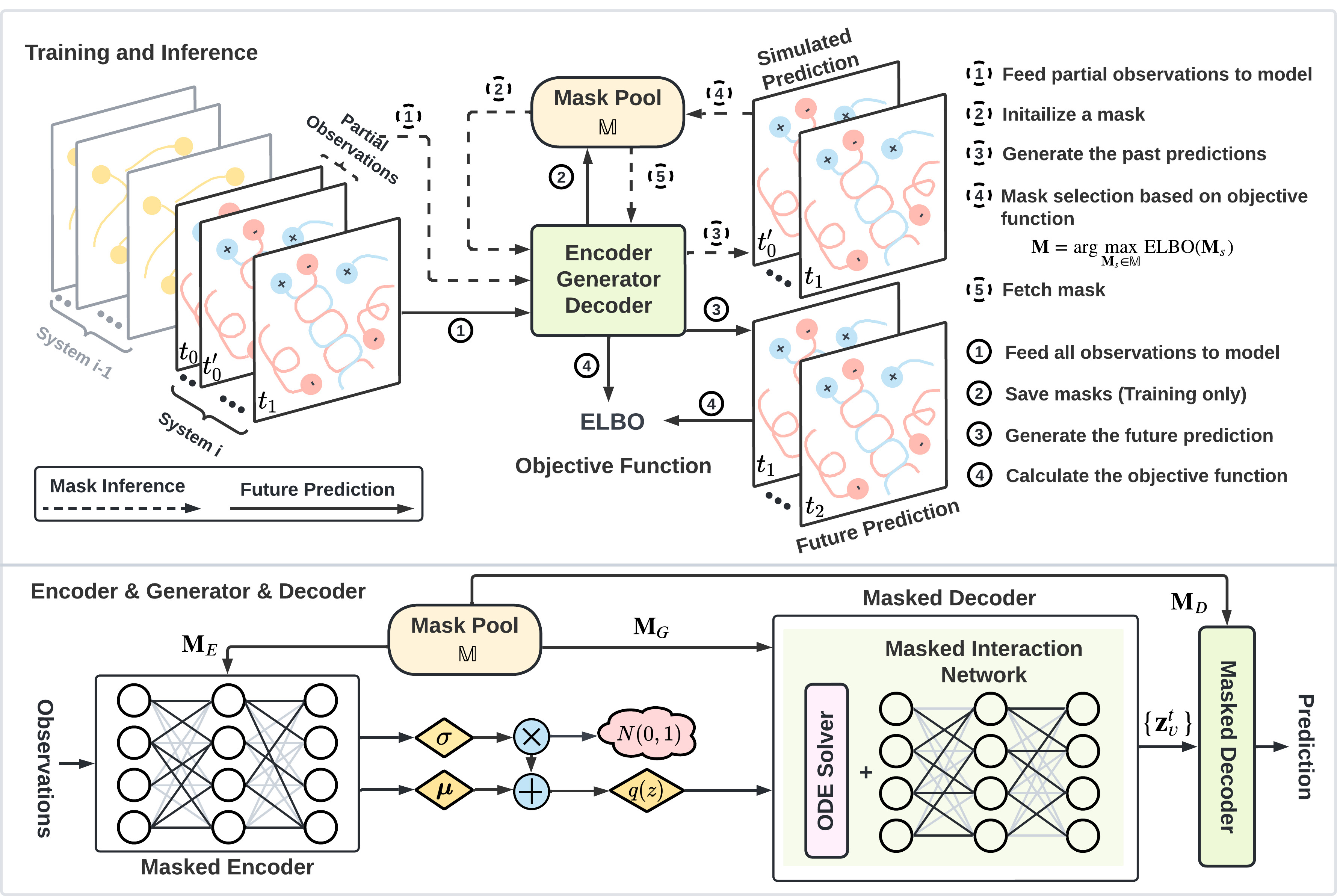
Figure 3: The upper part illustrates the workflow of MS-GODE during mask selection and inference, which are denoted by dashed and solid lines. During mask selection, the observation is split into two parts, and the first part is fed into the model for selecting the mask that can best predict the second part (simulated prediction). During inference, the entire observation is fed into the model to predict the unknown future states. The lower part demonstrates the structure of the masked encoder, masked generator, and masked decoder. Different components fetch their corresponding mask from the mask pool and apply the mask onto the parameters.

3.2 Framework Overview

In this subsection, we provide a high-level introduction on the workflow of MS-GODE (Figure 3), while the details of each component are provided in the following subsections.

Overall, MS-GODE consists of three core components: 1) An encoder network $\mathrm{Enc}(\cdot;\theta_{E})$ parameterized by the parameters $\theta_{E}$ for encoding the observational data into the latent space; 2) A ODE-based generator $\mathrm{Gen}(\cdot;\theta_{G})$ parameterized by $\theta_{G}$ for predicting the future states of the system within the latent space; 3) A decoder network $\mathrm{Dec}(\cdot;\theta_{D})$ parameterized by $\theta_{D}$ for transforming the predicted latent states back into the data space. Within a standard learning scheme, the model will be trained and optimized by updating the parameters $\{\theta_{E},\theta_{G},\theta_{D}\}$. However, as introduced above, when continually training the model on multiple systems with different dynamics, this learning scheme will bias the model towards the most recently observed system, causing the catastrophic forgetting problem. In this work, inspired by the recent advances in sub-network learning [11], we propose to avoid directly optimizing the parameters $\{\theta_{E},\theta_{G},\theta_{D}\}$. Instead, we train the model by optimizing the connection topology of the backbone model and encode the dynamics of each system into a sub-network. This is equivalent to encoding each system-specific dynamics pattern into a binary mask overlaying the shared parameters with fixed values. In this way, the interference between learning on different systems with different dynamics, i.e. the cause of the forgetting problem, can be avoided. Moreover, this approach is also memory efficient since the space for storing the binary masks is negligible. With the system-specific masks, the three model components are formulated as:

$$\mathrm{Enc}(\cdot;\theta_{E}\odot\mathbf{M}_{E}^{s});\quad\mathrm{Gen}(\cdot;\theta_{G}\odot\mathbf{M}_{G}^{s});\quad\mathrm{Dec}(\cdot;\theta_{D}\odot\mathbf{M}_{D}^{s}),$$ (1)

where the superscript $s$ is the system index. The details of the binary mask optimization during training and mask selection during testing are provided in Section 3.5. In the following subsections, all parameters are subsets of $\theta_{E}$, $\theta_{G}$, or $\theta_{D}$ and are controlled by the corresponding masks. For example, $\mathbf{W}_{msg}$ in Section 3.3 is part of the encoder parameters $\theta_{E}$ and is under the control of $\mathbf{M}_{E}^{s}$.

3.3 Masked Encoder Network

As the first component of the model, the masked encoder network serves to encode the dynamic pattern in the observational data into the latent space. As introduced in Section 3.1, the observation of the system is a spatial temporal graph. Therefore, we adopt the attention-based spatial temporal graph neural network framework (ST-GNN) [38, 7, 8, 39] to encode the observational data. Originally, the graph attention network (GAT) [40] is designed to aggregate information over the spatially neighboring nodes. On spatial temporal graphs, the information aggregation is extended to both spatial and temporal neighboring nodes. Such a spatial temporal neighborhood of a state $\mathbf{x}_{v}^{t}$ is defined as the states of the spatially connected nodes within a specified temporal window $\delta_{window}$,

$$\mathcal{N}_{st}(\mathbf{x}_{v}^{t}):=\{\mathbf{x}_{w}^{q}|e_{u,v}\in\mathbb{E}\quad and\quad|q-t|<\delta_{window}\}.$$ (2)

Then, the information aggregation is conducted over the spatial temporal neighborhood to iteratively update the representation of each state. Formally, the update of the hidden representation of a state $\mathbf{x}_{v}^{t}$ at the $l$-the layer of the ST-GNN is formulated as,

$$\mathbf{h}_{v,t}^{l}=\mathbf{h}_{v,t}^{l-1}+\sigma(\sum_{x_{u}^{q}\in\mathcal{N}_{st}(\mathbf{x}_{v}^{t})}\mathrm{a}(\mathbf{h}_{v,t}^{l-1},\mathbf{h}_{u,q}^{l-1},q-t)\cdot\mathbf{W}_{msg}\cdot\mathrm{msg}(\mathbf{h}_{u,t}^{l-1},q-t)),$$ (3)

where $\mathrm{a}(\cdot,\cdot)$ calculates the attention score between a pair of states, and $\mathrm{msg}(\cdot,\cdot)$ is the message function commonly adopted in graph neural networks [41]. However, different from the message function in typical graph neural networks, the temporal relationship between the states is a crucial part to understand the system dynamics in our task. Therefore, we follow the strategy in LG-ODE [7] to incorporate the temporal distance between the states in the message function and attention function,

$$\mathrm{msg}(\mathbf{h}_{u,t}^{l-1},q-t)):=\sigma(\mathbf{W}_{tmp}\cdot\mathrm{concat}(\mathbf{h}_{u,t}^{l-1},q-t))+\mathrm{TE}(q-t),$$ (4)

$$\mathrm{a}(\mathbf{h}_{v,t}^{l-1},\mathbf{h}_{u,q}^{l-1},q-t):=\frac{\exp(\mathrm{msg}(\mathbf{h}_{u,q}^{l-1},q-t))^{T}\cdot\mathbf{h}_{v,t}^{l-1})}{\sum_{x_{w}^{p}\in\mathcal{N}_{st}(\mathbf{x}_{v}^{t})}\exp(\mathrm{msg}(\mathbf{h}_{w,p}^{l-1},p-t))^{T}\cdot\mathbf{h}_{v,t}^{l-1})},$$ (5)

where $\mathrm{TE(\cdot)}$ is a temporal position encoding developed based on the position encoding in Transformer [42] for incorporating the temporal information into the representation. Finally, for the subsequent state prediction task, the representations of the states are averaged over the temporal dimension,

$$\mathbf{h}_{final}^{v}=\frac{1}{|\mathbb{T}_{v}|}\sum_{t\in\mathbb{T}_{v}}\sigma(\bar{\mathbf{h}}_{v}^{T}\cdot\mathrm{msg}(\mathbf{h}_{v,t}^{L}))\cdot\mathrm{msg}(\mathbf{h}_{v,t}^{L},t-t_{0}),$$ (6)

where $t_{0}$ denotes the starting time of all states in the observational data (Section 3.1), and the average term $\bar{\mathbf{h}}_{v}$ of each node $v$ is calculated by weighted summation over the representations at all time steps,

$$\bar{\mathbf{h}}_{v}=\sigma(\frac{1}{|\mathbb{T}_{v}|}\sum_{t\in\mathbb{T}_{v}}\mathrm{msg}(\mathbf{h}_{v,t}^{L},t-t_{0})\cdot\mathbf{W}_{avg}).$$ (7)

3.4 Masked ODE-based Generator

For practical consideration, we develop the masked ODE-based generator based on the latent ODE framework [43, 7, 21], such that the model can handle observation with irregular temporal intervals and predict future states at any time denoted by real numbers. Specifically, the trajectory prediction problem is formulated as as solving an ODE initial value problem (IVP), where the initial values of the objects ($\{z_{v}^{t_{1}}|v\in\mathbb{V}\}$) are generated from the final representation of the observational data ($\{\mathbf{h}_{final}^{v}|v\in\mathbb{V}\}$, Section 3.3). Mathematically, the procedure of predicting the future trajectory of a system $s$ is formulated as,

$$\quad\quad\quad\quad\quad\quad\quad\quad\quad\quad z_{v}^{t_{1}}\sim\mathrm{p}(z_{v}^{t_{1}}),v\in\mathbb{V}$$ (8)

$$\{z_{v}^{\tau}|v\in\mathbb{V},\tau\in\mathbb{T}_{v}^{pred}\}=\mathrm{Gen}(\{z_{v}^{t_{1}}|v\in\mathbb{V}\},\{\mathbb{T}_{v}^{pred}|v\in\mathbb{V}\};\theta_{G}\odot\mathbf{M}_{G}^{s})),$$ (9)

To estimate the posterior distribution $q(\{z_{v}^{t_{1}}|v\in\mathbb{V}\}|\{\mathbb{X}_{v}|v\in\mathbb{V}\})$ based on the observation (i.e. $\{\mathbb{X}_{v}|v\in\mathbb{V}\}$), the distribution is assumed to be Gaussian. Then the mean $\mu_{v}$ and standard deviation $\sigma_{v}$ are generated from $\{\mathbf{h}_{final}^{v}|v\in\mathbb{V}\}$ with a multi-layer perceptron (MLP),

$$q(z_{v}^{t_{1}}|\{\mathbb{X}_{v}|v\in\mathbb{V}\})=\mathcal{N}(\mu_{v},\sigma_{v})=\mathcal{N}(\mathrm{mlp}(\mathbf{h}_{final}^{v};\theta_{G}\odot\mathbf{M}_{G}^{s})),v\in\mathbb{V}.$$ (10)

As noted at the end of Section 3.2, the parameters of $\mathrm{mlp}(\cdot)$ and $\mathrm{F}_{int}(\cdot)$ are part of $\theta_{G}$ and controlled by $\mathbf{M}_{G}^{s}$.

Based on the approximate posterior distribution $q(\{z_{v}^{t_{1}}|v\in\mathbb{V}\}|\{\mathbb{X}_{v}|v\in\mathbb{V}\})$, we sample an initial state for each object, upon which the ODE solver will be applied for generating the predicted states in the latent space. The dynamics of each object in the system is governed by its interaction with all the other objects. Therefore, the core part of the ODE-based generator is a trainable interaction network that encodes the dynamics in the form of the derivative of each $\mathbf{z}_{v}$,

$$\frac{\mathrm{d}\mathbf{z}_{v}}{\mathrm{d}t}|_{t=t^{\prime}}=\mathrm{F}_{int}(\{\mathbf{z}_{u}^{t^{\prime}}|u\in\mathcal{N}_{s}(v)\};\theta_{G}\odot\mathbf{M}_{G}),$$ (11)

where the function $\mathrm{F}_{int}(\cdot)$ parameterized by $\theta_{I}$ predicts the dynamics (derivative) of each object $v$ based on all the other objects interacting with $v$ (i.e. $\mathcal{N}_{s}(v)$ defined in Section 3.1), and $t^{\prime}$ denotes any possible future time. Note that $\mathcal{N}_{s}(v)$ only contains the spatial neighbors and is different from $\mathcal{N}_{st}(\cdot)$. Because the object-wise interaction at a certain time $t^{\prime}$ is not dependent on system states at other times. For example, in a charged particle system governed by electrostatic force, the force between each pair of particle at $t^{\prime}$ is solely determined by the relative positions (i.e. the states) of the particles (Figure 2) at $t^{\prime}$. In our work, we adopt the Neural Relational Inference (NRI) [3] as the function $\mathrm{F}_{int}(\cdot)$. Based on $\mathrm{F}_{int}(\cdot)$, the future state of the system at an arbitrary future time $t_{2}$ can be obtained via an integration

$$\mathbf{z}_{v}^{t_{2}}=\mathbf{z}_{v}^{t_{1}}+\int_{t_{1}}^{t_{2}}\frac{\mathrm{d}\mathbf{z}_{v}}{\mathrm{d}t}\mathrm{d}t=\mathbf{z}_{v}^{t_{1}}+\int_{t_{1}}^{t_{2}}\mathrm{F}_{int}(\{\mathbf{z}_{u}^{t}|u\in\mathcal{N}_{s}(v)\};\theta_{G}\odot\mathbf{M}_{G})\mathrm{d}t,$$ (12)

which can be solved numerically by mature ODE solvers, e.g. Runge-Kutta method. After obtaining the latent representations of the states at the future time steps ($\{\mathbf{z}_{v}^{t}|t\in\mathbb{T}_{future},v\in\mathbb{V}\}$), the predictions are generated via a masked decoder network that projects the latent representations back into the data space

$$\mathbf{y}_{v}^{t}=\mathrm{Dec}(\mathbf{z}_{v}^{t};\theta_{D}\odot\mathbf{M}_{D}),t\in\mathbb{T}_{future},v\in\mathbb{V}.$$ (13)

In our work, $\mathrm{Dec}(\cdot;\theta_{D})$ is instantiated as a multi-layer perceptron (MLP).

3.5 Mask Optimization & Selection

MS-GODE is trained by maximizing the Evidence Lower Bound (ELBO). Denoting the concatenation of all the initial latent states ($\{\mathbf{z}_{v}^{t_{1}}|v\in\mathbb{V}\}$) as $\mathbf{Z}_{\mathbb{V}}^{t_{1}}$, the ELBO is formulated as

$$\mathrm{ELBO}(\mathbf{M}^{s}) =\mathbb{E}_{\mathbf{Z}_{\mathbb{V}}^{t_{1}}\sim q(z_{v}^{t_{1}}|\{\mathbb{X}_{v}|v\in\mathbb{V}\})}[\log(p(\{\mathbf{x}_{v}^{t}|t\in\mathbb{T}_{future},v\in\mathbb{V}\}))]$$ (14)

$$-\mathbf{KL}[q(\mathbf{Z}_{\mathbb{V}}^{t_{1}}|\{\mathbb{X}_{v}|v\in\mathbb{V}\}))||p(\mathbf{Z}_{\mathbb{V}}^{t_{1}})].$$ (15)

where $p(\mathbf{Z}_{\mathbb{V}}^{t_{1}})$ denotes the prior distribution of $\mathbf{Z}_{\mathbb{V}}^{t_{1}}$, which is typically chosen as standard Gaussian. $\mathbf{M}^{s}$ denotes the union of all masks over different modules of the framework (i.e. $\mathbf{M}^{s}=\{\mathbf{M}_{E}^{s},\mathbf{M}_{I}^{s},\mathbf{M}_{P}^{s}\}$). In our model, the parameters ($\theta_{E}$,$\theta_{I}$, and $\theta_{P}$) will be fixed, and the ELBO will be maximized by optimizing the binary masks $\mathbf{M}^{s}$ overlaying the parameters via the Edge-popup algorithm [11]. After learning each system, the obtained mask is added into a mask pool $\mathbb{M}$ to be used in testing. During testing, MS-GODE will automatically select the most appropriate mask based on the confidence of reconstructing part of the given observations. Specifically, a given observations from [$t_{0}$,$t_{1}$] is first split it into two periods [$t_{0}$,$\frac{t_{0}+t_{1}}{2}$] and [$\frac{t_{0}+t_{1}}{2}$,$t_{1}$]. Then, the first half is fed into the model and the correct mask can be chosen by selecting the one that can reconstruct the second half with the lowest error.

4 Experiments

In this section, we aim to answer the following questions. 1. How to properly configure MS-GODE for optimal performance. 2. How would the configuration of the system sequence influence the performance? 3. How is the performance of the existing CL techniques? 4. Can MS-GODE outperform the baselines?

4.1 Experimental Systems

In experiments, we adopt physics and biological cellular systems. The detailed introduction on the system sequence construction is provided in Appendix A.1.

Simulated physics systems are commonly adopted to evaluate the machine learning models in the task of learning system dynamics [6, 2, 7]. The physics systems adopted in this work include spring connected particles and charged particles (Figure 2). We carefully adjust the system configuration and construct 3 system sequences with different level of dynamics shift (Appendix A.1).

Biological cellular systems are innovatively introduced in this work based on Virtual Cell platform [13, 14, 15]. In experiments, we adopt two models: EGFR receptor interaction model and Ran protein based translocation model. We adjust the coefficients of the models to construct a sequence containing 2 EGFR and 2 Ran systems interleaved with each other ($\mathrm{EGFR}_{1}\rightarrow\mathrm{Ran}_{1}\rightarrow\mathrm{EGFR}_{2}\rightarrow\mathrm{Ran}_{2}$). Full details are provided in Appendix A.1.2.

4.2 Experimental Setups & Evaluation

Model evaluation under the continual learning setting. Different from standard learning setting, the models in this paper learns sequentially on multiple systems under the continual learning and evaluation are significantly different. After learning each new task, the model is tested on all learned tasks and the results form a performance matrix $\mathrm{M}^{p}\in\mathbb{R}^{N\times N}$, where $\mathrm{M}^{p}_{i,j}$ denotes the performance on the $j$-system after learning from the $1$-st to the $i$-th system, and $N$ is the number of systems in the sequence. In our experiments, each entry of $\mathrm{M}^{p}$ is a mean square error (MSE) evaluating the performance on a single system. To evaluate the performance over all systems, average performance (AM) can be calculated. For example, $\frac{\sum_{j=1}^{i}\mathrm{M}^{p}_{N,j}}{N}$ is the average performance after learning the entire sequence with $N$ tasks. Similarly, average forgetting (AF) can be calculated as $\frac{\sum_{j=1}^{N-1}\mathrm{M}^{p}_{N,j}-\mathrm{M}^{p}_{j,j}}{N-1}$. More details on model evaluation can be found in Appendix A.4. All experiments are repeated 5 times on a Nvidia Titan Xp GPU. The results are reported with average and standard deviations.

Baselines & model settings. We adopt state-of-the-arts baselines including the performance upper (joint training) and lower bounds (fine-tune) in experiments. The state-of-the-arts baselines adopted in this work include Elastic Weight Consolidation (EWC) [28] based on regularization, Learning without Forgetting (LwF) [44] based on knowledge distillation, Gradient Episodic Memory (GEM) [34] based on both memory replay and regularization, Bias-Correction [45] based Memory Replay (BCMR) that integrates the idea of data sampling bias correction into memory replay, and Scheduled Data Prior (SDP) [46] that adopts a data-driven approach to balance the contribution of past and current data. Besides, joint training and fine-tune are commonly adopted in continual learning works. Joint training trains the model jointly over all systems, which does not follow the continual learning setting. Fine-tune directly trains the model incrementally on new systems without any continual learning technique.

More details of experimental settings and baselines and experimental settings are provided in Appendix A.1 A.3.

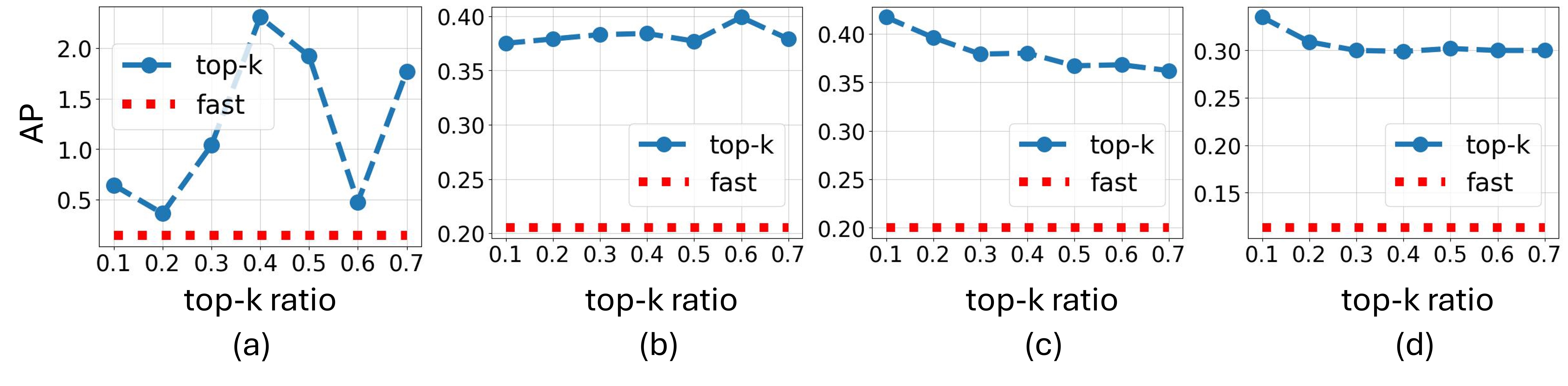
Figure 4: Performance comparison among different strategies to binarize the mask values. (a) Comparison over the cellular system sequence $\mathrm{EGFR}_{1}\rightarrow\mathrm{Ran}_{1}\rightarrow\mathrm{EGFR}_{2}\rightarrow\mathrm{Ran}_{2}$. (b)(c)(d) Comparison over different physics system sequences. Blue line denotes the performance of top-k selection with different thresholds. Red line demonstrates the performance of using fast selection.

Figure 5: AP (a) and AF (b) of MS-GODE with different dropout rate.

4.3 Model Configuration and Performance (RQ1)

When optimizing the system-specific masks using the edge-popup algorithm [11] (Appendix A.2), each entry of the mask is assigned with a continuous value for gradient descent after backpropagation. During inference, different strategies can be adopted to transform the continuous scores into binary values. In our experiments, we tested both ‘fast selection’ and ‘top-k selection’ with different thresholds. ‘Fast selection’ set all entries with positive score values into ‘1’s and the other entries into ‘0’s. ‘Top-k selection’ first ranks the score values and set a specified ratio of entries with the largest values into ‘1’s. In Figure 4, we show the performance of different strategies. Overall, ‘top-k selection’ is inferior to ‘fast selection’. This is potentially because that ‘fast selection’ does not limit the number of selected entries, therefore allowing more flexibility for optimization. We also observe that the performance of ‘top-k’ selection is more sensitive on the cellular systems compared to the physics systems, indicating that the cellular systems have higher optimization difficulty for sub-network (binary mask) learning over system sequences.

Second, sub-network learning will deactivate some neurons in the model, which resembles the dropout mechanism widely adopted in machine learning models and may cause the model to be over sparsified. Therefore, we investigate the influence of dropout rate in MS-GODE. From Figure 5, we could see that smaller dropout rate results in lower error (better performance). This corroborates our hypothesis that the mask selection mechanism and dropout are complementing each other, and the dropout rate should be decreased when the masking strategy is adopted.

Table 1: Performance comparisons on physics system sequences ($\downarrow$ lower means better).

Method	Seq1: Low-level dynamics shift		Seq2: Mid-level dynamics shift		Seq3: High-level dynamics shift
	AP $\downarrow$	AF $\downarrow$	AP $\downarrow$	AF /% $\downarrow$	AP $\downarrow$	AF /% $\downarrow$
Fine-tune	0.369$\pm$0.027	0.115$\pm$0.016	0.391$\pm$0.044	0.314$\pm$0.030	0.258$\pm$0.025	0.086$\pm$0.037
EWC [28]	0.208$\pm$0.015	-0.007$\pm$0.019	0.227$\pm$0.038	0.008$\pm$0.022	0.148$\pm$0.011	0.008$\pm$0.017
GEM [34]	0.251$\pm$0.037	0.079$\pm$0.020	0.379$\pm$0.023	0.302$\pm$0.030	0.163$\pm$0.037	-0.091$\pm$0.033
LwF [44]	0.258$\pm$0.011	0.104$\pm$0.042	0.363$\pm$0.039	0.312$\pm$0.042	0.130$\pm$0.025	0.016$\pm$0.032
BCMR [45]	0.284$\pm$0.017	-0.006$\pm$0.031	0.298$\pm$0.028	-0.001$\pm$0.033	0.233$\pm$0.017	0.027$\pm$0.023
SDP [46]	0.352$\pm$0.021	0.121$\pm$0.018	0.303$\pm$0.026	0.352$\pm$0.058	0.213$\pm$0.035	0.024$\pm$0.045
Joint	0.194$\pm$0.006	-	0.186$\pm$0.015	-	0.116$\pm$0.009	-
Ours	0.200$\pm$0.003	0.002$\pm$0.004	0.204$\pm$0.005	-0.001$\pm$0.001	0.113$\pm$0.001	-0.000$\pm$0.000

Table 2: Performance comparisons on biological cellular systems ($\downarrow$ lower means better).

Method	$\mathrm{EGFR}_{1}\rightarrow\mathrm{Ran}_{1}\rightarrow\mathrm{EGFR}_{2}\rightarrow\mathrm{Ran}_{2}$
	AP $\downarrow$	AF $\downarrow$
Fine-tune	0.355$\pm$0.089	0.226$\pm$0.037
EWC [28]	0.312$\pm$0.028	-0.013$\pm$0.019
GEM [34]	0.316$\pm$0.083	0.352$\pm$0.109
LwF [44]	0.330$\pm$0.036	0.349$\pm$0.046
BCMR [45]	0.149$\pm$0.025	0.013$\pm$0.044
SDP [46]	0.197$\pm$0.025	0.167$\pm$0.045
Joint	0.055$\pm$<0.001	-
Ours	0.144$\pm$0.012	-0.003$\pm$0.036

4.4 Sequence Configuration and Performance (RQ2)

In this subsection, we investigate the influence of system sequence configuration on the learning difficulty and model performance. Specifically, we construct 3 physics system sequences with increasing level of dynamics shift (Details are provided in Appendix A.1.1). Sequence 1 (low-level dynamics shift) consists of 8 spring connected particle systems, in which consecutive systems are only different in one system coefficient. Sequence 2 (mid-level dynamics shift) is constructed to have higher level of dynamics shift by simultaneously varying 2 system coefficients. Finally, sequence 3 (high-level dynamics shift) is constructed by interleaving spring connected particle systems and charged particle systems with disparate dynamics. As shown in Table 1, in terms of both AP and AF, most methods, including MS-GODE, obtain similar performance over Sequence 1 and 2, and obtain better performance on sequence 3. This is reasonable for MS-GODE, since the systems with more diverse dynamics are easier to distinguish for selecting the masks during inference. For the other baselines, e.g. Fine-tune, the results indicate that diverse systems may guide the model to exploit different parameters for different systems, while similar systems may cause the same part of parameters to be updated more frequently, resulting in more severe forgetting issue.

4.5 Comparisons with State-of-the-Arts (RQ3,4)

In this subsection, we compare MS-GODE with multiple state-of-the-arts methods including the joint training, which is typically regarded as the upper bound on the performance in continual learning research. The experiments are conducted on both physics systems 1 and cellular systems 2, which demonstrate that MS-GODE outperforms the baselines in both cellular systems and physics systems with different configurations. Besides, by comparing the results across different sequences in the two tables, we could find that the sequences with gradual dynamics shift (Sequence 1,2 of physics systems) are more difficult to learn than the sequences with abrupt dynamics shift (Sequence 3 of the physics systems and the cellular system).

4.6 In-depth Investigation on the Learning Dynamics (RQ3,4)

Table 1 and 2 provide the overall performance, which is convenient to compare different methods. However, as introduced in Section 4.2, to obtain an in-depth understanding of the performance of different methods, we have to seek help from the most through metric, i.e. the performance matrix. In Figure 6, we visualize the performance marices of different methods after learning different system sequences. The $i$-th column demonstrates the performance of the $i$-th task when learning sequentially over the systems. Comparing MS-GODE ((a) and (e)) and the other methods, we find that MS-GODE could maintain a much more stable performance of each system when learning over the sequence. EWC ((c) and (f)) also maintains a relatively stable performance of each system based on its regularization strategy. However, compared to MS-GODE, the model becomes less and less adaptive to new systems (the columns become increasingly darker from left to right). This is because the regularization is applied to more parameters when proceeding to each new task. Fine-tune ((b) and (g)) is not limited by regularization, therefore is more adaptive on new systems but less capable in preserving the performance on previous systems compared to EWC. LwF (d), although based on knowledge distillation, does not directly limit the adaptation of the parameters like EWC. Finally, based on memory and gradient modification, GEM (h) maintains the performance better than fine-tune (g), and is more adaptive to new tasks than EWC (f). More details on the performance matrices is provided in Appendix A.5.

Figure 6: Visualization of performance matrices. (a), (b), (c), (d) are performance of MS-GODE, fine-tune, EWC, and LwF on the cellular system sequence. (e), (f), (g), (h) are the performance of MS-GODE, EWC, fine-tune, and GEM, on the physics systems.

5 Conclusion

In this paper, we systematically study the problem of continually learning varying system dynamics, and propose an effective method MS-GODE for this task. Moreover, we also construct a novel benchmark consisting of biological cellular systems for the field of machine learning on system dynamics. Finally, we conduct comprehensive experiments on both physics and cellular system sequences, which not only demonstrate the effectiveness of MS-GODE, but also provide insights into the problem of machine learning over system sequences with dynamics shift. Although MS-GODE outperforms the baselines significantly, there is still a gap between MS-GODE and the performance upper bound (joint training) especially in the biological cellular systems. In our future work, we aim to develop improved strategies for sub-network learning to further boost the performance in both individual systems and system sequences.

Appendix A Appendix / supplemental material

A.1 System Sequence Configuration

A.1.1 Physics System Sequence

Simulated physics systems are commonly adopted to evaluate the machine learning models in the task of learning system dynamics [6, 2, 7]. The physics systems adopted in this work include spring connected particles and charged particles (Figure 2) with disparate dynamics, therefore are ideal for constructing system sequences to evaluate a model’s continual learning capability under severe significant dynamics shift. Besides, the configuration of each system type is also adjustable. For the spring connected particles, the number of particles, strength of the springs, and the size of the box containing the particles are adjustable. For the charged particles, the number of particles, charge sign, and the size of box are adjustable. In our experiments, we constructed multiple systems with different configurations, which are aligned into sequences for the model to learn.

The physics system sequences are constructed to have different types of dynamics changes. System sequence 1 is composed of 8 spring connected particle systems. Each system contains 5 particles, and some pairs of particles are connected by springs. An illustration is given in Figure 2. For each system, besides the number of particles, the size of the box containing the particles and the strength of spring are adjustable. In Sequence 1, the first 4 systems have constant spring strength and decreasing box size. From the $5$-th system, the box size is fixed, and the spring strength is gradually increased. Sequence 2 also contains 8 systems of spring connected particles and is designed to posses more severe dynamics shift. Specifically, both the box size and spring strength vary from the first to the last system, and the values are randomly aligned instead of monotonically increasing or decreasing. Sequence 3 is designed to posses more significant dynamics shift than Sequence 2 by incorporating the charged particle systems in the sequence. Specifically, Sequence 3 contains 4 spring connected particle systems and 4 charged particle systems, which are aligned alternatively. The box size gradually decreases and the interaction strength (spring strength or amount of charge on the particles) gradually increases. In a charged particle system, the particles could carry either positive or negative charge, and the system dynamics is governed by electrostatic force, which is significantly different from the spring connected particle system.

Specifically, we list the configurations of the systems in Table 3 and 4. Then the three sequences can be precisely represented as:

1. Sequence 1: $S_{1}\rightarrow S_{2}\rightarrow S_{3}\rightarrow S_{4}\rightarrow S_{5}\rightarrow S_{6}\rightarrow S_{7}\rightarrow S_{8}$

2. Sequence 2: $S_{1}\rightarrow S_{8}\rightarrow S_{2}\rightarrow S_{7}\rightarrow S_{3}\rightarrow S_{6}\rightarrow S_{5}\rightarrow S_{5}$

3. Sequence 3: $S_{1}\rightarrow C_{1}\rightarrow S_{9}\rightarrow C_{2}\rightarrow S_{10}\rightarrow C_{3}\rightarrow S_{8}\rightarrow C_{4}$

For each system, the simulation runs for 6,000 steps, and the observation is sampled every 100 steps, resulting in a 60-step series. During training, the first 60% part of the trajectory of each system is fed to the model to generate prediction for the remaining 40%. For each system sequence, 1,000 sequences are used for training, and another 1,000 sequences are used for testing.

System	S1	S2	S3	S4	S5	S6	S7	S8	S9	S10
Type	Spring	Spring	Spring	Spring	Spring	Spring	Spring	Spring	Spring	Spring
# particles	5	5	5	5	5	5	5	5	5	5
Box size	10.0	5.0	3.0	1.0	0.5	0.5	0.5	0.5	3.0	1.0
Interaction strength	0.01	0.01	0.01	0.01	0.01	0.1	0.5	1.0	0.1	0.5

Table 3: Spring connected system configurations.

System	C1	C2	C3	C4
Type	Charge	Charge	Charge	Charge
# particles	5	5	5	5
Box size	10.0	3.0	1.0	0.5
Interaction strength	0.01	0.1	0.5	1.0

Table 4: Charged particle system configurations.

A.1.2 Biological Cellular System

In this paper, we build a novel benchmark containing biological cellular dynamic systems based on Virtual Cell [13, 14, 15] with different system configurations and variable selection. Currently, the benchmark is built based on two types of cellular models. The first one is rule-based model of EGFR receptor interaction with two adapter proteins Grb2 and Shc. The second is a compartmental rule based model of translocation through the nuclear pore of a cargo protein based on the Ran protein (GTPase). Detailed description of these two systems can be found via https://vcell.org/webstart/VCell_Tutorials/VCell6.1_Rule-Based_Tutorial.pdf and https://vcell.org/webstart/VCell_Tutorials/VCell6.1_Rule-Based_Ran_Transport_Tutorial.pdf. Based on these 2 types of models, we construct multiple systems, which are aligned into different system sequences.

In our experiments, we adjust the parameter configurations of these two types of models to construct multiple systems with different dynamics, which are aligned into a sequence for the experiments. We generate simulated data using the Virtual Cell platform (VCell) and pre-process the data. In experiments, we adopt a 4-system sequence using the simulated data by alternatively align 2 EGFR systems and 2 Ran systems. EGFR system is rule-based model of EGFR receptor interaction with two adapter proteins Grb2 and Shc. Ran system is a compartmental rule based model of translocation through the nuclear pore of a cargo protein based on the Ran protein (GTPase).

For each cellular system, we generate 100 iterations of simulation using VCell. Different from the physics systems, the temporal interval between two time steps of cellular system is not constant. Similar to the physics systems, the first 60% part of the observation of each system simulation is fed into the model to reconstruct the remaining 40% during training. For each system, we generate 20 systems for training and 20 systems for testing.

A.1.3 Additional Details of Experimental Settings

For the encoder network, the number of layers is 2, and the hidden dimension is 64. 1 head is used for the attention mechanism. The interaction network of the generator is configured as 1-layer network, and the number of hidden dimensions is 128. Finally, the decoder network is a fully-connected layer. The model is trained for 20 epochs over each system in the given sequence. We adopt the AdamW optimizer [47] and set the learning rate as 0.0005.

A.2 Edge-popup Algorithm

In this work, we adopt the edge-popup algorithm [11] for optimizing the binary masks. The main idea is to optimize a continuous score value for each entry of the mask during the backpropagation, and binarize the values into discrete binary values during forward propagation (Appendix A.2). Accordingly, the strategy for binarizing the mask entry values is a crucial factor influencing the performance. For convenience of the readers, we provide the details about this algorithm in this subsection.

Given a fully connected layer, the input to a neuron $v$ in the $l$-th layer can be formulated as a weighted summation of the output of the neurons in the previous later,

$$I_{v}=\sum_{u\mathcal{V}^{l-1}}w_{uv}z_{u},$$ (16)

where $\mathcal{V}^{l-1}$ denotes the nodes in the previous layer and $z_{u}$ refers to the output of neuron $u$.

With the edge-popup strategy, the output is reformulated as

$$I_{v}=\sum_{u\mathcal{V}^{l-1}}w_{uv}z_{u}h(s_{uv}),$$ (17)

where $h(s_{uv})$ is the binary value over the weight $w_{uv}$ denoting whether this weight is selected and $s_{uv}$ the continuous score used in gradient descent based optimization. During backpropagatioon, the gradient will ignore $h(\cdot)$ and goes through it, therefore the gradient over $s_{uv}$ is

$$g_{s_{uv}}=\frac{\partial\mathcal{L}}{\partial I_{v}}\frac{\partial I_{v}}{\partial s_{uv}}=\frac{\partial\mathcal{L}}{\partial I_{v}}w_{uv}z_{u},$$ (18)

where $\mathcal{L}$ denotes the loss function.

During forward propagation, $h(\cdot)$ can take different options as we mentioned and studied in Section 4.3. In our experiments 4.3, we tested both ‘fast selection’ and ‘top-k selection’ with different thresholds. ‘Fast selection’ set all entries with positive values into ‘1’s and the other entries into ‘0’s. ‘Top-k selection’ will rank the entry values and set a specified ratio of entries with the largest values into ‘1’s.

A.3 Baselines

1. Fine-tune denotes using the backbone model without any continual learning technique.

2. Elastic Weight Consolidation (EWC) [28] applies a quadratic penalty over the parameters of a model based on their importance to maintain its performance on previous tasks.

3. Gradient Episodic Memory (GEM) [34] selects and stores representative data in an episodic memory buffer. During training, GEM will modify the gradients calculated based on the current task with the gradient calculated based on the stored data to avoid updating the model into a direction that is detrimental to the performance on previous tasks.

4. Learning without Forgetting (LwF) [44] is a knowledge distillation based method, which minimizes the discrepancy between the the old model output and the new model output to preserve the knowledge learned from the old tasks.

5. Bias Correction based Memory Replay (BCMR) [45]. This baseline is constructed by integrating the navie memory replay with the data sampling bias correction strategy  [45]. In other words, the method does not train the data immediately after observing the data. Instead, it stores the observed data into a memory buffer. Whenever testing is required, the model will be trained over all buffered data.

6. Scheduled Data Prior (SDP) [46] considers that the importance of new and old data is dependent on the specific characteristics of the given data, therefore balance the contribution of new and old data based on a data-driven approach.

7. Joint Training (Joint) jointly trains a given model on all data instead of following the sequential continual learning setting.

A.4 Model Evaluation

Different from standard learning setting with only one task to learn and evaluate, in our setting, the model will continually learn on a sequence of systems, therefore the setting and evaluation are significantly different. In the model training stage, the model is trained over a system sequence. In the testing stage, the model will be tested on all learned tasks. Therefore the model will have multiple performance corresponding to different tasks, and the most thorough evaluation metric is the performance matrix $\mathrm{M}^{p}\in\mathbb{R}^{N\times N}$, where $\mathrm{M}^{p}_{i,j}$ denotes the performance on the $j$-system after learning from the $1$-st to the $i$-th system, and $N$ is the number of systems in the sequence. In our experiments, each entry of $\mathrm{M}^{p}$ is a mean square error (MSE) value. To evaluate the overall performance on a sequence, the average performance (AM) over all learnt tasks after learning multiple tasks could be calculated. For example, i.e., $\frac{\sum_{j=1}^{i}\mathrm{M}^{p}_{N,j}}{N}$ corresponds to the average model performance after learning the entire sequence with $N$ tasks. Similarly, the average forgetting (AF) after $N$ tasks can be formulated as $\frac{\sum_{j=1}^{N-1}\mathrm{M}^{p}_{N,j}-\mathrm{M}^{p}_{j,j}}{N-1}$. These metrics are widely adopted in continual learning works [48, 34, 49, 50, 51], although the names are different in different works.

For convenience, the performance matrix can be visualized as a color map (Figure 6). For example, they are named as Average Accuracy (ACC) and Backwarde Transfer (BWT) in [48, 34], Average Performance (AP) and Average Forgetting (AF) in [49], Accuracy Mean (AM) and Forgetting Mean (FM) in [50], and performance mean (PM) and forgetting mean (FM) in [51].

A.5 Performance Matrix Analysis

Given a visualized performance matrix, we should approach it from two different dimensions. First, the $i$-th row of the matrix denotes the performance on each previously learned system after the model has learned from the $1$-st system to the $i$-th system. Second, to check the performance of a specific system over the entire learning process, we check the corresponding column. For example, in Figure 6 (e), each column maintains a stable color from the top to the bottom. This indicates that the performance of each system is perfectly maintained with little forgetting. But if the color becomes darker and darker from top to bottom (increasing MSE), it indicates that the corresponding method is exhibiting obvious forgetting problem.

References

- [1] J. D. Moore, “In the wrong place at the wrong time: does cyclin mislocalization drive oncogenic transformation?,” Nature Reviews Cancer, vol. 13, no. 3, pp. 201–208, 2013.
- [2] P. Battaglia, R. Pascanu, M. Lai, D. Jimenez Rezende, et al., “Interaction networks for learning about objects, relations and physics,” Advances in neural information processing systems, vol. 29, 2016.
- [3] T. Kipf, E. Fetaya, K.-C. Wang, M. Welling, and R. Zemel, “Neural relational inference for interacting systems,” in International Conference on Machine Learning, pp. 2688–2697, PMLR, 2018.
- [4] A. Sanchez-Gonzalez, V. Bapst, K. Cranmer, and P. Battaglia, “Hamiltonian graph networks with ode integrators,” arXiv preprint arXiv:1909.12790, 2019.
- [5] W. Huang, J. Han, Y. Rong, T. Xu, F. Sun, and J. Huang, “Equivariant graph mechanics networks with constraints,” arXiv preprint arXiv:2203.06442, 2022.
- [6] Y. Liu, J. Cheng, H. Zhao, T. Xu, P. Zhao, F. Tsung, J. Li, and Y. Rong, “SEGNO: Generalizing equivariant graph neural networks with physical inductive biases,” in The Twelfth International Conference on Learning Representations, 2024.
- [7] Z. Huang, Y. Sun, and W. Wang, “Learning continuous system dynamics from irregularly-sampled partial observations,” Advances in Neural Information Processing Systems, vol. 33, pp. 16177–16187, 2020.
- [8] Z. Huang, Y. Sun, and W. Wang, “Coupled graph ode for learning interacting system dynamics.,” in KDD, pp. 705–715, 2021.
- [9] D. P. Kingma and M. Welling, “Auto-encoding variational bayes,” arXiv preprint arXiv:1312.6114, 2013.
- [10] H. Zhou, J. Lan, R. Liu, and J. Yosinski, “Deconstructing lottery tickets: Zeros, signs, and the supermask,” Advances in neural information processing systems, vol. 32, 2019.
- [11] V. Ramanujan, M. Wortsman, A. Kembhavi, A. Farhadi, and M. Rastegari, “What’s hidden in a randomly weighted neural network?,” in Proceedings of the IEEE/CVF Conference on Computer Vision and Pattern Recognition, pp. 11893–11902, 2020.
- [12] M. Wortsman, V. Ramanujan, R. Liu, A. Kembhavi, M. Rastegari, J. Yosinski, and A. Farhadi, “Supermasks in superposition,” arXiv preprint arXiv:2006.14769, 2020.
- [13] J. Schaff, C. C. Fink, B. Slepchenko, J. H. Carson, and L. M. Loew, “A general computational framework for modeling cellular structure and function,” Biophysical journal, vol. 73, no. 3, pp. 1135–1146, 1997.
- [14] A. E. Cowan, I. I. Moraru, J. C. Schaff, B. M. Slepchenko, and L. M. Loew, “Spatial modeling of cell signaling networks,” in Methods in cell biology, vol. 110, pp. 195–221, Elsevier, 2012.
- [15] M. L. Blinov, J. C. Schaff, D. Vasilescu, I. I. Moraru, J. E. Bloom, and L. M. Loew, “Compartmental and spatial rule-based modeling with virtual cell,” Biophysical journal, vol. 113, no. 7, pp. 1365–1372, 2017.
- [16] D. Mrowca, C. Zhuang, E. Wang, N. Haber, L. F. Fei-Fei, J. Tenenbaum, and D. L. Yamins, “Flexible neural representation for physics prediction,” Advances in neural information processing systems, vol. 31, 2018.
- [17] V. G. Satorras, E. Hoogeboom, and M. Welling, “E (n) equivariant graph neural networks,” in International conference on machine learning, pp. 9323–9332, PMLR, 2021.
- [18] J. Han, W. Huang, T. Xu, and Y. Rong, “Equivariant graph hierarchy-based neural networks,” Advances in Neural Information Processing Systems, vol. 35, pp. 9176–9187, 2022.
- [19] J. Brandstetter, R. Hesselink, E. van der Pol, E. J. Bekkers, and M. Welling, “Geometric and physical quantities improve e (3) equivariant message passing,” arXiv preprint arXiv:2110.02905, 2021.
- [20] L. Wu, Z. Hou, J. Yuan, Y. Rong, and W. Huang, “Equivariant spatio-temporal attentive graph networks to simulate physical dynamics,” in Thirty-seventh Conference on Neural Information Processing Systems, 2023.
- [21] Y. Rubanova, R. T. Chen, and D. K. Duvenaud, “Latent ordinary differential equations for irregularly-sampled time series,” Advances in neural information processing systems, vol. 32, 2019.
- [22] G. I. Parisi, R. Kemker, J. L. Part, C. Kanan, and S. Wermter, “Continual lifelong learning with neural networks: A review,” Neural Networks, vol. 113, pp. 54–71, 2019.
- [23] G. M. Van de Ven and A. S. Tolias, “Three scenarios for continual learning,” arXiv preprint arXiv:1904.07734, 2019.
- [24] M. De Lange, R. Aljundi, M. Masana, S. Parisot, X. Jia, A. Leonardis, G. Slabaugh, and T. Tuytelaars, “A continual learning survey: Defying forgetting in classification tasks,” IEEE transactions on pattern analysis and machine intelligence, vol. 44, no. 7, pp. 3366–3385, 2021.
- [25] X. Zhang, D. Song, and D. Tao, “Cglb: Benchmark tasks for continual graph learning,” in Thirty-sixth Conference on Neural Information Processing Systems Datasets and Benchmarks Track, 2022.
- [26] Y. Wu, L.-K. Huang, R. Wang, D. Meng, and Y. Wei, “Meta continual learning revisited: Implicitly enhancing online hessian approximation via variance reduction,” in The Twelfth International Conference on Learning Representations, 2024.
- [27] D. Goswami, Y. Liu, B. Twardowski, and J. van de Weijer, “Fecam: Exploiting the heterogeneity of class distributions in exemplar-free continual learning,” Advances in Neural Information Processing Systems, vol. 36, 2023.
- [28] J. Kirkpatrick, R. Pascanu, N. Rabinowitz, J. Veness, G. Desjardins, A. A. Rusu, K. Milan, J. Quan, T. Ramalho, A. Grabska-Barwinska, et al., “Overcoming catastrophic forgetting in neural networks,” Proceedings of the National Academy of Sciences, vol. 114, no. 13, pp. 3521–3526, 2017.
- [29] R. Aljundi, F. Babiloni, M. Elhoseiny, M. Rohrbach, and T. Tuytelaars, “Memory aware synapses: Learning what (not) to forget,” in Proceedings of the European Conference on Computer Vision (ECCV), pp. 139–154, 2018.
- [30] Y.-S. Liang and W.-J. Li, “Loss decoupling for task-agnostic continual learning,” Advances in Neural Information Processing Systems, vol. 36, 2023.
- [31] D. Rolnick, A. Ahuja, J. Schwarz, T. Lillicrap, and G. Wayne, “Experience replay for continual learning,” Advances in Neural Information Processing Systems, vol. 32, 2019.
- [32] S.-A. Rebuffi, A. Kolesnikov, G. Sperl, and C. H. Lampert, “icarl: Incremental classifier and representation learning,” in Proceedings of the IEEE Conference on Computer Vision and Pattern Recognition, pp. 2001–2010, 2017.
- [33] A. Prabhu, P. H. Torr, and P. K. Dokania, “Gdumb: A simple approach that questions our progress in continual learning,” in European conference on computer vision, pp. 524–540, Springer, 2020.
- [34] D. Lopez-Paz and M. Ranzato, “Gradient episodic memory for continual learning,” in Advances in Neural Information Processing Systems, pp. 6467–6476, 2017.
- [35] J. Qiao, X. Tan, C. Chen, Y. Qu, Y. Peng, Y. Xie, et al., “Prompt gradient projection for continual learning,” in The Twelfth International Conference on Learning Representations, 2023.
- [36] J. Yoon, E. Yang, J. Lee, and S. J. Hwang, “Lifelong learning with dynamically expandable networks,” arXiv preprint arXiv:1708.01547, 2017.
- [37] A. A. Rusu, N. C. Rabinowitz, G. Desjardins, H. Soyer, J. Kirkpatrick, K. Kavukcuoglu, R. Pascanu, and R. Hadsell, “Progressive neural networks,” arXiv preprint arXiv:1606.04671, 2016.
- [38] L. Hu, S. Liu, and W. Feng, “Spatial temporal graph attention network for skeleton-based action recognition,” arXiv preprint arXiv:2208.08599, 2022.
- [39] X. Zhang, C. Xu, and D. Tao, “Context aware graph convolution for skeleton-based action recognition,” in Proceedings of the IEEE/CVF Conference on Computer Vision and Pattern Recognition, pp. 14333–14342, 2020.
- [40] P. Veličković, G. Cucurull, A. Casanova, A. Romero, P. Lio, and Y. Bengio, “Graph attention networks,” arXiv preprint arXiv:1710.10903, 2017.
- [41] J. Gilmer, S. S. Schoenholz, P. F. Riley, O. Vinyals, and G. E. Dahl, “Neural message passing for quantum chemistry,” in International Conference on Machine Learning, pp. 1263–1272, PMLR, 2017.
- [42] A. Vaswani, N. Shazeer, N. Parmar, J. Uszkoreit, L. Jones, A. N. Gomez, L. Kaiser, and I. Polosukhin, “Attention is all you need,” arXiv preprint arXiv:1706.03762, 2017.
- [43] R. T. Chen, Y. Rubanova, J. Bettencourt, and D. K. Duvenaud, “Neural ordinary differential equations,” Advances in neural information processing systems, vol. 31, 2018.
- [44] Z. Li and D. Hoiem, “Learning without forgetting,” IEEE Transactions on Pattern Analysis and Machine Intelligence, vol. 40, no. 12, pp. 2935–2947, 2017.
- [45] A. Chrysakis and M.-F. Moens, “Online bias correction for task-free continual learning,” ICLR 2023 at OpenReview, 2023.
- [46] H. Koh, M. Seo, J. Bang, H. Song, D. Hong, S. Park, J.-W. Ha, and J. Choi, “Online boundary-free continual learning by scheduled data prior,” in The Eleventh International Conference on Learning Representations, 2023.
- [47] I. Loshchilov and F. Hutter, “Decoupled weight decay regularization,” arXiv preprint arXiv:1711.05101, 2017.
- [48] A. Chaudhry, P. K. Dokania, T. Ajanthan, and P. H. Torr, “Riemannian walk for incremental learning: Understanding forgetting and intransigence,” in Proceedings of the European conference on computer vision (ECCV), pp. 532–547, 2018.
- [49] H. Liu, Y. Yang, and X. Wang, “Overcoming catastrophic forgetting in graph neural networks,” Proceedings of the AAAI Conference on Artificial Intelligence, vol. 35, pp. 8653–8661, May 2021.
- [50] X. Zhang, D. Song, and D. Tao, “Hierarchical prototype networks for continual graph representation learning,” IEEE Transactions on Pattern Analysis and Machine Intelligence, vol. 45, no. 4, pp. 4622–4636, 2023.
- [51] F. Zhou and C. Cao, “Overcoming catastrophic forgetting in graph neural networks with experience replay,” Proceedings of the AAAI Conference on Artificial Intelligence, vol. 35, pp. 4714–4722, May 2021.