[1,2,3]Yang Liu, Jolynn Pek, & Alberto Maydeu-Olivares Department of Human Development and Quantitative Methodology
University of Maryland, College Park, Department of Psychology, The Ohio State University, Department of Psychology, University of South Carolina and
Faculty of Psychology, University of Barcelona Correspondence should be made to Yang Liu at 3304R Benjamin Bldg, 3942 Campus Dr, University of Maryland, College Park, MD 20742. Email: yliu87@umd.edu.

On a General Theoretical Framework of Reliability

Abstract

Reliability is an essential measure of how closely observed scores represent latent scores (reflecting constructs), assuming some latent variable measurement model. We present a general theoretical framework of reliability, placing emphasis on measuring association between latent and observed scores. This framework was inspired by McDonald’s mcdonald.2011 regression framework, which highlighted the coefficient of determination as a measure of reliability. We extend McDonald’s mcdonald.2011 framework beyond coefficients of determination and introduce four desiderata for reliability measures (estimability, normalization, symmetry, and invariance). We also present theoretical examples to illustrate distinct measures of reliability and report on a numerical study that demonstrates the behavior of different reliability measures. We conclude with a discussion on the use of reliability coefficients and outline future avenues of research.

Psychological theories are often developed and assessed using the notion of constructs. Constructs (e.g., attitudes, personality, psychopathy) cannot be directly observed and are often defined operationally as latent variables (LVs; hoyle.borsboom&tay.2024; see also deboeck.et.al.2023a for a recent discussion on the notion of constructs). We use the term latent scores to refer to LVs and transformations of LVs. Often, LVs are assumed to be reflected by scores on manifest variables (MVs; e.g., item responses). Often, observed scores that are functions of MVs are estimated to serve as proxies of latent scores to make inferences about constructs. In the developments to follow, we assume that constructs are validly operationalized in the population by an LV measurement model (e.g., item response theory [IRT] model [thissen&steinberg.2009]), which formally expresses the link between MVs and LVs.

Observed scores (e.g., estimated factor scores and summed scores) are often employed for scoring, classification, and examining relations among constructs (e.g., see liu&pek.inpress). When employing observed scores in research, it is pertinent to consider the extent to which observed scores map well onto latent scores that operationalize psychological constructs. An imperfect mapping manifests as measurement error and might result in misleading inference (bollen.1989, Chapter 5; cole&preacher.2014). Thus, it is important to assess how well observed scores align with latent scores, which is quantified by reliability coefficients.

Many popular reliability coefficients can be interpreted as coefficients of determination based on regression models (mcdonald.2011; see liu.pek&maydeu-olivares.2024 for a review). For example, classical test theory (CTT) reliability is the coefficient of determination associated with regressing an observed score onto all LVs (in the measurement model), which is referred to as a measurement decomposition of the observed score. CTT reliability quantifies how well these LVs account for variance of the observed score (e.g., anastasi&urbina.1997; devellis&thorpe.2021; raykov&marcoulides.2011). Conversely, proportional reduction in mean square error (PRMSE; haberman&sinharay.2010) is the coefficient of determination associated with regressing a latent score onto all MVs (in the measurement model), which is referred to as a prediction decomposition of the latent score. PRMSE is a popular measure of reliability in the IRT literature and quantifies the proportion of latent score variance accounted for by MVs.

The purpose of this paper is to extend the existing regression framework of reliability mcdonald.2011, from which we derive novel reliability coefficients that also quantify the alignment between latent and observed scores. We frame reliability coefficients within the broader context of association measures, which include the coefficient of determination from the special case of the univariate regression framework mcdonald.2011. To organize new reliability coefficients under the extended framework, we introduce four desiderata, discuss several example reliability coefficients, and illustrate their behavior with a numerical study.

The paper is organized as follows. We begin by introducing notation and preliminary concepts. Next, we briefly review the regression framework of reliability mcdonald.2011, focusing on the measurement and prediction decompositions that result in CTT reliability and PRMSE, respectively. We then consider reliability coefficients as measures of association between latent and observed scores, expanding the regression framework. To organize reliability coefficients under this generalized framework, we introduce four desiderata. The first two (estimability and normalization) are necessary whereas the next two (symmetry and invariance) are not essential. We then present five theoretical examples to illustrate the generality of the proposed framework: (a) squared Pearson’s correlation kim.2012, (b) coefficient sigma schweizer&wolff.1981, (c) mutual information joe.1989; markon.2023, (d) coefficient $T$ azadkia&chatterjee.2021, and (e) generalized coefficients of determination for multivariate regression (e.g., pillai.1955; wilks.1932). Next, we report on a numerical study investigating the performance of these reliability coefficients under a two-dimensional independent-cluster IRT model. Finally, we end with a discussion on limitations and future avenues of research.

Reliability from a Regression Framework

Notation and Assumptions

Let $\mathbf{y}_{i}$ be an $m\times 1$ vector of MVs for person $i$, in which $i=1,\dots,n$. The MVs are assumed to reflect LVs for person $i$ as represented by the $d\times 1$ vector $\boldsymbol{\eta}_{i}$. We also assume a correctly specified measurement model that formally links the MVs to the LVs, resulting in a joint probability density function (pdf) between $\underline{\mathbf{y}}_{i}$ and $\underline{\boldsymbol{\eta}}_{i}$, denoted by $f(\underline{\mathbf{y}}_{i},\underline{\boldsymbol{\eta}}_{i})$. We underline an object (variable or vector) to indicate that it is random. Furthermore, let $\mathbf{s}(\mathbf{y}_{i})$ denote a $m^{*}\times 1$ vector of observed scores (e.g., estimated factor scores and summed scores) and $\boldsymbol{\xi}(\boldsymbol{\eta}_{i})$ denote a $d^{*}\times 1$ vector of latent scores (e.g., LVs and CTT true scores). Here, $m^{*}\leq m$ and $d^{*}\leq d$. While parameters to a measurement model are estimated from data in practice, we limit our discussion to focus on reliability measures in the population.

Reliability Coefficients Based on Regressions

Inspired by mcdonald.2011, liu.pek&maydeu-olivares.2024 interpreted reliability coefficients as coefficients of determination based on univariate regressions. The measurement decomposition of reliability regresses a univariate observed score $s(\underline{\mathbf{y}}_{i})$ (i.e., $m^{*}=1$) onto all the LVs in $\underline{\boldsymbol{\eta}}_{i}$. Conversely, the prediction decomposition of reliability regresses a univariate latent score $\xi(\underline{\boldsymbol{\eta}}_{i})$ (i.e., $d^{*}=1$) onto all the MVs in $\underline{\mathbf{y}}_{i}$. As described below, the measurement decomposition yields CTT reliability and the prediction decomposition of reliability yields PRMSE.

The measurement decomposition, defined for a scalar-valued observed score $s(\mathbf{y}_{i})$ and also known as the true score formula <e.g.,>[Section 5.2]raykov&marcoulides.2011, can be expressed as

$$s(\mathbf{y}_{i})=\mathbb{E}\big{[}s(\underline{\mathbf{y}}_{i})|\boldsymbol{\eta}_{i}\big{]}+\varepsilon_{i}.$$ (1)

Because a regression traces the conditional expectation of an outcome variable given explanatory variables (e.g., fox.2015, p. 15), Equation 1 can be considered a (potentially nonlinear) regression of the observed score $s(\underline{\mathbf{y}}_{i})$ onto the LVs in $\underline{\boldsymbol{\eta}}_{i}$. The conditional expectation of $s(\underline{\mathbf{y}}_{i})$ given $\boldsymbol{\eta}_{i}$ is popularly referred to as the true score underlying $s(\underline{\mathbf{y}}_{i})$, and the error term $\underline{\varepsilon}_{i}$ has mean 0 and is uncorrelated with the true score (lord&novick.1968, Theorem 2.7.1). Alternatively, Equation 1 can be viewed as a unit-weight linear regression (i.e., with intercept 0 and slope 1) of the observed score $s(\underline{\mathbf{y}}_{i})$ onto its true score $\mathbb{E}\big{[}s(\underline{\mathbf{y}}_{i})|\underline{\boldsymbol{\eta}}_{i}\big{]}$. The corresponding coefficient of determination in Equation 1 quantifies the proportion of observed score variance that is explained by latent (true) score variance; this coefficient of determination is identical to CTT reliability:

$$\varrho^{2}(s(\underline{\mathbf{y}}_{i}),\underline{\boldsymbol{\eta}}_{i})=\varrho^{2}\big{(}s(\underline{\mathbf{y}}_{i}),\mathbb{E}\big{[}s(\underline{\mathbf{y}}_{i})|\underline{\boldsymbol{\eta}}_{i}\big{]}\big{)}=\frac{\hbox{Var}\big{(}\mathbb{E}\big{[}s(\underline{\mathbf{y}}_{i})|\underline{\boldsymbol{\eta}}_{i}\big{]}\big{)}}{\hbox{Var}\big{[}s(\underline{\mathbf{y}}_{i})\big{]}}=1-\frac{\mathbb{E}\big{(}\hbox{Var}\big{[}s(\underline{\mathbf{y}}_{i})|\underline{\boldsymbol{\eta}}_{i}\big{]}\big{)}}{\hbox{Var}\big{[}s(\underline{\mathbf{y}}_{i})\big{]}}.$$ (2)

In Equation 2, $\varrho^{2}(\underline{u},\underline{\mathbf{v}})$ refers to the population coefficient of determination when regressing a scalar outcome variable $\underline{u}$ onto (possibly multiple) explanatory variables $\underline{\mathbf{v}}$. The last equality is due to the well-known law of total variance: $\hbox{Var}\big{[}s(\underline{\mathbf{y}}_{i})\big{]}$ = $\mathbb{E}\big{(}\hbox{Var}\big{[}s(\underline{\mathbf{y}}_{i})|\underline{\boldsymbol{\eta}}_{i}]\big{)}$ + $\mathbb{E}\big{(}\hbox{Var}\big{[}s(\underline{\mathbf{y}}_{i})|\underline{\boldsymbol{\eta}}_{i}\big{]}\big{)}$.

The prediction decomposition is defined for a scalar-valued latent score $\xi(\underline{\boldsymbol{\eta}}_{i})$ and is expressed as

$$\xi(\boldsymbol{\eta}_{i})=\mathbb{E}\big{[}\xi(\underline{\boldsymbol{\eta}}_{i})|\mathbf{y}_{i}\big{]}+\delta_{i}.$$ (3)

Equation 3 can also be interpreted in terms of two regressions. It is a (potentially nonlinear) regression of the latent score $\xi(\underline{\boldsymbol{\eta}}_{i})$ on all the MVs in $\underline{\mathbf{y}}_{i}$, or a unit-weight linear regression of $\xi(\underline{\boldsymbol{\eta}}_{i})$ on $\mathbb{E}\big{[}\xi(\underline{\boldsymbol{\eta}}_{i})|\underline{\mathbf{y}}_{i}\big{]}$, which is the expected a posteriori (EAP) score of $\xi(\underline{\boldsymbol{\eta}}_{i})$. Note that the EAP score minimizes the mean squared error (MSE) among all predictors of $\xi(\underline{\boldsymbol{\eta}}_{i})$, and the minimized MSE is given by $\mathbb{E}\big{(}\hbox{Var}\big{[}\xi(\underline{\boldsymbol{\eta}}_{i})|\underline{\mathbf{y}}_{i}\big{]}\big{)}$. Thus, the coefficient of determination resulting from Equation 3 is

$$\varrho^{2}(\xi(\underline{\boldsymbol{\eta}}_{i}),\underline{\mathbf{y}}_{i})=\varrho^{2}\big{(}\xi(\underline{\boldsymbol{\eta}}_{i}),\mathbb{E}\big{[}\xi(\underline{\boldsymbol{\eta}}_{i})|\underline{\mathbf{y}}_{i}\big{]}\big{)}=\frac{\hbox{Var}\big{(}\mathbb{E}\big{[}\xi(\underline{\boldsymbol{\eta}}_{i})|\underline{\mathbf{y}}_{i}\big{]}\big{)}}{\hbox{Var}\big{[}\xi(\underline{\boldsymbol{\eta}}_{i})\big{]}}=1-\frac{\mathbb{E}\big{(}\hbox{Var}\big{[}\xi(\underline{\boldsymbol{\eta}}_{i})|\underline{\mathbf{y}}_{i}\big{]}\big{)}}{\hbox{Var}\big{[}\xi(\underline{\boldsymbol{\eta}}_{i})\big{]}},$$ (4)

which quantifies the proportion of MSE reduction when predicting $\xi(\underline{\boldsymbol{\eta}}_{i})$ from $\mathbf{y}_{i}$. Equation 4, henceforth termed PRMSE, is a popular measure of reliability in the IRT literature.

In sum, reliability coefficients are strictly defined as coefficients of determination within the regression framework liu.pek&maydeu-olivares.2024; mcdonald.2011. In the measurement decomposition of an observed score, the explanatory variables must be all the LVs in the measurement model (or equivalently the true score underlying the observed score). Alternatively, in the prediction decomposition of a latent score, the explanatory variables must be all the MVs in $\mathbf{y}_{i}$ (or equivalently the EAP predictor of the latent score). The coefficient of determination quantifies the magnitude of association between outcome and explanatory variables. Next, we extend the definition of reliability to more general measures of association between selected observed and latent scores.

Reliability as a Measure of Association

Given $m^{*}$-dimensional observed scores $\mathbf{s}(\underline{\mathbf{y}}_{i})$ and $d^{*}$-dimensional latent scores $\boldsymbol{\xi}(\underline{\boldsymbol{\eta}}_{i})$, we define reliability as an association measure:

$$A:\mathbb{R}^{m^{*}}\times\mathbb{R}^{d^{*}}\to[0,1],\ \big{[}\mathbf{s}(\underline{\mathbf{y}}_{i})^{\prime},\boldsymbol{\xi}(\underline{\boldsymbol{\eta}}_{i})^{\prime}\big{]}^{\prime}\mapsto A\big{(}\mathbf{s}(\underline{\mathbf{y}}_{i}),\boldsymbol{\xi}(\underline{\boldsymbol{\eta}}_{i})\big{)}.$$ (5)

In words, the association measure $A$ maps an observed score vector $\mathbf{s}(\underline{\mathbf{y}}_{i})$ of size $m^{*}\times 1$ and a latent score vector $\boldsymbol{\xi}(\underline{\boldsymbol{\eta}}_{i})$ of size $d^{*}\times 1$ to a value on the unit interval $[0,1]$. The larger the value of the association measure, the more closely aligned observed scores $\mathbf{s}(\underline{\mathbf{y}}_{i})$ are with latent scores $\boldsymbol{\xi}(\underline{\boldsymbol{\eta}}_{i})$. Because CTT reliability and PRMSE are coefficients of determination, they are special cases of the general definition in Equation 5. For CTT reliability, the observed score in Equation 5 is $s(\underline{\mathbf{y}}_{i})\in\mathbb{R}$, and the latent score(s) are either the LVs in $\underline{\boldsymbol{\eta}}_{i}\in\mathbb{R}^{d}$ or the true score $\mathbb{E}\big{[}s(\underline{\mathbf{y}}_{i})|\underline{\boldsymbol{\eta}}_{i}\big{]}\in\mathbb{R}$. For PRMSE, the observed score(s) in Equation 5 are either the MVs in $\underline{\mathbf{y}}_{i}\in\mathbb{R}^{m}$ or the EAP score $\mathbb{E}\big{[}\xi(\underline{\boldsymbol{\eta}}_{i})|\underline{\mathbf{y}}_{i}\big{]}\in\mathbb{R}$ and the latent score is $\xi(\underline{\boldsymbol{\eta}}_{i})\in\mathbb{R}$.

Because Equation 5 represents a broad class of association measures in which regression-based coefficients of determination are a special case, we first describe desirable statistical properties of $A$. These desiderata facilitate defining, estimating, interpreting, and organizing various reliability coefficients that are based on association measures. The four desiderata are estimability, normalization, symmetry, and invariance. In general, estimability and normalization are unequivocally desirable properties whereas symmetry and invariance might be desirable in certain contexts. Below, we implicitly assume that the association measure $A$ is defined and computable for (almost) all values in $\mathbb{R}^{m^{*}}\times\mathbb{R}^{d^{*}}$.

Estimability

Recall that the joint distribution of $\underline{\mathbf{y}}_{i}$ and $\underline{\boldsymbol{\eta}}_{i}$ is determined by the specified LV measurement model. Then, a reliability coefficient $A\big{(}\mathbf{s}(\underline{\mathbf{y}}_{i}),\boldsymbol{\xi}(\underline{\boldsymbol{\eta}}_{i})\big{)}$ is a function of parameters in the measurement model and is thus also a population parameter. Estimability means that $A\big{(}\mathbf{s}(\underline{\mathbf{y}}_{i}),\boldsymbol{\xi}(\underline{\boldsymbol{\eta}}_{i})\big{)}$ can be consistently estimated from an independent and identically distributed sample $\mathbf{y}_{1},\dots,\mathbf{y}_{n}$ such that large-sample confidence intervals (CIs) for $A\big{(}\mathbf{s}(\underline{\mathbf{y}}_{i}),\boldsymbol{\xi}(\underline{\boldsymbol{\eta}}_{i})\big{)}$ can be constructed. Estimability assures precise point estimates of reliability coefficients and large-sample CIs under two conditions. First, the measurement model should be (locally) identified for model parameters to be consistently estimated <see, e.g.,>[Chapter 2]bekker.merckens&wansbeek.2014. Second, $A\big{(}\mathbf{s}(\underline{\mathbf{y}}_{i}),\boldsymbol{\xi}(\underline{\boldsymbol{\eta}}_{i})\big{)}$ should be an almost surely continuous function of the model parameters such that consistent estimates of reliability coefficients can be obtained by the continuous mapping theorem <e.g.,>[Theorem 2.3]vandervaart.1998. Furthermore, under complex nonlinear measurement models in which computations for reliability become intractable, we can approximate reliability coefficients using a large Monte Carlo (MC) sample of observed and latent scores generated from the fitted measurement model; see liu.pek&maydeu-olivares.2024 and the “Numerical Study” section for details.

Large-sample CIs for reliability coefficients such as analytical methods <e.g., the Delta method;>[Section 5.3]bickel&doksom.2015 might require additional assumptions, which are useful when efficient evaluation of model-implied quantities is viable. Alternatively, resampling methods <e.g., bootstrapping;>efron&tibshirani.1993 are more convenient to implement due to their plug-and-play nature. In sum, estimability ensures consistent estimation of reliability coefficients, accompanied by large-sample CIs.

Normalization
A normalized measure of association $A\big{(}\mathbf{s}(\underline{\mathbf{y}}_{i}),\boldsymbol{\xi}(\underline{\boldsymbol{\eta}}_{i})\big{)}$ is defined on the unit interval $[0,1]$. Normalization aids in interpretation because the value of zero indicates absence of association and the value of one indicates perfect association. In this vein, zero reliability implies that the observed scores contain only measurement error and are not relevant to the latent scores. Conversely, a value of one on reliability implies that the observed scores are essentially equivalent to the latent scores—or equivalently, the observed scores are free of measurement error and are perfect proxies of the latent scores.

The absence of association (zero reliability) has at least two interpretations. First, from the regression framework, a zero coefficient of determination implies that the conditional expectation of the outcome variable given the predictor variables has no variability. Stated differently, the conditional and unconditional expectations of the outcome are equal, sometimes referred to as linear independence <e.g.,>[Definition 2.11.1]lord&novick.1968. Second, a zero coefficient can imply statistical independence; that is, the joint pdf of observed scores $\mathbf{s}(\underline{\mathbf{y}}_{i})$ and latent scores $\boldsymbol{\xi}(\underline{\boldsymbol{\eta}}_{i})$ can be factorized into the product of their marginal densities. Statistical independence implies linear independence but not vice versa.

A perfect association implies a deterministic relationship between latent and observed variables. Different measures of association differ in (a) whether the deterministic relationship should be established in one direction or in both directions, and (b) which family of deterministic functions are involved. As for (a), the regression framework is asymmetric and a perfect regression association only requires the outcome to be a deterministic function of the explanatory variables. In contrast, a perfect association (see section below) implies that both sets of scores can be interchangeably represented as deterministic functions of each other. In terms of (b), families of deterministic functions include linear functions with nonzero slopes (e.g., the squared or absolute Pearson correlation), strictly monotone functions <e.g., >nelsen.2006, schweizer&wolff.1981, and implicitly defined functions <e.g.,>geenens&ldm.2022.

While it is desirable to use scores with reliability close to one, it is challenging to suggest a universal cutoff of acceptable reliability for two reasons. First, different association measures are often not directly comparable, in which values of 0 or 1 might map onto different concepts (i.e., measures have different conceptual definitions of zero and perfect associations). Second, the same amount of measurement error may have different downstream effects depending on the use of observed scores <e.g., recovering latent scores, classifying individuals, and being entered as proxies of latent scores in an explanatory model; see >liu&pek.inpress. There is no shortcut but to study the consequences of measurement error in a case-by-case fashion. We will revisit this point in the “Numerical Study” section with a concrete example.

Symmetry

The association measure $A$ (Equation 5) is symmetric if and only if $A\big{(}\mathbf{s}(\underline{\mathbf{y}}_{i}),\boldsymbol{\xi}(\underline{\boldsymbol{\eta}}_{i})\big{)}=A\big{(}\boldsymbol{\xi}(\underline{\boldsymbol{\eta}}_{i}),\mathbf{s}(\underline{\mathbf{y}}_{i})\big{)}$. When $m^{*}=d^{*}=1$, coefficients of determination based on nonlinear regressions (e.g., CTT reliability and PRMSE) are usually asymmetric. Symmetry is an optional desideratum might be desirable in specific contexts. First, symmetry is helpful when it is difficult to unequivocally designate either the observed or latent scores as the regression outcome (e.g., measurement versus prediction decompositions). Second, symmetry can avoid potential confusion between two different valued asymmetric measures of association about the same observed and latent scores, which occurs with nonlinear measurement models (e.g., IRT; see liu.pek&maydeu-olivares.2024). Symmetric measures of association can be formulated using cross-product moments (e.g., the squared or absolute Pearson correlation; the maximal correlation; gebelein.1941), joint cumulative distribution functions <cdfs; e.g.,>blum&kieferrosenblatt.1961, hoeffding.1948, ranks <e.g.,>kruskal.1958, copulas <e.g.,>schweizer&wolff.1981, mutual information and entropy <e.g.,>joe.1989, distance metrics between pdfs <e.g.,>ali&silvey.1965, and distance covariance <e.g.,>szekely&rizzobakirov.2007. Readers are referred tjostheim&otneimstove.2022 for a comprehensive review.

Invariance

Invariance is related to transformations applied to observed and latent scores. Let ${\cal F}$ and ${\cal H}$ be two suitable families of transformations supported on $\mathbb{R}^{m^{*}}$ and $\mathbb{R}^{d^{*}}$, respectively. The association measure $A$ is invariant with respect to the pair of transformation families $({\cal F},{\cal H})$ if $A\big{(}f(\mathbf{s}(\underline{\mathbf{y}}_{i})),h(\boldsymbol{\xi}(\underline{\boldsymbol{\eta}}_{i}))\big{)}$ = $A\big{(}\mathbf{s}(\underline{\mathbf{y}}_{i}),\boldsymbol{\xi}(\underline{\boldsymbol{\eta}}_{i})\big{)}$ for all $f\in{\cal F}$ and $h\in{\cal H}$. In words, the association measure remains unchanged under certain transformations of observed and latent scores. The expression above can accommodate potentially different families of transformations (i.e., $\cal F$ and $\cal H$) for the two sets of scores. Observe that regression-based coefficients of determination satisfy a form of invariance. Consider regressing $s(\underline{\mathbf{y}}_{i})\in\mathbb{R}$ onto $\underline{\boldsymbol{\eta}}_{i}\in\mathbb{R}^{d}$ (i.e., a measurement decomposition). If we set ${\cal F}=\{$all invertible linear transformations on $\mathbb{R}\}$ and ${\cal H}=\{$all invertible transformations on $\mathbb{R}^{d}\}$, then the corresponding coefficient of determination is invariant with respect to $({\cal F},{\cal H})$. Similarly, when $m^{*}=d^{*}=1$, the squared and absolute Pearson correlation are invariant to invertible linear transformations.

Coefficients of determination and Pearson correlations, however, are not invariant with respect to nonlinear transformations. For instance, let $\xi(\underline{\boldsymbol{\eta}}_{i})\in\mathbb{R}$ follow a standard normal distribution and let $\Phi$ denote its cdf. Then the percentile rank $\tilde{\xi}(\boldsymbol{\eta}_{i})=100\Phi(\xi(\boldsymbol{\eta}_{i}))$ is a strictly monotone transformation of the original latent score $\xi(\boldsymbol{\eta}_{i})$. Because of the nonlinearity of the cdf, the PRMSEs for predicting $\xi(\boldsymbol{\eta}_{i})$ versus $\tilde{\xi}(\boldsymbol{\eta}_{i})$ by their respective EAP estimates are often not the same. In contrast, a measure of association satisfying invariance with respect to strictly monotone transformations would yield identical reliability coefficients in both scenarios. Invariance might have intuitive appeal based on the expectation that observed data should carry the same information in predicting related latent quantities that have a one-to-one correspondence.

Invariance is part of the well-known “Rényi’s Axioms” <e.g., >geenens&ldm.2022, nelsen.2006, renyi.1959, schweizerwolff.1981, which collect advisable statistical principles in defining measures of association. Several proposed symmetric association measures cited in the “Symmetry” section satisfy invariance beyond linear transformations. For asymmetric measures of association, the coefficient considered by azadkia&chatterjee.2021, which generalizes chatterjee.2021 and dette&siburgstoimenov.2013, is invariant to strictly monotone transformations of the outcome and might be used as an alternative to coefficients of determination in generalized measurement and prediction decompositions. We present examples of symmetry in the next section.

Examples

Absolute and Squared Pearson Correlation

We consider first the simplest case in which observed and latent scores are unidimensional (i.e., $m^{*}=d^{*}=1$). weiss.1982 computed the (Pearson) correlation (termed a “fidelity correlation") between true and estimated latent ability scores to evaluate different adaptive testing strategies. Because estimated ability scores usually correlate positively with true ability scores under a unidimensional IRT model, the fidelity correlation can be conceived as a reliability coefficient using the absolute correlation as the association measure. Similarly, kim.2012 referred to the squared correlation between a pair of true and estimated latent ability scores as a squared-correlation reliability. For simplicity, we only consider squared correlation below. Let $\underline{u}$ and $\underline{v}\in\mathbb{R}$ be two random scalars. The squared correlation between $\underline{u}$ and $\underline{v}$ can be expressed as

$$\hbox{Corr}^{2}\big{(}\underline{u},\underline{v}\big{)}=\frac{\hbox{Cov}(\underline{u},\underline{v})^{2}}{\hbox{Var}(\underline{u})\hbox{Var}(\underline{v})}.$$ (6)

Note that $\hbox{Corr}^{2}(\underline{u},\underline{v})$ is distinct from the coefficient of determination $\varrho^{2}(\underline{u},\underline{v})$. The two quantities coincide only when the regression of $\underline{u}$ on $\underline{v}$ is linear. Equation 6 satisfies the estimability, normalization, and symmetry desiderata, and is only invariant to non-vanishing linear transformations of $\underline{u}$ and $\underline{v}$.

Coefficient Sigma

Let us continue assuming that the observed and latent scores are unidimensional. To allow for nonlinear associations while achieving invariance of nonlinear transformations, symmetric measures of association based on renyi.1959’s Axioms can be substituted in place of the absolute or squared correlation. Let

$$\tilde{\varsigma}\big{(}\underline{u},\underline{v}\big{)}=4\sin^{2}\left(\frac{\pi}{6}\varsigma(\underline{u},\underline{v})\right)$$ (7)

be the rescaled coefficient sigma, with

$$\varsigma\big{(}\underline{u},\underline{v}\big{)}=12\iint_{\mathbb{R}^{2}}\big{|}F_{u,v}(s,t)-F_{u}(s)F_{v}(t)\big{|}F_{u}(ds)F_{v}(dt)$$ (8)

as the original coefficient sigma schweizer&wolff.1981. In Equation 8, $F_{u,v}$ denotes the joint cdf of $\underline{u}$ and $\underline{v}$, and $F_{u}$ and $F_{v}$ are the marginal cdfs of $\underline{u}$ and $\underline{v}$, respectively. The original coefficient sigma, $\varsigma$ (Equation 8) then measures the average absolute deviation between the actual joint distribution of two scores, $F_{u,v}(s,t)$, and the simpler joint distribution in which $\underline{u}$ is independent of $\underline{v}$, $F_{u}(s)F_{v}(t)$. Equation 8 is a successive integral over the marginal distributions of $\underline{u}$ and $\underline{v}$ and the integrand only depends on the cdfs; therefore, $\varsigma(\underline{u},\underline{v})$ is invariant to one-to-one transformations of $\underline{u}$ and $\underline{v}$. The transformation in Equation 7 is monotone, guaranteeing that $\tilde{\varsigma}(\underline{u},\underline{v})$ coincides with the squared Pearson correlation when $\underline{u}$ and $\underline{v}$ follow a bivariate normal distribution schweizer&wolff.1981. The original coefficient sigma, $\varsigma$, is also closely related to Spearman’s correlation, which is obtained by replacing the absolute difference in Equation 8 by the signed difference. If the two scores are positively quadrant dependent, then the original coefficient sigma, $\varsigma$, and Spearman’s correlation are identical (nelsen.2006, p. 209). The rescaled coefficient sigma (Equation 7) satisfies estimability, normalization, and symmetry; it is also invariant to strictly monotone transformations for both $\underline{u}$ and $\underline{v}$.

Mutual Information
This example illustrates a symmetric association measure when both the observed and latent scores are potentially multidimensional. The mutual information between random vectors $\underline{\mathbf{u}}$ and $\underline{\mathbf{v}}$ of any dimension can be expressed as

$$M\big{(}\underline{\mathbf{u}},\underline{\mathbf{v}}\big{)}=\iint\log\left[\frac{f_{\mathbf{u},\mathbf{v}}(\mathbf{s},\mathbf{t})}{f_{\mathbf{u}}(\mathbf{s})f_{\mathbf{v}}(\mathbf{t})}\right]F_{u,v}(d\mathbf{s},d\mathbf{t}),$$ (9)

in which $f_{\mathbf{u},\mathbf{v}}$ denotes the joint pdf of $\underline{\mathbf{u}}$ and $\underline{\mathbf{v}}$, $f_{\mathbf{u}}$ denotes the marginal pdf $\underline{\mathbf{u}}$, and $f_{\mathbf{v}}$ denotes the marginal pdf of $\underline{\mathbf{v}}$. Mutual information (Equation 9) is the Kullback-Leibler divergence of the true joint pdf of $\underline{\mathbf{u}}$ and $\underline{\mathbf{v}}$, $f_{\mathbf{u},\mathbf{v}}(\mathbf{s},\mathbf{t})$, from the simpler pdf in which the two random vectors are independent, $f_{\mathbf{u}}(\mathbf{s})f_{\mathbf{v}}(\mathbf{t})$. Thus, mutual information is non-negative and attains zero if and only if $\underline{\mathbf{u}}$ and $\underline{\mathbf{v}}$ are independent. From Equation 9, mutual information is also symmetric and invariant to invertible transformations of $\underline{\mathbf{u}}$ and $\underline{\mathbf{v}}$. However, mutual information is not bounded from above. To normalize mutual information to the unit interval, joe.1989 (joe.1989; see also linfoot.1957) proposed rescaling $M$ by

$$\tilde{M}(\underline{\mathbf{u}},\underline{\mathbf{v}})=1-\exp\left[-2M(\underline{\mathbf{u}},\underline{\mathbf{v}})\right].$$ (10)

When $\underline{\mathbf{u}}$ and $\underline{\mathbf{v}}$ follow jointly a multivariate normal distribution, joe.1989 showed that $\tilde{M}$ reduces to the squared Pearson correlation when both random vectors reduce to random scalars (i.e., $\underline{\mathbf{u}}=\underline{u}$ and $\underline{\mathbf{v}}=\underline{v}$); $\tilde{M}$ also reduces to the coefficient of determination when one of the two random quantities is unidimensional and used as the regression outcome. These special cases justify the normalization of mutual information by mapping $x\mapsto 1-\exp(-2x)$. Mutual information has been applied to quantify measurement precision in measurement models with both discrete and continuous LVs <e.g.,>chen&liuxu.2018, johnsonsinharay.2020, markon.2013, markon.2023, sinharayjohnson.2019. The rescaled mutual information (Equation 10) satisfies the estimability, normalization, and symmetry desiderata, and is invariant to invertible transformations of $\underline{\mathbf{u}}$ and $\underline{\mathbf{v}}$.

Coefficient $T$
The third example features an asymmetric measure, in which we find an alternative to the coefficient of determination that is invariant to strictly monotone transformations of the outcome variable. Let $\underline{u}\in\mathbb{R}$ be a scalar outcome variable and $\underline{\mathbf{v}}$ be a set of explanatory variables. Define the Azadkia-Chatterjee coefficient $T$ as

$$T(\underline{u},\underline{\mathbf{v}})=\frac{\int_{\mathbb{R}}\hbox{Var}\big{(}\mathbb{P}\{\underline{u}>s|\underline{\mathbf{v}}\}\big{)}F_{u}(ds)}{\int_{\mathbb{R}}\hbox{Var}\big{(}\mathbb{I}\{\underline{u}>s\}\big{)}F_{u}(ds)},$$ (11)

in which $\mathbb{P}\{\underline{u}>s|\mathbf{v}\}$ denotes the conditional probability of $\underline{u}>s$ given $\mathbf{v}$ and $\mathbb{I}\{\underline{u}>s\}$ is the indicator function of when $\underline{u}>s$. Equation 11 also pertains to a signal-to-total ratio <STR; cf.,>cronbach&gleser.1964, analogous to the coefficient of determination. Recall that a coefficient of determination quantifies the amount of variance in the outcome (i.e., total information) that is taken into account by the predictor variables (i.e., signal) on the normalized scale. In a similar vein, the coefficient $T$ partitions the total variability of a threshold-passing indicator of the outcome $\mathbb{I}\{\underline{u}>s\}$ and reflects the portion of the systematic variation ascribed to the predictor variables $\underline{\mathbf{v}}$, omitting the leftover variance unassociated with $\underline{\mathbf{v}}$. Because the threshold $s$ is arbitrarily chosen, the systematic and total variability are then respectively integrated across all possible values of $s$ under the marginal distribution of $\underline{u}$. Invariance to strictly monotone transformations of the outcome variable follows from the use of the indicator function as well as the integral with respect to the outcome distribution. Similar to coefficients of determination, coefficient $T$ is only applicable in the regression framework (i.e., $T$ is asymmetric) and is estimable, normalized, and invariant to invertible transformations of explanatory variables. In addition, coefficient $T$ is invariant to strict monotone transformations to the outcome whereas a coefficient of determination is only invariant to non-vanishing linear transformations.

Wilks’ Lambda
This example illustrates how measurement and prediction decompositions can be generalized to allow for multiple outcomes and free choice of explanatory variables. Given observed scores $\mathbf{s}(\underline{\mathbf{y}}_{i})\in\mathbb{R}^{m^{*}}$ and latent scores $\boldsymbol{\xi}(\underline{\boldsymbol{\eta}}_{i})\in\mathbb{R}^{d^{*}}$. Let a generalized measurement decomposition be defined by

$$\mathbf{s}(\mathbf{y}_{i})=\mathbb{E}\big{[}\mathbf{s}(\underline{\mathbf{y}}_{i})|\boldsymbol{\xi}(\boldsymbol{\eta}_{i})\big{]}+\boldsymbol{\varepsilon}_{i}^{*},$$ (12)

and a generalized prediction decomposition be defined by

$$\boldsymbol{\xi}(\boldsymbol{\eta}_{i})=\mathbb{E}\big{[}\boldsymbol{\xi}(\underline{\boldsymbol{\eta}}_{i})|\mathbf{s}(\mathbf{y}_{i})\big{]}+\boldsymbol{\delta}_{i}^{*}.$$ (13)

In Equations 12 and 13, their outcome variables (i.e., $\mathbf{s}(\mathbf{y}_{i})$ and $\boldsymbol{\xi}(\boldsymbol{\eta}_{i})$) and corresponding error terms (i.e., $\boldsymbol{\varepsilon}_{i}^{*}$ and $\boldsymbol{\delta}_{i}^{*}$) can be multidimensional (cf. Equations 1 and 3 for measurement and prediction decompositions, respectively). Moreover, the explanatory variables that are being conditioned on the right-hand side of Equations 12 and 13 can be any latent scores (cf. only LVs or true scores in Equation 1) and any observed score (cf. only MVs or EAP scores in Equation 3), respectively. Various coefficients quantifying STR can be computed for multivariate regression models, generalizing the coefficient of determination.

Let $\underline{\mathbf{u}}$ and $\underline{\mathbf{v}}$ be multiple outcome and explanatory variables, respectively. Then, the multivariate regression of $\underline{\mathbf{u}}$ on $\underline{\mathbf{v}}$ is

$$\mathbf{u}=\mathbb{E}\big{(}\underline{\mathbf{u}}|\mathbf{v}\big{)}+\mathbf{e},$$ (14)

which subsumes Equations 12 and 13 as special cases. The error vector in Equation 14, $\mathbf{e}$, satisfies $\hbox{Cov}(\underline{\mathbf{e}})$ = $\hbox{Cov}(\underline{\mathbf{u}})$ $-$ $\hbox{Cov}\big{[}\mathbb{E}(\underline{\mathbf{u}}|\underline{\mathbf{v}})\big{]}$, which is the multivariate analog to the law of total variance. A generalization for coefficients of determination in multivariate regression (Equation 14) is one minus Wilks’ lambda wilks.1932:

$$W(\underline{\mathbf{u}},\underline{\mathbf{v}})=1-\frac{\det\big{(}\hbox{Cov}(\underline{\mathbf{e}})\big{)}}{\det\big{(}\hbox{Cov}(\underline{\mathbf{u}})\big{)}}=\frac{\det\big{(}\hbox{Cov}(\underline{\mathbf{u}})\big{)}-\det\big{(}\hbox{Cov}(\underline{\mathbf{e}})\big{)}}{\det\big{(}\hbox{Cov}(\underline{\mathbf{u}})\big{)}}.$$ (15)

In Equation 15, noise is quantified by the error covariance matrices $\hbox{Cov}(\underline{\mathbf{e}})$ and signal is quantified by the total covariance matrix $\hbox{Cov}(\underline{\mathbf{u}})$ minus the error covariance matrix. The matrix determinant, $\det(\cdot)$, is taken to obtain a single-number summary of covariance matrices, which wilks.1932 referred to as the generalized variance. It can be verified that Equation 15 reduces to the coefficient of determination $\varrho^{2}(\underline{u},\underline{\mathbf{v}})$ when the outcome variable $\underline{u}$ is unidimensional. Other STR measures include Pillai’s trace and Roy’s largest root <e.g.,>mardia&kentbibby.1979. One minus Wilks’ lambda and other STR measures based on multivariate regressions are estimable, normalized, but not symmetric; they are invariant to invertible transformations of explanatory variables and non-vanishing linear transformations of outcome variables.

Numerical Study

We conducted a numerical study on the performance of eight association measures of reliability to illustrate their behavior at the level of the population. We examined (a) how the numerical values of these reliability measures change as functions of test length under a two-dimensional simple-structure IRT model, and (b) how they map onto other benchmarks of measurement error (e.g., estimation error of latent scores and inter-LV correlations).

Data Generation

Figure 1: Path diagram for the two-dimensional measurement model. $\eta_{i1}$ and $\eta_{i2}$ are latent variables and $y_{i1},\dots,y_{im}$ are manifest variables.

Figure 1 presents the data generating model in which the total number of MVs $m$ (i.e., test length) is even such that each LV is indicated by the same number of MVs. The two LVs follow a bivariate normal distribution:

$$\underline{\boldsymbol{\eta}}_{i}=(\underline{\eta}_{i1},\underline{\eta}_{i2})^{\prime}\sim{\cal N}\left(\begin{bmatrix}0\\ 0\end{bmatrix},\begin{bmatrix}1&0.5\\ 0.5&1\end{bmatrix}\right).$$ (16)

Conditional on $\boldsymbol{\eta}_{i}$, every MV is mutually independent of one another (i.e., local independence). Each MV $y_{ij}\in\{0,1\}$ and the conditional probability of $\underline{y}_{ij}=1$ given $\boldsymbol{\eta}_{i}$ follows a three-parameter logistic model (birnbaum.1968):

$$\mathbb{P}\{\underline{y}_{ij}=1|\boldsymbol{\eta}_{i}\}=c_{j}+\frac{1-c_{j}}{1+\exp\left[-a_{j}(\eta_{i,k(j)}-b_{j})\right]},$$ (17)

in which $a_{j}$, $b_{j}$, and $c_{j}$ are the discrimination, difficulty and pseudo-guessing parameters, respectively. Furthermore, $j=1,\dots,m$ indexes the MVs, and $k(j)=1$ if $j\leq m/2$ and 2 otherwise. We varied the test length from $m=6$ to 120 at increasing intervals of 6. For each level of $m$, item parameters were independently drawn from the following distributions: $a_{j}\sim\hbox{Uniform}(0.5,2)$, $b_{j}\sim\hbox{Uniform}(-2,2)$, and $c_{j}\sim\hbox{Uniform}(0,0.2)$, $j=1,\dots,m$. For each unique set of item parameters, we generated 1000 MC samples of LV and MV vectors from which we estimated reliability coefficients and benchmark measures. Reported reliability and benchmark estimates were averaged across 1000 sets of item parameters (i.e., replications), which approximates the corresponding population coefficients.

Scores, Reliability Measures, and Benchmarks

Two pairs of observed and latent scores were considered in the simulation. First, we are interested in estimating the LV score $\boldsymbol{\eta}_{i}=(\eta_{i1},\eta_{i2})^{\prime}$ by the corresponding EAP score $\mathbb{E}(\underline{\boldsymbol{\eta}}_{i}|\mathbf{y}_{i})$. For reliability measures that can handle multivariate scores, we let $\mathbf{s}(\mathbf{y}_{i})=\mathbb{E}(\underline{\boldsymbol{\eta}}_{i}|\mathbf{y}_{i})$ and $\boldsymbol{\xi}(\boldsymbol{\eta}_{i})=\boldsymbol{\eta}_{i}$. Only the first element of a two-dimensional score vector is considered if the reliability measure only applies to unidimensional scores; i.e., $s_{1}(\mathbf{y}_{i})=\mathbb{E}(\underline{\eta}_{i1}|\mathbf{y}_{i})$ and $\xi_{1}(\boldsymbol{\eta}_{i})=\eta_{i1}$. Second, to illustrate the impact of monotone transformations, we used the same observed scores but transformed the latent scores into their percentile ranks, resulting in $\mathbf{s}(\mathbf{y}_{i})=\mathbb{E}(\underline{\boldsymbol{\eta}}_{i}|\mathbf{y}_{i})$ and $\boldsymbol{\xi}(\boldsymbol{\eta}_{i})=\left(100\Phi(\eta_{i1}),100\Phi(\eta_{i2})\right)^{\prime}$. Whenever a unidimensional score is required, we speciffy $s_{1}(\mathbf{y}_{i})=\mathbb{E}(\underline{\eta}_{i1}|\mathbf{y}_{i})$ and $\xi_{1}(\mathbf{y}_{i})=100\Phi(\eta_{i1})$.

Table 1: Summary of various reliability coefficients based on pairs of observed and latent scores, symmetry about the two scores, and invariance under the percentile-rank transform of latent scores. Measure = latent scores as outcome; predict = latent scores as outcome, $\varrho^{2}$ = Coefficient of determination, $\hbox{Corr}^{2}$ = squared Pearson correlation, Sigma = sescaled coefficient sigma (Equation 7), $T$ = coefficient $T$ (Equation 11), MI = rescaled mutual information, and Wilks = one minus Wilks’ lambda. $s_{1}(\mathbf{y}_{i})$ = unidimensional observed score, $\xi_{1}(\boldsymbol{\eta}_{i})$ = unidimensional latent score, $\mathbf{s}({\mathbf{y}_{i}})$ = two-dimensional observed scores, and $\boldsymbol{\xi}(\boldsymbol{\eta}_{i})$ = two-dimensional latent scores.

Coefficient	Observed	Latent	Symmetry	Invariance
$\varrho^{2}$ (measure)	$s_{1}(\mathbf{y}_{i})$	$\boldsymbol{\xi}(\boldsymbol{\eta}_{i})$	no	yes
$\varrho^{2}$ (predict)	$\mathbf{s}(\mathbf{y}_{i})$	$\xi_{1}(\boldsymbol{\eta}_{i})$	no	no
$\hbox{Corr}^{2}$	$s_{1}(\mathbf{y}_{i})$	$\xi_{1}(\boldsymbol{\eta}_{i})$	yes	no
Sigma	$s_{1}(\mathbf{y}_{i})$	$\xi_{1}(\boldsymbol{\eta}_{i})$	yes	yes
$T$ (measure)	$s_{1}(\mathbf{y}_{i})$	$\boldsymbol{\xi}(\boldsymbol{\eta}_{i})$	no	yes
$T$ (predict)	$\mathbf{s}(\mathbf{y}_{i})$	$\xi_{1}(\boldsymbol{\eta}_{i})$	no	yes
MI	$\mathbf{s}(\mathbf{y}_{i})$	$\boldsymbol{\xi}(\boldsymbol{\eta}_{i})$	yes	yes
Wilks (measure)	$\mathbf{s}(\mathbf{y}_{i})$	$\boldsymbol{\xi}(\boldsymbol{\eta}_{i})$	no	yes
Wilks (predict)	$\mathbf{s}(\mathbf{y}_{i})$	$\boldsymbol{\xi}(\boldsymbol{\eta}_{i})$	no	no

Nine reliability association measures were investigated. Table 1 provides a summary of the association measures, observed scores, and latent scores involved in each coefficient, as well as whether or not the coefficient is symmetric and invariant to the percentile-rank transformation of latent scores. When the latent scores are the original LVs (i.e., $\boldsymbol{\xi}(\boldsymbol{\eta}_{i})=\boldsymbol{\eta}_{i}$), observe that (a) the coefficient of determination for the regression of $s_{1}(\underline{\mathbf{y}}_{i})$ onto $\boldsymbol{\xi}(\underline{\boldsymbol{\eta}}_{i})$ coincides with the CTT reliability of $s_{1}(\underline{\mathbf{y}}_{i})$, and that (b) the coefficient of determination for the regression of $\xi_{1}(\underline{\boldsymbol{\eta}}_{i})$ onto $\mathbf{s}(\underline{\mathbf{y}}_{i})$ is identical to the squared correlation between $s_{1}(\underline{\mathbf{y}}_{i})$ and $\xi_{1}(\underline{\boldsymbol{\eta}}_{i})$, which further equals to PRMSE of $\xi_{1}(\underline{\boldsymbol{\eta}}_{i})$.

With each set of item parameters, we estimated all the reliability coefficients empirically based on 1000 MC samples using the procedure introduced in liu.pek&maydeu-olivares.2024. EAP scores were obtained from the package mirt chalmers.2012. For association measures that require fitting nonparametric regression models to simulated data (i.e., $\varrho^{2}$, $T$, and Wilks’ lambda), we applied the default thin-plate spline smoother from the mgcv package wood.2003. Coefficient sigmas were computed using the wolfCOP function in the copBasic package asquith.2023, mutual information measures were estimated using the knn_mi function in the rmi package michaud.2018, and coefficient $T$s were obtained using the codec function in the FOCI package azadkia&chatterjee&matloff.2021. R code for this numerical study will be provided as Supplemental Material when the paper is accepted for publication.

Within each replication, two additional benchmark values were computed to reflect the recovery of LV scores $\boldsymbol{\eta}_{i}$ and the inter-LV correlation relative to the sizes of true values. The root relative mean squared error (RRMSE) is defined as

$$\mathrm{RRMSE}=\sqrt{\frac{\sum_{i=1}^{1000}\sum_{k=1}^{2}\left(\mathbb{E}(\underline{\eta}_{ik}|\mathbf{y}_{i})-\eta_{ik}\right)^{2}}{\sum_{i=1}^{1000}\sum_{k=1}^{2}\eta_{ik}^{2}}},$$ (18)

in which $i$ indexes MC draws and $k=1,2$ indexes the dimensions of LVs. RRMSE measures the overall estimation error of LVs by their EAP scores. The relative absolute error (RAE) reflects how well the correlation between EAP scores approximates the true inter-LV correlation (0.5; see Equation 16):

$$\mathrm{RAE}=\frac{|\widehat{\hbox{Corr}}\big{(}\mathbb{E}(\underline{\eta}_{i1}|\mathbf{y}_{i}),\mathbb{E}(\underline{\eta}_{i2}|\mathbf{y}_{i})\big{)}-0.5|}{0.5},$$ (19)

in which $\widehat{\hbox{Corr}}$ denotes the empirical Pearson correlation computed from 1000 MC samples. Values from Equations 18 and 19 are expected to decrease as the test length $m$ grows because increasing $m$ is associated with more consistent estimates of EAP scores.

Results

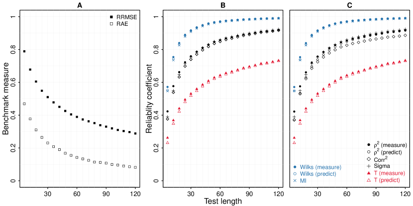
Figure 2: Two benchmark measures (panel A) and relability measures (panels B and C) as functions of test length. Latent scores are original LVs in panel B, and are percentile ranks of LVs in panel C. RRMSE = root relative mean squared error in latent variable scores, RAE = relative absolute error in inter-latent-variable correlation, measure = observed score as outcome, predict = latent score as outcome, $\varrho^{2}$ = coefficient of determination ($varrho^{2}$ (measure) = CTT reliability and $varrho^{2}$(predict = PRMSE), $\hbox{Corr}^{2}$ = squared Pearson correlation, sigma = rescaled coefficient sigma (Equation 7), $T$ = coefficient $T$ (Equation 11), MI = rescaled mutual information (Equation 10), and Wilks = one minus Wilks’ lambda.

Figure 2 presents a graphical summary of the numerical results. With increasing test length $m$, the two benchmark measures of estimation error (PRMSE and RAE) monotonically decrease (see Figure 2A), indicating better recovery of LV scores and inter-LV correlations. Although we place PRMSE and RAE within the same plot in which numerical values fall within the unit interval, these values are not directly comparable because they quantify different aspects of the estimates. The RAE is a scalar-valued measure about the inter-LV correlation (ranging from .08 to .47) and RRMSE is a measure for multiple random quantities (i.e., two-dimensional LVs; ranging from .29 to .79).

In Figure 2B, reliability coefficients increase in value as test length $m$ increases, indicating that EAP scores become better proxies of LVs. Different association measures are not always comparable even though they have been normalized because different reliability coefficients are defined for potentially different pairs of observed and latent scores while quantifying distinct forms of association (see Table 1). Figure 2B suggests that the nine reliability coefficients cluster into three groups (shown in different colors). Coefficients of determination (corresponding to CTT reliabliity and PRMSE) together with the rescaled coefficient sigma, are very similar in value across all levels of $m$ (approximately from 0.4 to 0.9). The squared correlation coincides with PRMSE in the population; hence, the estimated the squared correlation and PRMSE exhibit almost identical values in the simulation. CTT reliability is observed to be at least as large as PRMSE, which is a known result (kim.2012, Equation 31). Rescaled sigma lies between CTT reliability and PRMSE when $m$ is small and becomes the largest among the three reliability indexes when $m$ is large. The measurement and prediction versions of coefficient $T$ take on smaller values compared to the coefficients of determination and rescaled sigma. Coefficient $T$ for the measurement decomposition (ranging from .26 to .73) is slightly larger than the coefficient for the prediction decomposition (ranging from .23 to .73), especially at smaller $m$. Finally, the three association measures between the two-dimensional LVs and the two-dimensional EAP scores are the largest in magnitude at all levels of $m$ (approximately ranging .55 and .99). One minus Wilks’ lambdas for generalized measurement decompositions are uniformly larger than those form generalized prediction decompositions, which are in turn uniformly larger than rescaled mutual information.

Transforming LVs to their percentile ranks leaves most coefficients under investigation intact. However, transforming the LVs changes the squared correlation, coefficient of determination based on the prediction decomposition of $\xi_{1}(\underline{\boldsymbol{\eta}})$, and one minus Wilks’ lambda based on the generalized prediction decomposition of $\boldsymbol{\xi}(\underline{\boldsymbol{\eta}})$. In Figure 2C, the squared correlation and the prediction $\varrho^{2}$ are lower than their values in Figure 2B; moreover, the transformation destroys the equivalence between the two coefficients. The prediction decomposition of one-minus Wilks’ lambdas was observed to slightly decrease because of the LV transformation (see Figure 2B versus 2C).

Summary and Discussion

Reliability is a measure of how closely observed and latent scores align with each other. Based on the regression framework of reliability liu.pek&maydeu-olivares.2024; mcdonald.2011, which assumes a LV measurement model, we have shown that reliability can be broadly defined as a measure of association between observed and latent scores (Equation 5). This broad definition subsumes popular indices of reliability such as coefficients of determination such as CTT reliability lord&novick.1968 and PRMSE haberman&sinharay.2010. Because this broad definition of reliability includes very many reliability indices, we identified and described four desiderata that might aid the analyst in selecting the best reliability coefficient(s) for their research. We consider the desiderata of estimability and normalization essential for interpretation. The desiderata of symmetry and invariance, however, are optional depending on the research context.

From our numerical example, we show that different reliability coefficients can be computed from a single measurement model. In general, values of these association measures of reliability increase as a function of test length. Furthermore, reliability measures of association between multiple outcome and explanatory variables (e.g., mutual information and Wilks’ lambda) tend to have larger values compared to reliability measures of association based on univariate regression (e.g., CTT reliability and PRMSE). Importantly, these values of reliability cannot be compared with one another, despite being normalized onto $[0,1]$, because they measure qualitatively distinct associations between latent and observed scores.

Our general framework of reliability expands the notion of reliability in the context of a LV measurement model in several ways. First, the analyst is not constrained by the choice of observed score and latent score to include in a regression. Second, the analyst can choose any association measure beyond the coefficient of determination. Third, the analyst might move from a univariate regression model (e.g., CTT reliability and PRMSE) to a multivariate regression model (e.g., one minus Wilk’s lambda). Fourth, reliability coefficients can further be chosen based on symmetry and transformation invariance. Because some reliability coefficients we have described are relatively unfamiliar, future research should study their performance in real-data and simulation settings (e.g., under different LV measurement models). Furthermore, to encourage the application of these novel reliability coefficients by substantive researchers, methodologists would need to develop benchmarks or recommendations on how these distinct measures of reliability might be qualitatively interpreted. It is our hope that this general framework might motivate the development of novel reliability coefficients that are useful to substantive researchers, which have yet to be incorporated in the current work.