Gradient directions and relative inexactness in optimization and machine learning

Abstract

In this paper, we investigate the influence of noise giving an estimate of the gradient having a acute angle with the original. Noise amplitude has a relative model. The work offers both theoretical calculations and theorems, as well as experimental results. Classic machine learning problems were chosen as experiments - linear and logistic regression, computer vision and natural language processing.

1 Introduction

We consider global optimization problem:

$$\min\limits_{x\in\mathbb{R}^{n}}f(x).$$ (1)

We define $f^{*}$ - as minimum value of $f$ or solution for problem 1 and $x^{*}$: $f(x^{*})=f^{*}$, also for iterative methods with starting point $x^{0}$ we can define $R=\|x^{0}-x^{*}\|_{2}$. We assume that the objective $f$ is $L$-smooth i.e., for all $x,y\in\mathbb{R}^{n}$:

$$\begin{gathered}\|\nabla f(y)-\nabla f(x)\|_{2}\leqslant L\|y-x\|_{2},\\ \text{Or equivalent and more usefull:},\\ f(y)\leqslant f(x)+\langle\nabla{f}(x),y-x\rangle+\frac{L}{2}\|x-y\|_{2}^{2}\end{gathered}$$ (2)

Also we consider stochastic optimization:

$$\begin{gathered}f(x)\to\min\limits_{x\in\mathbb{R}^{n}},\\ \mathbb{E}\left[\widetilde{\nabla}{f}(x)|x\right]=\nabla f(x).\end{gathered}$$ (3)

The classical formulation of the machine learning problem is the sum-structured problem:

$$f(\theta)=\frac{1}{m}\sum\limits_{i=1}^{m}f_{i}(\theta)\to\min\limits_{\theta\in\mathbb{R}^{n}}.$$ (4)

Here $\theta$ - model parameters and $f_{i}$ - loss function on sample $i$. Stochastic optimization in this problem is defined as follows:

$$\begin{gathered}I\sim\mathcal{U}\{1\dots m\}\times\dots\times\mathcal{U}\{1\dots m\},\\ \widetilde{f}(\theta)=\frac{1}{B}\sum\limits_{i\in I}f_{i}(\theta).\end{gathered}$$

Where $B$ - batch size. We introduce two model errors in gradient:

$$\|\tilde{\nabla}f(x)-\nabla f(x)\|_{2}\leqslant\delta,\text{ (absolute error) or }$$ (5)

$$\|\tilde{\nabla}f(x)-\nabla f(x)\|_{2}\leqslant\alpha\|\nabla f(x)\|_{2},\text{ (relative error)}.$$ (6)

For 6 model we will use the following condition:

$$(\forall x\in\mathbb{R}^{n}):\;\langle\widetilde{\nabla}f(x),\nabla f(x)\rangle\geqslant\gamma\|\widetilde{\nabla}f(x)\|_{2}\|\nabla{f}(x)\|_{2},\quad\gamma\in(0,1]$$ (7)

We can interpret the condition 7 as lower bound for cosine angle between gradient and it is estimation. Follow [15, 2] we can define $(\nu,\rho)$ – noise growth condition:

$$(\forall x\in\mathbb{R}^{n}):\;\nu\|\nabla f(x)\|_{2}\leqslant\|\widetilde{\nabla}f(x)\|_{2}\leqslant\rho\|\nabla{f}(x)\|_{2}$$ (8)

We can note, that relative model 6 with $\alpha\in[0;1)$ implies 7 and growth model 8 with:

$$\gamma=\sqrt{1-\alpha^{2}},\\ \nu=1-\alpha,\\ \rho=1+\alpha.$$ (9)

We propose studies of the convergence of first-order methods with conditions 2, 7, 8. We will prove, that classic gradient procedure 1 will preserves the order of convergence up to constants:

$$f(x^{N})-f^{*}=O\left(\frac{\rho^{2}}{\nu^{2}\gamma^{2}}\frac{LR^{2}}{N}\right)$$

In Sections 5, 6 provided motivation and relevant to [10], [6] results, associated with $\sqrt{\frac{\mu}{L}}$, where $\mu$ - constant of strong convexity 14.

Paper contains a sufficient number of experiments with modern deep learning models with coefficients $\alpha,\gamma$ estimation. Sufficient conditions for the dataset are also given that guarantee the conditions 6, 7.

2 Ideas behind the results

Most papers consider absolute model 5, but what $\delta$ should we choose for theoretical estimation of convergence. For example Algorithm 1 has convergence (for convex function with 2):

$$f(x^{N})-f^{*}=O\left(\frac{LR^{2}}{N}+\delta\right).$$

If estimation for $\delta$ is large the theoretical convergence will be uninformative, but if we plot convergence plot we will see decreasing graph. As an example we can take dataset CIFAR-10 [11] for classification problem. Dataset consist of 50k training samples and 10k test samples of 32x32 images with 10 classes. We will use ResNet-18 [8] as classification model and PyTorch framework [12], because it provides batching. We will estimate $\alpha,\delta$ and $\gamma$ coefficient on each iteration by transforming epochs to iterations. Iterate over all batches (dataloader in PyTorch) we can summarize gradients per batches to gradient for whole train dataset, then choosing single batch we can evaluate required values.

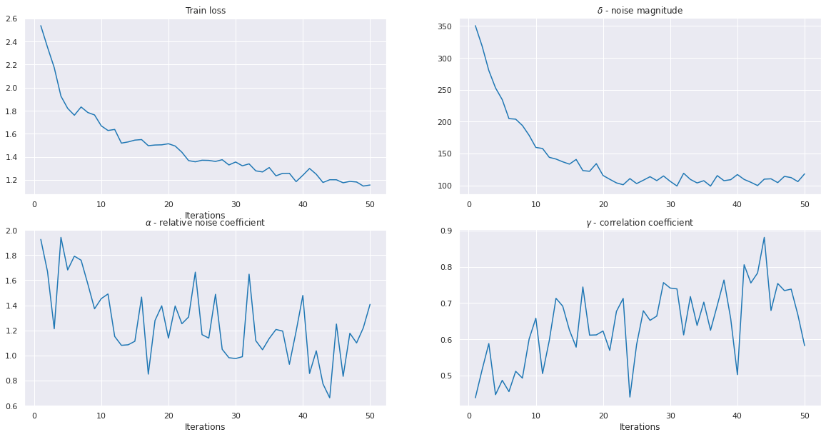
Figure 1: Convergence and coefficient evaluation per iterations for ResNet-18 CIFAR-10.

We can see, that $\gamma$ - 0.45, gives intuition to explore convergence with such conditions. More experiments provided at Section 8. We should note, that for stochastic optimization 3 convergence can be much better, using only $\delta_{*}=\mathbb{E}\|\widetilde{\nabla}f(x^{*})\|_{2}$, more details at [16].

3 Motivation for relative noise

Most works consider an absolute noise model 5, for example  [4, 1, 5]. However there are many papers consider relative model 6 - [6, 15, 10, 14]. These noise models can be approached from the point of view of stochastic differential equations, since the origin of the standard gradient procedure can be perceived as a discretization corresponding to an autonomous system. For models 5, 6, consider the following autonomous SDEs, respectively.

$$dX_{t}=-\nabla{f}(X_{t})dt+\delta\cdot dW_{t},$$ (10)

$$dX_{t}=-\nabla{f}(X_{t})dt+\alpha\|\nabla{f}(X_{t})\|_{2}\cdot dW_{t}.$$ (11)

For SDE:

$$dX_{t}=b(X_{t})dt+\Sigma(X_{t})dW_{t},$$

we can define infinitesimal operator:

$$\mathcal{A}\phi=L_{b}\phi+\frac{1}{2}tr\left(\Sigma\Sigma^{T}\frac{\partial^{2}\phi}{\partial x^{2}}\right),\quad L_{b}\phi=\langle b(x),\nabla\phi(x)\rangle.$$ (12)

One can show:

$$\mathcal{A}^{*}\phi=-div(b\cdot\phi)+\frac{1}{2}\sum\limits_{i,j}\partial_{x_{i},x_{j}}D_{i,j}\phi,\quad D(x)=\Sigma(x)\Sigma^{T}(x).$$

For the distribution solution of the stochastic differential equation, the Fokker-Planck equation is valid:

$$\partial_{t}P=\mathcal{A}^{*}P.$$ (13)

According to [17] stationary solution of Fokker-Planck equation 13 for 10:

$$p^{*}(x)\propto\exp\left({-\frac{2f(x)}{\delta^{2}}}\right).$$

Where $P$ is probability measure and $p^{*}$ - density of this measure (if it exists). For equation 11 we can obtain:

$$\mathcal{A}_{\alpha}\phi=L_{-\nabla{f}}\phi+\frac{\alpha^{2}}{2}\|\nabla{f}\|_{2}^{2}\mathop{}\!\mathbin{\bigtriangleup}{\phi}.$$

We will look for a stationary solution to the Fokker-Planck equation for the equation 11:

$$\forall\phi\in C_{0}^{\infty}\left(\mathbb{R}^{n}\right)\int_{\mathbb{R}^{n}}\left(\mathcal{A}_{\alpha}\phi\right)P^{*}(dx)=0.$$

We can note, that any distribution $P^{*}$ concentrated on $X^{*}=\{x\;|\;\nabla{f}(x)=0\}$ will be solution. Thus, assuming a model 6, we can expect same convergence as for models without noise. Note, that 11 does not assume $\alpha<1$, this effect will be noted in Section 5.

4 Gradient descent

In this section, we consider problem 1. We will use conditions 5 and 7. Let us introduce classic procedure

Algorithm 1 Gradient Descent $(h,x^{0})$

1:Input: Starting point $x^{0}$, number of steps $N$, $h$ - learning rate.

2:for $k=1\dots N$ do

3:     $x^{k}=x^{k-1}-h\widetilde{\nabla}f(x^{k-1})$

4:end for

5:Output: $x^{N}$.

Lemma 4.1.

Let $f$ function satisfies condition 2, and $\widetilde{\nabla}f$ satisfies 8 and 7. Then Algorithm 1 with $h<\frac{2\nu\gamma}{L\rho^{2}}$ produce:

$$\|\nabla f(x^{k})\|_{2}^{2}\leqslant\tau\left(f(x^{k})-f(x^{k+1})\right)$$

Where:

$$\tau^{-1}=h\left(\nu\gamma-\frac{Lh\rho^{2}}{2}\right)$$

Proof.

$$\begin{gathered}f(x^{k+1})\leqslant f(x^{k})+\langle\nabla{f}(x^{k}),x^{k+1}-x^{k}\rangle+\frac{L}{2}\|x^{k+1}-x^{k}\|_{2}^{2},\\ f(x^{k+1})\leqslant f(x^{k})+\langle\nabla{f}(x^{k}),-h\widetilde{\nabla}f(x^{k})\rangle+\frac{h^{2}L}{2}\|\widetilde{\nabla}f(x^{k})\|_{2}^{2},\\ f(x^{k+1})\leqslant f(x^{k})-h\nu\gamma\|\nabla{f}(x^{k})\|_{2}^{2}+\frac{h^{2}L\rho^{2}}{2}\|\nabla{f}(x^{k})\|_{2}^{2}\end{gathered}$$

Then we obtain desired inequality. ∎

Lemma 4.2.

Let $f$ function satisfies conditions Lemma 4.1, then:

$$\|x^{k}-x^{*}\|_{2}^{2}\leqslant 2\left(Lh^{2}\rho^{2}\tau+1\right)R^{2}$$

Proof.

Using Lemma 4.1 and telescopic sum:

$$\begin{gathered}\|x^{k}-x^{*}\|_{2}^{2}\leqslant 2\|x^{k}-x^{0}\|_{2}^{2}+2\|x^{0}-x^{*}\|_{2}^{2},\\ \|x^{k}-x^{0}\|_{2}^{2}\leqslant\|h\sum_{j=0}^{k-1}\widetilde{\nabla}f(x^{j})\|_{2}^{2}\leqslant 2h^{2}\rho^{2}\sum_{j=0}^{k-1}\|\nabla f(x^{j})\|_{2}^{2}\leqslant 2h^{2}\rho^{2}\tau\Delta_{0}\leqslant Lh^{2}\rho^{2}\tau R^{2},\\ \|x^{k}-x^{*}\|_{2}^{2}\leqslant 2\left(Lh^{2}\rho^{2}\tau+1\right)R^{2}\end{gathered}$$

∎

Theorem 4.3.

Let $f$ - convex function and satisfies condition 2, and $\widetilde{\nabla}f$ satisfies 8 and 7 then Algorithm 1. Then with $h<\frac{2\nu\gamma}{L\rho^{2}}$ we obtain:

$$\begin{gathered}f(x^{N})-f^{*}\leqslant\frac{2\left(Lh^{2}\rho^{2}\tau+1\right)}{h\left(\nu\gamma-\frac{Lh\rho^{2}}{2}\right)}\frac{R^{2}}{N+1},\\ R=\|x^{0}-x^{*}\|_{2},\;\tau^{-1}=h\left(\nu\gamma-\frac{Lh\rho^{2}}{2}\right)\end{gathered}$$

Proof.

Let us define: $\Delta_{k}=f(x^{k})-f^{*}$. Using convexity of function $f$ and Cauchy Bunyakovsky Schwarz inequality we obtain:

$$\begin{gathered}f(x^{k})+\langle\nabla{f}(x^{k}),x^{*}-x^{k}\rangle\leqslant f^{*},\\ \Delta_{k}\leqslant\|\nabla f(x^{k})\|_{2}\|x^{k}-x^{*}\|_{2}\end{gathered}$$

Let us define $\lambda=2\left(Lh^{2}\rho^{2}\tau+1\right)$. Using Lemma 4.1 and Lemma 4.2:

$$\begin{gathered}\|\nabla f(x^{k})\|_{2}^{2}\geqslant\frac{\Delta_{k}}{\lambda R^{2}},\\ \Delta_{k+1}\leqslant\Delta_{k}-\frac{1}{\lambda\tau R^{2}}\Delta_{k}^{2}.\end{gathered}$$

Then, using previous relation we will prove by induction convergence rate: Base $N=2$, because $\tau$ minimum takes place with $h=\frac{\nu\gamma}{L\rho^{2}}$:

$$\begin{gathered}f(x^{2})\leqslant f^{*}+\frac{L}{2}\|x^{2}-x^{*}\|_{2}^{2},\\ \Delta_{2}\leqslant\frac{\lambda LR^{2}}{2}<\frac{2\lambda LR^{2}}{3}\leqslant\frac{\lambda\tau R^{2}}{3}\end{gathered}$$

Step $N+1>2$:

$$\begin{gathered}\text{Assume: }\Delta_{N}\leqslant\frac{\lambda\tau R^{2}}{N+1},\\ \text{If: }\Delta_{N}\leqslant\frac{\lambda\tau R^{2}}{N+2}\Rightarrow\Delta_{N+1}\leqslant\frac{\lambda\tau R^{2}}{N+2},\\ \text{If: }\Delta_{N}>\frac{\lambda\tau R^{2}}{N+2},\\ \text{Function: }g(x)=\frac{1}{x}-\frac{1}{x^{2}}\text{ - decreasing for }x>2,\\ \frac{\lambda\tau R^{2}}{N+1}-\frac{\lambda\tau R^{2}}{(N+1)^{2}}<\frac{\lambda\tau R^{2}}{N+2}\Rightarrow\Delta_{N+1}\leqslant\frac{\lambda\tau R^{2}}{N+2}\end{gathered}$$

Thus we obtain convergence. ∎

Theorem 4.4.

Let $f$ - function and satisfies condition 2, $\widetilde{\nabla}f$ satisfies 8 and 7 then procedure 1. Then with $h<\frac{2\nu\gamma}{L\rho^{2}}$ we obtain:

$$\min_{0\leqslant k\leqslant N}\|\nabla{f}(x^{k})\|_{2}^{2}\leqslant\frac{f(x^{0})-f^{*}}{h\left(\nu\gamma-\frac{Lh\rho^{2}}{2}\right)\left(N+1\right)}.$$

Proof.

Using Lemma 4.1 and summarize it from $0$ to $N$:

$$\begin{gathered}\sum_{j=0}^{N}\|\nabla{f}(x^{j})\|_{2}^{2}\leqslant\tau\sum_{j=0}^{N}\left(f(x^{j})-f(x^{j+1})\right)=\tau\left(f(x^{0})-f(x^{N+1})\right)\leqslant\tau\left(f(x^{0})-f^{*}\right),\\ (N+1)\min_{0\leqslant k\leqslant N}\|\nabla{f}(x^{k})\|_{2}^{2}\leqslant\tau\left(f(x^{0})-f^{*}\right),\\ \min_{0\leqslant k\leqslant N}\|\nabla{f}(x^{k})\|_{2}^{2}\leqslant\frac{\tau\left(f(x^{0})-f^{*}\right)}{N+1}.\end{gathered}$$

∎

Remark 4.1.

In conditions of Theorem 4.3 we can choice

$$h=\frac{\nu\gamma}{L\rho^{2}}.$$

Then:

$$\begin{gathered}\tau=\frac{2L\rho^{2}}{\nu^{2}\gamma^{2}},\\ \lambda=2\left(Lh^{2}\rho^{2}\tau+1\right)=6,\\ f(x^{N})-f^{*}\leqslant\frac{12L\rho^{2}R^{2}}{\nu^{2}\gamma^{2}(N+1)}=O\left(\frac{\rho^{2}}{\nu^{2}\gamma^{2}}\frac{LR^{2}}{N+1}\right),\\ \min_{0\leqslant k\leqslant N}\|\nabla{f}(x^{k})\|_{2}^{2}\leqslant\frac{\rho^{2}}{\nu^{2}\gamma^{2}}\frac{2L\left(f(x^{0})-f^{*}\right)}{N+1}.\end{gathered}$$

Theorem 4.5.

Let $f$ - function and satisfies condition 2, and $\widetilde{\nabla}f$ satisfies 6 then Algorithm 1 with

$$h=\left(\frac{1-\alpha}{1+\alpha}\right)^{\frac{3}{2}}\frac{1}{L},$$

has convergence:

$$\begin{gathered}f(x^{N})-f^{*}\leqslant\frac{12L(1+\alpha)R^{2}}{(1-\alpha)^{3}(N+1)}=O\left(\frac{1+\alpha}{(1-\alpha)^{3}}\frac{LR^{2}}{N+1}\right),\\ \min_{0\leqslant k\leqslant N}\|\nabla{f}(x^{k})\|_{2}^{2}\leqslant\frac{1+\alpha}{(1-\alpha)^{3}}\frac{2L\left(f(x^{0})-f^{*}\right)}{N+1}.\end{gathered}$$

Proof.

Continuing Remark 4.1 and note 9 we obtain theorem above. ∎

Remark 4.2.

We provide not default proof for gradient descent convergence. The reason for this may be the Lyapunov function tool for a dynamic system:

$$\dot{x}=-\widetilde{\nabla}f(x).$$

Function $f$ - will be Lyapunov function for system above, if $\widetilde{\nabla}f$ satisfies condition 7. However $\|x-x^{*}\|_{2}^{2}$ will not:

$$\begin{gathered}L_{\widetilde{\nabla}f}f=-\langle\widetilde{\nabla}f(x),\nabla{f}(x)\rangle\leqslant-\gamma\|\widetilde{\nabla}f(x)\|_{2}\|\nabla{f}(x)\|_{2}<0,\\ L_{\widetilde{\nabla}f}\|x-x^{*}\|_{2}^{2}=-\langle\widetilde{\nabla}f(x),x-x^{*}\rangle\Rightarrow\text{sign of this product is ambiguous }.\end{gathered}$$

5 Similar triangle methods and stochastic optimization

For constrained optimization with set $Q$ we can provide such method:

Algorithm 2 STM $(L,x_{start})$, $Q\subseteq\mathbb{R}^{n}$

1:Input: Starting point $x_{start}$, number of steps $N$.

2:Set $\tilde{x}^{0}=x_{start}$, $\alpha_{0}=\frac{1}{L}$, $A_{0}=\frac{1}{L}$.

3:Set $\psi_{0}(x)=\frac{1}{2}\|x-\tilde{x}^{0}\|_{2}^{2}+\alpha_{0}\left(f(\tilde{x}^{0})+\langle\tilde{\nabla}f(\tilde{x}^{0}),x-\tilde{x}^{0}\rangle\right)$.

4:Set $z_{0}=\mathop{\arg\!\min}_{y\in Q}{\psi_{0}(y)}$, $x^{0}=z^{0}$.

5:for $k=1\dots N$ do

6:     Find $\alpha_{k}$ from $(1+A_{k-1})(A_{k-1}+\alpha_{k})=L\alpha_{k}^{2}$,

7:

8:     or equivalently $\alpha_{k}=\frac{1}{2L}+\sqrt{\frac{1}{4L^{2}}+\frac{A_{k-1}}{L}}$,

9:     $A_{k}=A_{k-1}+\alpha_{k},$

10:     $\tilde{x}^{k}=\frac{A_{k-1}x^{k-1}+\alpha_{k}z^{k-1}}{A_{k}},$

11:     $\psi_{k}(x)=\psi_{k-1}(x)+\alpha_{k}\left(f(\tilde{x}^{k})+\langle\widetilde{\nabla}f(\tilde{x}^{k}),x-\tilde{x}^{k}\rangle\right),$

12:     $z^{k}=\mathop{\arg\!\min}_{y\in Q}\psi_{k}(y),$

13:     $x^{k}=\frac{A_{k-1}x^{k-1}+\alpha_{k}z^{k}}{A_{k}}.$

14:end for

15:Output: $x_{N}$.

For not constrained optimization we can rewrite it as implicit method.

Algorithm 3 STM (implicit) $(L,x_{start})$

1:Input: Starting point $x_{start}$, number of steps $N$.

2:Set $y^{0}=x_{start}$, $\alpha_{0}=\frac{1}{L}$, $A_{0}=\frac{1}{L}$.

3:Set $z_{0}=y^{0}-\alpha_{0}\widetilde{\nabla}f(y^{0})$, $x^{0}=z^{0}$.

4:for $k=1\dots N$ do

5:     $\alpha_{k}=\frac{1}{2L}+\sqrt{\frac{1}{4L^{2}}+\frac{A_{k-1}}{L}}$,

6:     $A_{k}=A_{k-1}+\alpha_{k},$

7:     $y^{k}=\frac{A_{k-1}x^{k-1}+\alpha_{k}z^{k-1}}{A_{k}},$

8:     $z^{k}=z^{k-1}-\alpha_{k}\widetilde{\nabla}f(y^{k})$

9:     $x^{k}=y^{k}-\frac{1}{L}\widetilde{\nabla}f(y^{k})$

10:end for

11:Output: $x_{N}$.

5.1 Stochastic optimization

In this section we will consider stochastic optimization:

$$\mathbb{E}_{\xi}\widetilde{\nabla}f(x,\xi)=\nabla{f}(x).$$

With analogue growth condition:

$$\mathbb{E}_{\xi}\|\widetilde{\nabla}f(x,\xi)\|_{2}^{2}\leqslant\kappa\|\nabla f(x)\|_{2}^{2}.$$

In paper [15], Theorem 2 was proved about the convergence of a method similar to  3 with step correction:

$$\mathbb{E}f(x^{N})-f^{*}\leqslant\frac{2\kappa^{2}L}{N^{2}}\|x^{N}-x^{*}\|_{2}^{2}.$$

The condition of unbiased gradient turned out to be very important in the proof of this theorem. First of all it is easy to get lower bound of growth condition 8:

$$\mathbb{E}\|\widetilde{\nabla}f(x,\xi)\|_{2}\geqslant\|\mathbb{E}\widetilde{\nabla}f(x,\xi)\|_{2}=\|\nabla{f}(x)\|_{2}.$$

Gradient direction condition 7 can be interpreted a little differently. We assume that $v$ corresponds to the coordinate $x_{1}$. Define $\mathbb{S}^{n-1}_{v+}$ - top hemisphere for direction $v$. Let us define simple noised gradient model for analysis:

$$\begin{gathered}\mathbb{E}u=v,\\ u\sim\omega\mathcal{U}\left(\mathbb{S}^{n-1}_{v+}\right)+(1-\omega)\mathcal{U}\left(\mathbb{S}^{n-1}_{v-}\right),\;\omega\in[0;1].\end{gathered}$$

Then we can calculate norm of vector $v$, it can be done, because it has only $x_{1}$ non zero coordinate:

$$\begin{gathered}g(n)=\frac{1}{\text{area}\left(\mathbb{S}^{n-1}_{v+}\right)}\int_{\mathbb{S}^{n-1}_{v+}}x_{1}dA,\\ \|v\|_{2}=(2\omega-1)g(n)\Rightarrow\omega=\frac{1}{2}+\frac{\|v\|_{2}}{2g(n)}>\frac{1}{2},\\ P\left(\langle u,v\rangle>0\right)=\omega>\frac{1}{2}.\end{gathered}$$

Then we can move to batching estimation to study direction of batched estimation:

$$\begin{gathered}S_{m}=\frac{1}{m}u_{j},\;u_{j}-\text{i.i.d (batching)},\\ P\left(\langle S_{m},v\rangle>0\right)=P\left(\frac{1}{m}\sum_{k=1}^{m}\cos{\phi_{k}}>0\right),\;\phi_{k}\sim\mathcal{D}_{\omega},\\ \mathcal{D}_{\omega}=\omega\mathcal{U}\left(\left[0;\frac{\pi}{2}\right]\right)+(1-\omega)\mathcal{U}\left(\left[\frac{\pi}{2};\pi\right]\right),\\ a_{\omega}=\mathbb{E}_{\mathcal{D}_{\omega}}\cos{\phi}=\frac{2(2\omega-1)}{\pi},\\ \sigma_{\omega}^{2}=\mathrm{Var}_{\mathcal{D}_{\omega}}\sin{\phi}=\frac{1}{2}-a_{\omega}^{2},\\ P\left(\langle S_{m},v\rangle>0\right)\geqslant 1-P\left(\left|\frac{1}{m}\sum_{k=1}^{m}\cos{\phi_{k}}-a\right|\geqslant a\right)\geqslant 1-\frac{1}{m}\left(\frac{1}{2a_{\omega}^{2}}-1\right),\\ P\left(\langle S_{m},v\rangle>0\right)\geqslant 1-\frac{1}{m}\left(\frac{\pi^{2}}{8(2\omega-1)^{2}}-1\right)=1-\frac{1}{m}\left(\frac{\pi^{2}}{8}\frac{g^{2}(n)}{\|v\|_{2}^{2}}-1\right).\end{gathered}$$

Such model gives us, that unbiased uniformly distributed $\widetilde{\nabla}f(x,\xi)$ gives $P\left(\langle\widetilde{\nabla}f(x,\xi),\nabla f(x)\rangle>0\right)=\omega>\frac{1}{2}$ and using batching this probability can be increased to $1-\frac{1}{m}\left(\frac{\pi^{2}}{8}\frac{1}{(2\omega-1)^{2}}-1\right)$ and we can note as the $\nabla{f}(x)$ norm increases, so does the probability.

5.2 Strongly convex case, not stochastic

We call function $f$ $\mu$-strongly convex, if:

$$(\forall x,y\in\mathbb{R}^{n}):\;f(x)+\langle\nabla{f}(x),y-x\rangle+\frac{\mu}{2}\|x-y\|_{2}^{2}\leqslant f(y)$$ (14)

In [10] convergence of analogue of Algorithm 3 for strongly convex case 14 using restarts:

$$\begin{gathered}N=O\left(\sqrt{\frac{L}{\mu}}\log{\frac{\mu R_{0}^{2}}{\varepsilon}}\right)\Rightarrow f(x^{N})-f^{*}\leqslant\varepsilon,\\ \text{If }\alpha\text{(relative error level)}=O\left(\sqrt{\frac{\mu}{L}}\right)\end{gathered}$$

We can give motivation for $\sqrt{\frac{\mu}{L}}$ bound, which appeared in [10, 6] proofs. Firstly one solid geometry fact:

Lemma 5.1 (Cosine $\mathbb{R}^{3}$ theorem).

Let $OABC$ - tetrahedron, $\alpha=\angle BOC,\beta=\angle AOC,\gamma=\angle AOB,\delta=\angle(AOB,AOC)$, then

$$\cos\alpha=\cos\beta\cos\gamma+\sin\beta\sin\gamma\cos\delta.$$

Lemma 5.2.

We call function $f$ - noised $\beta,\mu$-strongly quasiconvex at points $x,x^{*}$, if:

$$f(x)+\beta^{-1}\langle\widetilde{\nabla}f(x),x^{*}-x\rangle+\frac{\mu}{2}\|x^{*}-x\|_{2}^{2}\leqslant f^{*},\;\beta\in(0;1).$$ (15)

If $f$ - $\mu$-strongly convex 14 and smooth 2, $\widetilde{\nabla}f$ satisfies 6, $\alpha<\sqrt{\frac{\mu}{L}}$, then $f$ satisfies 15 with $\beta=\frac{1}{2}$.

Proof.

As $f$ is convex, then:

$$f(x)+\langle\nabla{f}(x),x^{*}-x\rangle\leqslant f^{*}\Rightarrow\langle\nabla{f}(x),x-x^{*}\rangle\geqslant f(x)-f^{*}.$$

Using $\mu,L$ constants conditions:

$$\langle\nabla{f}(x),x-x^{*}\rangle=\gamma(x)\|\nabla{f}(x)\|_{2}\|x^{*}-x\|_{2}\leqslant 2\gamma(x)\sqrt{\frac{L}{\mu}}\left(f(x)-f^{*}\right).$$

Then we get $\gamma(x)\geqslant\frac{1}{2}\sqrt{\frac{\mu}{L}}$. We can decompose:

$$\widetilde{\nabla}f(x)=\nabla f(x)+r(x),\;\|r(x)\|_{2}\leqslant\alpha\|\nabla f(x)\|_{2}.$$

Let us define $\widetilde{\gamma}(x)$ such as:

$$\left\langle\frac{1}{2}\nabla f(x)+r(x),x-x^{*}\right\rangle=\widetilde{\gamma}(x)\left\|\frac{1}{2}\nabla f(x)+r(x)\right\|_{2}\|x-x^{*}\|_{2}.$$

Using Lemma 5.1:

$$\widetilde{\gamma}(x)\geqslant\frac{1}{2}\sqrt{1-\frac{\alpha^{2}}{4}}\sqrt{\frac{\mu}{L}}-\frac{\alpha}{2}\sqrt{1-\frac{\mu}{4L}}.$$

That is, $\left\langle\frac{1}{2}\nabla{f}(x)+r(x),x-x^{*}\right\rangle\geqslant 0\Longleftrightarrow\alpha<\sqrt{\frac{\mu}{L}}$. Then:

$$f(x)+2\left\langle\nabla{f}(x)+r(x),x^{*}-x\right\rangle+\frac{\mu}{2}\|x^{*}-x\|_{2}^{2}$$

$$=f(x)+\langle\nabla{f}(x),x^{*}-x\rangle+\frac{\mu}{2}\|x^{*}-x\|_{2}^{2}+2\left\langle\frac{1}{2}\nabla{f}(x)+r(x),x^{*}-x\right\rangle$$

$$\leqslant f^{*}.$$

∎

6 Conjugate Gradients

In this section we will provide accelerated method 4 for model 2, 7, 8. We will limit the set of functions to the simplified strong convex condition. We will say, that function $f$ satisfies quadratic growth condition with parameter $\mu$ at point $x$ if:

$$\frac{\mu}{2}\|x-x^{*}\|_{2}^{2}\leqslant f(x)-f^{*}.$$ (16)

This condition was taken from [7] as well as the algorithm 4. We will use this condition to prove analogues of the results from the papers [6, 10, 14].

Algorithm 4 CG $(h,x_{start})$

1:Input: Starting point $x_{start}$, number of steps $N$.

2:Set $u^{0}=0$.

3:Set $y^{0}=0$.

4:for $k=1\dots N$ do

5:     $x^{k}=y^{k-1}-h\widetilde{\nabla}f(y^{k-1})$

6:     $u^{k}=u^{k-1}+\widetilde{\nabla}f(y^{k-1})$

7:     $y^{k}=\mathop{\arg\!\min}\limits_{x=x^{0}+\text{Lin}\{{x^{k}-x^{0},u^{k}\}}}f(x).$

8:end for

9:Output: $x^{N}$.

Theorem 6.1.

Let $f$ - convex function and satisfies condition 2, $\widetilde{\nabla}f$ satisfies 7 and 8, starting point $x^{0}$ satisfies 16, then procedure 1 with $h<\frac{2\nu\gamma}{L\rho^{2}}$ produce:

$$f(x^{N})-f^{*}\leqslant\omega(f(x^{0})-f^{*}),\;\omega=\frac{3}{4}.$$

Where:

$$N>\max\left\{\frac{2}{\omega}\rho\sqrt{\frac{\tau}{\mu}},\frac{4\rho^{2}\sqrt{1-\gamma^{2}}\tau}{\mu\omega^{2}}\right\},\;\tau^{-1}=h\left(\nu\gamma-\frac{Lh\rho^{2}}{2}\right)$$

Proof.

Let’s conduct a proof against the contrary, assume:

$$f(x^{N})-f^{*}\geqslant\omega(f(x^{0})-f^{*}).$$

Using Lemma 4.1 and $f(x^{k})\leqslant f(y^{k})$ we obtain:

$$\|\nabla{f}(y^{k})\|_{2}^{2}\leqslant\tau\left(f(x^{k})-f(x^{k+1})\right)$$

Summing up inequalities above:

$$\sum_{k=0}^{N-1}\|\nabla{f}(y^{k})\|_{2}^{2}\leqslant\tau\left(f(x^{0})-f^{*}\right).$$

From definition of $y^{k}$ and first order condition we obtain:

$$\langle\nabla{f}(y^{k}),x^{k}-x^{0}\rangle=\langle\nabla{f}(y^{k}),u^{k}\rangle=0.$$

Using convexity:

$$\omega(f(x^{0})-f^{*})\leqslant f(y^{k})-f^{*}\leqslant\langle\nabla{f}(y^{k}),x^{*}-y^{k}\rangle=\langle\nabla{f}(y^{k}),x^{*}-x^{0}\rangle.$$

Summing up inequalities above:

$$\omega N(f(x^{0})-f^{*})\leqslant\langle u^{N},x^{*}-x^{0}\rangle.$$

Using condition 7, Lemma 5.1 and $\langle u^{k},\nabla{f}(y^{k})\rangle=0$:

$$\langle\widetilde{\nabla}{f}(y^{k}),u^{k}\rangle\leqslant\sqrt{1-\gamma^{2}}\|\widetilde{\nabla}{f}(y^{k})\|_{2}\|u^{k}\|_{2}.$$

Then:

$$\left\|u^{N}\right\|_{2}^{2} \leqslant\|\widetilde{\nabla}{f}(y^{N-1})\|_{2}^{2}+\|u^{N-1}\|_{2}^{2}+\sqrt{1-\gamma^{2}}\|u^{N-1}\|_{2}\|\widetilde{\nabla}{f}(y^{N-1})\|_{2}$$

$$\leqslant\rho^{2}\|\nabla{f}(y^{N-1})\|_{2}^{2}+\|u^{N-1}\|_{2}^{2}+\sum_{k=0}^{N-2}\rho^{2}\sqrt{1-\gamma^{2}}\left(\|\nabla{f}(y^{k})\|_{2}^{2}+\|\nabla{f}(y^{N-1}\|_{2}^{2}\right)$$

$$\leqslant\rho^{2}\sum_{k=0}^{N-1}\|\nabla{f}(y^{k})\|_{2}^{2}+\rho^{2}\sqrt{1-\gamma^{2}}\sum_{k=0}^{N-1}(N-1)\|\nabla{f}(y^{k})\|_{2}^{2}$$

$$\leqslant\rho^{2}\left(1+\sqrt{1-\gamma^{2}}N\right)\sum_{k=0}^{N-1}\|\nabla{f}(y^{k})\|_{2}^{2}\leqslant 2\rho^{2}\max\{1,\sqrt{1-\gamma^{2}}N\}\tau(f(x^{0})-f^{*})$$

Using quadratic growth at point $x^{0}$:

$$\frac{\mu}{2}\|x^{0}-x^{*}\|_{2}^{2}\leqslant f(x^{0})-f(x^{*}).$$

Then:

$$\begin{gathered}\omega N(f(x^{0})-f^{*})\leqslant\sqrt{\frac{4}{\mu}}\rho\sqrt{\tau\max\{1,\sqrt{1-\gamma^{2}}N\}}(f(x^{0})-f^{*})\Rightarrow\\ \Rightarrow N\leqslant\max\left\{\frac{2}{\omega}\rho\sqrt{\frac{\tau}{\mu}},\frac{4\rho^{2}\sqrt{1-\gamma^{2}}\tau}{\mu\omega^{2}}\right\}\end{gathered}$$

This ends the proof. ∎

Theorem 6.2.

Let $f$ - function and satisfies condition 2, $\widetilde{\nabla}f$ satisfies 6 and $x^{0}$ satisfies 16 then procedure 4 with

$$h=\left(\frac{1-\alpha}{1+\alpha}\right)^{\frac{3}{2}}\frac{1}{L},$$

and:

$$\alpha<\sqrt{\frac{\mu}{L}}.$$

produce:

$$\begin{gathered}f(x^{N})-f^{*}\leqslant\frac{3}{4}(f(x^{0})-f^{*}),\\ N>\frac{64\left(1+\alpha\right)^{3}}{9\left(1-\alpha\right)^{3}}\sqrt{\frac{L}{\mu}}.\end{gathered}$$

Proof.

Using Theorem 6.1 and defined step $h$ we obtain the result. We should note, that

$$\frac{\left(1+\alpha\right)^{3}}{\left(1-\alpha\right)^{3}}=O\left(1\right).$$

∎

Theorem 6.2 allows us to obtain an accelerated method that preserves convergence under conditions of relative noise with $\alpha=O\left(\sqrt{\frac{\mu}{L}}\right)$. This result corresponds papers [6, 10]. The disadvantage of this approach is the need to use the oracle of low-dimensional optimization.

7 Sufficient conditions for datasets

7.1 Logistic regression

In this section we will provide some sufficient conditions for 7, 8. Consider sum-structured optimization problem 4 with dataset $\mathcal{D}=\{(x_{k},y_{k})\}_{k=1}^{M}$, where $x_{k}$ - features of object $k$ and $y_{k}\in\{0,1\}$ - object‘s class, for model we consider logistic regression for simplicity:

$$\begin{gathered}\sigma(x)=\frac{1}{1+e^{-x}},\\ f_{k}(\theta)=y_{k}\ln\sigma\left(x_{k}^{T}\theta\right)+(1-y_{k})\ln\left(1-\sigma\left(x_{k}^{T}\theta\right)\right),\\ f(\theta)=\frac{1}{M}\sum_{j=1}^{M}f_{k}(\theta),\\ u_{k}(\theta)=\nabla f_{k}(\theta)=x_{k}\left(y_{k}\left(1-\sigma\left(x_{k}^{T}\theta\right)\right)-(1-y_{k})\sigma\left(x_{k}^{T}\theta\right)\right).\end{gathered}$$ (17)

We define features consistency property for dataset $\mathcal{D}$:

$$\begin{gathered}(\exists\Upsilon\in(0;1])(\forall i,k\in\{1\dots M\}),\\ y_{i}=y_{k}\Rightarrow\langle x_{i},x_{k}\rangle\geqslant\Upsilon\|x_{i}\|_{2}\|x_{k}\|_{2},\\ y_{i}\not=y_{k}\Rightarrow\langle x_{i},x_{k}\rangle\leqslant-\Upsilon\|x_{i}\|_{2}\|x_{k}\|_{2},\\ \end{gathered}$$ (18)

Theorem 7.1.

If dataset $\mathcal{D}$ satisfies features consistency 18 then single element gradient estimation satisfies condition 7.

Proof.

Let $\widetilde{\nabla}f(x)=u_{\xi}(x)$, $\xi\in\{1\dots M\}$.

$$\begin{gathered}\langle u_{\xi}(\theta),\frac{1}{M}\sum_{j=1}^{M}u_{k}(\theta)\rangle=\frac{1}{M}\sum_{k=1}^{M}\langle u_{\xi}(\theta),u_{k}(\theta)\rangle,\\ y_{\xi}=y_{k}=1\Rightarrow\langle u_{\xi}(\theta),u_{k}(\theta)\rangle=\langle x_{\xi},x_{k}\rangle\left(1-\sigma\left(x_{\xi}^{T}\theta\right)\right)\left(1-\sigma\left(x_{k}^{T}\theta\right)\right),\\ y_{\xi}=1,y_{k}=0\Rightarrow\langle u_{\xi}(\theta),u_{k}(\theta)\rangle=-\langle x_{\xi},x_{k}\rangle\left(1-\sigma\left(x_{\xi}^{T}\theta\right)\right)\sigma\left(x_{k}^{T}\theta\right)\geqslant\Upsilon\|u_{\xi}(\theta)\|_{2}\|u_{k}(\theta)\|_{2},\\ \text{Analogically for }y_{\xi}=y_{k}=0,\\ \frac{1}{M}\sum_{k=1}^{M}\langle u_{\xi}(\theta),u_{k}(\theta)\rangle\geqslant\Upsilon\|u_{\xi}(\theta)\|_{2}\bigg{\|}\frac{1}{M}\sum_{k=1}^{M}u_{k}(\theta)\bigg{\|}_{2},\\ \Rightarrow\langle\widetilde{\nabla}f(x),\nabla f(x)\rangle\geqslant\Upsilon\|\widetilde{\nabla}f(x)\|_{2}\|\nabla f(x)\|_{2}.\end{gathered}$$

∎

Theorem 7.2.

If dataset $\mathcal{D}$ satisfies features consistency 18 then batch gradient estimation satisfies condition 7.

Proof.

Using linearity of scalar product and Theorem 7.1 easy to obtain theorem. ∎

7.2 Linear inverse problem

Consider a system of linear equations with respect to $\theta$:

$$X\theta=Y,\;X\in\mathrm{GL}_{m}(\mathbb{R})-\text{invertable matrix},\;Y\in\mathbb{R}^{m}.$$ (19)

We can map the convex optimization problem to a system 19:

$$f(\theta)=\frac{1}{2m}\|X\theta-Y\|_{2}^{2}=\frac{1}{2m}\sum_{k=1}^{m}(x_{k}^{T}\theta-y_{k})^{2}.$$ (20)

Since the matrix is non-generated, then $\exists\theta^{*}:\;X\theta^{*}=Y$, then:

$$\begin{gathered}\nabla f(\theta)=\frac{1}{m}\sum_{k=1}^{m}P_{k}\Delta\theta,\\ \Delta\theta=\theta-\theta^{*},\\ P_{k}=x_{k}x_{k}^{T},\\ S=\frac{1}{m}\sum_{k=1}^{m}P_{k}.\end{gathered}$$

Theorem 7.3.

If matrix $X\in\mathrm{GL}_{m}(\mathbb{R})$ and satisfies:

$$\forall j,k:\;1\leqslant j,k\leqslant m:\;\langle x_{k},x_{j}\rangle\geqslant\Upsilon\|x_{k}\|_{2}\|x_{j}\|_{2}.$$

Then single element gradient estimation $\widetilde{\nabla}f(\theta)=P_{\xi}\Delta\theta$ satisfies 7.

Proof.

$$\langle\nabla f(\theta),\widetilde{\nabla}f(\theta)\rangle =\langle S\Delta\theta,P_{\xi}\Delta\theta\rangle=\frac{1}{m}\sum_{k=1}^{m}\langle P_{k}\Delta\theta,P_{\xi}\Delta\theta\rangle\geqslant$$

$$\Upsilon\frac{1}{m}\sum_{k=1}^{m}\|P_{k}\Delta\theta\|_{2}\|P_{\xi}\Delta\theta\|_{2}\geqslant\Upsilon\|S\Delta\theta\|_{2}\|P_{\xi}\Delta\theta\|_{2}.$$

∎

Unfortunately using batching we can not provide gradient estimations satisfying condition 8, because $P_{k}\Delta\theta$ can equals $0$ for some $k$.

8 Numerical experiments

In this section we provide several experiments with an example of real deep learning problems with parameter estimation from definitions 5, 6, 7. We will use Adam optimization algorithm [9].

8.1 Computer Vision

Firstly we examine ResNet18 [8]:

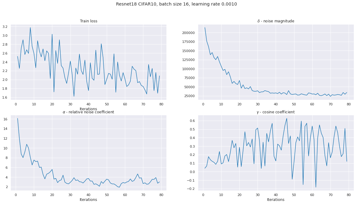
Figure 2: ResNet-18 CIFAR-10 batch size - 16

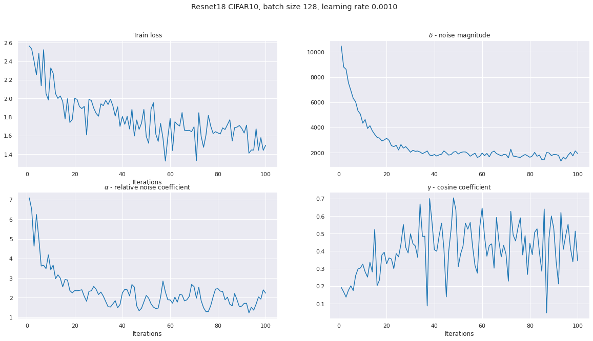
Figure 3: ResNet-18 CIFAR-10 batch size - 128

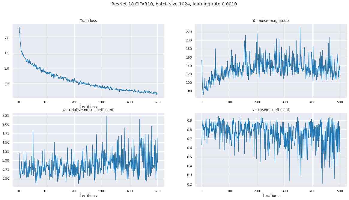
Figure 4: ResNet-18 CIFAR-10 batch size - 1024

8.2 Natural Language Processing

Let us examine NLP classification problem on AG News dataset [18]. Firstly consider LSTM [13] with 3 layers:

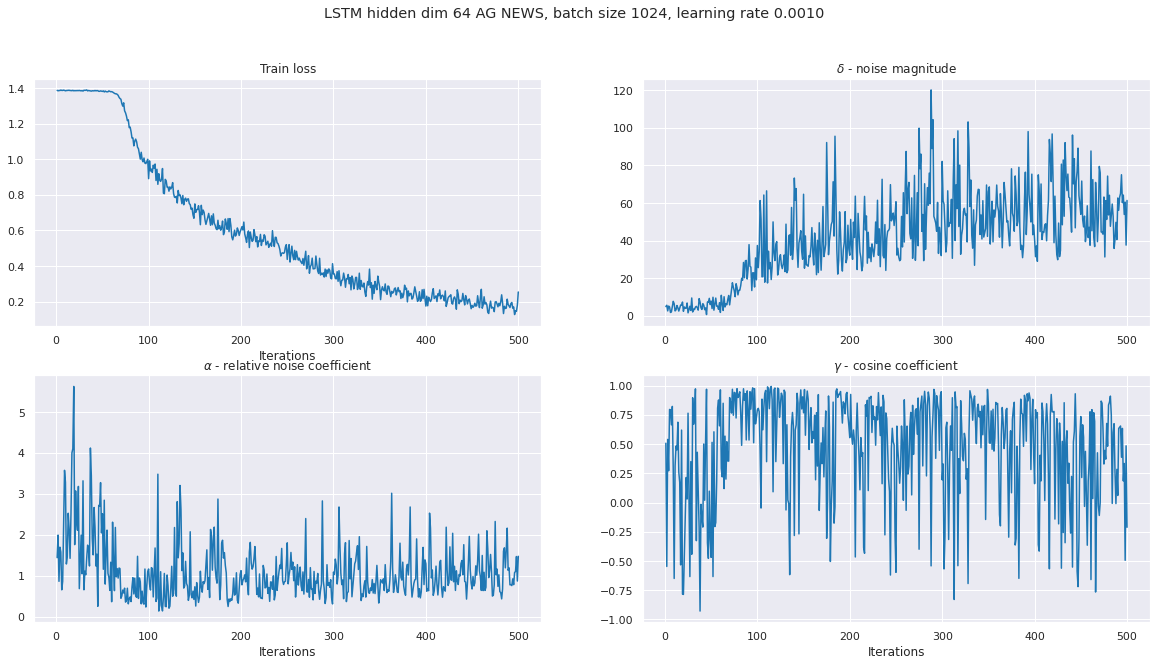
Figure 5: LSTM AG-News batch size - 1024

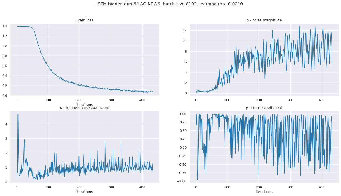
Figure 6: LSTM AG-News batch size - 8192

Then we investigate GRU [3] with 1 layer:

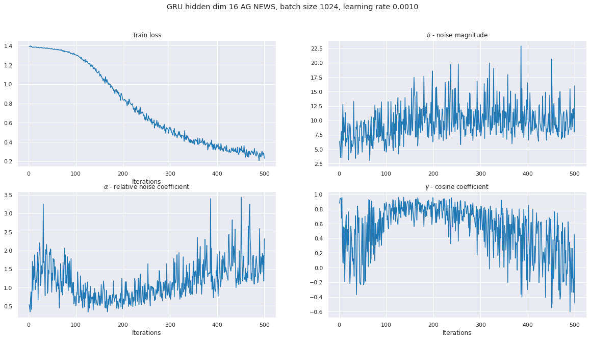
Figure 7: GRU AG-News batch size - 128

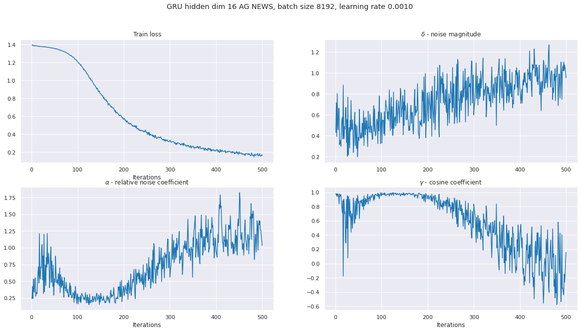
Figure 8: GRU AG-News batch size - 8192

8.3 Dataset consistency

We can reformulate condition 7.1 for arbitrary machine learning problem 4:

$$\begin{gathered}f(\theta)=\frac{1}{m}\sum_{k=1}^{m}f_{k}(\theta),\\ \langle\nabla{f_{k}}(\theta),\nabla{f_{j}}(\theta)\rangle\geqslant\Upsilon\|\nabla{f_{k}}(\theta)\|_{2}\|\nabla{f_{j}}(\theta)\|_{2}.\end{gathered}$$

Such condition may be motivated by consistency of dataset similarly to 18. Then we can guarantee $\langle\nabla{f}(\theta),\nabla f_{\xi}(\theta)\rangle\geqslant\Upsilon\|\nabla{f}(\theta)\|_{2}\|\nabla{f_{\xi}}(\theta)\|_{2}$. We calculate empirical distribution of cosine between two gradient samples on different epochs. We choose random 50 samples and calculate cosine if $i\not=j$.

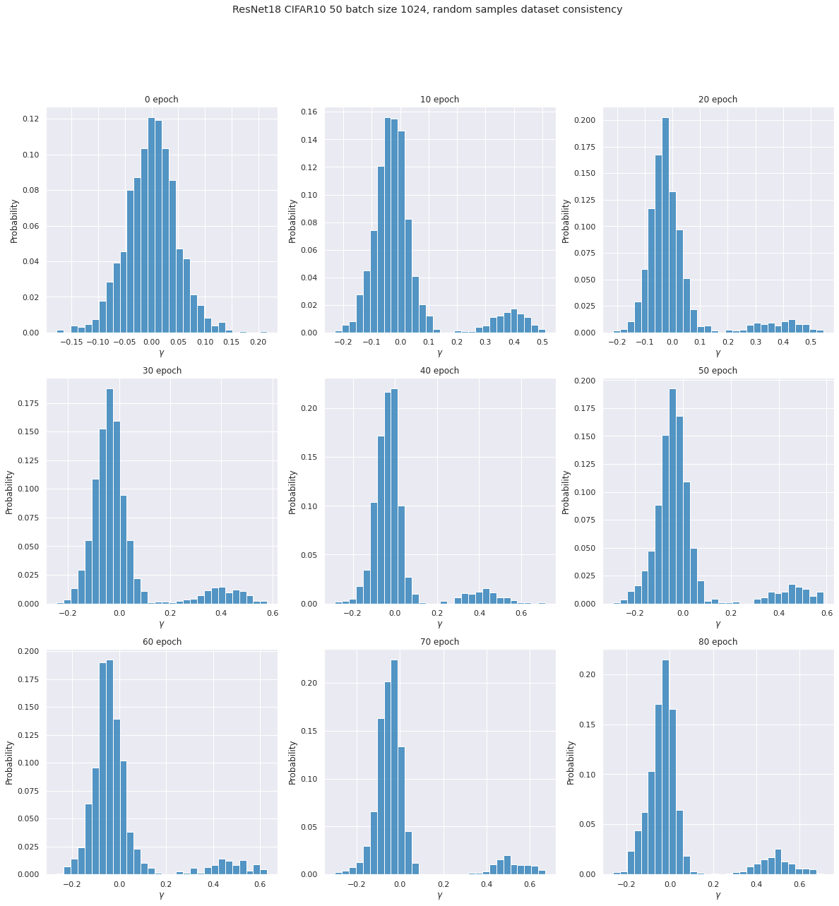
Figure 9: ResNet-18 CIFAR-10 dataset consistency

We can note, that empirical density can be described as mixture of two distributions. First is similar centered normal distribution, and the second one, which can corresponds to group of elements corresponds local convergence of method.

References

- [1] A. Beznosikov, A. Sadiev, and A. Gasnikov, Gradient-Free Methods with Inexact Oracle for Convex-Concave Stochastic Saddle-Point Problem, in International Conference on Mathematical Optimization Theory and Operations Research. Springer, 2020, pp. 105–119.
- [2] A. Beznosikov, S. Samsonov, M. Sheshukova, A. Gasnikov, A. Naumov, and E. Moulines, First order methods with markovian noise: from acceleration to variational inequalities, Advances in Neural Information Processing Systems 36 (2024).
- [3] J. Chung, C. Gulcehre, K. Cho, and Y. Bengio, Empirical evaluation of gated recurrent neural networks on sequence modeling, arXiv preprint arXiv:1412.3555 (2014).
- [4] O. Devolder, F. Glineur, and Y. Nesterov, First-order methods of smooth convex optimization with inexact oracle, Mathematical Programming 146 (2014), pp. 37–75.
- [5] P. Dvurechensky and A. Gasnikov, Stochastic intermediate gradient method for convex problems with stochastic inexact oracle, Journal of Optimization Theory and Applications 171 (2016), pp. 121–145. Available at http://dx.doi.org/10.1007/s10957-016-0999-6.
- [6] O. Gannot, A frequency-domain analysis of inexact gradient methods, Mathematical Programming 194 (2022), pp. 975–1016. Available at https://doi.org/10.1007/s10107-021-01665-8.
- [7] S. Guminov, A. Gasnikov, and I. Kuruzov, Accelerated methods for weakly-quasi-convex optimization problems, Computational Management Science 20 (2023), p. 36.
- [8] K. He, X. Zhang, S. Ren, and J. Sun, Deep residual learning for image recognition, in Proceedings of the IEEE conference on computer vision and pattern recognition. 2016, pp. 770–778.
- [9] D.P. Kingma and J. Ba, Adam: A method for stochastic optimization, arXiv preprint arXiv:1412.6980 (2014).
- [10] N. Kornilov, E. Gorbunov, M. Alkousa, F. Stonyakin, P. Dvurechensky, and A. Gasnikov, Intermediate gradient methods with relative inexactness, arXiv preprint arXiv:2310.00506 (2023).
- [11] A. Krizhevsky, G. Hinton, et al., Learning multiple layers of features from tiny images (2009).
- [12] A. Paszke, S. Gross, F. Massa, A. Lerer, J. Bradbury, G. Chanan, T. Killeen, Z. Lin, N. Gimelshein, L. Antiga, A. Desmaison, A. Kopf, E. Yang, Z. DeVito, M. Raison, A. Tejani, S. Chilamkurthy, B. Steiner, L. Fang, J. Bai, and S. Chintala, PyTorch: An Imperative Style, High-Performance Deep Learning Library, in Advances in Neural Information Processing Systems 32, H. Wallach, H. Larochelle, A. Beygelzimer, F. d’Alché Buc, E. Fox, and R. Garnett, eds. Curran Associates, Inc., 2019, pp. 8024–8035. Available at http://papers.neurips.cc/paper/9015-pytorch-an-imperative-style-high-performance-deep-learning-library.pdf.
- [13] H. Sak, A.W. Senior, and F. Beaufays, Long short-term memory recurrent neural network architectures for large scale acoustic modeling (2014).
- [14] A. Vasin, A. Gasnikov, P. Dvurechensky, and V. Spokoiny, Accelerated gradient methods with absolute and relative noise in the gradient, Optimization Methods and Software 38 (2023), pp. 1180–1229.
- [15] S. Vaswani, F. Bach, and M. Schmidt, Fast and faster convergence of sgd for over-parameterized models and an accelerated perceptron, in The 22nd International Conference on Artificial Intelligence and Statistics. PMLR, 2019, pp. 1195–1204.
- [16] B.E. Woodworth, K.K. Patel, and N. Srebro, Minibatch vs local sgd for heterogeneous distributed learning, Advances in Neural Information Processing Systems 33 (2020), pp. 6281–6292.
- [17] P. Xu, J. Chen, D. Zou, and Q. Gu, Global convergence of langevin dynamics based algorithms for nonconvex optimization, Advances in Neural Information Processing Systems 31 (2018).
- [18] X. Zhang, J. Zhao, and Y. LeCun, Character-level convolutional networks for text classification, Advances in neural information processing systems 28 (2015).