Nash equilibrium in a singular stochastic game between two renewable power producers with price impact

Abstract

In this paper we solve the general problem, already formulated in [2], of finding a Nash equilibrium between two agents who can install irreversibly photovoltaic panels in order to maximize their profits of selling the produced electricity net of installation costs, in the case that their cumulative installations have an impact on power prices. Starting from a static version of the game, we find out that there exists a region in the state space where Nash equilibrium dictates that both players install, and in some cases this optimal installation strategy is non-unique. We then come back to the original continuous time problem, which needs a generalization of the Verification Theorem present in [2], taking into account a lack of smoothness of the value functions and the possible non-uniqueness of optimal strategies seen above. Finally, we explicitly construct the equilibrium strategies and the value functions, which depend on the two free boundaries which separate the region where each player installs or waits.

Keywords: singular stochastic control, irreversible investment, variational inequality, singular stochastic games, Nash equilibria, market impact

MSC: 35C99; 35D99; 35K10; 49L12; 60G99; 60H30; 91B70; 93E20.

1 Introduction

The paper [9] formulates the problem of optimal irreversible installation of photovoltaic panels for a single power-producing company, willing to maximize the profits from selling electricity in the market on an infinite time horizon and under the constraint that the cumulative installation cannot exceed a given maximum capacity $\theta$, and assumed to be large enough that its installation has an impact on power price. More in detail, the power price is assumed to follow an Ornstein-Uhlenbeck (OU) process (which reflects the stylyzed fact, empirically observed in several markets, that power price could possibly be negative), where the long-term mean decreases linearly with respect to the cumulative installation. The resulting optimal control problem is of singular type, and the optimal strategy is to install the minimal capacity so that the power price is always lower than a given nonlinear function of the installed capacity, which is characterized by solving an ordinary differential equation deriving from a free-boundary problem.

The paper [2] is a first step in extending this problem to the case when $N$ companies are present in the market, and the price impact is due to the cumulative installations of all of them, now with the constraint that the sum of their total installations cannot exceed a given $\theta$. This problem can be formulated in several mathematical ways, among which the two most well-studied are that of Pareto optimum and Nash equilibrium. The problem of finding a Pareto optimum has been fully solved in [2]. However, the problem of finding a Nash equilibrium is much more technically demanding: [2] presents a verification theorem for the case $N=2$, which involves a system of variational inequalities, and fully solves only the case when no price impact is present. The aim of this paper is to solve the general case when price impact is present and a Nash equilibrium is reached by two players.

This problem is formulated as a nonzero-sum game of singular control, where the two players control one state variable each (their own cumulative installation) and these two state variables have a cumulative impact on a third one (the electricity price). The typical situation in these games, see e.g. [4, 5, 6, 7], is that the state space, where state variables can take values, is divided in a continuation region common to both players where they do not exercise control and let the system evolve, and two intervention regions, one for each player, where one player intervenes and the other one does not. However, this problem is more general, as the possibility that both players install simultaneously is explicitly present and must be taken into account: for this reason, we should introduce another region, where both players can install simultaneously.

In order to have an intuition of how this generalization should be implemented, we first present a static version of this game where the two players have both only one possibility of installing at the beginning of the game, when they can choose the amount of additional installed capacity, with the constraint that the sum of the resulting total capacities of both players cannot exceed $\theta$. This characterizes a 3-dimensional state space, which is the Cartesian product of the whole real line (where the power price $x$ lies) times the 2-dimensional simplex of size $\theta$ (where installed capacities $y=(y_{1},y_{2})$ lie). For a given initial level of power price $x$, the resulting Nash equilibrium can be explicitly characterized, and it requires to divide the 2-dimensional simplex in four regions, one being the no-installation region common to both players, two being the regions where only one of the players installs and the other one stays idle, and a fourth one being the region of joint installation. Depending on the price level $x$, some of these regions could be absent from the corresponding section of the state space, but in general one should take into account the presence of all four of them. While the players’ strategy in the first three regions is analogous to other examples in literature (i.e., each player either does not install, or installs enough power to arrive to the boundary of the common no-installation region), the novelty of this problem is the fourth region where both players install, which in this case is the intersection of a suitable square, depending on the price level $x$, with the simplex. In this region, both players install enough capacity to move their installation from their current state $y$ to the upper right corner of the square, net of the constraint $\theta$ on the capacity of the plant. Thus, if this vertex is inside the simplex, then they reach the same level of installed power; however if the vertex is outside of the simplex, then we have a non-uniqueness of Nash equilibria, as any admissible strategy which makes the two installations reach the simplex’s boundary is a Nash equilibrium.

Inspired by this, we pass to the continuous time formulation of our singular game. The first step is to review the verification theorem present in [2] by taking into account a possible non-uniqueness of strategies in the region of joint installation. In particular we select a preferred strategy at saturation by assuming that the players never install when their current level of installed power is greater or equal than $\frac{\theta}{2}$. As in [2], this results in two systems of variational inequalities, each one satisfied by the value function $V_{i}$ of player $i=1,2$. The first equation in the system $i$ is a variational inequality involving a second order operator in the space variable and a first order operator in $y_{i}$: it characterizes a continuation region $\mathbb{W}_{i}$ and an installation region $\mathbb{I}_{i}$, and has as domain the continuation region $\mathbb{W}_{j}$ of player $j\neq i$. The verification theorem in [2] also specifies a variational inequality on the domain $\mathbb{I}_{j}$, however we find out that it can be replaced by a much simpler first order equation on the variable $y_{j}$, thus simplifying the the task of constructing a solution. Moreover, we find out that there is also a loss of smoothness of the value functions from the case of optimal control to the case of games: in fact, we show that there may not exist a solution $V_{i}$ to the variational problem that is $C^{2}_{x}$ and $C^{1}_{y}$ on $\mathbb{W}_{j}$, as that would be not compatible, roughly speaking, with the optimality condition on $\mathbb{I}_{j}$. Therefore we generalize the verification theorem of [2] also in this direction, making use of a weak Itô formula, and allowing the solution to be not smooth on his own free boundary. This loss of smoothness is analogous to what happens e.g. when going from impulsive control to games, see [1] for this result and the relative discussion, or in optimal stopping problems, see [3] and the references therein.

Having established a verification theorem general enough, we are then able to build the solution of the problem, both in terms of solutions $V_{i}$, $i=1,2$ of the system of variational inequalities, as well as in terms of the corresponding free boundaries: since in this case the state space is three-dimensional, the resulting free boundaries are surfaces, in particular parameterized by $x=F_{i}(y)$, $i=1,2$. This allows to build the Nash equilibrium strategies in terms of reflected diffusions: these strategies are analogous to the one-player case of [9], i.e. they can possibly jump at the initial time and then they are continuous. More in detail, if the initial state $(x,y)\in\mathbb{I}_{i}\cap\mathbb{W}_{j}$, then only Player $i$ makes an instantaneous installation to hit the boundary of $\mathbb{I}_{i}$. Instead, if $(x,y)\in\mathbb{I}_{i}\cap\mathbb{I}_{j}$, then both players make an instantaneous installation to hit the separation boundary of the 4 regions: after this lump installation, the equilibrium strategy is to have always $Y^{1}_{t}=Y^{2}_{t}$ for all $t>0$. After this possible initial installation, the equilibrium strategy will always keep the process inside the closure of $\mathbb{W}_{1}\cap\mathbb{W}_{2}$. In particular, when $X_{t}$ hits the boundary of $\mathbb{I}_{i}$, then Player $i$ will install; this also includes the case when $X_{t}$ hits both the boundaries of $\mathbb{I}_{i}$ and $\mathbb{I}_{j}$ simultaneously: this will happen when $Y_{t}^{1}=Y_{t}^{2}$, in which case both players will install the same amount of capacity in order to keep this equality always satisfied.

The paper is organized as follows. In Section 2 we introduce the general problem of finding a Nash equilibrium between the two players, with all the relative definitions. In Section 3 we restrict the set of admissible strategies to those such that the two players can only perform one initial installation and then they cannot control the system anymore, and derive the relative Nash equilibria, with a possible non-uniqueness on the common installation region $\mathbb{I}_{1}\cap\mathbb{I}_{2}$. In Section 4 we come back to the general continuous-time game, presenting the relative Verification Theorem and the weak Ito formula used to prove it, and then constructing explicitly the equilibrium strategies.

2 A market with 2 players

Let $W$ be a standard one-dimensional Brownian motion on a complete filtered space $(\Omega,\mathcal{F},P,\{\mathcal{F}_{t}\}_{t\geq 0})$ and denote with $x$ a point in ${\mathbb{R}}$ and $y=(y_{1},y_{2})$ a point in ${\mathbb{R}}^{2}$. We assume that, in absence of any companies’ economic activities, the electricity price $(X^{x}_{t})_{t\geq 0}$ evolves according to a mean reverting Orstein-Uhlenbeck dynamics

$$dX^{x}_{t}=k\left(\mu-X^{x}_{t}\right)dt+\sigma dW_{t},\qquad X^{x}_{0}=x,$$

for some constants $k,\sigma$ and $\mu\in{\mathbb{R}}$.

We consider a market in which two producers, indexed by $i=1,2$, operate. The level of installed power of producer $i$ is described by the process

$$Y^{x,I,i}_{t}=y_{i}+I^{i}_{t},\qquad t\geq 0^{-},$$ (2.1)

where $y_{i}$ is the initial level of installed power, $I_{t}=(I_{t}^{1},I_{t}^{2})$ is the total power installed by the two producers within the interval $[0,t]$, and each component $I^{i}_{t}$ identifies the $i$ company’s control variable. We also assume that the total level of installed power cannot exceed a certain threshold $\theta$, since, for instance, only a finite real estate is available for the installation of solar panels or wind power plants. Accordingly, the set of admissible controls is given by

$${\mathcal{I}}(y)={\mathcal{I}}^{2,\theta}(y):=\{I:[0,\infty)\times\Omega\mapsto[0,\infty)^{2},\text{non-decreasing, cadlag},\;\sum_{i=1}^{2}(y_{i}+I^{i}_{t})\leq\theta\}.$$ (2.2)

Notice that each player is constrained, in its strategy, by the installation strategy of the other. Following [9] we assume that the current total level of electricity production, which is proportional to $\sum_{i=1}^{2}Y^{i}_{t}$, has a negative effect on the electricity price: its mean level at time $t$ is instantaneously reduced by a factor $\beta$ of $\sum_{i=1}^{2}Y^{i}_{t}$, for some $\beta>0$. Therefore, the spot price $(X^{x,y,I}_{t})_{t\geq 0}$ evolves according to

$$\begin{cases}dX^{x,y,I}_{t}=k\left(\mu-{\beta}\sum_{i=1,2}Y_{t}^{y,I,i}-X^{x,y,I}_{t}\right)dt+\sigma dW_{t},\qquad t>0,\\ X^{x,y,I}_{0}=x.\end{cases}$$ (2.3)

In this setting, each company aims at maximizing the profit, derived from selling electricity in the market, which for an admissible control $I$ is described by the following utility functional

$${\mathcal{S}}_{i}(x,y,I)=\mathbb{E}\left[\int_{0}^{\infty}e^{-\rho{\tau}}\,X^{x,y,I}_{\tau}\,Y^{y,I,i}_{\tau}\,d{\tau}-c\int_{0}^{\infty}e^{-\rho{\tau}}dI^{i}_{\tau}\right],$$ (2.4)

where $\rho$ is the discount factor and $c\geq 0$ is the constant representing the cost of installing one unit of power.

2.1 Problem formulation

In [2], the authors considered the cooperative situation of a social planner, where the problem consists of finding an efficient installation control $I\in{\mathcal{I}}^{2,\theta}(y)$ which maximizes the aggregate expected profit, net of investment cost. This is known as a Pareto optimum and is expressed as

$$\sup_{I\in{\mathcal{I}}^{2,\theta}(y)}{\mathcal{S}}_{SP}(x,y,I),\qquad{\mathcal{S}}_{SP}(x,y,I):={\mathcal{S}}_{1}(x,y,I)+{\mathcal{S}}_{2}(x,y,I).$$

Set $\bar{y}=y_{1}+y_{2}$ and $\bar{I}_{\tau}=I^{1}_{\tau}+I^{2}_{\tau}$, it is straightforward to check that

$${\mathcal{S}}_{SP}(x,y,I)=\bar{{\mathcal{S}}}_{SP}(x,\bar{y},\bar{I})=\mathbb{E}\left[\int_{0}^{\infty}e^{-\rho{\tau}}\,X^{x,y,I}_{\tau}\,(\bar{y}+\bar{I}_{\tau})\,d{\tau}-c\int_{0}^{\infty}e^{-\rho{\tau}}d\bar{I}_{\tau}\right].$$ (2.5)

Then the aggregate optimal strategy for the social planner is equivalent to the optimal control for a single player, as investigated in [9]. Such strategy does not characterize the single installations $I^{i}$, and it is indeed not unique. Notice as well that the problem can be formulated for $N$ players without any modification.

In this paper we look for an equilibrium solution to the competitive game between the two companies, also known as Nash equilibrium. Generally speaking, a Nash equilibrium is an optimal control for both players, in the sense that neither one can improve their profit by changing their control while the other keeps theirs unchanged. To precisely define the Nash equilibrium we will employ in our analysis, we first need to introduce some additional notations as well as the notion of admissible strategy.

Notation 2.1.

We denote by $D$ the two-dimensional simplex of size $\theta$, defined as

$$D:=\{y=(y_{1},y_{2})\in{\mathbb{R}}^{2},\;y_{i}\geq 0,\;y_{1}+y_{2}<\theta\},$$ (2.6)

which corresponds to the set of all possible installed power states. Moreover, for a given $t>0$, we denote by $C([0,t])$ and $\mathbb{D}([0,{t}];D)$ the sets of real-valued continuous functions and non-decreasing cadlag functions, respectively, defined on $[0,t]$.

Definition 2.2 (Admissible strategy).

A family ${\bf I}=({\bf I}_{t})_{t\geq 0}$ of Borel-measurable functions ${\bf I}_{t}:C([0,t])\times\mathbb{D}([0,{t}];D)\to{\mathbb{R}}^{2}$ such that, for any $(x,y)\in{\mathbb{R}}\times D$, there exists a unique $I\in\mathcal{I}(y)$ such that

$$I_{t}={\bf I}_{t}\big{(}(X^{x,y,I}_{s})_{s\leq t},(Y^{y,I}_{s-})_{s\leq t}\big{)},\qquad t\geq 0,$$ (2.7)

is called an admissible strategy. The set of all admissible strategies is denoted by $\mathcal{A}$.

Definition 2.3 (Nash equilibrium).

A function ${\bf I}\in\mathcal{A}$ is called a Nash equilibrium if, for any $\{i,j\}$ permutation of $\{1,2\}$ and $(x,y)\in{\mathbb{R}}\times D$ we have:

$${\mathcal{S}}_{i}(x,y,I)\geq{\mathcal{S}}_{i}(x,y,I^{\prime}),$$ (2.8)

with $I$ as in (2.7), for any $I^{\prime}\in\mathcal{I}(y)$ such that

$$I^{\prime j}_{t}={\bf I}^{j}_{t}\big{(}(X^{x,y,I^{\prime}}_{s})_{s\leq t},(Y^{y,I^{\prime}}_{s-})_{s\leq t}\big{)},\qquad t>0.$$ (2.9)

3 One step game

To develop an intuition on how a Nash equilibrium strategy should work and to introduce some key concepts for the subsequent analysis, we first look at the simpler case when both players can install only at time $t=0$. In this situation an admissible control (equivalently a strategy) for the player $i$ is completely determined by the deterministic value

$$I^{i}_{0}={\bf I}^{i}(x,y)\geq 0,\quad\text{s.t.}\quad\sum_{i=1}^{2}(y_{i}+I^{i}_{0})\leq\theta.$$

The expected profit can be computed exactly as

$$\mathcal{S}_{i}(x,y,I_{0})=(y_{i}+I^{i}_{0})\frac{x\rho+\mu k-\beta k\langle{\bf 1},y+I_{0}\rangle}{\rho(\rho+k)}-cI^{i}_{0},$$ (3.1)

which is a quadratic function of $I^{i}_{0}$. Then the equilibrium condition (2.8) of Definition 2.3 can be expressed as follows: the function ${\bf I}$ is a Nash equilibrium if, for any $\{i,j\}$ permutation of $\{1,2\}$ and $(x,y)\in{\mathbb{R}}\times D$, denoted $Y_{i}=y_{i}+I^{i}$, $Y^{\prime}_{i}=y_{i}+I^{\prime i}$, $i\in\{1,2\}$, we have

$$(Y^{\prime}_{i}-Y_{i})(2A(x)-Y_{j}-Y^{\prime}_{i}-Y_{i})\leq 0,\quad\forall\;Y^{\prime}_{i}\in[y_{i},\theta-Y_{j}],$$ (3.2)

where $A(x)$ is a linear function of the price at time $0$, precisely

$$A(x):=\frac{x\rho+\mu k-c\rho(\rho+k)}{2\beta k}.$$ (3.3)

3.1 Equilibrium strategies

For the rest of the Section we will denote $I=I_{0}$, $I^{\prime}=I^{\prime}_{0}$. Assume that the player $j$ chooses the optimal strategy $I^{j}$. Then we look for a strategy $I^{i}$ given by

$$I^{i}=\operatorname*{arg\,max}_{I^{\prime i}\in[0,\theta-y_{1}-Y_{2}]}\mathcal{S}_{i}(x,y,I^{\prime i},I^{j}).$$ (3.4)

Then, by a simple derivation of (3.1) it is easy to check that

$$I^{i}=\min\{\theta-Y_{j}-y_{i},+A(x)-\frac{1}{2}Y_{j}-y_{i}\}\vee 0.$$ (3.5)

This means that we can characterize $I^{i}$ by the geometric properties of the locus of points (3.5), depending on $A(x)$, i.e. a linear function of the price. Let us first consider the intersection of the lines

$$P(y)=\left\{(z_{1},z_{2})\in{\mathbb{R}}^{2},\;z_{i}=A(x)-\frac{1}{2}(y_{j}+z_{j})-y_{i},\{i,j\}=\{1,2\}\right\}=\left(\frac{2}{3}A(x)-y_{1},\frac{2}{3}A(x)-y_{2}\right),$$ (3.6)

which corresponds to the solution to the optimization problem in the absence of constrains. By (3.5) we can make the following preliminary observations:

• If $\frac{2}{3}A(x)-y_{i}\leq 0$, then $I^{i}=0$, $i=1,2$.

• If $\frac{2}{3}A(x)-y_{j}\leq 0$ and $\frac{2}{3}A(x)-y_{i}>0$, then by (3.5), $I^{i}=\min\{\theta-y_{1}-y_{2},A(x)-y_{i}-\frac{y_{j}}{2}\}\vee 0$. This means that, if $y\in D$, the player $i$ installs when $A(x)-y_{i}-\frac{y_{j}}{2}>0$ and saturates the capacity of the system if $A(x)+\frac{y_{j}}{2}\geq\theta$.

• If $\frac{2}{3}A(x)-y_{i}\geq 0$, $i=1,2$ then both players do install if $y\in D$.

Let us now visualize both players strategies, depending on the electricity price at time $0$. We may distinguish four cases:

• $A(x)\leq 0$: in this situation $\frac{2}{3}A(x)-y_{i}<0$, $i=1,2$ $\forall\,y\in\overline{D}$, therefore $I^{1}=I^{2}=0$. Roughly speaking, the electricity price is too low to justify any installation.

• $0\leq A(x)\leq\frac{\theta}{2}$: in this price interval one or both players may install, depending on the initial condition $y\in\overline{D}$. However the system will never reach saturation, since

  $$A(x)-\frac{1}{2}y_{i}<\theta-y_{i},\qquad y_{i}\in[0,\theta],\quad i=1,2.$$

  If $\frac{2}{3}A(x)-y_{i}>0$, $i=1,2$, i.e. the intersection point (3.6) corresponds to an admissible strategy, then

  $$I^{i}=\frac{2}{3}A(x)-y_{i},\qquad i=1,2.$$

  Notice that, regardless on the initial level of installed power, both players reach the same level after installation. We will comment again on this later.

  If $\frac{2}{3}A(x)-y_{i}\leq 0$ and $\frac{2}{3}A(x)-y_{j}>0$, by (3.5) we have $I^{i}=0$, and

  $$I^{j}=A(x)-\frac{1}{2}y_{i}-y_{j}\vee 0.$$ (3.7)

  Lastly, if $\frac{2}{3}A(x)-y_{i}\leq 0$, $i=1,2$, then $I^{1}=I^{2}=0$.

• $\frac{\theta}{2}<A(x)\leq\frac{3}{4}\theta$: this case is analogous to ii) until $\theta>y_{i}>2(\theta-A(x))\geq\frac{2}{3}A(x)$, $i=1,2$. On this subset we have indeed

  $$A(x)-\frac{1}{2}y_{i}>\theta-y_{i},$$

  and therefore the player $j$ must install up to saturating the capacity $\theta$. Precisely we have

  $$I_{i}=0,\qquad I_{j}=\theta-y_{i}-y_{j}.$$

  See Figure 1 for a visual representation of cases ii) and iii).

  

  

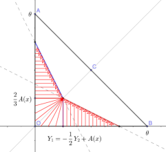
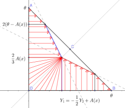
  Figure 1: Cases ii) and iii)

• $A(x)>\frac{3}{4}\theta$: in this price level, the system always reach a saturation state. Indeed, if $y_{i}<\frac{\theta}{2}$, then $A(x)-\frac{1}{2}y_{i}>\theta-y_{i}$, otherwise $A(x)-\frac{1}{2}y_{j}>\theta-y_{j}$, $\{i,j\}=\{1,2\}$.
  As before, if $y_{i}>\frac{2}{3}A(x)$, then $I_{i}=0$. Otherwise it is straightforward to check that the set

  $$I^{i}=\min\{\theta-y_{i}-y_{j}-I^{j},A(x)-\frac{1}{2}(y_{j}+I^{j})-y_{i}\},\quad\{i,j\}\in\{1,2\}$$

  corresponds to

  $$\left\{I^{i}+I^{j}=\theta-y_{i}-y_{j},\,I^{i}\geq 2(\theta-A(x))-y_{i},\;\{i,j\}=\{1,2\}\right\}.$$

  See for instance Figure 2.

  

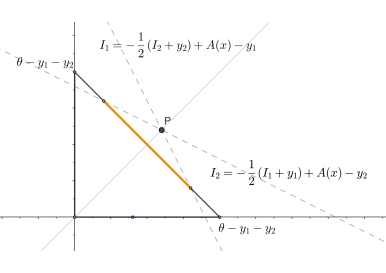
  Figure 2: Case iv), saturation at $y_{i}<\frac{2}{3}A(x)$

  This means that any admissible strategy which saturates the capacity of the system is an equilibrium strategy. In Figure 3 we show two possible strategies at saturation. The strategy a appears to be more regular with respect to $x$, while on the other hand, strategy b is easier to implement. Hereafter will set our analysis to match the latter idea.

  

  

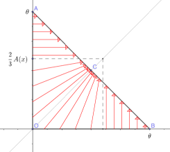
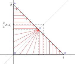
  Figure 3: Case iv), strategies a and b

The reader can easily check (3.2) through cases i) to iv).

3.2 The free boundary function

Let us examine figure 1 which corresponds to the cases (ii) and (iii) for reference. The set of points highlighted in blue can be interpreted as the level set of a boundary function $F_{1}:\overline{D}\mapsto{\mathbb{R}}$, separating what we might call the installation and waiting regions for the player 1. Similarly the points in red, with respect to a boundary function $F_{2}$. Clearly $F_{1}(y_{1},y_{2})=F_{2}(y_{2},y_{1})$ by the symmetry of the game.

In order to extend the computation above to the dynamic case, it is crucial to understand the structure of these regions and the free boundaries. For any $\{i,j\}\in\{1,2\}$ and $y\in\overline{D}\cap\{y_{i}\leq y_{j}\}$ we put

$$F_{i}(y)=A^{-1}\left(y_{i}+\frac{y_{j}}{2}\right).$$ (3.8)

Then we can characterize the waiting region for the player $i$ as follows:

$$\mathbb{W}^{i}:=W^{free}_{F_{i}}\cup W^{prol}_{F_{i}}\cup W^{sat}_{i},$$ (3.9)

with

$$W^{free}_{F_{i}} :=\left\{(x,y)\in{\mathbb{R}}\times\overline{D},\,y_{i}\leq y_{j},\,x<F_{i}(y)\right\},$$

$$W^{prol}_{F_{i}} :=\left\{(x,y)\in{\mathbb{R}}\times\overline{D},\,y_{i}>y_{j},y_{i}\leq\frac{\theta}{2}\,x<F_{i}(y_{i},y_{i})\right\},$$

$$W^{sat}_{i} :=\left\{(x,y)\in{\mathbb{R}}\times\overline{D},\,y_{i}>y_{j},y_{i}>\frac{\theta}{2}\right\}.$$

The component $W^{sat}_{i}$ matches the choice of strategy b in case iv): indeed player $i$ never installs if his current level of installed power is higher than $\frac{\theta}{2}$. On the other hand we put

$$\mathbb{I}^{i}:=({\mathbb{R}}\times\overline{D})\setminus\mathbb{W}^{i}.$$ (3.10)

In figure 4 we may observe the typical boundary structure on the three dimensional plane.

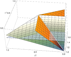
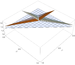
Figure 4: Boundary functions for $k=c=\rho=\mu=\theta=1$, $\beta=1/2$

Finally, let us characterize the strategy and value function with respect to the free boundary and the regions (3.9), (3.10). First, let

$$R_{i}(x,y):=S_{i}(x,y,0,0)=y_{i}\frac{x\rho+\mu k-{\beta}k\langle{\bf 1},y\rangle}{\rho(\rho+k)},\qquad(x,y)\in{\mathbb{R}}\times\overline{D},$$ (3.11)

be the expected profit associated to a non-installation strategy. Then it is clear that

$$S_{i}(x,y,I)=R_{i}(x,y+I).$$ (3.12)

Next, we set $F^{-1}:[F(0,0),\infty)\to[0,\theta/2]^{2}$ as

$$F^{-1}(x):=\begin{cases}\left(\frac{2}{3}A(x),\frac{2}{3}A(x)\right)&\quad\text{if}\quad x\in[F(0,0),F(\theta/2,\theta/2)],\\ \left(\frac{\theta}{2},\frac{\theta}{2}\right)&\quad\text{if}\quad x>F(\theta/2,\theta/2).\end{cases}$$ (3.13)

We also set $F_{1}^{-1}(\cdot,y_{2}):[F_{1}(0,y_{2}),\infty)\to[0,\theta-y_{2}]\times\{y_{2}\}$ as

$$F_{1}^{-1}(x,y_{2}):=\begin{cases}\left(A(x)-\frac{y_{2}}{2},y_{2}\right)&\quad\text{if}\quad x\in[F(0,y_{2}),F(\theta-y_{2},y_{2})],\\ (\theta-y_{2},y_{2})&\quad\text{if}\quad x>F(\theta-y_{2},y_{2}),\end{cases}$$ (3.14)

and accordingly, $F_{2}^{-1}(\cdot,y_{1}):[F_{1}(y_{1},0),\infty)\to\{y_{1}\}\times[0,\theta-y_{1}]$.

With these notations at hand we can characterize the equilibrium strategy as follows: if a player $i$ is in its installation region, and $j$ is not, then $i$ makes an installation $I^{i}=F^{-1}_{i}(x,y_{j})_{i}-y_{i}$, pushing the initial state of the system to the boundary of $\mathbb{W}^{i}$ (therefore $\mathbb{W}^{i}\cap\mathbb{W}^{j}$) in the direction $x,\,y_{j}$ constants. If $i$ and $j$ are both in their installation region, they both make an installation $I=F^{-1}(x)-y$, pushing the state on the boundary of $\mathbb{W}^{i}\cap\mathbb{W}^{j}$. Therefore, recalling (3.12) we have

$$V_{i}(x,y)=\begin{cases}R_{i}(x,y),&(x,y)\in\mathbb{W}^{i}\cap\mathbb{W}^{j}\\ R_{i}(x,F_{j}^{-1}(x,y_{i})),&(x,y)\in\mathbb{W}^{i}\cap\mathbb{I}^{j}\\ R_{i}(x,F_{i}^{-1}(x,y_{j}))-c(F_{i}^{-1}(x,y_{j})-y)_{i},&(x,y)\in\mathbb{I}^{i}\cap\mathbb{W}^{j}\\ R_{i}(x,F^{-1}(x))-c(F^{-1}(x)-y)_{i},&(x,y)\in\mathbb{I}^{i}\cap\mathbb{I}^{j}.\end{cases}$$ (3.15)

3.3 Comparison with Pareto optima

The Pareto optimum is an installation strategy which maximizes the aggregate expected profit

$$\sum_{i=1,2}\mathcal{S}_{i}(x,y_{1},y_{2},I_{1},I_{2}).$$

Again, this quantity can be computed exactly: denoting $\bar{y}=y_{1}+y_{2}$ and $\bar{I}=I_{1}+I_{2}$ we have

$$\sum_{i=1,2}\mathcal{S}_{i}(x,y_{1},y_{2},I_{1},I_{2}) =(\bar{y}+\bar{I})E\left[\int_{0}^{\infty}e^{-\rho\tau}S^{x,y,I}(\tau)d\tau\right]-c\bar{I}$$

$$=(\bar{y}+\bar{I})\frac{x\rho+\mu k-\beta k(\bar{y}+\bar{I})}{\rho(\rho+k)}-c\bar{I}$$

Optimizing w.r.t the cumulative installation $\bar{I}$ we get

$$\bar{I}=\min\{A(x)-\bar{y},\theta-\bar{y}\}\vee 0,$$ (3.16)

where $A(x)$ is as in (3.3). Clearly, depending on the proportion in which the two players install, there are infinite Pareto optima. However, even in the case $y_{1}=y_{2}$ and assuming $I_{1}=I_{2}$, the Pareto optimum is fundamentally different from the Nash equilibrium: for instance it is easy to see that for the former, the system reaches saturation for $A(x)\geq\theta$, while for the latter the system reach saturation earlier, when $A(x)\geq\frac{3}{4}\theta$.

   

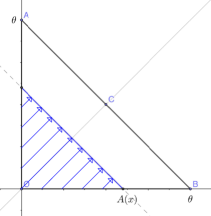
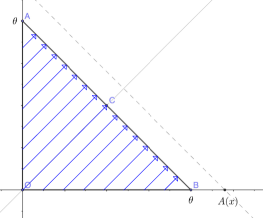
Figure 5: A possible Pareto optimum

3.4 Final remarks and ansatz for the general game

Similarly to the one step case, a Nash equilibrium for the general game will keep the state process $(X^{x,y,I}_{t},Y^{y,I}_{t})$ in the closure of $\mathbb{W}^{1}\cap\mathbb{W}^{2}$ by a possible lump installation at time $0$, and successive infinitesimal installations for $t>0$. With this in mind, the previous computations provide a good intuition on the structure of the regions $\mathbb{W}^{i}$ and $\mathbb{I}^{i}$, $i=1,2$. On one hand, the cross structure of the boundaries, as well as their monotonicity can be heuristically explained by the principle that the firm which has the least installed power should install before the other. Then, it would be also true that the joint installation region should be a square for every fixed $x$, as seen in Figures 1. Indeed, if that was not the case, then there would be states of the system which are transported to an installation region by any admissible control, see Figures 6 for reference.

   

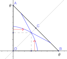
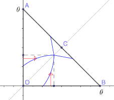
Figure 6: Two non-admissible boundaries

4 Continuous game

4.1 HJB free-boundary system and verification theorem

Let us now go back to the original problem. In this section we prove a verification theorem, which characterizes the equilibrium solution of the game.

First, let ${\mathcal{L}}$ denote the infinitesimal generator of the diffusion $(X_{t}^{x,y,0})_{t\geq 0}$, which is given by the second order operator

$${\mathcal{L}}f(x,y):=\frac{1}{2}{\partial}_{xx}f(x,y)+k(\mu-\beta y-x){\partial}_{x}f(x,y),$$ (4.1)

for $f(\cdot,y)\in C^{2}$, $y\subseteq O$ to be specified, and let $R_{i}(x,y)$ be the function defined in (3.11), which corresponds to the expected profit of firm $i$ when both firms follow a non-installation strategy. Finally, let $\{i,j\}$ be a permutation of $\{1,2\}$ and consider the variational PDE on the domain $D$:

$$\begin{cases}\max\{({\mathcal{L}}-\rho)V(x,y)+xy_{i},\,{\partial}_{y_{i}}V(x,y)-c\}=0,&\quad(x,y)\in\overline{W}\subset({\mathbb{R}}\times\overline{D})\\ {\partial}_{y_{j}}V(x,y)=0,&\quad(x,y)\in I=({\mathbb{R}}\times D)\setminus W\end{cases},$$ (4.2)

for an open set $W\subset{\mathbb{R}}\times{D}$, together with the boundary condition

$$V(x,y)=R_{i}(x,y),\qquad(x,y)\in\overline{AB}.$$ (4.3)

Definition 4.1 (Admissible boundary).

Let $\{i,j\}$ be a permutation of $\{1,2\}$. A real-valued function $F$ defined on $\overline{D}\cap\{y_{i}\geq y_{j}\}$ is called a $j$-admissible boundary if it is continuous and strictly increasing in both single variables.

Remark 4.2.

The restriction of an admissible boundary $F$ to the segment $\overline{OC}$ is monotonic increasing, i.e.

$$F(s,s)<F(r,r),\qquad 0\leq s<r\leq\theta/2.$$ (4.4)

Motivated by the analysis on the one-step problem, we define the waiting and installation regions of the players as follow:

Notation 4.3.

Let $\{i,j\}$ be a permutation of $\{1,2\}$. For any $j$-admissible boundary $F$, we set

$${\partial}F :=\{(x,y)\in{\mathbb{R}}\times D:y_{i}\geq y_{j},x=F(y)\},$$ (4.5)

which corresponds to the graph of the function F. Moreover we set

$$W^{\text{free}}_{F} :=\{(x,y)\in{\mathbb{R}}\times D:y_{i}\geq y_{j},x<F(y)\},$$ (4.6)

$$W^{\text{prol}}_{F} :=\{(x,y)\in{\mathbb{R}}\times D:y_{i}\leq y_{j},y_{j}<\theta/2,x<F(y_{j},y_{j})\},$$ (4.7)

$$W^{\text{sat}}_{F} :=\{(x,y)\in{\mathbb{R}}\times D:y_{j}\geq\theta/2\},$$ (4.8)

$$W_{F} :=W^{\text{free}}_{F}\cup W^{\text{prol}}_{F}\cup W^{\text{sat}}_{F},$$ (4.9)

$$I_{F} :=({\mathbb{R}}\times D)\setminus W_{F},$$ (4.10)

and $F^{-1}:[F(0,0),\infty)\to[0,\theta/2]$ as

$$F^{-1}(x):=\begin{cases}g^{-1}(x)&\quad\text{if}\quad x\in[F(0,0),F(\theta/2,\theta/2)],\\ \theta/2&\quad\text{if}\quad x>F(\theta/2,\theta/2),\end{cases}$$ (4.11)

where $g:=F|_{\overline{OC}}$.

We now introduce two reflection operators. Let ${\bf r}:{\mathbb{R}}^{2}\to{\mathbb{R}}^{2}$ given by

$${\bf r}(y_{1},y_{2})=(y_{2},y_{1}),$$ (4.12)

and its extension $\bar{\bf r}:{\mathbb{R}}\times{\mathbb{R}}^{2}\to{\mathbb{R}}\times{\mathbb{R}}^{2}$ given by

$$\bar{\bf r}(x,y)=\big{(}x,{\bf r}(y)\big{)}.$$ (4.13)

Let also the ${\mathcal{R}}:C(D)\to C(D)$ and $\bar{\mathcal{R}}:C({\mathbb{R}}\times D)\to C({\mathbb{R}}\times D)$ be acting, respectively, as

$${\mathcal{R}}(f)=f\circ{\bf r},\qquad\bar{\mathcal{R}}(f)=f\circ\bar{\bf r}.$$ (4.14)

Remark 4.4.

Let $\{i,j\}$ be a permutation of $\{1,2\}$. If $F$ is a $j$-admissible boundary, then ${\mathcal{R}}(F)$ is an $i$-admissible boundary and

$$W^{\text{free}}_{{\mathcal{R}}(F)}=\bar{\bf r}(W^{\text{free}}_{F}),\quad W^{\text{prol}}_{{\mathcal{R}}(F)}=\bar{\bf r}(W^{\text{prol}}_{F}),\quad W^{\text{sat}}_{{\mathcal{R}}(F)}=\bar{\bf r}(W^{\text{sat}}_{F}),\quad W_{{\mathcal{R}}(F)}=\bar{\bf r}(W_{F}),\quad I_{{\mathcal{R}}(F)}=\bar{\bf r}(I_{F}).$$ (4.15)

We now introduce a notion of solution that is useful to the resolution of the stochastic game. The idea is that the area $W_{F}$ is divided into a waiting region and an installation region, determined by a free-boundary function $G$.

Definition 4.5 (General solution to the variational PDE).

Let $\{i,j\}$ be a permutation of $\{1,2\}$ and $F$ be a $j$-admissible boundary. We say that a continuous function $V:{\mathbb{R}}\times\overline{D}\to{\mathbb{R}}$ is a (general) solution to the variational problem $\text{VP}_{\{i,j\}}(F)$ if

• ${\partial}_{y_{i}}V,\;{\partial}_{x}V\in C(\overline{W_{F}})$ and there exists a constant $L>0$ such that

  $${\left|({\partial}_{x}V)(x,y)-({\partial}_{x}V)(x^{\prime},y)\right|\leq L|x-x^{\prime}|,\qquad x,x^{\prime}\in{\mathbb{R}},\quad y\in\overline{D}.}$$ (4.16)

• the partial derivative ${\partial}_{y_{j}}V$ exists and is continuous on $I_{F}$ and a neighbourhood of ${\partial}F$. More precisely, there exists $r>0$ such that ${\partial}_{y_{j}}V\in C(U_{r})$, with $U_{r}:=(I_{F}+B_{r})\cap{D}$, where $B_{r}$ denotes the Euclidean ball centred at the origin, with radius $r$;

• there exists $K>0$ such that

  $$|V(x,y)|\leq K(1+|x|),\qquad(x,y)\in{\mathbb{R}}\times\overline{D};$$ (4.17)

and if (4.2)-(4.3) is satisfied weakly in $x$ on ${\mathbb{R}}\times D$, with $W=W_{F}$.

We now introduce the notion of regular solution, which is useful to the resolution of the stochastic game. The idea is that the area $W_{F}$ is divided into a waiting region and an installation region, determined by a free-boundary function $G$.

Definition 4.6 (Regular solution to the variational PDE).

Let $\{i,j\}$ be a permutation of $\{1,2\}$ and $F$ be a $j$-admissible boundary. We say that a pair $(V,G)$ is a regular solution to the variational problem $\text{VP}_{\{i,j\}}(F)$ if

• $V$ is a general solution to the variational problem $\text{VP}_{\{i,j\}}(F)$

• $G$ is an $i$-admissible boundary

• ${\partial}_{xx}V\in C(W_{F}\setminus{\partial}G)$, and it holds that

  $$({\mathcal{L}}-\rho)V(x,y)+xy_{1}=0,\ {\partial}_{y_{i}}V(x,y)-c\leq 0, \qquad(x,y)\in{W^{G}_{F}},$$ (4.18)

  $$({\mathcal{L}}-\rho)V(x,y)+xy_{1}\leq 0,\ {\partial}_{y_{i}}V(x,y)-c=0, \qquad(x,y)\in I^{G}_{F},$$ (4.19)

  where

  $${W^{G}_{F}:=W_{F}\cap W_{G}},\qquad I^{G}_{F}:=W_{F}\setminus\overline{W^{G}_{F}}.$$ (4.20)

Such $G$ is called a free-boundary function for $\text{VP}_{\{i,j\}}(F)$.

Remark 4.7.

At this stage, the regularity requirements on $V$ may seem convoluted at first sight. For instance, on the waiting region $W_{F}$ (of player $j$), one would expect to find second order regularity on the spatial variable, in order for the variational equation to be well defined everywhere as in the single player control setting [9]. However, it is common to observe a loss in regularity when passing from a control setting to the associated games, see discussion in [1], in the context of impulsive games. Similarly, in optimal stopping times it is generally difficult to prove that the value is regular up to the free boundary, see the discussion and examples in [3].

Our requirement are chosen to be somehow the minimal natural ones on $V$ in order to prove a verification theorem. In Section 4.3.2 we will further discuss these regularity aspects in the context of the construction of the free boundaries, and importantly, we will show that requiring the second order regularity on $W_{F}$ would actually prevent us from finding an equilibrium solution. On the other hand we still expect to obtain at least the Lipschitz continuity of the gradient in $x$, which, together with the monotonicity of the boundary $F$, allow us to employ an Itô formula which does not involve local times. As for the regularity in $y_{j}$, we require that the second equation in (4.2) is well defined slightly beyond his natural domain $I_{F}$.

We are now in the position to state the HJB-system associated to the Nash equilibria of our stochastic game.

Definition 4.8 (Equilibrium solution to the variational PDE).

We say that a pair $(V,F)$ is an equilibrium solution to VP if $F$ is a $2$-admissible boundary and $(V,{\mathcal{R}}(F))$ is a regular solution to the variational problem $\text{VP}_{\{1,2\}}(F)$.

Remark 4.9 (Symmetry).

It is straightforward to see that $(V,F)$ is an equilibrium solution to VP if and only if ${\mathcal{R}}(F)$ is a $1$-admissible boundary and $(\bar{\mathcal{R}}(V),F)$ is a regular solution to the variational problem $\text{VP}_{\{2,1\}}(F)$.

Notation 4.10.

If $(V,F)$ is a fixed equilibrium solution to VP, we set

$$F_{2}:=F,\quad V_{1}:=V, F_{1}:={\mathcal{R}}(F),\quad V_{2}:=\bar{\mathcal{R}}(V)$$ (4.21)

$$\mathbb{W}^{2}:=W_{F_{2}},\quad\mathbb{I}^{2}:=I_{F_{2}}, \mathbb{W}^{1}:=W_{F_{1}},\quad\mathbb{I}^{1}:=I_{F_{1}}.$$ (4.22)

Definition 4.11 ($j$-optimal strategy).

Let $j\in\{1,2\}$, $F$ a $j$-admissible boundary and $(x,y)\in{\mathbb{R}}\times{D}$. A control $I\in{\mathcal{I}}(y)$ is called $j$-optimal with respect to $F$ and $(x,y)$ if both the following conditions hold $\mathbb{P}$-almost surely:

$$(X^{x,y,I}_{t},Y^{y,I}_{t})\in\overline{W_{F}}{\cup(\,\overline{AB}\times{\mathbb{R}})}, t>0,$$ (4.23)

$$(X^{x,y,I}_{t},Y^{y,I}_{t})\in W_{F}\Rightarrow{dY^{y,I,j}_{t+}}=0, t>0,$$ (4.24)

and if $I^{j}$ is continuous with

$$I^{j}_{0}=\min\{s\geq 0:(x,y+s\,e_{j})\in\overline{W_{F}}\}.$$ (4.25)

Theorem 4.12 (Verification theorem).

Let $(V,F)$ be an equilibrium solution to VP. Let also ${\bf I}^{\star}\in\mathcal{A}$ such that, for any $j=1,2$ and $(\bar{x},\bar{y})\in{\mathbb{R}}\times{D}$, every control process $I\in\mathcal{I}(y)$ such that

$$I^{j}_{t}:={\bf I}_{t}^{\star,j}\big{(}(X^{\bar{x},\bar{y},I}_{s})_{s\leq t},(Y^{\bar{y},I}_{s-})_{s\leq t}\big{)},\qquad t\geq 0,$$ (4.26)

is $j$-optimal w.r.t. $F_{j}$ and $(\bar{x},\bar{y})$.

Then ${\bf I}^{\star}$ is a Nash equilibrium and

$${\mathcal{S}}_{i}(\bar{x},\bar{y};I^{\star})=V_{i}(\bar{x},\bar{y}),\qquad(\bar{x},\bar{y})\in{\mathbb{R}}\times D,\quad i=1,2,$$ (4.27)

where $I^{\star}\in\mathcal{I}(\bar{y})$ is the unique admissible control such that

$$I^{\star}_{t}={\bf I}_{t}^{\star}\big{(}(X^{\bar{x},\bar{y},I^{\star}}_{s})_{s\leq t},(Y^{\bar{y},I^{\star}}_{s-})_{s\leq t}\big{)},\qquad t\geq 0,$$ (4.28)

in accordance with Definition 2.2.

To prove Theorem 4.12 we need some preliminary results. Lemma 4.13 below guarantees that the value function is smooth outside a set of probability zero. This would be clear if the law of $(X^{x,y,I},Y^{y,I})$ were absolutely continuous with respect to the Lebesgue measure, however the marginal law of $Y^{y,I}$ is not, a priori, absolutely continuous, and no information is available for the joint law of the process. We we do exploit is the monotonicity of $F,Y^{y,I}$ and the fact that $I$ is optimal with respect of F. This allows us to prove an ad hoc Itô formula, accounting for the lack of regularity in the proof of the verification theorem.

Lemma 4.13.

Let $\{i,j\}$ be a permutation of $\{1,2\}$, let $G$, $F$ be an $i$-admissible boundary and a $j$-admissible boundary respectively, and $(x,y)\in{\mathbb{R}}\times{D}$. If $I\in{\mathcal{I}}(y)$ is $j$-optimal with respect to $F$ and $(x,y)$, we have

$${P\left((X^{x,y,I}_{t},Y^{y,I}_{t})\in{\partial}F\cup{\partial}G\right)=0,\qquad a.e.\quad t\geq 0.}$$ (4.29)

Proof.

We first prove the statement in the control setting of [9]. Assume for the moment that there is one player involved in the game with an initial installed capacity $y<\theta$. Assume $F:[0,\theta]\mapsto{\mathbb{R}}$ is a continuous and strictly increasing function and

$${\bf F}^{-1}(x)=\begin{cases}0,&x<F(0),\\ F^{-1}(x),&x\in{[F(0),F(\theta))},\\ \theta,&{x\geq F(\theta)}.\end{cases}.$$

Assume that the installed capacity evolves according to

$$Y^{y,I^{\star}}_{t}=y+I^{\star}_{t},\qquad I^{\star}_{t}={\bf I}^{\star}_{t}\big{(}(X^{x,y,I^{\star}}_{s})_{s\leq t},(Y^{y,I^{\star}}_{s})_{s\leq t}\big{)},$$ (4.30)

where

$${\bf I}^{\star}_{t}\big{(}({\bf x}_{s})_{s\leq t},({\bf y}_{s})_{s\leq t}\big{)}:=\Big{(}\sup_{s\leq t}{\bf F}^{-1}({\bf x}_{s})-{\bf y}_{0-}\Big{)}^{+},\qquad t\geq 0,\ {\bf x}\in C([0,t]),\ {\bf y}\in\mathbb{D}([0,{t}];[0,\theta[).$$ (4.31)

In particular, the strategy $I^{\star}$ is optimal with respect to $F$, in the sense that $X_{t}^{x,y,I^{\star}}\leq F(Y_{t}^{y,I^{\star}})$ for all $t>0$ and $dY^{y,I^{\star}}_{t*}=0$ if $X_{t}^{x,y,I^{\star}}<F(Y_{t}^{y,I^{\star}})$ by construction. When $F$ is the free boundary, it corresponds to the optimal control in [9]. Observe now that $Y_{t}^{y,I^{\star}}$ is bounded. Thus, by Girsanov’s theorem (see [10], Theorem 10.5), there exists an equivalent measure $\widetilde{\mathbb{P}}$ and a Brownian motion $\widetilde{W}_{t}$, such that the dynamics of $X^{x,y,I^{\star}}$ is

$$dX^{x}_{t}=k\left(\mu-X^{x}_{t}\right)dt+\sigma d\widetilde{W}_{t},\qquad X^{x}_{0}=x.$$ (4.32)

Consider the event

$$A_{t}:=\{(X^{x}_{t},Y^{y,I^{\star}}_{t})\in\partial F\}=\{X_{t}^{x}=F(Y^{y,I^{\star}}_{t})\}.$$ (4.33)

Then by (4.31) and monotonicity we have

$$\widetilde{\mathbb{P}}(A_{t}) =\widetilde{\mathbb{P}}\Big{(}X_{t}^{x}=F\Big{(}\sup_{s\leq t}{\bf F}^{-1}(X^{x}_{s})\Big{)}\Big{)}=\widetilde{\mathbb{P}}\Big{(}X_{t}^{x}=F\Big{(}{\bf F}^{-1}\Big{(}\sup_{s\leq t}X^{x}_{s}\Big{)}\Big{)}\Big{)}$$

$$=\underbrace{\widetilde{\mathbb{P}}\Big{(}(X_{t}^{x}=F(0))\cap\Big{(}\sup_{s\leq t}X^{x}_{s}<F(0)\Big{)}\Big{)}+\widetilde{\mathbb{P}}\Big{(}(X_{t}^{x}=F(\theta))\cap\Big{(}\sup_{s\leq t}X^{x}_{s}{\geq}F(\theta)\Big{)}\Big{)}}_{=0}$$

$$\qquad+\widetilde{\mathbb{P}}\Big{(}\Big{(}X_{t}^{x}=\sup_{s\leq t}X^{x}_{s}\Big{)}\cap\Big{(}\sup_{s\leq t}X^{x}_{s}\in[F(0),F(\theta))\Big{)}\Big{)}$$

$$\leq\widetilde{\mathbb{P}}\Big{(}X_{t}^{x}=\sup_{s\leq t}X^{x}_{s}\Big{)}=0,$$

where the last equality stems from the fact that the random time $\operatorname*{arg\,max}_{s\leq t}X^{x}_{s}$ has an absolutely continuous distribution on $[0,t]$. This is a well known fact when $X$ is a Brownian motion (see, for instance [8], Chapter 2.8), then it holds for the O-U process (4.32) by a second change of measure. In particular, this show that in the control setting of [9], if $F$ is the free boundary and the player acts optimally, then (4.29) holds true. Also note that $I^{\star}$ is the optimal strategy w.r.t $F$ which keeps the state $(X^{x}_{t},Y^{y,I}_{t})$ closer to the boundary.

Let’s now go back to the two players setting and fix $j=2$ w.l.o.g. Consider

$$B_{t}=\big{\{}(X^{x,y,I}_{t},Y^{y,I}_{t})\in{\partial}F\big{\}}=\Big{\{}\big{(}F(Y^{y,I}_{t})=X^{x,y,I}_{t}\big{)}\cap\sum_{i=1}^{2}Y^{y,I,1}_{t}<\theta\Big{\}}.$$

Clearly $B_{t}\subseteq\{Y^{y,I,2}_{t}\leq Y^{y,I,1}_{t}\}\cap\big{\{}(X^{x,y,I}_{t},Y^{y,I}_{t})\in\overline{W_{F_{1}}}\big{\}}$. Since $I$ is 2-optimal we have $F(Y^{y,I}_{s})\geq X^{x,y,I}_{s}$ $\forall\;s\in{\mathbb{R}}_{+}$, then by monotonicity $F(Y^{y,I}_{\tau})\geq X^{x,y,I}_{s}$ $\forall\;s\in[0,\tau]$. Thus we have

$$Y^{y,I,2}_{\tau}\geq(F(Y^{y,I,1}_{\tau},\cdot))^{-1}(X^{x,y,I}_{s}),\quad\forall\;s\in[0,\tau].$$

Finally, we infer

$$\mathbb{P}\big{(}B_{t}\big{)}\leq\mathbb{P}\Big{(}X^{x,y,I}_{t}=F\big{(}Y^{y,I,1}_{t},\sup_{s\leq t}(F(Y^{y,I,1}_{t},\cdot))^{-1}(X^{x,y,I}_{s})\big{)}\Big{)}=\mathbb{P}\big{(}X^{x,y,I}_{t}=\sup_{s\leq t}X^{x,y,I}_{s}\big{)},$$ (4.34)

again by monotonicity. The RHS of (4.34) can be treated as in the one player case by means of a Girsanov change of probability, yielding $\mathbb{P}(B_{t})=0$. Finally, the case $(X^{x,y,I}_{t},Y^{y,I}_{t})\in{\partial}G$ can be treated by comparison principle, using again the monotonicity of $I_{1}$. ∎

Lemma 4.14 (Itô formula).

Let $\{i,j\}$ be a permutation of $\{1,2\}$, and let $G$, $F$ be an $i$-admissible boundary and a $j$-admissible boundary respectively. Let $V:{\mathbb{R}}\times D\to{\mathbb{R}}$ such that conditions (i)-(ii) of Definition 4.5 hold true, and such that ${\partial}_{xx}V\in C(W_{F}\setminus{\partial}G)$. Then, for any $(\bar{x},\bar{y})\in{\mathbb{R}}\times{D}$, and any $I\in{\mathcal{I}}(\bar{y})$ $j$-optimal with respect to $F$ and $(\bar{x},\bar{y})$, we have

$$V(X^{\bar{x},\bar{y},I}_{t},Y^{\bar{y},I}_{t}) =V({\bar{x},\bar{y}})+\int_{0}^{t}{\mathcal{L}}V(X^{\bar{x},\bar{y},I}_{s},Y^{\bar{y},I}_{s})ds+\sigma\int_{0}^{t}\partial_{x}V(X^{\bar{x},\bar{y},I}_{s},Y^{\bar{y},I}_{s})\,dW_{s}$$ (4.35)

$$\quad+\int_{0}^{t}\big{\langle}\nabla_{y}V(X^{\bar{x},\bar{y},I}_{s},Y^{\bar{y},I}_{s}),dI^{c}_{s}\big{\rangle}+\sum_{{0\leq s\leq t}}\big{(}V(X^{\bar{x},\bar{y},I}_{s},Y^{\bar{y},I}_{s})-V(X^{\bar{x},\bar{y},I}_{s},Y^{\bar{y},I}_{s-})\big{)},\qquad t\geq 0.$$ (4.36)

Remark 4.15.

Note that the regularity conditions (i)-(iii) in Definition 4.6 are sufficient to write (4.35). The j-optimality of $I$ guarantees that the process $(X^{\bar{x},\bar{y},I}_{t},Y^{\bar{y},I}_{t})\in\overline{W}_{F}$ for any $t>0$ so that the partial derivative ${\partial}_{y_{i}}V$ appearing in (4.35) is well defined. Moreover, when $(X^{\bar{x},\bar{y},I}_{t},Y^{\bar{y},I}_{t})\in W_{F}\cup\overline{W^{\text{sat}}_{F}}$, then $dY^{x,I,j}=0$ by (4.24), so that ${\partial}_{y_{j}}V$ only need to be well defined in a neighbourhood of ${\partial}F$. In particular, by the monotonicity of $I$, once the process $(X_{t}^{x,y,I},Y_{t}^{y,I,j})$ enters the set $\overline{W_{F}^{\text{sat}}}$ it will never leave. Finally, the second order derivative ${\partial}_{xx}V$ is intended as a weak derivative.

Proof.

Let us fix $(\bar{x},\bar{y})\in\overline{W_{F}}$, and $I\in{\mathcal{I}}(y)$ $j$-optimal with respect to $F$ and $(\bar{x},\bar{y})$. To ease notation, we will drop the superscripts in the processes $X^{\bar{x},\bar{y},I}$ and $Y^{\bar{y},I}$, and fix $\{i,j\}=\{1,2\}$ throughout the proof. Note that, it is not restrictive to assume $(\bar{x},\bar{y})\in\overline{W_{F}}$. Indeed, if $(\bar{x},\bar{y})\in\overline{I_{F}}$, we have

$$V(X_{t},Y_{t})-V(\bar{x},\bar{y})=V(X_{t},Y_{t})-V(X_{0},Y_{0})+V(X_{0},Y_{0})-V(\bar{x},\bar{y}),$$ (4.37)

where $(X_{0},Y_{0})=(\bar{x},\bar{y}+I_{0})\in\overline{W_{F}}$ by Definition 4.11. For simplicity, we also assume $\bar{y}_{2}<\theta/2$. The proof of the case $\bar{y}_{2}\geq\theta/2$ is a simpler modification as $Y_{t}^{y,I,2}=\bar{y}_{2}$ for any $t>0$ (see Remark 4.15).

Note that (4.24) implies

$$(X_{t},Y_{t})\in\overline{W_{F}\setminus W_{F}^{\text{sat}}},\qquad t>0.$$ (4.38)

In particular, we have

$$Y^{2}_{t}=\theta/2,\qquad t\geq\tau_{2,\text{sat}},$$ (4.39)

where $\tau_{2,\text{sat}}$ is the stopping time

$$\tau_{2,\text{sat}}:=\begin{cases}\inf J_{2,\text{sat}}&\text{if }J_{2,\text{sat}}\neq\emptyset\\ +\infty&\text{otherwise}\end{cases},\qquad J_{2,\text{sat}}:=\{t>0:Y^{2}_{t}=\theta/2\}.$$ (4.40)

We also have

$$Y_{t}=Y_{\tau_{\text{sat}}},\qquad t\geq\tau_{\text{sat}},$$ (4.41)

where $\tau_{\text{sat}}$ is the stopping time

$$\tau_{\text{sat}}:=\begin{cases}\inf J_{\text{sat}}&\text{if }J_{\text{sat}}\neq\emptyset\\ +\infty&\text{otherwise}\end{cases},\qquad J_{\text{sat}}:=\{t>0:Y^{1}_{t}+Y^{2}_{t}=\theta\}.$$ (4.42)

Note that $\tau_{2,\text{sat}}\leq\tau_{\text{sat}}$.

We first set a regularizing in $x$ sequence $V^{n}$, obtained by convolution with the standard mollifiers: more precisely

$${{V}^{n}(x,y)=(V(\cdot,y)\star n\phi(n\cdot))(x),\qquad(x,y)\in D.}$$ (4.43)

where $\phi\in C^{\infty}_{0}$ is such that $supp(\phi)\subseteq B_{1}$ and has unity integral. Next we regularize w.r.t $y$: for ${\varepsilon}>0$ we take

$${{V}^{n,{\varepsilon}}(x,y)=\frac{1}{{\varepsilon}^{2}}\int_{y_{1}}^{y_{1}+{\varepsilon}}\int_{y_{2}}^{y_{2}+{\varepsilon}}{V^{n}}(x,z)dz_{1}dz_{2},\quad(x,y)\in{\mathbb{R}}\times D.}$$ (4.44)

Then ${\partial}_{x}V^{n,{\varepsilon}}(x,y)$, ${\partial}_{xx}{V}^{n,{\varepsilon}}(x,y)$ and $\nabla_{y}{V}^{n,{\varepsilon}}(x,y)$ are continuous and the derivatives read

$${\partial}^{k}_{x}{V}^{n,{\varepsilon}}(x,y) =\frac{1}{{\varepsilon}^{2}}\int_{y_{1}}^{y_{1}+{\varepsilon}}\int_{y_{2}}^{y_{2}+{\varepsilon}}{\partial}^{k}_{x}{V^{n}}(x,z)dz_{1}dz_{2},\qquad k=1,2,$$ (4.45)

$${\partial}_{y_{1}}{V}^{n,{\varepsilon}}(x,y) =\frac{1}{{\varepsilon}^{2}}\int_{y_{2}}^{y_{2}+{\varepsilon}}\left({V}^{n}(x,y_{1}+{\varepsilon},z_{2})-{V}^{n}(x,y_{1},z_{2})\right)dz_{2},$$ (4.46)

$${\partial}_{y_{2}}{V}^{n,{\varepsilon}}(x,y) =\frac{1}{{\varepsilon}^{2}}\int_{y_{1}}^{y_{1}+{\varepsilon}}\left({V}^{n}(x,z_{1},y_{2}+{\varepsilon})-{V}^{n}(x,z_{1},y_{2})\right)dz_{1}.$$ (4.47)

By (4.45) we directly infer that, for any compact set $K\subset{\mathbb{R}}^{3}$

$${\partial}^{k}_{x}{V}^{n,{\varepsilon}}(x,y)\overset{{\varepsilon}\to 0}{\rightrightarrows}{\partial}^{k}_{x}{V}^{n}(x,y),\qquad(x,y)\in{\overline{W_{F}}}\cap K,\quad k=0,1,2.$$ (4.48)

Moreover, for any $(x,y)\in{\overline{W_{F}}}$

$$\left|{\partial}_{y_{1}}{V}^{n,{\varepsilon}}(x,y)-{\partial}_{y_{1}}{V}^{n}(x,y)\right| \leq\frac{1}{{\varepsilon}}\int_{y_{2}}^{y_{2}+{\varepsilon}}\left|\frac{{V}^{n}(x,y_{1}+{\varepsilon},z_{2})-{V}^{n}(x,y_{1},z_{2})}{{\varepsilon}}-{\partial}_{y_{1}}{V}^{n}(x,y_{1},z_{2})\right|dz_{2}$$

$$=\int_{0}^{1}\left|\frac{{V}^{n}(x,y_{1}+{\varepsilon},y_{2}+{\varepsilon}\lambda)-{V}^{n}(x,y_{1},y_{2}+{\varepsilon}\lambda)}{{\varepsilon}}-{\partial}_{y_{1}}{V}^{n}(x,y_{1},y_{2}+{\varepsilon}\lambda)\right|d\lambda=o({1}).$$

The crucial point here is the fact that $(x,y_{1}+{\varepsilon},y_{2}+{\varepsilon}\lambda)$ and $(x,y_{1},y_{2}+{\varepsilon}\lambda)\in W_{F}$ for any ${\varepsilon},\,\lambda>0$ since $F$ is increasing in both variables. This observation then allows us to exploit conditions (i)-(iii) of Definition 4.5 for ${\varepsilon}$ small enough. Therefore it also holds that

$${\partial}_{y_{1}}{V}^{n,{\varepsilon}}(x,y)\overset{{\varepsilon}\to 0}{\rightrightarrows}{\partial}_{y_{1}}{V}^{n}(x,y),\qquad(x,y)\in{\overline{W_{F}}}\cap K.$$ (4.49)

Analogously, by the monotonicity of $F$ we can show that

$${\partial}_{y_{2}}{V}^{n,{\varepsilon}}(x,y)\overset{{\varepsilon}\to 0}{\rightrightarrows}{\partial}_{y_{2}}{V}^{n}(x,y),\qquad(x,y)\in(U_{r}\cap{\overline{W_{F}}})\cap K.$$ (4.50)

Next we apply the standard Itô formula to ${V}_{n,{\varepsilon}}$. For any $R>0$ set

$$\tau_{R}:=\begin{cases}\inf J_{R}&\text{if }J_{R}\neq\emptyset\\ R&\text{otherwise}\end{cases},\qquad J_{R}:=\{t>0:X^{\bar{x},\bar{y},I}_{t}\not\in(-R,R)\}.$$ (4.51)

Then we have

$${{V}^{n,{\varepsilon}}(X_{t\wedge\tau_{R}},Y_{t\wedge\tau_{R}})} ={V}^{n,{\varepsilon}}(\bar{x},\bar{y})+\int_{0}^{t\wedge\tau_{R}}{\mathcal{L}}{V}^{n,{\varepsilon}}(X_{s},Y_{s})ds+\sigma\int_{0}^{t\wedge\tau_{R}}\partial_{x}{V}^{n,{\varepsilon}}(X_{s},Y_{s})\,dW_{s}$$ (4.52)

$$\quad+{\int_{0}^{t\wedge\tau_{R}\wedge\tau_{2,\text{sat}}}}\big{\langle}\nabla_{y}{V}^{n,{\varepsilon}}(X_{s},Y_{s}),dI^{c}_{s}\big{\rangle}+{\sum_{0\leq s\leq{t\wedge\tau_{R}\wedge\tau_{2,\text{sat}}}}}\big{(}{V}^{n,{\varepsilon}}(X_{s},Y_{s})-{V}^{n,{\varepsilon}}(X_{s},Y_{s-})\big{)},$$ (4.53)

$$\quad+{\int_{t\wedge\tau_{R}\wedge\tau_{2,\text{sat}}}^{t\wedge\tau_{R}\wedge\tau_{\text{sat}}}{\partial}_{y_{1}}{V}^{n,{\varepsilon}}\left(X_{s},Y^{1}_{s},\frac{\theta}{2}\right)dI^{c,1}_{s}}$$ (4.54)

$$\quad+{\sum_{{t\wedge\tau_{R}\wedge\tau_{2,\text{sat}}}\leq s\leq{t\wedge\tau_{R}\wedge\tau_{\text{sat}}}}\left({V}^{n,{\varepsilon}}\left(X_{s},Y^{1}_{s},\frac{\theta}{2}\right)-{V}^{n,{\varepsilon}}\left(X_{s},Y^{1}_{s-},\frac{\theta}{2}\right)\right)}\qquad t\geq 0.$$ (4.55)

We now let ${\varepsilon}\to 0$. Since $V^{n}(x,y)$ is continuous we have ${V}^{n,{\varepsilon}}(X_{t},Y_{t})\to V^{n}(X_{t},Y_{t})$ for all ${\omega}$ and $t>0$. Furthermore, in light of (4.48), (4.49) and (4.50) we have, as ${\varepsilon}\to 0$ that

$$\int_{0}^{t\wedge\tau_{R}}\left(|{\mathcal{L}}{V}^{n,{\varepsilon}}-{\mathcal{L}}V_{n}|+|{\partial}_{x}{V}^{n,{\varepsilon}}-{\partial}_{x}V^{n}|^{2}\right)(X_{s},Y_{s})ds\to 0,$$ (4.56)

as well as

$$\left|\int_{0}^{t\wedge\tau_{R}\wedge\tau_{2,\text{sat}}}\big{\langle}\left(\nabla_{y}{V}^{n,{\varepsilon}}-\nabla_{y}V_{n}\right)(X_{s},Y_{s}),dI^{c}_{s}\big{\rangle}\right|$$ (4.57)

$$\quad+\left|\int_{t\wedge\tau_{R}\wedge\tau_{2,\text{sat}}}^{t\wedge\tau_{R}\wedge\tau_{\text{sat}}}\left({\partial}_{y_{1}}{V}^{n,{\varepsilon}}-{\partial}_{y_{1}}{V}^{n}\right)\left(X_{s},Y^{1}_{s},\frac{\theta}{2}\right)dI^{c,1}_{s}\right|\to 0,\quad a.s.$$ (4.58)

Here again we exploit the fact that the couple $(X_{s},Y_{s})\in\overline{W_{F}\setminus W^{\text{sat}}_{F}}$ for any $s\in[0,t\wedge\tau_{R}\wedge\tau_{\text{sat}}]$, as well as $dY^{x,I,2}=0$ outside $U_{r}$ (cfr. Remark 4.15).Therefore, (4.55) converges in probability to the analogous expression for $V_{n}$.

It only remains to let $n$ and $R$ to infinity: we only check the term in (4.55) which involves the second order derivative ${\partial}_{xx}V$, the other ones being simpler. Since ${\partial}_{xx}V(x,y)\in C(W_{F}\setminus{\partial}G)$, and given that $P((X_{s},Y_{s})\in{\partial}F\cap{\partial}G)=0$ for a.e. $s\geq 0$ by Lemma 4.13, it suffices to show that

$$\sup_{(x,y)\in\overline{W_{F}}}\left|{\partial}_{xx}V^{n}(x,y)\right|\leq C,$$ (4.59)

and exploit the dominated convergence to pass the limit under the integral sign. The uniform bounds (4.59) is easily deduced by the Lipschitz property (4.16). Indeed, by (4.43) we can write

$${\partial}_{xx}V^{n}(x,y) =\int_{{\mathbb{R}}}({\partial}_{x}V)(z,y)n{\partial}_{x}\rho(n(x-z))dz$$

$$=\int_{{\mathbb{R}}}\left(({\partial}_{x}V)(z,y)-({\partial}_{x}V)(x,y)\right)n^{2}\rho^{\prime}(n(x-z))dz$$

(by a change of variable)

$$=\int_{|z|\leq 1}\left(({\partial}_{x}V)(x,y)-({\partial}_{x}V)(x-\frac{z}{n},y)\right)n\rho^{\prime}(z)dz.$$

Then we have (4.59) with $C=L\|\rho^{\prime}\|_{\infty}$ by (4.16). Finally, upon letting $n\to\infty$ in the other terms of (4.55), and $R\to\infty$ we infer that, for any $t\geq 0$,

$${{V}(X_{t},Y_{t})} ={V}(\bar{x},\bar{y})+\int_{0}^{t}{\mathcal{L}}{V}(X_{s},Y_{s})ds+\sigma\int_{0}^{t}\partial_{x}{V}(X_{s},Y_{s})\,dW_{s}$$

$$\quad+{\int_{0}^{t\wedge\tau_{2,\text{sat}}}}\big{\langle}\nabla_{y}{V}(X_{s},Y_{s}),dI^{c}_{s}\big{\rangle}+{\sum_{0\leq s\leq{t\wedge\tau_{2,\text{sat}}}}}\big{(}{V}(X_{s},Y_{s})-{V}(X_{s},Y_{s-})\big{)},$$

$$\quad+{\int_{t\wedge\tau_{2,\text{sat}}}^{t\wedge\tau_{\text{sat}}}{\partial}_{y_{1}}{V}\left(X_{s},Y^{1}_{s},\frac{\theta}{2}\right)dI^{c,1}_{s}}{+\sum_{{t\wedge\tau_{2,\text{sat}}}\leq s\leq{t\wedge\tau_{\text{sat}}}}\left({V}\left(X_{s},Y^{1}_{s},\frac{\theta}{2}\right)-{V}\left(X_{s},Y^{1}_{s-},\frac{\theta}{2}\right)\right)},$$

which corresponds to (4.35) P-a.s. by the $2$-optimality of I (cfr. (4.23)-(4.24)). The proof is complete. ∎

Lemma 4.16.

Let $(V,F)$ be an equilibrium solution to VP and $(x,y)\in{\mathbb{R}}\times D$. If $I\in\mathcal{I}(y)$ is $j$-optimal w.r.t. $F_{j}$ and $(x,y)$ for both $j=1$ and $j=2$, then the following conditions hold $\mathbb{P}$-almost surely:

$$(X^{x,y,I}_{t},Y^{y,I}_{t})\in\overline{W^{\text{\emph{free}}}_{F_{1}}}\cap\overline{W^{\text{\emph{free}}}_{F_{2}}}, t>0,$$ (4.60)

$$(X^{x,y,I}_{t},Y^{y,I}_{t})\in({W^{\text{\emph{free}}}_{F_{1}}}\cup\overline{W^{\text{\emph{free}}}_{F_{2}}})\setminus\overline{OC}\Rightarrow dY^{y,I,1}_{t}=0, t>0,$$ (4.61)

$$(X^{x,y,I}_{t},Y^{y,I}_{t})\in({W^{\text{\emph{free}}}_{F_{2}}}\cup\overline{W^{\text{\emph{free}}}_{F_{1}}})\setminus\overline{OC}\Rightarrow dY^{y,I,2}_{t}=0, t>0,$$ (4.62)

and $I$ is continuous with

$$I^{j}_{0}=\min\{s\geq 0:(x,y+s\,e_{j})\in\overline{\mathbb{W}^{j}}\},\qquad j=1,2.$$ (4.63)

Proof.

By property (4.23) of Definition 4.11 we clearly have

$$(X^{x,y,I}_{t},Y^{y,I}_{t})\in\overline{\mathbb{W}^{1}}\cap\overline{\mathbb{W}^{2}},\qquad t>0,\quad\mathbb{P}-\text{a.s.}.$$ (4.64)

This, together with

$$\overline{\mathbb{W}^{1}}\cap\overline{\mathbb{W}^{2}}=\overline{W^{\text{free}}_{F_{1}}}\cap\overline{W^{\text{free}}_{F_{2}}},$$ (4.65)

proves (4.60). Now, as $(\overline{\mathbb{W}^{1}}\cap\overline{\mathbb{W}^{2}})\setminus\mathbb{I}^{1}\subset\mathbb{W}^{1}$, we have

$$(X^{x,y,I}_{t},Y^{y,I}_{t})\in(\overline{\mathbb{W}^{1}}\cap\overline{\mathbb{W}^{2}})\setminus\mathbb{I}^{1}\Rightarrow dY^{y,I,1}_{t}=0,\qquad t>0,\qquad\mathbb{P}-\text{a.s.}.$$ (4.66)

This, together with

$$(\overline{\mathbb{W}^{1}}\cap\overline{\mathbb{W}^{2}})\setminus\mathbb{I}^{1}=({W^{\text{free}}_{F_{1}}}\cup\overline{W^{\text{free}}_{F_{2}}})\setminus\overline{OC},$$ (4.67)

proves (4.61). The proof of (4.62) is identical. Finally, the fact that $I$ is continuous and (4.63) are obvious. ∎

Proof of Theorem 4.12.

Step I. For fixed $\{i,j\}$ permutation of $\{1,2\}$ and $(\bar{x},\bar{y})\in{\mathbb{R}}\times{D}$, we first prove that

$${\mathcal{S}}_{i}(\bar{x},\bar{y};I)\leq V_{i}(\bar{x},\bar{y}),$$ (4.68)

for any $I\in{\mathcal{I}}(\bar{y})$ such that (4.26) holds true. By symmetry, it is enough to consider $\{i,j\}=\{1,2\}$. For any $R>0$ set

$$\tau_{R}:=\begin{cases}\inf J_{R}&\text{if }J_{R}\neq\emptyset\\ \infty&\text{otherwise}\end{cases},\qquad J_{R}:=\{t>0:X^{\bar{x},\bar{y},I}_{t}\not\in(-R,R)\},$$ (4.69)

and

$$\tau_{R,N}:=\min(\tau_{R},N),\qquad N>0.$$ (4.70)

By Lemma 4.14, together with stochastic integration-by-parts formula, we obtain

$$e^{-\rho\tau_{R,N}}V_{1}(X^{\bar{x},\bar{y},I}_{\tau_{R,N}},Y^{\bar{y},I}_{\tau_{R,N}})-V_{1}(\bar{x},\bar{y})=H_{1}+H_{2}+H_{3}+H_{4}+H_{5},$$ (4.71)

where

$$H_{1} =\int_{0}^{\tau_{R,N}}\big{(}e^{-\rho t}{\mathcal{L}}V_{1}(X^{\bar{x},\bar{y},I}_{t},Y^{\bar{y},I}_{t})-\rho e^{-\rho t}V_{1}(X^{\bar{x},\bar{y},I}_{t},Y^{\bar{y},I}_{t})\big{)}dt,$$ (4.72)

$$H_{2} =\int_{0}^{\tau_{R,N}}e^{-\rho t}\,\partial_{y_{1}}V_{1}(X^{\bar{x},\bar{y},I}_{t},Y^{\bar{y},I}_{t})\,d(I^{1})^{c}_{t},$$ (4.73)

$$H_{3} =\int_{0}^{\tau_{R,N}}e^{-\rho t}\,\partial_{y_{2}}V_{1}(X^{\bar{x},\bar{y},I}_{t},Y^{\bar{y},I}_{t})\,d(I^{2})^{c}_{t},$$ (4.74)

$$H_{4} =\sum_{0\leq t\leq\tau_{R,N}}e^{-\rho t}\big{(}V_{1}(X^{\bar{x},\bar{y},I}_{t},Y^{\bar{y},I}_{t})-V_{1}(X^{\bar{x},\bar{y},I}_{t},Y^{\bar{y},I}_{t-})\big{)},$$ (4.75)

$$H_{5} =\sigma\int_{0}^{\tau_{R,N}}e^{-\rho t}\,\partial_{x}V_{1}(X^{\bar{x},\bar{y},I}_{t},Y^{\bar{y},I}_{t})\,dW_{t}.$$ (4.76)

Here, $(I^{1})^{c}$ denotes the continuous parts of $I^{1}$. By assumption, the control $I$ is $2$-optimal in the sense of Definition 4.11. Therefore, by (4.23) and the fact that $(V_{1},F_{1})$ is a regular solution to $\text{VP}_{\{1,2\}}(F_{2})$, we have

$$H_{1}\leq-\int_{0}^{\tau_{R,N}}e^{-\rho t}X^{\bar{x},\bar{y},I}_{t}\,Y^{\bar{y},I,1}_{t}\,dt,\qquad H_{2}\leq c\int_{0}^{\tau_{R,N}}e^{-\rho t}\,d(I^{1})^{c}_{t},\qquad\mathbb{P}\text{-a.s.}.$$ (4.77)

As for $H_{3}$, employing in particular that $V_{1}$ is a general solution to $\text{VP}_{\{1,2\}}(F_{2})$, we have

$$H_{3}=\int_{0}^{\tau_{R,N}}e^{-\rho t}\,\partial_{y_{2}}V_{1}(X^{\bar{x},\bar{y},I}_{t},Y^{\bar{y},I}_{t}){\bf 1}_{\{(X^{\bar{x},\bar{y},I}_{t},Y^{\bar{y},I}_{t})\not\in\mathbb{W}^{2}\}}\,d(I^{2})^{c}_{t}=0,\qquad\mathbb{P}\text{-a.s.},$$ (4.78)

where the last equality stems from (4.24). We now study $H_{4}$: as $I^{2}$ is continuous we have

$$H_{4}=H_{4,1}+H_{4,2}+H_{4,3},$$ (4.79)

where

$$H_{4,1} =V_{1}(\bar{x},\bar{y}+I_{0})-V_{1}(\bar{x},\bar{y}_{1},\bar{y}_{2}+I^{2}_{0}),$$ (4.80)

$$H_{4,2} =V_{1}(\bar{x},\bar{y}_{1},\bar{y}_{2}+I^{2}_{0})-V_{1}(\bar{x},\bar{y}),$$ (4.81)

$$H_{4,3} =\sum_{0<t\leq\tau_{R,N}}e^{-\rho t}\big{(}V_{1}(X^{\bar{x},\bar{y},I}_{t},Y^{\bar{y},I,1}_{t},Y^{\bar{y},I,2}_{t})-V_{1}(X^{\bar{x},\bar{y},I}_{t},Y^{\bar{y},I,1}_{t-},Y^{\bar{y},I,2}_{t})\big{)}.$$ (4.82)

We have

$$I_{4,1}=\int_{0}^{I^{1}_{0}}\partial_{y_{1}}V_{1}(\bar{x},\bar{y}_{1}+s,\bar{y}_{2}+I^{2}_{0})ds\leq c\,I^{1}_{0},$$ (4.83)

where the last inequality stems from the fact that $(V_{1},F_{1})$ is a regular solution to $\text{VP}_{\{1,2\}}(F_{2})$ and $(\bar{x},\bar{y}_{1}+s,\bar{y}_{2}+I^{2}_{0})\in\overline{\mathbb{W}^{2}}$ for any $s\in[0,I^{1}_{0}]$. The latter is true since $(\bar{x},\bar{y}_{1},\bar{y}_{2}+I^{2}_{0})\in\overline{\mathbb{W}^{2}}$ (by (4.25)) and since $F_{2}$ is increasing in $y_{1}$. An analogous argument yields

$$I_{4,3}\leq c\sum_{0<t\leq\tau_{R,N}}e^{-\rho t}(I^{1}_{t}-I^{1}_{t-}),\qquad\mathbb{P}\text{-a.s.}.$$ (4.84)

On the other hand, (4.25) yields $(\bar{x},\bar{y}_{1},\bar{y}_{2}+s)\in{\mathbb{I}^{2}}$ for any $s\in[0,I^{2}_{0}]$ if $I^{2}_{0}>0$, and thus

$$I_{4,2}=\int_{0}^{I^{2}_{0}}\partial_{y_{2}}V_{1}(\bar{x},\bar{y}_{1},\bar{y}_{2}+s)ds=0.$$ (4.85)

Finally, as $V_{1}$ satisfies the growth condition (iv) in Definition 4.5 and the process $X^{\bar{x},\bar{y},I}\in\mathbb{L}^{2}$, we obtain $\mathbb{E}[H_{5}]=0$. Summing up, we proved

$$V_{1}(\bar{x},\bar{y})-\mathbb{E}\big{[}e^{-\tau_{R,N}}V_{1}(X^{\bar{x},\bar{y},I}_{\tau_{R,N}},Y^{\bar{y},I}_{\tau_{R,N}})\big{]}\geq\mathbb{E}\Big{[}\int_{0}^{\tau_{R,N}}e^{-\rho t}X^{\bar{x},\bar{y},I}_{t}\,Y^{\bar{y},I,1}_{t}\,dt-c\int_{0}^{\tau_{R,N}}e^{-\rho t}\,dI^{1}_{t}\Big{]}.$$ (4.86)

As $V_{1}$ is a general solution to to $\text{VP}_{\{1,2\}}(F_{2})$, owing to condition (iv) of Definition 4.5 we obtain

$$V_{1}(\bar{x},\bar{y})+K\mathbb{E}\big{[}e^{-\tau_{R,N}}(1+X^{\bar{x},\bar{y},I}_{\tau_{R,N}})\big{]}\geq\mathbb{E}\Big{[}\int_{0}^{\tau_{R,N}}e^{-\rho t}X^{\bar{x},\bar{y},I}_{t}\,Y^{\bar{y},I,1}_{t}\,dt-c\int_{0}^{\tau_{R,N}}e^{-\rho t}\,dI^{1}_{t}\Big{]}.$$ (4.87)

Taking the limit as $R,N\to+\infty$ and applying Lebesgue dominated convergence theorem proves (4.68).

Step 2. We prove (4.27), which, together with (4.68), proves that ${\bf I}^{\star}$ is a Nash equilibrium. By symmetry, it is enough to prove it for $i=1$.

First note that, by assumption, the control $I^{\star}$ as in (4.28) is $i$-optimal with respect to $F_{i}$ and $(\bar{x},\bar{y})$ for any $(\bar{x},\bar{y})\in{\mathbb{R}}\times D$ and $i=1,2$. Therefore, by Lemma 4.16 and the fact that $(V_{1},F_{1})$ is a regular solution to $\text{VP}_{\{1,2\}}(F_{2})$, we obtain

$${\mathcal{L}}V_{1}(X^{\bar{x},\bar{y},I^{\star}}_{t},Y^{\bar{y},I^{\star}}_{t})-\rho V_{1}(X^{\bar{x},\bar{y},I^{\star}}_{t},Y^{\bar{y},I^{\star}}_{t}) =-X^{\bar{x},\bar{y},I^{\star}}_{t}\,Y^{\bar{y},I^{\star},1}_{t}, t>0,$$ (4.88)

$$\partial_{y_{1}}V_{1}(X^{\bar{x},\bar{y},I^{\star}}_{t},Y^{\bar{y},I^{\star}}_{t})\,d(I^{\star,1})^{c}_{t} =c\,d(I^{\star,1})^{c}_{t}, t>0,$$ (4.89)

$\mathbb{P}$-almost surely, and

$$\int_{0}^{I^{1}_{0}}\partial_{y_{1}}V_{1}(\bar{x},\bar{y}_{1}+s,\bar{y}_{2}+I^{\star,2}_{0})ds=c\,I^{\star,1}_{0}.$$ (4.90)

Therefore, proceeding as in Step 1 with $I=I^{\star}$, the inequalities (4.77) and (4.83) become equalities. Furthermore, the sum in (4.84) is null as $I^{\star}$ is continuous. Then we obtain

$$V_{1}(\bar{x},\bar{y})-\mathbb{E}\big{[}e^{-\tau_{R,N}}V_{1}(X^{\bar{x},\bar{y},I^{\star}}_{\tau_{R,N}},Y^{\bar{y},I^{\star}}_{\tau_{R,N}})\big{]}=\mathbb{E}\Big{[}\int_{0}^{\tau_{R,N}}e^{-\rho t}X^{\bar{x},\bar{y},I^{\star}}_{t}\,Y^{\bar{y},I^{\star},1}_{t}\,dt-c\int_{0}^{\tau_{R,N}}e^{-\rho t}\,dI^{\star,1}_{t}\Big{]}.$$ (4.91)

Passing to the limit as $R,N\to\infty$ yields (4.27) for $i=1$ and concludes the proof. ∎

4.2 Construction of equilibrium strategies

Let $(V,F)$ be a fixed equilibrium solution to VP. We construct an associated Nash equilibrium ${\bf I}^{\star}$, namely an admissible strategy such that (4.27)-(4.28) holds true. Recalling Notation 4.3 and Notation 4.10, we set

$${\bf F}^{-1}:{\mathbb{R}}\times[0,\theta]\to{\mathbb{R}},\qquad{\bf F}^{-1}(x,r):=\begin{cases}\theta/2\wedge(\theta-r),&\qquad x>F(r,\theta/2\wedge(\theta-r))\\ F^{-1}(x),&\qquad x\in[F(r,r),F(\theta/2,\theta/2)]\\ (F(r,\cdot))^{-1}(x),&\qquad x\in[F(r,0),F(r,r\wedge(\theta-r))]\\ 0,&\qquad x<F(r,0)\end{cases}.$$ (4.92)

For any $(i,j)$ permutation of $\{1,2\}$, define

$${\bf I}^{\star,j}_{t}\big{(}(x_{s})_{s\leq t},(y_{s})_{s\leq t}\big{)}:=\Big{(}\sup_{s\leq t}{\bf F}^{-1}(x_{s},y_{i,s-})-y_{j,0-}\Big{)}^{+},\qquad t\geq 0,\ x\in C([0,t]),\ y\in\mathbb{D}([0,{t}];D).$$ (4.93)

Theorem 4.17.

Let $(V,F)$ be a fixed equilibrium solution to VP. The strategy ${\bf I}^{\star}$ defined above is a Nash equilibrium. Furthermore, for any $(\bar{x},\bar{y})\in{\mathbb{R}}\times D$ we have

$${\mathcal{S}}_{i}(\bar{x},\bar{y};I^{\star})=V_{i}(\bar{x},\bar{y}),\qquad i=1,2,$$ (4.94)

where $I^{\star}\in\mathcal{I}(\bar{y})$ is the only admissible control such that

$$I^{\star}_{t}={\bf I}_{t}^{\star}\big{(}(X^{\bar{x},\bar{y},I^{\star}}_{s})_{s\leq t},(Y^{\bar{y},I^{\star}}_{s-})_{s\leq t}\big{)},\qquad t\geq 0,$$ (4.95)

with $(X^{\bar{x},\bar{y},I^{\star}},Y^{\bar{y},I^{\star}})$ being the unique solution to (2.3)-(2.1) with $(x,y)=(\bar{x},\bar{y})$ and $I=I^{\star}$. Finally, $I^{\star}$ is continuous.

Proof.

By Lemma 4.21 and Lemma 4.19 below, we can apply (verification) Theorem 4.12 and obtain the result. In particular, $I^{\star}$ is continuous because, by Lemma 4.19, $I^{\star}$ is $j$-optimal w.r.t. $F_{j}$ and $(\bar{x},\bar{y})$, for both $j=1,2$, in the sense of Definition 4.11. ∎

Remark 4.18.

By inspecting the proof of Lemma 4.21 below, one can represent the control $I^{\star}$ similarly to [9], namely as the unique (continuous) solution to the system

$$\begin{cases}(X^{\bar{x},\bar{y},I^{\star}}_{t},Y^{\bar{y},I^{\star}}_{t})\in\overline{\mathbb{W}_{1}}\cap\overline{\mathbb{W}_{2}}\\ dX^{\bar{x},I^{\star}}_{t}=k\left(\mu-{\beta}\sum_{i=1,2}Y_{t}^{\bar{y},I^{\star},i}-X^{\bar{x},I^{\star}}_{t}\right)dt+\sigma dW_{s}\\ dI^{\star,j}_{t}={\bf 1}_{(X^{\bar{x},\bar{y},I^{\star}}_{t},Y^{\bar{y},I^{\star}}_{t})\in\mathbb{I}_{j}}dI^{\star,j}_{t},\qquad j=1,2\\ \end{cases},$$ (4.96)

together with $Y_{t}^{\bar{y},I^{\star}}=\bar{y}+I^{\star}_{t}$ and with the initial conditions

$$\begin{cases}X^{\bar{x},\bar{y},I^{\star}}_{0}=\bar{x}\\ I^{\star,1}_{0}=\big{(}{\bf F}^{-1}(\bar{x},\bar{y}_{2})-\bar{y}_{1}\big{)}^{+}\\ I^{\star,2}_{0}=\big{(}{\bf F}^{-1}(\bar{x},\bar{y}_{1})-\bar{y}_{2}\big{)}^{+}\end{cases}.$$ (4.97)

We complete the section with the Lemmas that appear in the proof of Theorem 4.17.

Lemma 4.19.

For any $\{i,j\}$ permutation of $\{1,2\}$ and $(\bar{x},\bar{y})\in{\mathbb{R}}\times{D}$, every control process $I\in\mathcal{I}(y)$ such that

$$I^{j}_{t}:=\Big{(}\sup_{s\leq t}{\bf F}^{-1}(X^{\bar{x},\bar{y},I}_{s},Y^{\bar{y},I,i}_{s-})-\bar{y}_{j}\Big{)}^{+},\qquad t\geq 0,$$ (4.98)

is $j$-optimal w.r.t. $F_{j}$ and $(\bar{x},\bar{y})$ in the sense of Definition 4.11.

Proof.

By symmetry, it is enough to consider the case $\{i,j\}=\{1,2\}$. Furthermore, to ease the notation, we suppress the explicit dependence on $\bar{x},\bar{y},I$ in $X^{\bar{x},\bar{y},I}$ and $Y^{\bar{y},I,i}$.

We first check the continuity of $I^{2}$. Note that the process $Y^{1}_{s-}$ is left-countinuous because $I\in\mathcal{I}(\bar{y})$ by assumption. Therefore, by Lemma 4.20 and by the continuity of $X$, we have that $I^{2}_{t}$ is also left-continuous. Furthermore, we have

$$\Delta I^{2}_{t}:=I^{2}_{t+}-I^{2}_{t} =\Big{(}\sup_{s\leq t}{\bf F}^{-1}(X_{s},Y^{1}_{s})-\bar{y}_{j}\Big{)}^{+}-\Big{(}\sup_{s\leq t}{\bf F}^{-1}(X_{s},Y^{1}_{s-})-\bar{y}_{j}\Big{)}^{+}$$ (4.99)

$$\leq{\bf F}^{-1}(X_{t},Y^{1}_{t})-{\bf F}^{-1}(X_{t},Y^{1}_{t-})\leq 0,$$ (4.100)

where the last inequality stems from the fact that $Y^{1}_{t}\geq Y^{1}_{t-}$ and that the function ${\bf F(x,\cdot)}$ is non-increasing (this stems from the fact that $F(y_{1},y_{2})$ is increasing in both variables). On the other hand, by (4.98) one simply has $\Delta I^{2}_{t}\geq 0$, and thus $\Delta I^{2}_{t}=0$.

We now prove (4.23) by contradiction. Assume there exists $t>0$ such that, with positive probability,

$$(X_{t},Y_{t})\not\in\overline{W_{F}}\cup(\,\overline{AB}\times{\mathbb{R}}).$$ (4.101)

Therefore, we have

$${\bf F}^{-1}(X_{t},Y^{1}_{t})>Y^{2}_{t}.$$ (4.102)

As $F(y_{1},y_{2})$ is increasing in both variables, we also have

$${\bf F}^{-1}(X_{t},Y^{1}_{t-})\geq{\bf F}^{-1}(X_{t},Y^{1}_{t}).$$ (4.103)

By (4.98) and by $\bar{y}_{2}\leq Y^{2}_{t}$, we obtain

$$Y^{2}_{t}\geq\bar{y}_{2}+\big{(}{\bf F}^{-1}(X_{t},Y^{1}_{t-})-\bar{y}_{2}\big{)}^{+}\geq\bar{y}_{2}+\big{(}{\bf F}^{-1}(X_{t},Y^{1}_{t})-\bar{y}_{2}\big{)}^{+}={\bf F}^{-1}(X_{t},Y^{1}_{t})>Y^{2}_{t},$$ (4.104)

which is a contradiction. To show (4.24), we need to prove that, if $(X_{t},Y_{t})\in W_{F}$, then there exits a (random) ${\varepsilon}>0$ such that

$$Y^{2}_{s}=Y^{2}_{t},\qquad t\leq s<t+{\varepsilon}.$$ (4.105)

If $Y^{2}_{t}\geq\theta/2$ the claim is obvious by definition of ${\bf F}^{-1}$. Assume then $Y^{2}_{t}<\theta/2$. First note that $(X_{t},Y_{t})\in{W_{F}}$ implies that $(X_{s},Y_{t})\in{W_{F}}$ for $s>t$ sufficiently close to $t$, and thus

$${\bf F}^{-1}(X_{s},Y^{1}_{t})<Y^{2}_{t}.$$ (4.106)

Furthermore, as $F(y_{1},y_{2})$ is increasing in both variables, we also have

$${\bf F}^{-1}(X_{s},Y^{1}_{s})\leq{\bf F}^{-1}(X_{s},Y^{1}_{t}).$$ (4.107)

Therefore, for $s>t$ sufficiently close to $t$ we have ${\bf F}^{-1}(X_{s},Y^{1}_{s})<Y^{2}_{t}$, which (by (4.98)) implies $Y^{2}_{s}=Y^{2}_{t}$.

Finally, (4.25) stems directly from

$$I^{2}_{0}=\big{(}{\bf F}^{-1}(\bar{x},\bar{y}_{1})-\bar{y}_{2}\big{)}^{+},$$ (4.108)

which in turn is obvious by (4.98). ∎

The reader may check the following property.

Lemma 4.20.

The function ${\bf F}^{-1}$ defined in (4.92) is globally Lipschitz-continuous.

Lemma 4.21.

Under the assumptions of Theorem 4.17, we have ${\bf I}^{\star}\in\mathcal{A}$ in the sense of Definition 2.2.

Proof.

Let $(\bar{x},\bar{y})\in{\mathbb{R}}\times D$ be fixed throughout the proof. We have to show that there exists a unique pair $(X^{\bar{x},I^{\star}}_{t},I^{\star}_{t})_{t\geq 0}$, with $X^{\bar{x},I^{\star}}$ continuous and $I^{\star}$ càdlàg, satisfying (4.95) and

$$\begin{cases}X^{\bar{x},I^{\star}}_{t}=\bar{x}+k\int_{0}^{t}\big{(}\mu-{\beta}\sum_{i=1,2}Y_{t}^{\bar{y},i}-X^{\bar{x},I^{\star}}_{s}\big{)}ds+\sigma W_{t}\\ Y^{\bar{y},I^{\star}}_{t}=\bar{y}+I^{\star}_{t}\end{cases},\qquad t\geq 0.$$ (4.109)

By symmetry, it is enough to consider $\bar{y}_{2}\leq\bar{y}_{1}$.

Step 1: pathwise uniqueness. Let $(X^{\bar{x},I^{\star}}_{t},I^{\star}_{t})_{t\geq 0}$ be a solution to the system (4.95)-(4.109). By Lemma 4.19, we have that $I^{\star}$ is $j$-optimal w.r.t. $F_{j}$ and $(\bar{x},\bar{y})$, for both $j=1,2$, in the sense of Definition 4.11. This, recalling that we are assuming $y_{2}\leq y_{1}<\theta/2$, implies that

$$I^{\star,1}_{t}=0, 0\leq t<\tau,$$ (4.110)

$$Y^{\bar{y},I^{\star},1}_{t}=Y^{\bar{y},I^{\star},2}_{t}, t\geq\tau,$$ (4.111)

where $\tau$ is the stopping time defined as

$$\tau:=\begin{cases}\inf H&\text{if }H\neq\emptyset\\ +\infty&\text{if }H=\emptyset\end{cases},\qquad\quad\begin{aligned} H&:=\{t\geq 0:X_{t}\geq F(\bar{y}_{1},\bar{y}_{1})\}\end{aligned}.$$ (4.112)

Denoting now by $(X^{\bar{x},\widetilde{I}^{\star}}_{t},\widetilde{I}^{\star}_{t})_{t\geq 0}$ a second solution to the system (4.95)-(4.109), by (4.110) we obtain

$$I^{\star,2}_{t\wedge\tau}-\widetilde{I}^{\star,2}_{t\wedge\tau}=\Big{(}\sup_{s\leq t\wedge\tau}{\bf F}^{-1}\big{(}X^{\bar{x},\bar{y},I^{\star}}_{s},\bar{y}_{1}\big{)}-\bar{y}_{2}\Big{)}^{+}-\Big{(}\sup_{s\leq t\wedge\tau}{\bf F}^{-1}\big{(}X^{\bar{x},\bar{y},\widetilde{I}^{\star}}_{s},\bar{y}_{1}\big{)}-\bar{y}_{2}\Big{)}^{+},$$ (4.113)

which yields

$$\big{|}I^{\star,2}_{t\wedge\tau}-\widetilde{I}^{\star,2}_{t\wedge\tau}\big{|} \leq\Big{|}\sup_{s\leq t\wedge\tau}{\bf F}^{-1}\big{(}X^{\bar{x},\bar{y},I^{\star}}_{s},\bar{y}_{1}\big{)}-\sup_{s\leq t\wedge\tau}{\bf F}^{-1}\big{(}X^{\bar{x},\bar{y},\widetilde{I}^{\star}}_{s},\bar{y}_{1}\big{)}\Big{|}$$ (4.114)

$$\leq\sup_{s\leq t\wedge\tau}\big{|}{\bf F}^{-1}\big{(}X^{\bar{x},\bar{y},I^{\star}}_{s},\bar{y}_{1}\big{)}-{\bf F}^{-1}\big{(}X^{\bar{x},\bar{y},\widetilde{I}^{\star}}_{s},\bar{y}_{1}\big{)}\big{|}$$ (4.115)

(by Lemma 4.20)

$$\leq\kappa\sup_{s\leq t\wedge\tau}\big{|}X^{\bar{x},\bar{y},I^{\star}}_{s}-X^{\bar{x},\bar{y},\widetilde{I}^{\star}}_{s}\big{|}$$ (4.116)

$$\leq\kappa\int_{0}^{t}\Big{(}\big{|}X^{\bar{x},\bar{y},I^{\star}}_{s\wedge\tau}-X^{\bar{x},\bar{y},\widetilde{I}^{\star}}_{s\wedge\tau}\big{|}+\big{|}I^{\star,2}_{s\wedge\tau}-\widetilde{I}^{\star,2}_{s\wedge\tau}\big{|}\Big{)}ds.$$ (4.117)

Gronwall’s inequlity then yields

$$\big{(}X^{\bar{x},\bar{y},I^{\star}}_{t},I^{\star,2}_{t}\big{)}=\big{(}X^{\bar{x},\bar{y},\widetilde{I}^{\star}}_{t},\widetilde{I}^{\star,2}_{t}\big{)},\qquad t\in[0,\tau].$$ (4.118)

On the event $\{\tau<\infty\}$, we also have

$$I^{\star,2}_{\tau+t}-\widetilde{I}^{\star,2}_{\tau+t} =\Big{(}\sup_{s\leq\tau+t}{\bf F}^{-1}\big{(}X^{\bar{x},\bar{y},I^{\star}}_{s},Y^{\bar{y},I^{\star},1}_{s}\big{)}-\bar{y}_{2}\Big{)}^{+}-\Big{(}\sup_{s\leq\tau+t}{\bf F}^{-1}\big{(}X^{\bar{x},\bar{y},\widetilde{I}^{\star}}_{s},Y^{\bar{y},\widetilde{I}^{\star},1}_{s}\big{)}-\bar{y}_{2}\Big{)}^{+}$$ (4.119)

(by (4.111))

$$=\sup_{\tau\leq s\leq\tau+t}{F}^{-1}\big{(}X^{\bar{x},\bar{y},I^{\star}}_{s}\big{)}-\sup_{\tau\leq s\leq\tau+t}{F}^{-1}\big{(}X^{\bar{x},\bar{y},\widetilde{I}^{\star}}_{s}\big{)},$$ (4.120)

which, by Lemma 4.20, yields

$$\big{|}I^{\star,2}_{\tau+t}-\widetilde{I}^{\star,2}_{\tau+t}\big{|} \leq\kappa\sup_{\tau\leq s\leq\tau+t}\big{|}X^{\bar{x},\bar{y},I^{\star}}_{s}-X^{\bar{x},\bar{y},\widetilde{I}^{\star}}_{s}\big{|}$$ (4.121)

(by (4.118))

$$\leq\kappa\int_{0}^{t}\Big{(}\big{|}X^{\bar{x},\bar{y},I^{\star}}_{\tau+s}-X^{\bar{x},\bar{y},\widetilde{I}^{\star}}_{\tau+s}\big{|}+\big{|}I^{\star,1}_{\tau+s}-\widetilde{I}^{\star,1}_{\tau+s}\big{|}+\big{|}I^{\star,2}_{\tau+s}-\widetilde{I}^{\star,2}_{\tau+s}\big{|}\Big{)}ds.$$ (4.122)

By same argument, estimate (4.122) can be obtained for $\big{|}I^{\star,1}_{\tau+t}-\widetilde{I}^{\star,1}_{\tau+t}\big{|}$. Therefore, Gronwall’s inequality yields

$$\big{(}X^{\bar{x},\bar{y},I^{\star}}_{t},I^{\star,1}_{t},I^{\star,2}_{t}\big{)}=\big{(}X^{\bar{x},\bar{y},\widetilde{I}^{\star}}_{t},\widetilde{I}^{\star,1}_{t},\widetilde{I}^{\star,2}_{t}\big{)},\qquad t\in[\tau,\infty),$$ (4.123)

which concludes the proof of pathwise uniqueness.

Step 2: weak existence. Recalling that $W$ is a fixed Brownian motion on a given filtered probability space $(\Omega,\mathcal{F},(\mathcal{F}_{t})_{t\geq 0},\mathbb{P})$, we show that there exist a Brownian motion $\widetilde{W}$ on the same probability space, and a pair $(X^{\bar{x},I^{\star}}_{t},I^{\star}_{t})_{t\geq 0}$ satisfying (4.95)-(4.109) with $W$ replaced by $\widetilde{W}$.

Let $\Delta\in{\mathbb{R}}^{2}$ be defined as

$$\Delta_{1}:=\big{(}{\bf F}^{-1}(\bar{x},\bar{y}_{2})-\bar{y}_{1}\big{)}^{+},\qquad\Delta_{2}:=\big{(}{\bf F}^{-1}(\bar{x},\bar{y}_{1})-\bar{y}_{2}\big{)}^{+},$$ (4.124)

As we are considering $\bar{y}_{2}\leq\bar{y}_{1}$, we have

$$0\leq\Delta_{1}\leq\Delta_{2}.$$ (4.125)

To ease notation, we will neglect the explicit dependence on $\bar{x}$ and $\bar{y}$ in all the stochastic processes. Let $(X_{t})_{t\geq 0}$ be the unique solution to the SDE

$$dX_{t}=k\big{(}\mu-X_{t}\big{)}dt+\sigma\,dW_{t},\qquad X_{0}=\bar{x},$$ (4.126)

and set

$$\widetilde{I}_{t}:=\Big{(}\sup\limits_{0\leq s\leq t}{\bf F}^{-1}(X_{s},\bar{y}_{1})-(\bar{y}_{2}+\Delta_{2})\Big{)}^{+},\qquad t\geq 0.$$ (4.127)

Note that $\widetilde{I}$ is continuous (by Lemma 4.20), non-decreasing and $\widetilde{I}_{0}=0$. Set now the stopping time

$$\tau:=\begin{cases}\inf H&\text{if }H\neq\emptyset\\ +\infty&\text{if }H=\emptyset\end{cases},\qquad\quad\begin{aligned} H&:=\{t\geq 0:\bar{y}_{2}+\Delta_{2}+\widetilde{I}_{t}\geq\bar{y}_{1}\}\\ &\ =\{t\geq 0:X_{t}\geq F(\bar{y}_{1},\bar{y}_{1})\}\end{aligned}.$$ (4.128)

Note that

$$\Delta_{1}=0\Longleftarrow x<F(\bar{y}_{1},\bar{y}_{1})\Longleftrightarrow\bar{y}_{2}+\Delta_{2}<\bar{y}_{1}\Longleftrightarrow\tau>0$$ (4.129)

and

$$\bar{y}_{1}+\Delta_{1}=\bar{y}_{2}+\Delta_{2}+\widetilde{I}_{\tau}.$$ (4.130)

Define now

$$\hat{I}_{t}:=\sup\limits_{\tau\leq s\leq t}F^{-1}(\hat{X}_{s})-(\bar{y}_{1}+\Delta_{1}),\qquad t\geq\tau.$$ (4.131)

Owing again to Lemma 4.20, we have that $\hat{I}$ is continuous, non-decreasing and, by (4.129) together with the continuity of $X$, we also have $\hat{I}_{\tau}=0$. Finally, for any $t\geq 0$ we can set

$$I^{\star,1}_{t}:=\begin{cases}\Delta_{1}&\text{if }0\leq t<\tau\\ \Delta_{1}+\hat{I}_{t}&\text{if }t\geq\tau\\ \end{cases},\qquad I^{\star,2}_{t}:=\begin{cases}\Delta_{2}+\widetilde{I}_{t}&\text{if }0\leq t<\tau\\ \Delta_{2}+\widetilde{I}_{\tau}+\hat{I}_{t}&\text{if }t\geq\tau\\ \end{cases}.$$ (4.132)

Note that $\hat{I}_{\tau}=0$ implies that the process $I^{\star}=(I^{\star,1},I^{\star,2})$ defined above is continuous. Also, (4.130) yields

$$\bar{y}_{1}+I^{\star,1}_{s}=\bar{y}_{2}+I^{\star,2}_{s},\qquad s\geq\tau.$$ (4.133)

Therefore, a direct inspection shows that the pair $(X,I^{\star})$ satisfies (4.95)-(4.109) with $\beta=0$.

Observe now that, by construction, the process $I^{\star}$ is bounded. Thus, by Girsanov’s theorem (see [10], Theorem 10.5), there exists a probability measure $\widetilde{\mathbb{P}}$ under which the process

$$\widetilde{W}_{t}=W_{t}+\frac{k\beta}{\sigma}\int_{0}^{t}I^{\star}_{s}ds,\qquad t\geq 0,$$ (4.134)

is a Brownian motion. Therefore, the pair $(X,I^{\star})$ satisfies (4.95)-(4.109) with $W$ replaced by $\widetilde{W}$. This concludes the proof of weak existence for the system (4.95)-(4.109). ∎

4.3 Construction of an equilibrium solution to the HJB system

Assume that $(V,F)$ is an equilibrium solution to VP; in particular, recalling notations 4.10, $(V_{i},F_{i})$ is a regular solution to VP${}_{\{i,j\}}(F_{j})$ and according to Definition 4.6 (4.7) we have

$$({\mathcal{L}}^{y}-\rho)V(x,y)+xy_{i}=0,\qquad(x,y)\in{W}^{F_{i}}_{F_{j}}.$$ (4.135)

Equation (4.135) can be interpreted as a second order ODE parametrized by the vector $y$, for which $R_{i}$ in (3.11) is a particular solution. Reasoning as in [9], one finds that $V_{i}$ should correspond to a function

$${v_{i}(x,y)=m_{i}(y)\psi(x+\beta\langle\mathbf{1},y\rangle)+R_{i}(x,y)},\qquad(x,y)\in{W}^{F_{i}}_{F_{j}},$$ (4.136)

where

$$\psi(x)=\frac{1}{\Gamma(\frac{\rho}{k})}\int_{0}^{\infty}t^{\frac{\rho}{k}-1}e^{-\frac{t^{2}}{2}+\left(\frac{x-\mu}{\sigma}\sqrt{2k}\right)t}dt$$

is a positive and strictly increasing fundamental solution for the homogeneous ODE

$$({\mathcal{L}}^{(0,0)}-\rho)V(x,y)=0,$$

and $m_{i}(y)$ has to be determined, by imposing the minimal regularity required for the value $V_{i}$ at the boundaries ${\partial}F_{1}$, ${\partial}F_{2}$. Similarly to the one-step case, $R_{i}$ represents the value of selling permanently $y_{i}$ units of energy, which is the initial level of installed power, but here we also add the product of $m_{1}$ and $\psi$, which may be interpreted as the value of the option to increase the production of energy.

For the rest of the section we consider w.l.o.g. the case $\{i,j\}=\{1,2\}$. Let us now examine the equilibrium strategy (4.95)-(4.93): practically speaking, when $(X_{t},Y_{t})$ enters the region $\mathbb{I}_{1}\cap\mathbb{W}_{2}$, the agent $1$ pushes the process to the boundary ${\partial}F_{1}$ in direction $(0,1,0)$, as to increase his level of installed power by ${\bf F}^{-1}(x,y_{2})-y_{1}$. The associated payoff to this action is the difference between the continuation value starting from the new state $(x,{\bf F}^{-1}(x,y_{2}),y_{2})$ and the associated costs of installation $c\left({\bf F}^{-1}(x,y_{2})-y_{1}\right)$. The agent $2$ on the other hand would enjoy a payoff given by his continuation value computed at the new state. In particular, if the agent $1$ has to restrict his action due to the capacity limit $\theta$, accordingly the associated payoffs for $1$ and $2$ would be respectively $R_{1}(x,\theta-y_{2},y_{2})-c(\theta-y_{1}-y_{2})$ and $R_{1}(x,y_{1},\theta-y_{1})$. On the other hand, if the process enters $\mathbb{I}_{1}\cap\mathbb{I}_{2}$, both agents push it to $(x,{\bf F}^{-1}(x,y_{1}))=(x,{\bf F}^{-1}(x,y_{2}))$, as to increase their level of installed power by ${\bf F}^{-1}(x,y_{1})-y_{1}$ and ${\bf F}^{-1}(x,y_{1})-y_{2}$, up to saturation.

In light of the previous discussion, our candidate value function $V_{1}$ is defined as follows:

$$V_{1}(x,y)=\begin{cases}v_{1}(x,y),&(x,y)\in\overline{\mathbb{W}^{1}\cap\mathbb{W}^{2}}{=\overline{W^{F_{1}}_{F_{2}}}}\\ v_{1}(x,y_{1},{\bf F}^{-1}(x,y_{1})),&(x,y)\in\mathbb{W}^{1}\cap\mathbb{I}^{2}{=I^{F_{2}}_{F_{1}}}\\ v_{1}(x,{\bf F}^{-1}(x,y_{2}),y_{2})-c({\bf F}^{-1}(x,y_{2})-y_{1}),&(x,y)\in\mathbb{I}^{1}\cap\mathbb{W}^{2}{=I^{F_{1}}_{F_{2}}}\\ v_{1}(x,{\bf F}^{-1}(x,y_{1}),{\bf F}^{-1}(x,y_{1}))-c({\bf F}^{-1}(x,y_{1})-y_{1}),&(x,y)\in\mathbb{I}^{1}\cap\mathbb{I}^{2},\end{cases}$$ (4.137)

4.3.1 Smooth fitting

Next we impose the fitting conditions on ${\partial}F_{1}$ and ${\partial}F_{2}$ to characterize the function $m_{1}$.

Case $\{y_{2}\geq y_{1}\}$: On $\{y_{2}\geq y_{1}\}$, the graph ${\partial}F_{1}$ separates the regions ${I}^{F_{1}}_{F_{2}}$, where we have

$${\partial}_{y_{1}}V_{1}(x,y)-c=0,$$ (4.138)

according to Definition 4.6, and $W_{F_{1}}^{free}\subseteq{W}^{F_{1}}_{F_{2}}$ inside $W_{F_{2}}\cap\{y_{2}\geq y_{1}\}$. Enforcing the continuity of ${\partial}_{y_{1}}V_{1}$ inside $W_{F_{2}}$ (cfr. point (i) of Definition 4.5) we get

$$c=\left({\partial}_{y_{1}}^{-}V_{1}\right)(F_{1}(y),y)={\left({\partial}_{y_{1}}v_{1}\right)(F_{1}(y),y)},\qquad D\cap\{y_{2}\geq y_{1}\},$$ (4.139)

with $v_{1}$ as in (4.136). By (4.136) we get

$$c={\partial}_{y_{1}}m_{1}(y)\psi(F_{1}(y)+\beta\langle{\bf 1},y\rangle)+\beta m_{1}(y)\psi^{\prime}(F_{1}(y)+\beta\langle{\bf 1},y\rangle)+({\partial}_{y_{1}}R_{1})(F_{1}(y),y),$$ (4.140)

for any $y\in D\cap\{y_{2}\geq y_{1}\}$. Now let

$$\widetilde{F}_{1}(y) :=F_{1}(y)+\beta\langle{\bf 1},y\rangle,$$

$$\widetilde{R}_{1}(x,y) :=\frac{x}{\rho+k}+\frac{\mu k-\beta(\rho+k)\langle{\bf 1},y\rangle-\beta ky_{1}}{\rho(\rho+k)},$$

so that $\widetilde{R}_{1}(\widetilde{F}_{1}(y),y)=({\partial}_{y_{1}}R_{1})(F_{1}(y),y)$. Then (4.140) provides a differential condition on $m_{1}$ which reads

$${\partial}_{y_{1}}m_{1}(y)=-\beta\frac{\psi^{\prime}}{\psi}(\widetilde{F}_{1}(y))m_{1}(y)+\frac{c-\widetilde{R}_{1}(\widetilde{F}_{1}(y),y)}{\psi(\widetilde{F}_{1}(y))},\quad y\in D\cap\{y_{2}>y_{1}\}.$$ (4.141)

Case $\{y_{1}\geq y_{2}\}$: The graph ${\partial}F_{2}$, separates the regions ${I}^{F_{2}}_{F_{1}}$, where

$${\partial}_{y_{2}}V_{1}(x,y)=0,$$

since $V_{1}$ solves the (4.2), and $W_{F_{2}}^{free}\subseteq{W}^{F_{1}}_{F_{2}}$ inside $W_{F_{1}}\cap\{y_{1}\geq y_{2}\}$. Condition (ii) in Definition 4.5 prescribes that the partial derivative ${\partial}_{y_{2}}V_{1}$ should be continuous in a neighbourhood of ${\partial}F_{2}$: we recall that this allows us to apply our version of the Itô formula in the verification Theorem, under the hypothesis that player 2 acts optimally whereas player 1 may not. Thus we should have

$$0=({\partial}^{-}_{y_{2}}V_{1})(F_{2}(y),y)={({\partial}_{y_{2}}v_{1})(F_{2}(y),y)},\qquad D\cap\{y_{1}\geq y_{2}\}.$$ (4.142)

With similar computations as above, this provides a differential condition on $m_{1}$ which reads

$${\partial}_{y_{2}}m_{1}(y)=-\beta\frac{\psi^{\prime}}{\psi}(\widetilde{F}_{2}(y))m_{1}(y)+\frac{\beta ky_{1}}{\rho(\rho+k)\psi(\widetilde{F}_{2}(y))},\quad y\in D\cap\{y_{1}>y_{2}\},$$ (4.143)

where $\widetilde{F}_{2}:={\mathcal{R}}(\widetilde{F}_{1})$.

Boundary conditions: Hereafter we set $O=(0,0)$, $A=(\theta,0)$, $B=(0,\theta)$ the vertexes of the set $D$, $C=(\theta/2,\theta/2)$ and denote with ${P_{1}P_{2}}$ the line segment connecting two points $P_{1}$ and $P_{2}$ on ${\mathbb{R}}^{2}$, excluding of the endpoints.

Equation (4.141) can be seen as an ODE parametrized by $y_{2}$, on $y_{1}\in(0,y_{2})$ for $\{y_{2}\leq\frac{\theta}{2}\}$ and $y_{1}\in(0,\theta-y_{2})$ for $\{y_{2}\geq\frac{\theta}{2}\}$. Therefore it is enough to determine an appropriate initial datum on $\overline{BC}\cup\overline{OC}$. Conversely equation (4.143) is parametrized by $y_{1}$, on $y_{2}\in(0,y_{1})$ for $\{y_{1}\leq\frac{\theta}{2}\}$ and $y_{2}\in(0,\theta-y_{1})$ for $\{y_{1}\geq\frac{\theta}{2}\}$. Therefore it is enough to determine an appropriately initial datum on $\overline{OC}\cup\overline{AC}$.

By (4.3) we simply have

$$m_{1}(y)=0,\qquad y\in\overline{AB}.$$ (4.144)

Next we impose that $\nabla_{y}m_{1}$ is continuous on $OC$. We have

$${\partial}^{+}_{y_{2}}m_{1}(y) =({\partial}_{y_{1}}+{\partial}_{y_{2}})m_{1}(y)-{\partial}^{-}_{y_{1}}m_{1}(y)$$

$$=({\partial}_{y_{1}}+{\partial}_{y_{2}})m_{1}(y)+\beta\frac{\psi^{\prime}}{\psi}(\widetilde{F}_{1}(y))m_{1}(y)-\frac{c-\widetilde{R}_{1}(\widetilde{F}_{1}(y),y)}{\psi(\widetilde{F}_{1}(y))}$$

by (4.141). On the other hand, the left derivative ${\partial}^{-}_{y_{2}}m_{1}(y)$ is provided by (4.143). Equating the right and left derivatives we infer

$$({\partial}_{y_{1}}+{\partial}_{y_{2}})m_{1}(y)=-2\beta\frac{\psi^{\prime}}{\psi}(\widetilde{F}_{1}(y))m_{1}(y)+\frac{\beta ky_{1}+\rho(\rho+k)\left(c-\widetilde{R}_{1}(\widetilde{F}_{1}(y))\right)}{\rho(\rho+k)\psi(\widetilde{F}_{1}(y))},\quad y\in OC.$$ (4.145)

Equation (4.145), together with the boundary condition $m_{1}(\theta/2,\theta/2)=0$ characterize the function $m_{1}$ on $\overline{OC}$ and this is enough to characterize $m_{1}$ on $\overline{D}$, depending on $\widetilde{F}_{1}$. Notice that ${\partial}_{y_{1}}m_{1}$ and ${\partial}_{y_{2}}m_{1}$ may still be discontinuous on the lines $y_{1}=\frac{\theta}{2}$ and $y_{2}=\frac{\theta}{2}$ respectively, which is to say that the boundary conditions may not attach at the point $C$ with regularity. To ensure continuity we provide an additional condition on the value of $F(\frac{\theta}{2},\frac{\theta}{2})$.

Let $\widetilde{m}:\overline{D}\mapsto{\mathbb{R}}$ the unique solution solution of the ODE

$$\begin{cases}{\partial}_{y_{2}}\widetilde{m}(y)=-\beta\frac{\psi^{\prime}}{\psi}(\widetilde{F}_{2}(y))\widetilde{m}(y)+\frac{\beta ky_{1}}{\rho(\rho+k)\psi(\widetilde{F}_{2}(y))}\quad&y\in D,\\ \widetilde{m}(y)=m_{1}(y)&y\in\overline{OC},\\ \widetilde{m}(y)=0&y\in\overline{AC},\end{cases}$$ (4.146)

that is (4.143), prolonged on $\overline{D}$. We impose that the directional derivative $({\partial}_{y_{2}}-{\partial}_{y_{1}})\widetilde{m}$ is continuous on the boundary $y\in\overline{AB}$. Write now:

$$({\partial}_{y_{2}}-{\partial}_{y_{1}})\widetilde{m}(y)=2{\partial}_{y_{2}}\widetilde{m}(y)-({\partial}_{y_{2}}+{\partial}_{y_{1}})\widetilde{m}(y)$$ (4.147)

On $\bar{y}=(\frac{\theta}{2},\frac{\theta}{2})$, we must have

$$0 =-2\beta\frac{\psi^{\prime}}{\psi}(\widetilde{F}_{2}(\bar{y}))m_{1}(\bar{y})+\frac{2\beta k\frac{\theta}{2}(\bar{y})}{\rho(\rho+k)\psi(\widetilde{F}_{2}(\bar{y}))}-\left(({\partial}_{y_{1}}+{\partial}_{y_{2}})m_{1}\right)(\bar{y}),$$

$$=\frac{2\beta k\frac{\theta}{2}}{\rho(\rho+k)\psi(\widetilde{F}_{2}(\bar{y}))}-\left(({\partial}_{y_{1}}+{\partial}_{y_{2}})m_{1}\right)(\bar{y}),$$ (4.148)

by (4.144). Exploiting (4.145) and recalling that $\psi>0$ we infer

$$\widetilde{F}_{1}(\bar{y})=\widetilde{F}_{2}(\bar{y})=\frac{c\rho(\rho+k)+\beta(\rho+k)\theta-\mu k}{\rho},$$ (4.149)

and therefore

$$F_{1}(\bar{y})=F_{2}(\bar{y})=\frac{c\rho(\rho+k)+\beta k\theta-\mu k}{\rho}.$$ (4.150)

Lastly, we should check that the above condition also guarantees the continuity of ${\partial}_{y_{1}}m_{1}$ on the line $y_{1}=\frac{\theta}{2}$: indeed letting $\bar{m}$ be the prolongation of (4.141) on $\overline{D}$ we may write

$$({\partial}_{y_{2}}-{\partial}_{y_{1}})\widetilde{m}(y)=({\partial}_{y_{2}}+{\partial}_{y_{1}})\bar{m}(y)-2{\partial}_{y_{1}}\bar{m}(y),$$ (4.151)

and imposing continuity on $\bar{y}=(\frac{\theta}{2},\frac{\theta}{2})$ we get

$$0 =\left(({\partial}_{y_{1}}+{\partial}_{y_{2}})m_{1}\right)(\bar{y})+2\frac{\widetilde{R}_{1}(\widetilde{F}_{1}(\bar{y}),\bar{y})-c}{\psi(\widetilde{F}_{1}(\bar{y}))}.$$ (4.152)

The above construction, together with the Cauchy-Peano Theorem and the continuity of $\frac{\psi^{\prime}}{\psi}(\widetilde{F}_{i}(y))$, $i=1,2$ on $\overline{D}$ justifies the following statement.

Lemma 4.22.

Assume $F_{2}$ is an 2-admissible boundary and $F_{1}=\mathcal{R}(F_{2})$. Then there exists a unique function $m_{1}\in C^{1}(\overline{D})$ satisfying (4.141), (4.143), (4.145), with (4.144) and (4.150).

4.3.2 Consistency of the fit conditions

Proposition 4.23.

Assume $F_{2}$ is an 2-admissible boundary, $F_{1}=\mathcal{R}(F_{2})$ and $m_{1}$ as in lemma 4.22. Then function $V_{1}$ in (4.137) satisfies conditions (i)-(ii)-(iii) of Definition 4.5 with $F=F_{2}$ and ${\partial}_{xx}V_{1}\in C(W_{F_{2}}\setminus{\partial}F_{1})$. Moreover it satisfies the equalities in (4.18) with $F=F_{2}$, $G=F_{1}$, as well as

$${\partial}_{y_{2}}V_{1}(x,y)=0,{\qquad(x,y)\in I_{F_{2}}.}$$

Proof.

Recalling that $\psi\in C^{\infty}({\mathbb{R}})$, $R_{1}\in C^{\infty}({\mathbb{R}}^{3})$ and the function $m_{1}$ is continuous on $\bar{D}$, the regularity properties of $V_{1}$ only depend on the those of $\nabla_{y}m_{1}$ and the smooth fitting conditions on ${\partial}F_{1}$ and ${\partial}F_{2}$.

Regularity in $y_{1}$: On $W_{F_{2}}\cap\{y_{2}>y_{1}\}$ we have that ${\partial}_{y_{1}}m_{1}$ is continuous, therefore by the smooth fitting (4.139) we claim that ${\partial}_{y_{1}}V_{1}$ exists and is continuous on $W_{F_{2}}\cap\{y_{2}>y_{1}\}$. In particular we have ${\partial}_{y_{1}}V_{1}(x,y)=c$ for any $(x,y)\in I_{F_{2}}^{F_{1}}=\mathbb{I}_{1}\cap\mathbb{W}_{2}$. On $W_{F_{2}}\cup\{y_{2}\leq y_{1}\}$ we formally have

$${\partial}_{y_{1}}V_{1}(x,y)={{\partial}_{y_{1}}v_{1}(x,y)}={\partial}_{y_{1}}m_{1}(y)\psi(x+\beta\langle{\bf 1},y\rangle)+\beta m_{1}(y)\psi(x+\beta\langle{\bf 1},y\rangle)+{\partial}_{y_{1}}R_{1}(x,y),$$

where ${\partial}_{y_{1}}m_{1}(y)$ exists and is continuous on $\overline{D}$. Therefore we infer that the partial derivative ${\partial}_{y_{1}}V_{1}(x,y)$ exists and extends with continuity on $\overline{W_{F_{2}}}\}$.

Regularity in $y_{2}$: First note that ${\partial}_{y_{2}}V_{1}(x,y)=0$ on $I_{F_{1}}=\mathbb{I}^{2}$ by construction (cfr. (4.137)). Moreover, by the smooth fitting (4.142), the partial derivative ${\partial}_{y_{2}}V_{1}$ is continuous on $W_{F_{1}}\cap\{y_{2}\leq y_{1}\}\supseteq\overline{W_{F_{2}}}\cap\{y_{2}\leq y_{1}\}$. Let now $(x,y)\in I^{F_{1}}_{F_{2}}$ and check the continuity on ${\partial}F_{1}$. By (4.92) we need to distinguish the cases $y_{2}>\frac{\theta}{2}$ and $y_{2}\leq\frac{\theta}{2}$. If $y_{2}>\frac{\theta}{2}$ we have two possible regimes:

• $F_{1}(y_{1},y_{2})\leq x<F_{1}(\theta-y_{2},\theta)$;

• $x\geq F_{1}(\theta-y_{2},y_{2})$.

In the regime (i), the partial derivative ${\partial}_{y_{2}}{\bf F}^{-1}(x,y_{2})$ is well defined and we have

$${\partial}_{y_{2}}V_{1}(x,y) ={\partial}_{y_{2}}{\bf F}^{-1}(x,y_{2})\Big{[}{({\partial}_{y_{1}}v_{1})}(x,{\bf F}^{-1}(x,y_{2}),y_{2})-c\Big{]}+({{\partial}_{y_{2}}v_{1}})(x,{\bf F}^{-1}(x,y_{2}),y_{2})$$

$$=({{\partial}_{y_{2}}v_{1}})(x,{\bf F}^{-1}(x,y_{2}),y_{2}),$$

by (4.139). Since ${\partial}_{y_{2}}m_{1}$ exists and is continuous on ${\bar{D}}$, we infer that ${\partial}_{y_{2}}V_{1}$ exists and is continuous on $\overline{W_{F_{2}}}\cap\{x<F_{1}(\theta-y_{2},\theta)\}\cap\{y_{2}>\frac{\theta}{2}\}$. On $x=F_{1}(\theta-y_{2},y_{2})$, the partial derivative may not be well defined (cfr. (4.92)). However, by (4.144) we have, for every $(x,y)\in\text{int}\big{(}I^{F_{1}}_{F_{2}}\big{)}$ with $x\geq F_{1}(\theta-y_{2},y_{2})$,

$$V_{1}(x,y)=R_{1}(x,{\bf F}^{-1}(x,y_{2}),y_{2})-c(x,{\bf F}^{-1}(x,y_{2}),y_{2})=R_{1}(x,\theta-y_{2},y_{2})-c(\theta-y_{2}-y_{1}),$$

so that

$${\partial}_{y_{2}}V_{1}(x,y)=({\partial}_{y_{2}}R_{1})(x,\theta-y_{2},y_{2})+c-({\partial}_{y_{1}}R_{1})(x,\theta-y_{2},y_{2}).$$

On the other hand, we have

$$\lim_{x\to F_{1}(\theta-y_{2},y_{2})^{-}}{\partial}_{y_{2}}V_{1}(x,y) =\lim_{x\to F_{1}(\theta-y_{2},y_{2})^{-}}({{\partial}_{y_{2}}v_{1}})(x,{\bf F}^{-1}(x,y_{2}),y_{2})$$

$$=\lim_{x\to F_{1}(\theta-y_{2},y_{2})^{-}}\Big{[}({{\partial}_{y_{2}}m_{1}})(x,{\bf F}^{-1}(x,y_{2}),y_{2})\psi(\widetilde{F}_{1}({\bf F}^{-1}(x,y_{2}),y_{2}))$$

$$\qquad+\beta{m_{1}}(x,{\bf F}^{-1}(x,y_{2}),y_{2})\psi^{\prime}(\widetilde{F}_{1}({\bf F}^{-1}(x,y_{2}),y_{2}))+({{\partial}_{y_{2}}R_{1}})(x,{\bf F}^{-1}(x,y_{2}),y_{2})\Big{]}$$

$$=({\partial}_{y_{2}}R_{1})(F_{1}(\theta-y_{2},y_{2}),\theta-y_{2},y_{2})$$

$$\qquad+\psi(\widetilde{F}_{1}(\theta-y_{2},y_{2}))\lim_{x\to F_{1}(\theta-y_{2},y_{2})^{-}}({{\partial}_{y_{2}}m_{1}})(x,{\bf F}^{-1}(x,y_{2}),y_{2}).$$

Recalling (4.141) and (4.144), we can write:

$${\partial}_{y_{2}}m_{1}(y)_{\mid y\in AB} ={\partial}_{y_{1}}m_{1}(y)_{\mid y\in AB}-({\partial}_{y_{1}}-{\partial}_{y_{2}})m_{1}(y)_{\mid y\in AB}$$

$$=\left(c-\widetilde{R}_{1}(\widetilde{F}_{1}(y),y)\right)\psi^{-1}(\widetilde{F}_{1}(y)).$$

Therefore, recalling the identity $\widetilde{R}_{1}(\widetilde{F}_{1}(y),y)=({\partial}_{y_{1}}R_{1})({F}_{1}(y),y)$, we infer

$$\lim_{x\to F_{1}(\theta-y_{2},y_{2})^{-}}{\partial}_{y_{2}}V_{1}(x,y)=({\partial}_{y_{2}}R_{1})(F_{1}(\theta-y_{2},y_{2}),\theta-y_{2},y_{2})+c-({\partial}_{y_{1}}R_{1})(F_{1}(\theta-y_{2},y_{2}),\theta-y_{2},y_{2}),$$ (4.153)

which shows that ${\partial}_{y_{2}}V_{1}$ is continuous on $\overline{W_{F_{2}}}\cap\{y_{2}>\frac{\theta}{2}\}$. In the case $y_{2}\leq\frac{\theta}{2}$, $(x,y)\in I_{F_{2}}^{F_{1}}$ we only distinguish the regime:

• $F_{1}(y_{1},y_{2})\leq x<F_{1}(y_{2},y_{2})$;

Indeed, we have $\{(x,y)\in{\mathbb{R}}\times D,\;y_{1}\leq y_{2},\;x\geq F_{1}(y_{2},y_{2})\}\subseteq\mathbb{I}^{1}\cap\mathbb{I}^{2}\subseteq I_{F_{2}}$, and therein ${\partial}_{y_{2}}V_{1}=0$ by construction. Continuity in $(i)$ up to the boundary ${\partial}F_{1}$ can be checked as before, exploiting (4.139). Putting everything together we infer that ${\partial}_{y_{2}}V_{1}$ can only be discontinuous at $\{(x,y)\in{\mathbb{R}}\times D,\;y_{1}\leq y_{2},\;x=F_{2}(y_{2},y_{2})\}$.

Regularity in x: For any $(x,y)\in W_{F_{2}}^{F_{1}}$, a direct computation shows that

$${\partial}_{x}V_{1}(x,y) ={{\partial}_{x}v_{1}(x,y)}=m_{1}(y)\psi^{\prime}(x+\beta\langle 1,y\rangle)+{\partial}_{x}R_{1}(x,y),$$ (4.154)

$${\partial}^{2}_{x}V_{1}(x,y) ={{\partial}^{2}_{x}v_{1}(x,y)}=m_{1}(y)\psi^{\prime\prime}(x+\beta\langle 1,y\rangle).$$ (4.155)

Let now $(x,y)\in\text{int}\big{(}I^{F_{1}}_{F_{2}}\big{)}$. We should again take into account the different regimes for $y_{2}\lessgtr\frac{\theta}{2}$ if the system is close or far from saturation, arising from the definition (4.92). To motivate the statement, we only show the case $y_{2}>\frac{\theta}{2}$ with $F_{1}(y_{1},y_{2})\leq x<F_{1}(\theta-y_{2},\theta)$, the other ones being similar. The continuity on the critical points stems from the boundary condition (4.144) and the continuity of (4.92), an be checked as in the computations above. We have:

$${\partial}_{x}V_{1}(x,y) ={\partial}_{x}{\bf F}^{-1}(x,y_{2})\left[({{\partial}_{y_{1}}v_{1}})(x,{\bf F}^{-1}(x,y_{2}),y_{2})-c\right]+({\partial}_{x}v_{1})(x,{\bf F}^{-1}(x,y_{2}),y_{2})$$ (4.156)

$${=({\partial}_{x}v_{1})(x,{\bf F}^{-1}(x,y_{2}),y_{2})},$$ (4.157)

where we used again (4.139) in the last equality. This gives the continuity of ${\partial}_{x}V_{1}$ on ${\partial}F_{1}$. With similar computations we also have

$${\partial}_{xx}V_{1}(x,y) ={\partial}_{x}{\bf F}^{-1}(x,y_{2})({{\partial}_{y_{1}}{\partial}_{x}v_{1}})(x,{\bf F}^{-1}(x,y_{2}),y_{2})$$ (4.158)

$$\quad+m_{1}({\bf F}^{-1}(x,y_{2}),y_{2})\psi^{\prime\prime}(x+\beta\langle 1,({\bf F}^{-1}(x,y_{2}),y_{2})\rangle)$$ (4.159)

$${={\partial}_{x}{\bf F}^{-1}(x,y_{2})({{\partial}_{y_{1}}{\partial}_{x}v_{1}})(x,{\bf F}^{-1}(x,y_{2}),y_{2})+({\partial}_{xx}v_{1})(x,{\bf F}^{-1}(x,y_{2}),y_{2})},$$ (4.160)

which shows that ${\partial}_{xx}V_{1}$ is not necessarily continuous on ${\partial}F_{1}$. In the same manner, the fitting condition (4.142) guarantees the continuity of ${\partial}_{x}V_{1}$ on ${\partial}F_{2}$, but not necessarily the continuity of ${\partial}_{xx}V_{1}$. Let’s take, for instance, $(x,y)\in\text{int}I_{F_{1}}^{F_{2}}$, with $y_{1}>\frac{\theta}{2}$ and $F_{2}(y_{1},y_{2})<x<F_{2}(y_{1},\theta-y_{1})$. Then we have

$${\partial}_{x}V_{1}(x,y) ={\partial}_{x}{\bf F}^{-1}(x,y_{1})({{\partial}_{y_{2}}v_{1}})(x,y_{1},{\bf F}^{-1}(x,y_{1}))+({{\partial}_{x}v_{1}})(x,y_{1},{\bf F}^{-1}(x,y_{1}))$$ (4.161)

$$=({\partial}_{x}v_{1})(x,y_{1},{\bf F}^{-1}(x,y_{1})),$$ (4.162)

and similarly

$${\partial}_{xx}V_{1}(x,y) ={\partial}_{x}{\bf F}^{-1}(x,y_{1})({{\partial}_{y_{1}}{\partial}_{x}v_{1}})(x,y_{1},{\bf F}^{-1}(x,y_{1}))+({{\partial}_{xx}v_{1}})(x,y_{1},{\bf F}^{-1}(x,y_{1})).$$ (4.163)

This show that ${\partial}_{x}V_{1}\in C(\overline{W_{F_{1}}\cup W_{F_{2}}})$ and ${\partial}_{xx}V_{1}\in C\left(\overline{W_{F_{2}}\cup W_{F_{2}}}\setminus({\partial}F_{1}\cup{\partial}F_{2})\right)$.

Linear growth and conclusions: The proof is analogous to the one of Proposition 3.2 in [9], we repeat it here for completeness. First, notice that, for any $(x,y)\in{\mathbb{R}}\times\overline{D}$, we have

$$V_{1}(x,y)\geq R_{1}(x,y)>-K_{1}(1+|x|),$$

for some constant $K_{1}>0$ independent of $y$. On the other hand, for any $I\in\mathcal{I}(y)$, we have

$$S(x,y,I) \leq E\left[\int_{0}^{t}e^{-\rho t}X_{t}^{x,y,I}Y^{Y,I}dt\right]\leq\theta E\left[\int_{0}^{t}e^{-\rho t}|X_{t}^{x,y,I}|dt\right]$$

$$\leq\theta\int_{0}^{t}e^{-\rho t}E\left[|X_{t}^{x,y,I}|\right]dt\leq K_{2}(1+|x|),$$

for some other constant $K_{2}>0$ independent of $y$. To conclude the proof, it is straightforward to check that the value (4.137) satisfies the equalities in (4.18) with $G=F_{1}$ and $F=F_{2}$, as well as ${\partial}_{y_{2}}V_{1}(x,y)=0$ for $(x,y)\in I_{F_{2}}$ by construction. ∎

Remark 4.24 (Consistency of the fit conditions).

A first reading of the proof (cfr. (4.158) and (4.163))suggests that we could recover the $C^{2}_{{\partial}_{x}}$ continuity of $V_{1}$ on the boundary points ${\partial}F_{1}$, by imposing the fitting condition

$$({\partial}_{x}{\partial}_{y_{1}}v_{1})(F_{1}(y),y)=0,\qquad y\in D\cap\{y_{1}<y_{2}\},$$ (4.164)

that is to say that the mixed derivative ${\partial}_{x}{\partial}_{y_{1}}V_{1}$ is continuous on ${\partial}F_{1}$. By (4.136) this condition yields

$${\partial}_{y_{1}}m_{1}(y)\psi^{\prime}(F_{1}(y)+\beta\langle{\bf 1},y\rangle)+\beta m_{1}(y)\psi^{\prime\prime}(F_{1}(y)+\beta\langle{\bf 1},y\rangle)+({\partial}_{x}{\partial}_{y_{1}}R_{1})(F_{1}(y),y),$$ (4.165)

which, together with (4.140), allows to derive an explicit expression of $m_{1}$ on the upper half of the simplex $D\cap\{y_{1}\leq y_{2}\}$, as function of $F_{1}$. Let us denote this function by $\bar{m}_{1}$. We have

$$\bar{m}_{1}(y) =\frac{\psi(\widetilde{F}_{1}(y))+\psi^{\prime}(\widetilde{F}_{1}(y))\left(c-\widetilde{R}_{1}(\widetilde{F}_{1}(y),y)\right)(\rho+k)}{-\beta Q_{0}(\widetilde{F}_{1}(y))(\rho+k)},$$ (4.166)

$${\partial}_{y_{1}}\bar{m}_{1}(y) =\frac{\psi^{\prime}(\widetilde{F}_{1}(y))+\psi^{\prime\prime}(z)\left(c-\widetilde{R}_{1}(\widetilde{F}_{1}(y),y)\right)(\rho+k)}{Q_{0}(\widetilde{F}_{1}(y))(\rho+k)},$$ (4.168)

where $Q_{0}(x):=\psi(x)\psi^{\prime\prime}(x)-\psi^{\prime}(x)^{2}>0$ $\forall\,x\in{\mathbb{R}}$. Proceeding as in [9], by deriving (4.166) and equating with (LABEL:eq:ste3) it is also possible to infer a differential equation ${\partial}_{y_{1}}\widetilde{F}_{1}(y)=\mathcal{G}(y,\widetilde{F}_{1}(y))$ for an appropriate function $\mathcal{G}$, characterizing the boundary function in the upper side of the simplex $D$, once an initial condition on $OC$ and $BC$ (cfr. notations in the proof of Proposition 4.23) is provided. The initial condition on $BC$ is directly derived by solving (4.144), while a suitable condition on $OC$ is not obvious a priori and will be shown below. However, equation (4.144), together with (4.165) and the positivity of the function $\psi^{(k)}$, $k\in{\mathbb{N}}_{0}$ yields that $\bar{m}_{1}$ is positive at least on $D\cap\{y_{2}\geq\frac{\theta}{2}\}$. Moreover, by the properties of the fundamental solution it admits the equivalent representation

$$\bar{m}_{1}(y)=\frac{(\rho+k)\left[c\rho+\beta\left(\langle\mathbf{1},y\rangle+\frac{k}{\rho+k}y_{1}\right)-z\right]\psi^{\prime}(z)+\frac{\sigma^{2}}{2}\psi^{\prime\prime}(z)}{-\beta\rho(\rho+k)Q_{0}(z)},\qquad z:=\widetilde{F}_{1}(y).$$ (4.169)

By (4.169), the positivity of $\bar{m}_{1}$ and $\psi^{(k)}$, $Q_{0}$ we infer that the quantity inside the square parentheses should negative. Therefore, taking in particular $\bar{y}=(\frac{\theta}{2},\frac{\theta}{2})$ we find

$$F(\bar{y})>c\rho+\frac{\beta k\theta}{2(\rho+k)},$$

which turns out to be incompatible with (4.150). Similar inconsistencies arise by reasoning on the lower half of $D$, or when trying to prove the inequalities in (4.18).

More importantly, even if we were to drop condition (4.150), we would still run into issues when trying to prove the inequality ${\partial}_{y_{1}}V_{1}(x,y)-c\leq 0$ on $\mathbb{W}_{1}\cap\mathbb{W}_{1}\cap\{y_{2}\leq y_{1}\}$. This can be even checked by simulations, since the relevant quantities $\bar{m}_{1}$ and $F_{i}$ are completely determined on $D$ and $D\cap\{y_{i}\leq y_{j}\}$ respectively. Below we explain our reasoning.

First we show how to specify ${F}_{1}={F}_{2}$ on $OC$. Recall that by imposing the continuity of $V$ on the bisector we have (4.145). On the other hand, by (4.169) we have

$$({\partial}_{y_{1}}+{\partial}_{y_{2}})\bar{m}_{1}(y)_{\mid_{y\in OC}}=\frac{P\big{(}y,\widetilde{F}_{1}(y),({\partial}_{y_{1}}+{\partial}_{y_{2}})\widetilde{F}_{1}(y)\big{)}}{{\beta}(\rho+k)(Q_{0}(\widetilde{F}_{1}(y)))^{2}}{\Big{|}_{y\in OC}},$$ (4.170)

where

$$P(y,z,z^{\prime})=-\frac{{\beta}(2\rho+3k)}{\rho}Q_{0}(z)\psi^{\prime}(z)+z^{\prime}D(y,z),$$

with

$$D(y,z) =\psi(z)\left[Q^{\prime}_{0}(z)+Q_{1}(z)(c-\widetilde{R}_{1}(z))(\rho+k)\right],$$

$$Q_{1}(z): =\psi^{\prime}\psi^{\prime\prime\prime}(z)-\psi^{\prime\prime}(z)^{2}>0,\quad\forall\;z\in{\mathbb{R}}.$$

Comparing (4.169) and (4.170) we find, after further lengthy computations

$$({\partial}_{y_{1}}+{\partial}_{y_{2}})\widetilde{F}_{1}(y)\mid_{y\in OC}=\beta\frac{N(y,\widetilde{F}_{1}(y))}{D(y,\widetilde{F}_{1}(y))},\qquad y\in OC,$$ (4.171)

where $D(y,z)$ is as before and

$$N(y,z)=\frac{2\rho+3k}{\rho}\psi^{\prime}(z)+(\rho+k)\big{(}c-\widetilde{R}_{1}(z,y)\big{)}\psi^{\prime\prime}(z)+\psi^{\prime}(z).$$

Together with the initial condition on $\bar{y}$ given by equation (4.144), (4.171) provides a characterization of $\widetilde{F_{1}}$, hence $F_{1}$ on OC. Therefore we can also fully characterize $m_{1}$ on $D\cap\{y_{2}\leq y_{1}\}$ as solution to (4.143) with initial data $\bar{m}_{1}$ on $OC$ and $0$ on $CA$. In particular, on $y_{1}\geq\frac{\theta}{2}$ we have

$$m_{1}(y)=e^{-\int_{y_{2}}^{\theta-y_{1}}{\beta}\frac{\psi^{\prime}}{\psi}(\widetilde{F}_{2}(y_{1},r))dr}\int_{\theta-y_{1}}^{y_{2}}\underbrace{e^{\int_{r}^{\theta-y_{1}}{\beta}\frac{\psi^{\prime}}{\psi}(\widetilde{F}_{2}(y_{1},s))ds}\frac{\beta ky_{1}}{\rho(\rho+k)\psi(\widetilde{F}_{2}(y_{1},r))}}_{=:G(y_{1},r)}dr,\quad y_{1}\geq\frac{\theta}{2},$$ (4.172)

where $\widetilde{F}_{2}(y_{1},y_{2})=\widetilde{F}_{1}(y_{2},y_{1})$ by symmetry. Deriving with respect to $y_{1}$ and letting $y_{2}\to(\theta-y_{1})^{-}$ we get

$${\partial}_{y_{1}}m_{1}(y)= -\left[\frac{d}{dy_{2}}\int_{y_{2}}^{\theta-y_{1}}{\beta}\frac{\psi^{\prime}}{\psi}(\widetilde{F}_{2}(y_{1},r))dr\right]m_{1}(y)$$

$$\quad+\frac{\beta ky_{1}}{\rho(\rho+k)\psi(\widetilde{F}_{2}(y))}+e^{-\int_{y_{2}}^{\theta-y_{1}}{\beta}\frac{\psi^{\prime}}{\psi}(\widetilde{F}_{2}(y_{1},r))dr}\int_{y_{2}}^{\theta-y_{1}}\frac{d}{dr}G(y_{1},r)dr$$

$$\xrightarrow[y_{2}\to(\theta-y_{1})^{-}]{}\frac{\beta ky_{1}}{\rho(\rho+k)\psi(\widetilde{F}_{1}(\theta-y_{1},y_{1}))}.$$

Therefore we have

$$\lim_{y_{2}\to(\theta-y_{1})^{-}\atop{}_{y_{1}\geq\theta/2}}{\partial}_{y_{1}}V_{1}(x,y)-c$$

$$=\lim_{y_{2}\to(\theta-y_{1})^{-}\atop{}_{y_{1}\geq\theta/2}}{\partial}_{y_{1}}m_{1}(y)\psi(x+{\beta}\langle\mathbf{1},y\rangle)+{\beta}m_{1}(y)\psi^{\prime}(x+{\beta}\langle\mathbf{1},y\rangle)+{\partial}_{y_{1}}R_{1}(x,y)-c$$

$$=\frac{\beta ky_{1}}{\rho(\rho+k)}+({\partial}_{y_{1}}R_{1})(x,y_{1},\theta-y_{1})-c=\frac{x}{\rho+k}+\frac{k(\mu-\beta\theta)}{\rho(\rho+k)}-c$$

and we may check, with the help of a machine, that the RHS is not $\leq 0$ for $x\to F_{2}(y_{1},\theta-y_{1})^{-}$, equivalently $x\to F_{1}(\theta-y_{1},y_{1})^{-}$. Indeed, let us take for simplicity the set of parameters: $k=c=\rho=\mu=\theta=1$ and $\beta=\frac{1}{2}$ and let also take $y_{1}=\frac{3\theta}{4}$. The value of $F_{1}$ in $(\frac{\theta}{4},\frac{3\theta}{4})$, is given by equation (4.144), thus it is the unique root of

$$U(x):=\psi(x)+\psi^{\prime}(x)\left(c-\widetilde{R}_{1}\Big{(}x,\frac{\theta}{4},\frac{3\theta}{4}\Big{)}\right)=0,$$

which is approximated as $x\sim 2,4597$ for the chosen set of parameters (see Figure 7). Then

$$\lim_{x\to F_{1}(\theta/4,3\theta/4)^{-}}\frac{x}{\rho+k}+\frac{k(\mu-\beta\theta)}{\rho(\rho+k)}-c>\frac{2}{5}.$$

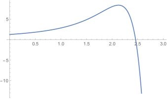
Figure 7: Plot of the nonlinear function $U(x)$

We infer that condition (4.164) actually prevents us from finding an equilibrium solution to the variational problem, and that is the main motivation to prove a verification theorem which avoids the use of the $C^{2}_{x}$ regularity of $V$ on all the continuation region of the other player. This observations clearly show how much the fitting conditions on ${\partial}F_{1}$ and ${\partial}F_{2}$ are interconnected and, in general, one must be careful to assume additional regularity on the value function on one side of $D$, so as not to run into inconsistencies with the conditions on the other half.

References

• [1] Aïd, R., Basei, M., Callegaro, G., Campi, L., and Vargiolu, T. Nonzero-sum stochastic differential games with impulse controls: a verification theorem with applications. Math. Oper. Res. 45, 1 (2020), 205–232.
• [2] Awerkin, A., and Vargiolu, T. Optimal installation of renewable electricity sources: the case of Italy. Decis. Econ. Finance 44, 2 (2021), 1179–1209.
• [3] Cai, C., and De Angelis, T. A change of variable formula with applications to multi-dimensional optimal stopping problems. Stochastic Process. Appl. 164 (2023), 33–61.
• [4] Cont, R., Guo, X., and Xu, R. Interbank lending with benchmark rates: Pareto optima for a class of singular control games. Math. Finance 31, 4 (2021), 1357–1393.
• [5] De Angelis, T., and Ferrari, G. Stochastic nonzero-sum games: a new connection between singular control and optimal stopping. Adv. in Appl. Probab. 50, 2 (2018), 347–372.
• [6] Guo, X., Tang, W., and Xu, R. A class of stochastic games and moving free boundary problems. SIAM J. Control Optim. 60, 2 (2022), 758–785.
• [7] Guo, X., and Xu, R. Stochastic games for fuel follower problem: $N$ versus mean field game. SIAM J. Control Optim. 57, 1 (2019), 659–692.
• [8] Karatzas, I., and Shreve, S. E. Brownian motion and stochastic calculus, second ed., vol. 113 of Graduate Texts in Mathematics. Springer-Verlag, New York, 1991.
• [9] Koch, T., and Vargiolu, T. Optimal installation of solar panels with price impact: a solvable singular stochastic control problem. SIAM J. Control Optim. 59, 4 (2021), 3068–3095.
• [10] Pascucci, A. PDE and martingale methods in option pricing, vol. 2 of Bocconi & Springer Series. Springer, Milan; Bocconi University Press, Milan, 2011.