Clearing the Air: Updated CS Fluorescence Efficiencies Don’t Solve the NUV/Sub-mm Cometary CS Abundance Discrepancy

Abstract

Observations of carbon monosulfide (CS), a possible photodissociation fragment of CS₂, has a long history serving as a remote proxy for atomic sulfur, and more broadly, one of the sulfur reservoirs in cometary bodies. Interpretations of CS fluorescence emissions in ultraviolet observations of comets have, to-date, relied on a murky and ill-documented lineage of calculations for CS fluorescence efficiencies that can be difficult to assess. We report new fluorescence efficiencies of the CS radical, utilizing a rovibrational structure with vibrational states up to $v=8$ and rotational states up to $N=100$. A new set of band transition rates is produced through benchmarking comparisons to laboratory electron impact experiments, and subsequently utilized in the fluorescence calculations. We confirm historical reports of the ultraviolet $(0,0)$ band fluorescence efficiency, and conclude that blends and an expanded rovibrational structure have little impact on the fluorescence properties. Combined, the present results affirm the accuracy of the historical record of sulfur abundances derived via ultraviolet CS emissions in cometary observations with e.g., IUE and HST. Benchmark comparisons to IUE observations of comet Bradfield show favorable agreement with the theoretical models. We expand the model to the time-domain, and find that thermalization of the ground state and/or ‘hot’ initial distributions of CS lead to noticable changes in the shape of the $(0,0)$ band. The impact on existing sulfur abundances derived via ultraviolet CS observations, and new connections to sulfur reservoirs in protoplanetary disks are discussed. The model code and computed fluorescence efficiencies are made publicly available.

1 Introduction

The astrochemical pathways leading to the formation of sulfur and sulfur-bearing species remain poorly understood. The abundance of atomic sulfur in the interstellar medium is nearly 1000 times larger than the abundances measured in molecular clouds and protoplanetary disks (Tieftrunk et al., 1994; Le Gal et al., 2019; Kama et al., 2019). One of the few sulfur-bearing molecules that has been detected in molecular clouds, protoplanetary disks, and our own solar system’s remnant planetesimals, like comets, is carbon monosulfide, or CS (Tieftrunk et al., 1994; Le Gal et al., 2019; Teague et al., 2018; Noonan et al., 2023, and sources therein). In astrophysical context the molecule is an important tracer of the C/O ratio within protoplanetary disks when observed in tandem with SO in the sub-mm (Keyte et al., 2023). While CS is commonplace in the planetary formation process, establishing its role and significance in the sulfur ecosystem remains a key goal for the field.

Observations of CS in astrophysical environments are typically made through two main methods: sub-millimeter (sub-mm) ro-vibrational transitions in the ground X${}^{1}\Sigma$ state and near-ultraviolet (NUV) fluorescence in the A${}^{1}\Pi$-X${}^{1}\Sigma$ system. These techniques have been applied to comets within our solar system to investigate potential precursor molecules, such as CS₂, OCS, and H₂CS. However, discrepancies often arise between the CS abundances determined from NUV and sub-mm observations of the same comet (Noonan et al., 2023; Biver et al., 2023). These variations complicate direct comparisons across different wavelengths and require an evaluation of the excitation efficiencies employed in calculating both the total molecular column densities and production rates. For sub-mm emissions, these can also be affected by collisions with other molecules, as well as excitation by thermal continua such as e.g. emission from the nucleus.

CS was first detected in comet C/1975 V1 (West) in 1975 (Smith et al., 1980) and to derive its general abundance, the authors calculated the fluorescence efficiency (or $g$-factor) of the NUV $(0,0)$ band, presumably with only one vibrational level in each electronic state, at a heliocentric/geocentric distance of 0.52 au. The following years saw investigations of the A-X band structure to derive a Boltzmann temperature of 70 K (Jackson et al., 1982), and found that the ratios of the $(0,0)$, $(1,0)$, and $(0,1)$ bands of the A-X system are well described by resonant fluorescence of solar radiation. The spatial alignment of S and CS emissions observed in comet C/1979 Y1 (Bradfield), as discussed in Sanzovo et al. (1993), suggested CS₂ as a parent molecule of CS due to its short lifetime and corresponding small scale length. Following this, Sanzovo et al. (1993) recalculated the $g$-factor for the CS A-X band and determined production rates for 15 comets. Subsequent papers referred to a fluorescence efficiency provided through a private communication with few details on how it was derived (e.g., Noll et al. 1995; Stern et al. 1998; Noonan et al. 2023). These derived $g$-factors are summarized in Table 1. Even for models that used the same solar reference spectrum, there is a variation of more than an order magnitude between the derived fluorescence efficiencies, and the effect of the comet’s orbital velocity with respect to the Sun on the fluorescence efficiency (Swing’s effect) has not been evaluated. As noted in Noonan et al. (2023), improved fluorescence efficiencies for the NUV bands of CS may contribute to a resolution of the NUV/sub-mm CS abundance discrepancies. To enhance the accuracy of CS column density measurements derived from NUV observations, it is necessary to rigorously evaluate the fluorescence efficiencies of the A${}^{1}\Pi$-X${}^{1}\Sigma$ bands.

Publication	Heliocentric	Solar Spectral	CS A${}^{1}\Pi$-X${}^{1}\Sigma$
	Distance (au)	Reference	$(0,0)$ $g$-factor (pho.-1 mol.-1 s-1)
Smith et al. (1980)	0.52	Malitson et al. (1960)	3.8 $\times$ 10-3
Jackson et al. (1982)	1.0	Kohl et al. (1978)	7 $\times$ 10-4
Sanzovo et al. (1993)	0.52	Kohl et al. (1978); A’Hearn et al. (1983)	3.9 $\times$ 10-3
Noll et al. (1995)	1.0	A’Hearn et al. (1983)	5.8 $\times$ 10-4
Stern et al. (1998)	1.0	A’Hearn et al. (1983)	5 $\times$ 10-4

Table 1: CS A${}^{1}\Pi$-X${}^{1}\Sigma$ $g$-factors from 1980 - Present

In this paper we perform new computational modeling of the fluorescing CS A${}^{1}\Pi$-X${}^{1}\Sigma$ system using the FlorPy code (Bromley et al., 2024), utilizing an updated set of transition rates benchmarked against an electron impact spectrum produced from e+CS₂ collisions. We review our modeling methodology, benchmarking experiment, and discuss for the first time the Swings effect for the CS A${}^{1}\Pi$-X${}^{1}\Sigma$ system. We conclude by reviewing astrophysical observations that can benefit from the improved model and review open questions as to the parentage of the CS radical.

2 Fluorescence Modeling

2.1 Theoretical Approach

Once an atom or molecule is produced in a cometary coma, the emitter begins to absorb and re-emit sunlight. Assuming a species is formed in the lowest energy (ground) state, absorptions of solar photons occur and re-distribute electron population amongst its energy levels. The level populations $n_{i}$ can be computed from a series of coupled equations written as

$$\frac{dn_{i}}{dt}=-n_{i}\sum^{N}_{i\neq{k}}(A_{i\rightarrow{k}}+{\rho}B_{i\rightarrow{k}})+\sum^{N}_{j\neq{i}}n_{j}(A_{j\rightarrow{i}}+{\rho}B_{j\rightarrow{i}})$$ (1)

where $A$ is the Einstein $A$ coefficient (the ‘transition rate’), $B$ are the Einstein coefficients for absorption and stimulated emission, and $\rho$ is the radiation field. We include $N$ individual levels in our model, resulting in $N$ equations and $N-1$ unknowns. After sufficient time, the level populations reach a steady-state called fluorescence equilibrium where $dn/dt=0$, and the system is completed by the replacement of one equation with the normalization condition $\sum_{i}n_{i}=1$ (Bromley et al., 2021; Magnani & A’Hearn, 1986; Bromley et al., 2024). The system of equations can be re-cast into matrix form, whose solution $n=A^{-1}\times{B}$ is tractable by numerous computational methods. From the level populations, the fluorescence efficiencies, or $g$-factors, are computed (in units of J s^-1 mol.^-1) as

$$g_{ji}=\frac{hc}{\lambda_{ji}}n_{j}A_{j\rightarrow{i}}$$ (2)

where $hc/\lambda_{ji}$ is the photon energy of the transition, $n_{j}$ is the equilibrium population of the upper level involved in the transition, and $A_{j\rightarrow{i}}$ is the transition rate. $g$-factors are also commonly reported in units of photons s^-1 mol.^-1, computed with the omission of $hc/\lambda$ in Eq. 2.

The fluorescence rate equations (Eq. 1) describe the level populations, assuming an environment dominated by photoabsorption and radiative decays. For atoms or molecule produced close to the nucleus, in the collisional part of a cometary coma, the species may thermalize to some degree with the neutral coma. For example, Jackson et al. (1982) found that the distribution of rotational states in CS, as inferred from high-resolution spectra of the NUV $(0,0)$ band, implied some degree of thermalization. This complication may impact the band luminosities of CS and contribute to the ongoing discrepancy between NUV and sub-mm-derived CS abundances.

The thermalization of the X${}^{1}\Sigma$ ground electronic state can be readily incorporated into Eq. 1. For a given rotational temperature $T_{\textrm{rot}}$, the (relative) level populations within X${}^{1}\Sigma$ can be computed as a Boltzmann distribution characterized by $T_{\textrm{rot}}$. Eq. 1 thus reduces to $N-m$ linearly coupled equations, where $N$ is the total number of levels, and $m$ is the number of known (constrained) levels described by $T_{\textrm{rot}}$. The matrix solution to the resulting $A\textrm{x}=B$ functional form, where $A$ is now an $m\times{m}$ matrix, can be similarly solved, where the known $n_{j}{\rho}B$ terms are incorporated into matrix $B$ in the ($N-m$) system of equations. In the present manuscript, we solve both the collision-free (Eq. 1) and partially-thermalized cases to investigate whether such effects dramatically alter the fluorescence properties of CS.

For the purposes of computing fluorescence efficiencies of CS, we utilize the Python-based fluorescence code ‘FlorPy’ described in Bromley et al. (2021, 2024). In practice, the rate equations are agnostic to the details of the atomic or molecular structure, and rely solely on transitions connecting levels described by their energies and total angular momenta $J$. Transitions themselves are described by a wavelength (or equivalently, an energy) with an associated transition rate in units of s^-1. Einstein B coefficients are computed from the Einstein $A$ coefficients. We utilize here the solar spectrum described in Bromley et al. (2024), where the fluxes pumping the A${}^{1}\Pi$-X${}^{1}\Sigma$ transitions of CS are from the re-calibration efforts described in Coddington et al. (2021), with the original high-resolution spectrum deriving from Hall & Anderson (1991). Pumping of the infrared transitions of CS is computed from high-resolution infrared spectra generated with the Planetary Spectrum Generator (PSG; Villanueva et al. 2018). The infrared solar spectrum utilized in the PSG derives from a series of high-resolution Fourier Transform Spectrometer measurements conducted by the ACE mission (Hase et al., 2010).

In Bromley et al. (2024) we presented a pipeline that was developed to produce fluorescence emission models of diatomic molecules, with particular application to CO⁺. This pipeline relied on existing molecular constants and employed the PGOPHER program (Western, 2017) to model the vibronic structure of the cation. We apply an analagous approach here to construct a line list of CS using molecular constants reported in Bergeman & Cossart (1981) and the PGOPHER program (Western, 2017) for the X${}^{1}\Sigma$ ground state and the first excited state A${}^{1}\Pi$. Within each electronic state, vibrational levels up to $v_{\textrm{max}}=8$ and rotational levels up to $N_{\textrm{max}}=100$ are retained. Within each vibrational level, we utilize the experimentally-derived constants for molecular rotation $(B)$ and the centrifugal distortion constants $D$. As noted by Bergeman & Cossart (1981), the A${}^{1}\Pi$-X${}^{1}\Sigma$ bands of CS are subject to substantial perturbations from interactions with other electronic states. In most reported laboratory and astronomical observations of CS in the ultraviolet, the spectral resolution does not permit clear separation between rotational lines, owing to the small rotational constants ($B\sim 0.8$ cm^-1). For simplicity, we also neglect perturbations as their impacts on the wavelengths are substantially smaller then that of the rotational constant $B$ without affecting the accuracy of the computed fluorescence efficiencies.

Previous calculations on diatomics relevant to cometary science demonstrated that including both rovibronic transitions between electronic states and rovibrational transitions within electronic states are required to accurately model the level populations (Magnani & A’Hearn, 1986; Schleicher, 2010; Bromley et al., 2024). In the present calculations, rovibronic transitions between all included vibrational levels of the X${}^{1}\Sigma$ and A${}^{1}\Pi$ electronic states are retained, as well as vibrational and rotational transitions within the X${}^{1}\Sigma$ ground state. Einstein $A$ coefficients for the transitions of CS are sourced from the calculations of Wei Xing & Sun (2020), and benchmarked against experimental measurements as described below. Energy level and transition line lists, which are used as inputs to the fluorescence model, are created from parsing the outputs of the PGOPHER calculations, which are built on the constants described previously and the newly-benchmarked transition rates, described further below.

2.2 Experimental Benchmarking

In the rate equations of fluorescence equilibrium, fluorescence efficiencies and their resulting band luminosities (produced by sums over each band’s transitions) depend on the transition rates. Further, fluorescence efficiencies and band luminosities are proportional to the Einstein $A$ coefficient (Eq. 2). Wei Xing & Sun (2020) noted significant discrepancies between computed lifetimes of CS vibrational levels and those reported from experimental efforts. To improve the accuracy of the computed data utilized in our models we re-normalized the theoretical lifetimes to the experimentally-measured lifetimes reported by Mahon et al. (1997), who used laser-induced fluorescence to selectively excite bands of CS and measure the resulting radiative lifetimes. For $v>4$, for which no measured radiative lifetimes are available, a linear fit ($R^{2}=0.997$) to the $v<4$ lifetimes of Mahon et al. (1997) is used to extrapolate out to higher $v$. The linear fit is used to predict experimental lifetimes for $v>4$, which are $\sim$30% larger than those originally reported in Wei Xing & Sun (2020).

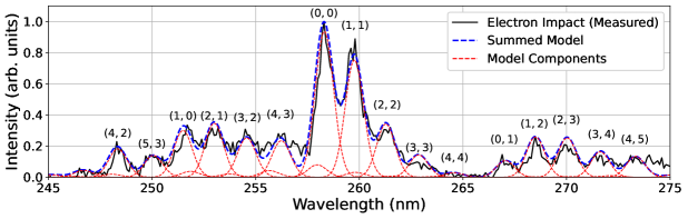
Figure 1: Comparison of the theoretical model (blue; summed over model components (red)) and electron impact spectrum produced by 100 eV electrons incident on CS₂ gas (black). Emission bands of the CS A${}^{1}\Pi$-X${}^{1}\Sigma$ system are labeled by $(v^{\prime},v^{\prime\prime})$, where $v^{\prime}$ and $v^{\prime\prime}$ are the upper and lower vibrational numbers, respectively. The modeled spectrum is generated from benchmarked transition rates and vibrational populations derived from the strongest feature associated with each A${}^{1}\Pi$ vibrational level. The electron impact spectrum is corrected for the sensitivity of the optical elements, and a minor wavelength shift is applied to the theoretical spectrum to account for wavelength calibration errors.

For a given vibrational level labeled by $v^{\prime}$, the branching ratios to lower vibrational levels, labeled by $v^{\prime\prime}$, are described by Franck-Condon factors. While these values are reported in various theoretical efforts, we opted to benchmark the relative transition rates (Franck-Condon factors) extracted from the tables of Wei Xing & Sun (2020) against experimental measurements. For this purpose, the emission spectrum of CS was recorded from crossed-beam electron impact experiments on CS₂ gas at the Laboratory of Electron Induced Fluorescence at Comenius University in Bratislava, Slovak Republic in Summer 2023. Details of the experimental apparatus are publicly available (see Danko et al. (2013); Bodewits et al. (2019); Bromley et al. (2024), and references therein). In short, an energy-monochromatized electron beam is crossed perpendicularly with a neutral beam of CS₂ gas inside a vacuum chamber (base pressure $\sim 10^{-8}$ mbar). Experiments were conducted in the single-collision regime with chamber pressures during gas injection not exceeding $10^{-4}$ mbar. Photons from decaying collision products (CS, CS₂, and CS${}_{2}^{+}$) were recorded by a Czerny-Turner monochromator equipped with a UV-sensitive photomultiplier tube. The optical response of the apparatus was established by previous measurements of a known system, H₂ $a^{3}\Sigma_{g}^{+}$-$b^{3}\Sigma_{u}^{+}$, and the thermal blackbody produced by a heated tungsten filament. An example of the resulting laboratory spectrum is shown in Figure 1 for a collision energy of 100 eV.

At electron energies above the threshold of CS (A${}^{1}\Pi$) formation from CS₂ ($\sim$9.27 eV), a large number of CS A${}^{1}\Pi$-X${}^{1}\Sigma$ bands are excited between 250 – 280 nm. Our observed relative intensities of the many CS bands agree well with those reported in Ajello & Srivastava (1981). In order to benchmark the vibrational transition rates reported in Wei Xing & Sun (2020), an iterative procedure was applied (described in the Appendix of Bromley et al. 2024). First, the relative intensities of all bands were extracted by either an integral over the spectral extent of each band, or in the case of strong blends (the case for most bands of CS), was manually adjusted to match the laboratory spectrum. To refine the handling of the many blended features, vibrational level populations are derived from the strongest bands of each A${}^{1}\Pi$ vibrational level, and manually adjusted to match the observed spectrum. The relative transition rates are then normalized to the lifetimes described above. We note that the rotational structure of the bands is not resolved, though the lifetimes appear weakly sensitive to the rotational quanta $J$ (Wei Xing & Sun, 2020). Further, for the purposes of the present benchmarking, a rotational temperature of $\sim$300 K was assumed. It is possible that the rotational distribution is non-thermal, but a more rigorous derivation of the rotational populations cannot be derived at the present spectral resolution. Lastly, the level populations are re-derived using the updated transition rates, and the process was repeated until sufficient agreement with the laboratory spectrum was achieved. In total, this process leads to changes of order 20 – 30% in transition rates of the strongest bands, and up to factors of $\sim$2 in weak transitions. Figure 1 shows a comparison of the laboratory spectrum at 100 eV electron energy and our final, benchmarked model built on the re-calibrated transition rates. The agreement with the experimental spectrum is excellent and lends confidence to our use of the benchmarked transition rates in computing fluorescence efficiencies.

3 Results

3.1 Band Luminosities

$v^{\prime}$ $\backslash$ $v^{\prime\prime}$	0	1	2
	257.77	266.51	275.77
0	5.02e-22	5.55e-23	1.55e-24
	6.52e-04	7.44e-05	2.16e-06
	250.94	259.21	267.96
1	1.76e-23	4.28e-23	1.29e-23
	2.23e-05	5.59e-05	1.74e-05
	244.58	252.44	260.72
2	8.39e-26	1.75e-24	1.68e-24
	1.03e-07	2.22e-06	2.20e-06

Table 2: Fluorescence Efficiencies of the CS (A${}^{1}\Pi$-X${}^{1}\Sigma$) bands at $r_{\textrm{h}}=1$ au and $v_{\textrm{h}}=0$ km s^-1. Fluorescence efficiencies are provided as a function of upper ($v^{\prime}$; rows) and lower ($v^{\prime\prime}$; columns) vibrational quantum numbers, respectively. For each band, the following values are provided (top to bottom): vacuum wavelength (nm) for the R(0) line within the band, the band luminosities (summed over all transitions) in units of Joules s^-1 molecule^-1, and band luminosities in units of photons s^-1 mol.^-1. Band luminosities for all bands (including $v^{\prime},v^{\prime\prime}>2$) are provided as supplementary files.

Previous fluorescence efficiencies of the A${}^{1}\Pi$-X${}^{1}\Sigma$ (0,0) band of CS range from $1\times 10^{-4}$ to $5.8\times 10^{-4}$ photons s^-1 mol.^-1 at a heliocentric distance of 1 au (Smith et al., 1980; Jackson et al., 1982; Noll et al., 1995; Stern et al., 1998) (see Table 1). As a first test of our model, we computed fluorescence efficiencies of the CS ultraviolet bands at a heliocentric distance of $r_{\textrm{h}}$ = 1 au and a heliocentric velocity of $v_{\textrm{h}}$ = 0 km s^-1. The resulting band luminosities, summed over the transitions in each band, are provided in Table 2. The luminosity of the $(0,0)$ band, $6.52\times 10^{-4}$ pho. s^-1 mol.^-1, is in good agreement with the value reported in Noll et al. (1995). Both Noll et al. (1995) and the present work utilize the molecular constants reported in Bergeman & Cossart (1981). However, the extent of the rovibrational structures utilized in the former is not clear. We find that bands from $v>2$ (not shown) have negligible band luminosities and are omitted from Table 2. The present values affirm that neither the updated solar spectrum, nor the large rovibrational level structure utilized here, have introduced large changes to the baseline g-factors.

As most UV comet observations have utilized low spectral resolution ($R\sim 1000$), the topic of blends must be addressed. In the laboratory, the strong $(0,0)$ band is blended with the neighboring $(1,1)$ band. In fluorescence, the equilibrium populations of the X${}^{1}\Sigma(v=1)$ rotational levels are small compared to $(v=0)$. Consequently, the fluorescence band luminosity of the $(1,1)$ band is less than 1/10^th that of the $(0,0)$ band, and the overlap between the bands is negligible. It can be concluded that any observed flux attributed to the CS $(0,0)$ band in comet observations is largely free of blends.

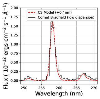
Figure 2: Present CS fluorescence model versus low-dispersion spectra of comet Bradfield (observation ID LWR 6008), collected on 10 Jan. 1980 at $r_{\textrm{h}}$ = 0.711 au (A’Hearn & Feldman, 1980). The NUV CS bands (left to right) $(1,0)$, $(0,0)$, and $(0,1)$ show good relative agreement with the fluorescence model.

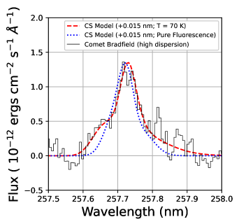
Figure 3: Present CS fluorescence models versus high-dispersion spectra of comet Bradfield (observation ID LWR 6757), collected on 24 Jan. 1980 at $r_{\textrm{h}}$ = 0.925 au (Jackson et al., 1982). The shape of the $(0,0)$ band is well described by the fluorescence model with fixed relative ground state populations described by $T=70$ K (Jackson et al., 1982).

Lastly, we consider the thermalization of the X${}^{1}\Sigma$ ground state. As CS is produced in the inner coma, it is plausible that the ground state populations are described by a Boltzmann distribution (Jackson et al., 1982). The NUV spectrum produced from pumping of a thermalized ground state population is likely to excite a wider range of transitions than pure fluorescence alone. We pursued calculations of band luminosities assuming ground state thermalization temperatures of 30, 70, 100, and 300 Kelvin. The resulting luminosities of the $(0,0)$ band differ by at most 4%, though the band shape can change dramatically with ground state temperature. Thus, for the purposes of deriving CS abundances, pure-fluorescence band luminosities are of sufficient accuracy.

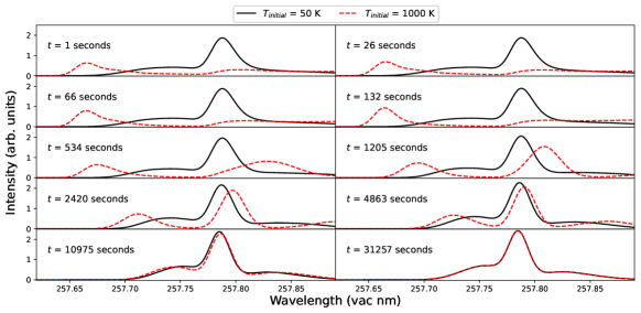
Figure 4: Computed spectrum of CS A${}^{1}\Pi$-X${}^{1}\Sigma~{}(0,0)$ from two time-dependent pure-fluorescence models with different initial conditions. Orbital conditions of $r_{\textrm{h}}=1$ au and $v_{\textrm{h}}=0$ km s^-1 are assumed. The two models utilize different initial conditions, where the levels at $t=0$ are given by Boltzmann distributions characterized by $T=50$ K (black curve) and $T=1000$ K (red curve). Transition-resolved $g$-factors are convolved with Gaussians with 0.02 nm FWHM to produce the presented profiles.

3.2 Cometary Spectra Benchmarks

As a benchmark test for these models, we apply them to both high and low dispersion spectra of comet Bradfield, collected with the International Ultraviolet Explorer (IUE). Figure 2 shows a comparison of the low-resolution IUE spectrum (LWR 6008, 1980 Jan. 10) of A’Hearn & Feldman (1980) at $r_{\textrm{h}}=0.711$ AU. Good agreement is observed between the cometary CS and the modeled spectra of the NUV $(0,0)$, $(0,1)$, and $(1,0)$ bands.

High-dispersion observations of Comet Bradfield, described in Jackson et al. (1982) were collected on 24 Jan. 1980. Figure 3 shows a comparison of the IUE spectra and our spectral modeling, assuming a ground state (X${}^{1}\Sigma$) temperature of 70 K. The agreement with the observed band shape is greatly improved in the thermalized ground state model when compared to pure fluorescence alone. An apparent deficiency in flux, red-ward of maximum intensity, remains apparent. A minor wavelength shift of +0.015 nm is also applied to the theoretical spectrum, assumed to correct for inaccuracies in the wavelength calibration of the high-dispersion IEU spectra. However, this shift may potentially indicate additional effects currently excluded from the present models.

CS is formed in the inner coma, where collisions are still important contributors to the excitation of CS. Molecular dissociation also tends to populate higher rotational states within the fragment molecule. Krishna Swamy & Tarafdar (1993) developed a theoretical emission model which explicitly included collisions between CS and H₂O in the rate equations. They computed the level populations time-dependently, assuming a constant outflow velocity, at conditions expected for comets Halley, Bradfield, and Giacobini-Zinner, as well as exploring different initial X${}^{1}\Sigma$ rotational populations expected from e.g. formation of CS from dissociation reactions. Comparisons to high-resolution spectra of 1P/Halley showed difficulties in matching the observed profiles. It is likely that the spectrum of CS, integrated over the inner coma, is sampling a distribution of CS that is still developing in time, likely from a non-thermal distribution(s) of initial X${}^{1}\Sigma$ rotational states. However, complications such as e.g. inaccurate molecular data or pointing/tracking difficulties during the IUE observations may also contribute to this problem (Krishna Swamy & Tarafdar, 1993). This appears to be less severe in comet Bradfield, with good agreement achieved between the observed low- and high-dispersion spectra and the present models which assume a thermal distribution for X${}^{1}\Sigma$. Additional models may be required to further explain the disagreements with high-resolution spectra of CS in 1P/Halley. These complications are discussed further below in the context of time-dependent fluorescence models.

3.3 Heliocentric Distance, Velocity, and Time-Dependent Effects

Once produced, CS has a comparable photochemical lifetime to H₂O, of order $10^{5}$ seconds against photoionization at 1 au (Meier & A’Hearn, 1997; Heays et al., 2017). The use of equilibrium fluorescence efficiencies in deriving accurate abundances from observed fluxes necessitates the validity of fluorescence equilibrium. We checked the validity of assuming fluorescence equilibrium by computing a time-dependent solution of the fluorescence rate equations (Eq. 1).

We utilize the time-dependent matrix method described previously in Bromley et al. (2024), assuming first that the CS is initially formed in the lowest energy state. From time-dependent calculations of the populations and $g$-factors, we find that the band luminosity of the $(0,0)$ evolves from a value $\sim 10\%$ greater than its equilibrium value at $t=0$, and asymptotically approaches within $5\%$ of the equilibrium fluorescence efficiency within $t=10^{3}-10^{4}$ seconds at 1 au. This suggests that any observed emission from CS initially produced in the ground rovibrational state is practically indistinguishable from a population of CS in fluorescence equilibrium.

CS₂, the often-attributed parent of CS (Noonan et al., 2023) produces CS in highly excited vibrational and rotational states upon photodissociation (McCrary et al., 1985). Krishna Swamy & Tarafdar (1993) found that such distributions relax toward fluorescence equilibrium much slower than CS initially formed in the ground rovibrational state. We explored similar possibilities in the present time-dependent models, assuming initial conditions described by Boltzmann distributions with a range of temperatures from 50 to 1000 K.

Figure 4 shows the time-evolution of the two extremes, where each population of CS is formed with X${}^{1}\Sigma$ levels described by a Boltzmann temperature of 50 K and 1000 K. The population of CS formed with $T=50$ K relaxes to fluorescence equilibrium rapidly. The population of CS formed at $T=1000$ K, for which the most-populated X${}^{1}\Sigma$ peaks around $J=20$, evolves to the same equilibrium over longer timescales of order $10^{4}$ seconds. The distribution of CS formed initially at 1000 K has apparent separation between the R branch (blueward of 257.7 nm) and the Q ($\sim$257.8 nm) and P (redward of 257.8 nm) branches. With increasing time, the two branches merge, with a noticeable peak increasing in intensity and shifting from the wavelength position of the P branch towards that seen in fluorescence equilibrium. If such a distribution were initially formed and evolving in the inner coma, one would expect a shift in the wavelength position in the peak flux, as was observed for comet Bradfield (Figs. 2-3).

Krishna Swamy & Tarafdar (1993) also noted a shift in the wavelength position of the peak flux in their time- and density-dependent models. As noted previously, an apparent wavelength shift of order 0.015 nm is apparent between the present fluorescence model and comparisons to the observed high-resolution IUE spectrum of comet Bradfield (Fig. 3). As this shift is several times larger than the spectral pixel width, it is likely that the wavelength shift is a real, physical effect, rather than a calibration error. From Krishna Swamy & Tarafdar (1993), these shifts may be caused by an out-of-equilibrium distribution of CS, which is being excited by both collisional and radiative processes in the inner coma. Visual inspection of Fig. 4, which shows instantaneous $g$-factors ($g(t)=hc/\lambda\times{n(t)}A$), exhibits a similar trend. When incorporated into density-dependent 3-dimensional models of cometary comae, integration over the appropriate line of sight may yield profiles similar to that observed in e.g. comets Halley and Bradfield, where CS in the inner coma is likely not in fluorescence equilibrium. While existing models assuming a thermalized ground state, such as those presented in Fig. 3 find good relative agreement with the observed spectra (assuming an arbitrary wavelength shift), additional work may be necessary to accurately describe the shape of the CS $(0,0)$ band. Further, additional work may be needed to understand whether the observed wavelength shifts confer information about as-yet-unidentified parent molecules through the initial distribution of rovibrational states populated upon photodissociation to CS.

As noted in the case of CO⁺ (Bromley et al., 2024), the variations in equilibrium band shapes are driven through competition of absorption rates between electronic states and radiative rovibrational transition rates within the ground electronic state. In the case of CS, the infrared transitions are relatively weak, with the strongest IR band, the X${}^{1}\Sigma$-X${}^{1}\Sigma$ ($1,0)$ band between 7.8 - 7.9 $\mu$m, having a band luminositiy $\sim{1}/100^{\textrm{th}}$ that of the A${}^{1}\Pi$-X${}^{1}\Sigma$ $(0,0)$ band. Thus CS is a weak infrared emitter. These trends are consistent with the weak dependence of the band shape on heliocentric distance (Fig. 6), discussed further below.

The absorption rates in the fluorescence rate equations (Eq. 1) depend on both heliocentric velocity and distance. Band luminosities may be insensitive to heliocentric distance while the distribution of features within a band can be affected dramatically, as was observed in e.g. CO⁺ (Bromley et al., 2024). Large variations in fluorescence efficiency— exceeding factors of two—with respect to heliocentric velocity have been observed in diatomics such as OH (Schleicher & A’Hearn, 1988) and CN (Schleicher, 2010). However, reports on how CS band luminosities vary with heliocentric velocity are currently lacking and we therefore explored the potential for similar trends in CS. Figure 5 shows the band luminosities of the two strongest A${}^{1}\Pi$-X${}^{1}\Sigma$ bands of CS as a function of heliocentric velocity. The band luminosity of the strong $(0,0)$ band is relatively insensitive to heliocentric velocities for $|v_{\textrm{h}}|<20$ km s^-1. At large heliocentric velocities $|v_{\textrm{h}}|>20$ km s^-1, variations in excess of 10% are apparent. The neighboring weak $(1,1)$ band appears insensitive to velocity, changing by at most 3% over the present velocity space of -50 to +50 km km s^-1, a reasonable parameter space for solar system comets.

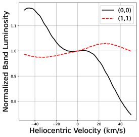
Figure 5: Heliocentric velocity dependencies of the two strongest ultraviolet A${}^{1}\Pi$-X${}^{1}\Sigma$ bands of CS. Each band is normalized to a value of 1 at $v_{\textrm{h}}=0$ km s^-1.

Similarly, previous studies have commonly adjusted the fluorescence efficiencies of CS from $r_{\textrm{h}}=1$ au by a factor of $1/r_{\textrm{h}}^{2}$. In some cases, such as CN (Schleicher, 2010), the band luminosities are sensitive to both heliocentric distance and velocity. As discussed previously, the NUV bands of CS are weakly sensitive to heliocentric velocity. To quantify the extent to which scaling $g$-factors from 1 au to $r_{\textrm{h}}$ is valid, we explicitly calculated the fluorescence efficiencies up to $r_{\textrm{h}}=10$ au. Within the range of typical heliocentric distances ($<$ few au) where UV observations have captured CS ultraviolet emission, the band luminosities changed by at most 2% between calculations re-scaled from 1 au, and those that explicitly account for the distance dependence of the absorption rates in the rate equations (Eq. 1). As shown in Fig. 6, changes in heliocentric distance can have a modest impact on the distribution of lines within a band. However, at the low spectral resolution with which CS has historically been observed ($\sim$0.5Å FWHM), the effect on the shape of the bands is negligible. In short, re-scaling of CS band luminosities from 1 au by a factor of $1/r_{\textrm{h}}^{2}$ for the purposes of deriving column densities and/or abundances is justified.

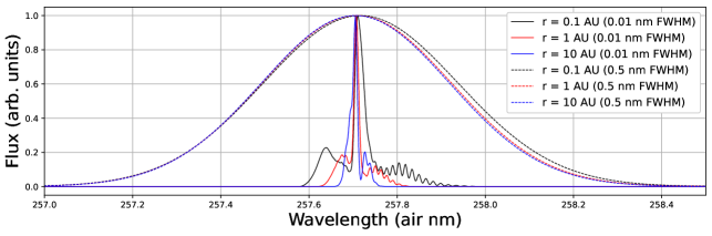
Figure 6: Synthetic fluorescence spectra of the CS ultraviolet $(0,0)$ band at $r_{\textrm{h}}=0.1,1,10$ au at high (0.01 nm FWHM, solid lines) and low (0.5 nm FWHM, dashed lines) spectral resolution. The vertical axis is proportional to J s^-1 mol^-1, with all models normalized to a maximum value of 1 to highlight changes to band shape.

4 Astrophysical Implications

The continued stability of the CS A${}^{1}\Pi$-X${}^{1}\Sigma$ fluorescence efficiencies, despite marked improvements in solar spectral references, an expanded rovibronic structure, and experimentally-benchmarked transition rates, confirms that the NUV-derived CS column densities in cometary comae from 1980 onward are accurate, even when the Swings effect was not explicitly accounted for. In turn, we are able to proceed in scrutinizing the cometary sulfur abundance catalog with renewed confidence in the measured column densities and production rates of CS, although the source of the molecule remains unclear (Meier & A’Hearn, 1997; Roth et al., 2021; Noonan et al., 2023). We note that our higher resolution calculations and ability to reliably calculate the Swings effect have implications for observations taken beyond the solar system, and in particular for protoplanetary disks.

As stated earlier, CS has been observed in protoplanetary disks frequently in the sub-mm, typically via the $J=2\rightarrow 1$ rotational transition (see for example Kama et al. 2019). As such, these observations probe the cold mid-plane of protoplanetary disks. NUV fluorescence of the CS molecule is extremely unlikely in this region due to the optically thick dust, preventing incident stellar radiation from exciting CS. Any CS fluorescence in the UV observed in protoplanetary disks would be linked to the upper layers of the disk, in the illuminated photodissociation region (Keyte et al., 2023). Despite many observations of protoplanetary disks encompassing the wavelength range of the CS A${}^{1}\Pi$-X${}^{1}\Sigma^{+}$ region as part of the ULYSSES survey (e.g., Arulanantham et al. 2018; Espaillat et al. 2022; Skinner & Audard 2022) we were unable to find any studies that confirmed the presence of this band. With the improved models for the CS $(0,0)$ band presented in this paper it may be possible to directly compare the abundances of CS in the midplane to CS that has been transported up into the PDR and is fluorescing. A similar strategy to capture the temperature structure in the disk has been employed by observing both the CO A${}^{1}\Pi$-X${}^{1}\Sigma^{+}$ band and the CO rovibrational lines at 4.7-5 $\mu$m (Arulanantham et al., 2018). Detections of the CS A${}^{1}\Pi$-X${}^{1}\Sigma$ band coincident with the sub-mm rotational emissions would provide insight into the variability of the S/O abundance as a function of vertical location in the disk. A systematic re-analysis of NUV observations of T-Tauri stars obtained with space telescopes like HST and IUE could produce such results.

This work was initiated following the identification of discrepancies in sulfur abundances derived from sub-mm and UV observations of comets, as discussed in Noonan et al. (2023). A possible source of these discrepancies, inaccurate fluorescence efficiencies for the NUV bands of CS, has now been ruled out. The present $g$-factors, utilizing a greatly expanded solar spectrum, energy level structure, and experimentally-benchmarked transition rates, recovers comparable $g$-factors to previous studies of the molecule. However, additional factors may contribute to the ongoing disrepancies between NUV- and sub-mm-derived CS abundances:

• The current state-of-the-art photochemical lifetime data for CS is purely theoretical (e.g. Heays et al. 2017), and large errors in the photodissociation and/or photoionization lifetimes may lead to either enhanced or substantially reduced CS abundances.

• Submillimeter observations probe the very innermost coma where collisional effects are important; these may severely complicate a fluorescence efficiency calculation for the rotational transitions of CS.

• As noted in Noonan et al. (2023), CS₂ alone can not explain the abundance of CS inferred from UV observations. Prompt emission of CS following dissociation from possibly unidentified parent species could contribute to either NUV or sub-mm emission features, complicating a derivation of the CS abundances. Further, prompt emission populates a different array of rovibrational states, with typically higher rotational states compared to solar fluroescence (see e.g. the case of OH in A’Hearn et al. 2015). These highly-excited states evolve differently in time compared to molecules formed in the ground rovibrational state, which can present a substantial challenge for accurate spectral modeling. High-resolution UV comet spectra, capable of spectrally separating the rotational transitions within the $(0,0)$ band would directly test this possibility, and could theoretically be carried out using the G230H Echelle grating for the HST’s STIS instrument (R$\sim$114,000). However, the low throughput and narrow slit size would require that the target be both unusually bright and have a well-characterized orbit to minimize acquisition errors.

5 Conclusions

The historical record of CS A${}^{1}\Pi$-X${}^{1}\Sigma$ fluorescence efficiencies covers a range of reported values, with minimal description of the molecular and solar data used in their production. As such, the confidence in existing column densities and abundances of CS derived via UV observations of the $(0,0)$ was unclear. We reported new fluorescence efficiency calculations of the CS radical utilizing a large rovibronic structure and a new set of experimentally benchmarked transition rates. The present $g$-factor for the UV A-X $(0,0)$ band at $\sim$2580 Å, $6.52\times 10^{-4}$ photons sec.^-1 mol.^-1, is consistent with previous literature and suggests changes in derived CS abundances of $\leq 11\%$.

Concluding, we find that the extent of the rovibronic structure utilized in the calculations has a negligible impact on the fluorescence efficiency of the strongest systems. We report, for the first time, explicit calculation of the Swings effect for CS, and find that the bands are weakly sensitive to the heliocentric velocity of the emitting environment. In addition, the band shape changes negligibly as a function of $r_{\textrm{h}}$, and scaling of $g$-factors at 1 au to a given heliocentric distance via $1/r_{\textrm{h}}^{2}$ is valid. Thermalization of the X${}^{1}\Sigma$ ground state leads to observable changes in band shape, as realized in archived IUE comet spectra. However, this effect changes band the luminosities by only a few per cent compared to the pure-fluorescence models, and does not impact any previously derived CS abundances.

From time-dependent propagation of the fluorescence equations, we find that CS initially formed in the ground rovibrational state quickly achieves fluorescence equilibrium, suggesting that the use of $g$-factors computed with the assumption of fluorescence equilibrium has not introduced large errors in existing abundance derivations. However, time-dependent models with a ‘hot’ distribution of CS, formed initially at $T=1000$ K evolves much differently in time and produces similar band luminosities. The time-dependent modeling suggests that observed wavelength shifts between the theoretical models and IUE cometary spectra are consistent with CS being formed in a variety of rovibrational states. Additional modeling, incorporating collisional (density-dependent) effects may be necessary to fully explain the observed band shapes of the CS $(0,0)$ band in the NUV. Further, more refined modeling may provide insights into the possible parents of CS through an understanding of the initial rovibrational states of CS populated by photodissociation of parent molecules. A possible observing schema with HST is noted which could provide sufficient spectral resolution to investigate possible CS prompt emission.

We describe possible avenues for investigating sulfur reservoirs in protoplanetary disks via UV fluorescence of the CS ultraviolet A-X $(0,0)$ band. Such analyses may shed light on the temperature structure in the disk via comparisons of archival sub-mm and UV observations in the midplane and photodissociation regions. Lastly, we note that inaccurate molecular data for photodissociation or photoionization of CS, collisional effects, or prompt emission from unidentified parent species may dramatically complicate the interpretation of CS abundances derived from NUV or sub-mm observations of comets.

We hope that the calculations presented here will be used to further investigate the discrepancies between NUV- and sub-mm-derived sulfur abundances in cometary observations. The fluorescence model, input files, fluorescence efficiencies, and related supplementary files are provided on the Zenodo service (https://zenodo.org/records/12555642).

References

- A’Hearn & Feldman (1980) A’Hearn, M. F., & Feldman, P. D. 1980, The Astrophysical Journal Letters, 242, L187, doi: 10.1086/183429
- A’Hearn et al. (2015) A’Hearn, M. F., Krishna Swamy, K. S., Wellnitz, D. D., & Meier, R. 2015, The Astronomical Journal, 150, 5, doi: 10.1088/0004-6256/150/1/5
- A’Hearn et al. (1983) A’Hearn, M. F., Ohlmacher, J. T., & Schleicher, D. G. 1983, A high resolution solar atlas for fluorescence calculations, Univ. of Maryland Astronomy Program Technical Report TR AP83-044 (1983)
- Ajello & Srivastava (1981) Ajello, J. M., & Srivastava, S. K. 1981, The Journal of Chemical Physics, 75, 4454, doi: 10.1063/1.442612
- Arulanantham et al. (2018) Arulanantham, N., France, K., Hoadley, K., et al. 2018, The Astrophysical Journal, 855, 98
- Bergeman & Cossart (1981) Bergeman, T., & Cossart, D. 1981, Journal of Molecular Spectroscopy, 87, 119, doi: https://doi.org/10.1016/0022-2852(81)90088-6
- Biver et al. (2023) Biver, N., Bockelée-Morvan, D., Crovisier, J., et al. 2023, Astronomy & Astrophysics, 672, A170, doi: 10.1051/0004-6361/202245672
- Bodewits et al. (2019) Bodewits, D., Országh, J., Noonan, J., Ďurian, M., & Matejčík, S. 2019, The Astrophysical Journal, 885, 167, doi: 10.3847/1538-4357/ab43c9
- Bromley et al. (2021) Bromley, S., Neff, B., Loch, S., et al. 2021, The Planetary Science Journal, 2, 228, doi: 10.3847/psj/ac2dff
- Bromley et al. (2024) Bromley, S. J., Noonan, J. W., Cochran, A. L., et al. 2024, Monthly Notices of the Royal Astronomical Society, 528, 7358, doi: 10.1093/mnras/stae456
- Coddington et al. (2021) Coddington, O. M., Richard, E. C., Harber, D., et al. 2021, Geophysical Research Letters, 48, e2020GL091709, doi: https://doi.org/10.1029/2020GL091709
- Danko et al. (2013) Danko, M., Orszagh, J., Ďurian, M., et al. 2013, Journal of Physics B: Atomic, Molecular and Optical Physics, 46, 045203, doi: 10.1088/0953-4075/46/4/045203
- Espaillat et al. (2022) Espaillat, C., Herczeg, G. J., Thanathibodee, T., et al. 2022, The Astronomical Journal, 163, 114
- Hall & Anderson (1991) Hall, L. A., & Anderson, G. P. 1991, Journal of Geophysical Research: Atmospheres, 96, 12927, doi: https://doi.org/10.1029/91JD01111
- Hase et al. (2010) Hase, F., Wallace, L., McLeod, S. D., Harrison, J. J., & Bernath, P. F. 2010, Journal of Quantitative Spectroscopy and Radiative Transfer, 111, 521, doi: https://doi.org/10.1016/j.jqsrt.2009.10.020
- Heays et al. (2017) Heays, A. N., Bosman, A. D., & van Dishoeck, E. F. 2017, Astronomy & Astrophysics, 602, A105, doi: 10.1051/0004-6361/201628742
- Jackson et al. (1982) Jackson, W., Halpern, J., Feldman, P., & Rahe, J. 1982, Astronomy and Astrophysics, 107, 385
- Kama et al. (2019) Kama, M., Shorttle, O., Jermyn, A. S., et al. 2019, The Astrophysical Journal, 885, 114
- Keyte et al. (2023) Keyte, L., Kama, M., Booth, A. S., et al. 2023, Nature Astronomy, doi: 10.1038/s41550-023-01951-9
- Kohl et al. (1978) Kohl, J. L., Parkinson, W. H., & Kurucz, R. L. 1978, Center and limb solar spectrum in high spectral resolution 225.2 NM to 319.6 NM