High-order Adaptive Rank Integrators for Multi-scale Linear Kinetic Transport Equations in the Hierarchical Tucker Format

Abstract

In this paper, we present a new adaptive rank approximation technique for computing solutions to the high-dimensional linear kinetic transport equation. The approach we propose is based on a macro-micro decomposition of the kinetic model in which the angular domain is discretized with a tensor product quadrature rule under the discrete ordinates method. To address the challenges associated with the curse of dimensionality, the proposed low-rank method is cast in the framework of the hierarchical Tucker decomposition. The adaptive rank integrators we propose are built upon high-order discretizations for both time and space. In particular, this work considers implicit-explicit discretizations for time and finite-difference weighted-essentially non-oscillatory discretizations for space. The high-order singular value decomposition is used to perform low-rank truncation of the high-dimensional time-dependent distribution function. The methods are applied to several benchmark problems, where we compare the solution quality and measure compression achieved by the adaptive rank methods against their corresponding full-grid methods. We also demonstrate the benefits of high-order discretizations in the proposed low-rank framework.

35Q85, 65F55, 65L04, 65M06, 65M50

1 Introduction

Simulating linear kinetic transport equations is critical to understanding physical processes found in diverse disciplines such as nuclear engineering, astrophysics, and computational medicine. Kinetic models for transport capture the evolution of a high-dimensional probability density function $f\left(\mathbf{x},\mathbf{\Omega},t\right)$ which represents the probability of finding a particle, such as a neutron or photon, at position $\mathbf{x}\in\mathbb{R}^{d}$, moving in the direction $\mathbf{\Omega}\in\mathbb{S}^{d-1}$, at time $t$. The storage of the distribution function in the fully discrete setting is known to suffer from the curse of dimensionality. This issue is further compounded by the need to resolve multi-scale effects such as collisions with other particles and interactions with the background material. Depending on the relative importance of the terms, the equations can also change type in different physical regimes. In these circumstances, naive discretization techniques can become inefficient because of highly restrictive stability conditions or inaccurate due to physical inconsistencies associated with approximate models. These characteristics have motivated the development of asymptotic preserving (AP) methods which capture the macroscopic behavior at the discrete level.

The technical report by Brunner [4] provides an excellent overview of several classes of numerical methods for transport problems, including Monte Carlo methods, discrete ordinates methods, and moment methods based on expansions in the spherical harmonic basis. Monte Carlo methods [47, 10, 32], which track the evolution of particles along characteristics, are conceptually simple and relatively efficient to parallelize. However, these methods require many simulation particles to combat statistical noise, and the solution quality degrades in more rarefied regions where fewer particles are present. The discrete ordinates ($S_{N}$) [39, 2] method restricts the angular component of the distribution function to a collection of directions taken from the unit sphere. In spite of their efficiency, their primary disadvantages are that they introduce numerical artifacts such as ray effects, and the angular discretization does not preserve rotational invariance of the solution. On the other hand, moment discretizations with spherical harmonics [38] preserve the rotational invariance, but encounter challenges in highly kinetic regions, as the quality of the spectral approximation degrades in the presence of angular discontinuities [38]. Filtered spherical harmonics methods [37, 18] can improve the quality of the solutions, but many challenges remain such as the enforcement of more general boundary conditions. Adaptive sparse grid representations based on tensor products of wavelets have also been considered as a way to address the high dimensionality in kinetic simulations [20, 21, 22]. In these approaches, wavelet approximations are used to represent functions on hierarchical meshes with compact basis functions obtained through scaling and translation properties. Another interesting approach was proposed by Zhang et al.[48] in which the semi-Lagrangian method was used to remove the stiffness of convection terms in the intermediate regimes, resulting in a method with uniform unconditional stability. Peng et al.[41] recently proposed a reduced basis method for the linear transport equation that constructs subspaces for the components of the macro-micro decomposition using an efficient iterative algorithm, which also respects the diffusion limit.

Adaptive rank integrators, such as the dynamical low-rank (DLR) and step-and-truncate (SAT) methods, have emerged as a popular tool for accelerating the solution of high-dimensional kinetic equations and reducing their memory footprint [30, 16, 25, 23, 12]. Application of these methods to problems of interest in the transport community is fairly recent. In [44], Peng et al.developed a low-rank scheme for moment models of transport using spherical harmonics angular discretizations. These ideas were later used to develop high-order-low-order schemes that evolve the high fidelity model using a low-rank scheme that is used to define a closure to a fluid system [42]. Ding et al.[11] analyzed the behavior of DLR methods in the diffusive regime of the linear transport equation, and they showed that low-rank methods are capable of capturing such limits. Einkemmer et al.[14] proposed a DLR method for the linear transport equation which is AP and can be second-order accurate in both time and space. Their low-rank scheme is built on the macro-micro decomposition and staggered grid discretization originally proposed by Lemou and Mieussens [35]. A similar macro-micro decomposition strategy was later applied to the BGK equation in the collisional setting to enforce the limiting Navier-Stokes equations [15] and, more recently, the Lenard-Bernstein equation [8]. Peng and McClarren proposed a low-rank scheme which is first-order accurate in both time and space [43], using the $S_{N}$ method. Their approach applies a low-rank discretization to each octant of the sphere which is evolved using a transport sweep with source iteration. In [28], Hu and Wang presented an adaptive low-rank scheme for the nonlinear Boltzmann equation and combined this with a Fourier spectral method to approximate the collision operator. An energy stable DLR scheme for transport problems was recently proposed by Einkemmer et al.[13] based on the spherical harmonics discretization of the angular domain. Using a certain time step restriction, they showed that the resulting scheme obeyed an energy dissipation principle.

The majority of the aforementioned approaches use a projector splitting technique [36, 17] or the “unconventional” basis update Galerkin (BUG) integrator [7] to update the low-rank basis independently. A limitation of these earlier approaches is that they require a fixed rank, although, recently, extensions of the BUG integrator have been proposed to promote rank adaptivity [6, 27]. In contrast, the adaptive rank SAT framework [24] avoids the projector splitting used by the DLR approach and can be combined with traditional high-order numerical discretizations, such as the one proposed in [29]. Additionally, the SAT framework provides considerable flexibility in the arrangement of the dimension trees used to represent tensors. In this paper, we represent high-dimensional functions using the HTT format [26, 19], which has been proven to be effective in taming the challenges associated with the curse of dimensionality in kinetic simulations. We achieve notable improvements in efficiency through the use of a high-order singular value decomposition (HOSVD) compression, which is used to truncate nodes of the dimension tree with small singular values.

This work contributes several novel low-rank approximation techniques for solving the high-dimensional linear kinetic transport equation. Our approach utilizes a macro-micro decomposition of the distribution function in the kinetic model, which ensuring the scheme recovers the limiting linear diffusion equation under the appropriate scalings. The proposed methods support rank adaptivity, address the curse of dimensionality using the HTT format, and are based on a traditional high-order methods. The discretization of space is performed using a high-order weighted essentially non-oscillatory (WENO) finite-difference method, while the temporal discretization is performed using high-order implicit-explicit (IMEX) Runge-Kutta (RK) methods with the globally stiffly accurate (GSA) property to handle the stiffness associated with the diffusion limit. The discretization of the angular domain is performed using the $S_{N}$ method. In this work, we consider the Chebyshev-Legendre (CL) quadrature nodes, which form a tensor product quadrature rule on the surface of the unit sphere. We also introduce a projection technique to enforce a condition on the zeroth angular moment of $g$ that is fundamental to the macro-micro decomposition. Additionally, we discuss the evaluation of Hadamard products, which are crucial in transport applications to capture interactions with the background material, and highlight the computational challenges associated with these terms in the low-rank setting. Our numerical results demonstrate the capabilities of the proposed methods on two example problems from the transport literature. The first example considers a strongly varying scattering-cross section, which combines characteristics of both free-streaming and collisional regimes, and the second is a modification of the lattice problem, which contains discontinuities in material cross-sections. The low-rank structures present in these benchmark problems are carefully examined by studying the growth in the hierarchical rank and the decay of the singular values at the nodes of the tensor trees. We find that the proposed methods can significantly reduce the storage requirements.

The organization of the remainder of this paper begins with an overview of the problem formulation in Section 2. In Section 3, we provide the relevant details of the discretization adopted by the proposed methods. We begin with the time discretization for the system, before moving to the discretization of the angular domain, and then treat the spatial domain. Then, we connect these elements to the HTT format and address some complications relevant to transport applications. Section 4 presents the numerical results which considers several benchmark problems from the literature. We conclude the paper with a brief summary in Section 5.

2 The Linear Transport Equation and Macro-micro Decomposition

We consider the time-dependent linear transport equation under a diffusive scaling:

(1) $$\partial_{t}f+\frac{1}{\epsilon}\mathbf{\Omega}\cdot\nabla_{x}f=\frac{\sigma_{s}}{\epsilon^{2}}\Big{(}\langle f\rangle_{\mathbf{\Omega}}-f\Big{)}-\sigma_{a}f+Q,\quad(\mathbf{x},\mathbf{\Omega})\in D\times\mathbb{S}^{2},$$

where $D\subset\mathbb{R}^{2}$ in this work, and $\mathbb{S}^{2}$ is the surface of the unit sphere. Additionally, we let $\sigma_{a}\left(\mathbf{x}\right)\geq 0$ and $\sigma_{s}\left(\mathbf{x}\right)>0$ denote the absorption and scattering cross-sections for the background material and $Q(\mathbf{x},t)$ is the radiant source. Additionally, the Knudsen number $\epsilon$ characterizes the strength of the collisions in the problem. In this work, we only consider isotropic collisions, so the relevant collision operator consists of integration over the unit sphere, specifically

$$\langle f\rangle_{\mathbf{\Omega}}:=\frac{1}{4\pi}\int_{\mathbb{S}^{2}}f\left(\mathbf{x},\mathbf{\Omega}^{\prime},t\right)\,d\mathbf{\Omega}^{\prime}.$$

Although it is more conventional to use inflow-outflow type boundary conditions, we shall restrict ourselves to periodic domains and leave the complication of boundary conditions to future work.

One of the challenges associated with the kinetic model (1) is the capturing the range of behavior observed as $\epsilon$ changes. When $\epsilon=\mathcal{O}(1)$, the kinetic equation behaves as a hyperbolic equation, but transitions to a parabolic or diffusive regime when $\epsilon\ll 1$. Lemou and Mieussens [35] proposed the macro-micro decomposition, which separates $f$ into an equilibrium and non-equilibrium components, namely

(2) $$f\left(\mathbf{x},\mathbf{\Omega},t\right)=\rho\left(\mathbf{x},t\right)+\epsilon g\left(\mathbf{x},\mathbf{\Omega},t\right),$$

where $\rho=\langle f\rangle_{\mathbf{\Omega}}$, and we have the condition $\langle g\rangle_{\mathbf{\Omega}}=0$. Using the decomposition (2), it can be shown that the linear kinetic equation (1) is equivalent to the system

(3) $$\partial_{t}\rho+\nabla_{x}\cdot\left(\left\langle\mathbf{\Omega}g\right\rangle_{\mathbf{\Omega}}\right)=-\sigma_{a}\rho+Q,$$

(4) $$\partial_{t}g+\frac{1}{\epsilon}\Big{(}I-\Pi\Big{)}\Big{(}\nabla_{x}\cdot\left(\mathbf{\Omega}g\right)\Big{)}+\frac{1}{\epsilon^{2}}\nabla_{x}\cdot\left(\mathbf{\Omega}\rho\right)=-\frac{\sigma_{s}}{\epsilon^{2}}g-\sigma_{a}g,$$

where $I$ is the identity operator, and we use the notation

$$\Big{(}I-\Pi\Big{)}\Big{(}\nabla_{x}\cdot\left(\mathbf{\Omega}g\right)\Big{)}:=\nabla_{x}\cdot\left(\mathbf{\Omega}g\right)-\nabla_{x}\cdot\left(\left\langle\mathbf{\Omega}g\right\rangle_{\mathbf{\Omega}}\right).$$

In the limit $\epsilon\rightarrow 0$ the macro-micro system (3)-(4) recovers the diffusion limit of the kinetic model (1). At the leading order, equation (4) reduces to

$$g=-\frac{1}{\sigma_{s}}\Omega\cdot\nabla_{x}\rho.$$

Then, substituting this result into the macroscopic equation (3) and using the identity $\left\langle\mathbf{\Omega}\otimes\mathbf{\Omega}\right\rangle_{\mathbf{\Omega}}=I/3$, one obtains the linear diffusion equation

$$\partial_{t}\rho-\nabla_{x}\cdot\left(\frac{1}{3\sigma_{s}}\nabla_{x}\rho\right)=-\sigma_{a}\rho+Q.$$

Therefore, the macro-micro system (3)-(4) relaxes to the same asymptotic limit of the kinetic equation (1) obtained from a Chapman-Enskog expansion.

3 Discretization of the Macro-micro System

This section provides details for the discretization of the macro-micro system used to build the proposed low-rank methods. We first discuss the IMEX-RK discretization for problems with relaxations, before introducing the discrete ordinates method and the tensor product angular discretization. Two different dimension trees are presented for representing tensors, and their interplay with the various discretizations is discussed. Projection techniques are introduced to enforce physical constraints in the proposed low-rank methods. Finally, we highlight the complications created by element-wise products between the material cross-sections and solution tensors.

3.1 IMEX Time Discretizations

Due to the stiffness associated with the diffusion limit of the system system (3)-(4), we shall restrict the discussion to IMEX discretizations with the GSA property [3]. It is customary to treat terms of $\mathcal{O}(1/\epsilon^{2})$ implicitly while those of size $o(1/\epsilon^{2})$ are treated explicitly, as the former will become extremely stiff in the limit $\epsilon\rightarrow 0$. The basic building block is the first-order accurate semi-discrete system

(5) $$\rho^{n+1}=\rho^{n}-\Delta t\nabla_{x}\cdot\left(\left\langle\mathbf{\Omega}g^{n}\right\rangle_{\mathbf{\Omega}}\right)-\Delta t\sigma_{a}\rho^{n}+\Delta tQ^{n},$$

(6) $$g^{n+1}=g^{n}-\frac{\Delta t}{\epsilon}\Big{(}I-\Pi\Big{)}\Big{(}\nabla_{x}\cdot\left(\mathbf{\Omega}g^{n}\right)\Big{)}-\frac{\Delta t}{\epsilon^{2}}\nabla_{x}\cdot\left(\mathbf{\Omega}\rho^{n+1}\right)-\frac{\Delta t\sigma_{s}}{\epsilon^{2}}g^{n+1}-\sigma_{a}\Delta tg^{n}.$$

We remark that in the limit $\epsilon\rightarrow 0$, equation (5) tends to an explicit discretization of a linear diffusion equation. Using algebra, the solution $g^{n+1}$ in the second equation (6) is found to be

$$g^{n+1}=\frac{1}{\epsilon^{2}+\Delta t\sigma_{s}}\Bigg{[}\epsilon^{2}g^{n}-\epsilon\Delta t\Big{(}I-\Pi\Big{)}\Big{(}\nabla_{x}\cdot\left(\mathbf{\Omega}g^{n}\right)\Big{)}-\Delta t\nabla_{x}\cdot\left(\mathbf{\Omega}\rho^{n+1}\right)-\epsilon^{2}\Delta t\sigma_{a}g^{n}\Bigg{]}.$$

Note that the coefficient multiplying the terms in brackets is spatially dependent, in the general case, and its action is defined point-wise. This form of the macroscopic equation is used in practice, although the form (6) is more convenient for the application of higher-order IMEX schemes, which we now describe.

IMEX-RK schemes of higher order can be represented by two Butcher tables [1]

(7)

$$\widetilde{\mathbf{c}}$$

      

where the matrix $\widetilde{A}$ represents the explicit part of the discretization, so $\widetilde{a}_{ij}=0$, for $j\geq i$. Its implicit counterpart $A$ is assumed to be lower triangular so that $a_{ij}=0$, when $j>i$. Additionally, the entries of the coefficient vectors are defined as

$$\widetilde{c}_{i}=\sum_{j=1}^{i-1}\widetilde{a}_{ij},\quad c_{i}=\sum_{j=1}^{i}a_{ij},\quad i=1,2,\cdots,s.$$

The vectors $\widetilde{\mathbf{b}}$ and $\mathbf{b}$ represent the quadrature weights for the stages of the RK scheme.

Applying the IMEX-RK discretization to the system (3)-(4), we obtain the following semi-discrete formulation:

(8) $$\rho^{n+1} =\rho^{n}+\Delta t\sum_{\ell=1}^{s}\widetilde{b}_{\ell}\Bigg{(}-\nabla_{x}\cdot\left(\left\langle\mathbf{\Omega}g^{(\ell)}\right\rangle_{\mathbf{\Omega}}\right)-\sigma_{a}\rho^{(\ell)}+Q^{(\ell)}\Bigg{)},$$

(9) $$g^{n+1} =g^{n}-\frac{\Delta t}{\epsilon}\sum_{\ell=1}^{s}\widetilde{b}_{\ell}\Big{(}I-\Pi\Big{)}\Big{(}\nabla_{x}\cdot\left(\mathbf{\Omega}g^{(\ell)}\right)\Big{)}$$

$$\qquad-\Delta t\sum_{\ell=1}^{s}\widetilde{b}_{\ell}\sigma_{a}g^{(\ell)}-\frac{\Delta t}{\epsilon^{2}}\sum_{\ell=1}^{s}b_{\ell}\Big{(}\nabla_{x}\cdot\left(\mathbf{\Omega}\rho^{(\ell)}\right)+\sigma_{s}g^{(\ell)}\Big{)}.$$

The values of $\rho^{(\ell)}$ and $g^{(\ell)}$ in each stage $\ell=1,2,\cdots,s$ are calculated as

(10) $$\rho^{(\ell)} =\rho^{n}+\Delta t\sum_{j=1}^{\ell-1}\widetilde{a}_{\ell j}\Big{(}-\nabla_{x}\cdot\left(\left\langle\mathbf{\Omega}g^{(j)}\right\rangle_{\mathbf{\Omega}}\right)-\sigma_{a}\rho^{(j)}+Q^{(j)}\Big{)},$$

(11) $$g^{(\ell)} =g^{n}-\frac{\Delta t}{\epsilon}\sum_{j=1}^{\ell-1}\widetilde{a}_{\ell j}\Big{(}I-\Pi\Big{)}\Big{(}\nabla_{x}\cdot\left(\mathbf{\Omega}g^{(j)}\right)\Big{)}$$

$$\qquad-\Delta t\sum_{j=1}^{\ell-1}\widetilde{a}_{\ell j}\sigma_{a}g^{(j)}-\frac{\Delta t}{\epsilon^{2}}\sum_{j=1}^{\ell}a_{\ell j}\Bigg{(}\nabla_{x}\cdot\left(\mathbf{\Omega}\rho^{(j)}\right)+\sigma_{s}g^{(j)}\Bigg{)}.$$

Schemes that are GSA have the property that the numerical solution at $t^{n+1}$ is equivalent to the last internal stage of the RK method [9], so it follows that

$$\rho^{n+1}=\rho^{(s)},\quad g^{n+1}=g^{(s)}.$$

We remark that the solution of equation (11) at each stage $\ell=1,2,\cdots,s$ is

$$g^{(\ell)}=\frac{1}{\epsilon^{2}+a_{\ell\ell}\Delta t\sigma_{s}}\Bigg{[}\epsilon^{2}g^{n}-\epsilon\Delta t\sum_{j=1}^{\ell-1}\widetilde{a}_{\ell j}\Big{(}I-\Pi\Big{)}\Big{(}\nabla_{x}\cdot\left(\mathbf{\Omega}g^{(j)}\right)\Big{)}-\epsilon^{2}\Delta t\sum_{j=1}^{\ell-1}\widetilde{a}_{\ell j}\sigma_{a}g^{(j)}\\ -\Delta t\sum_{j=1}^{\ell}a_{\ell j}\nabla_{x}\cdot\left(\mathbf{\Omega}\rho^{(j)}\right)-\epsilon^{2}\Delta t\sum_{j=1}^{\ell-1}a_{\ell j}\sigma_{s}g^{(j)}\Bigg{]}.$$

3.2 Angular Discretization

In this work, we shall consider tensor product quadrature rules on the unit sphere in the framework of the $S_{N}$ method. The $S_{N}$ method approximates the angular dependence of the solution at a fixed collection of points on the unit sphere $\mathbb{S}^{2}$. Recall that the unit vector $\mathbf{\Omega}\in\mathbb{S}^{2}$ can be defined in spherical coordinates as

$$\mathbf{\Omega}=\Big{(}\cos(\theta)\sin(\phi),\sin(\theta)\sin(\phi),\cos(\phi)\Big{)},$$

where $\theta\in[0,2\pi)$ is the azimuthal angle, and $\phi\in[0,\pi]$ is the polar angle. Making the substitution $\mu=\cos(\phi)$, we can alternatively write the unit vector $\mathbf{\Omega}$ as

(12) $$\mathbf{\Omega}=\left(\xi,\eta,\mu\right)=\left(\sqrt{1-\mu^{2}}\cos(\theta),\sqrt{1-\mu^{2}}\sin(\theta),\mu\right),$$

with $\mu\in[-1,1]$. Applying this change of variables to the surface integral gives

(13) $$\frac{1}{4\pi}\int_{\mathbb{S}^{2}}g(\mathbf{x},\mathbf{\Omega}^{\prime},t)\,d\mathbf{\Omega}^{\prime}=\frac{1}{4\pi}\int_{0}^{2\pi}\int_{-1}^{1}g(\mathbf{x},\theta,\mu,t)\,d\mu\,d\theta.$$

To compute the last integral in equation (13), we use CL quadrature rules, which are constructed using a tensor product between a composite midpoint rule for the integral in $\theta$ and a Gauss-Legendre quadrature rule for the integral over $\mu$. Let $\{w_{\ell},\mu_{\ell}\}$, with $\ell=1,\cdots,N$, denote the $N$ Gauss-Legendre weights and nodes over the interval $[-1,1]$. Then the corresponding CL rule is given by

$$\Big{\{}\left(w_{k,\ell},\mathbf{\Omega}_{k,\ell}\right):k=1,\cdots,2N,\quad\ell=1,\cdots,N\Big{\}},$$

with

$$w_{k,\ell}=\frac{\pi}{N}w_{\ell},\quad\mathbf{\Omega}_{k,\ell}=\left(\sqrt{1-\mu_{\ell}^{2}}\cos(\theta_{k}),\sqrt{1-\mu_{\ell}^{2}}\sin(\theta_{k}),\mu_{\ell}\right),\quad\theta_{k}=\frac{(2k-1)\pi}{2N}.$$

The surface integral (13) can then be calculated according to

$$\int_{0}^{2\pi}\int_{-1}^{1}g(\mathbf{x},\theta,\mu,t)\,d\mu\,d\theta\approx\frac{1}{4\pi}\sum_{k=1}^{2N}\sum_{\ell=1}^{N}w_{k,\ell}g_{k,\ell}(\mathbf{x},t).$$

The order $N$ quadrature rule contains a total of $2N^{2}$ points and is known to integrate spherical polynomials up to degree $2N$ exactly. Alternative quadratures, such as the Lebedev rule [34], can provide a more uniform partitioning of the sphere, but are not a tensor product quadrature. When referring to the angular discretization, we use $S_{N}$ to indicate the discrete ordinates method obtained with a CL rule of order $N$.

3.3 Spatial Discretization

The discretization of the spatial derivatives considered in this work is performed using a fifth-order finite-difference classical WENO scheme [45]. Other options for this component could be used instead, but the specifics are not the focus of the present work. We label the discrete operators on the spatial mesh as $\mathbf{D}_{x}^{\pm}$, $\mathbf{D}_{y}^{\pm}$, etc. with the sign of the superscript indicating the bias in the approximation to the derivative. For example, $\mathbf{D}_{x}^{-}$ and $\mathbf{D}_{x}^{+}$ represent, respectively, the left- and right-biased approximations to the partial derivative in $x$. The result is a high-order, locally conservative discretization of the fluxes, in the sense that

$$\mathbf{D}_{x}^{\pm}f_{i}:=\frac{f_{i+1/2}^{\pm}-f_{i-1/2}^{\pm}}{\Delta x}=\partial_{x}f\Big{\rvert}_{x=x_{i}}+\mathcal{O}\left(\Delta x^{5}\right),$$

in smooth regions. In the discussion that follows, we present the discretization in the setting of a two-dimensional spatial mesh, but note that the extension to three spatial dimensions is straightforward.

Applying an upwind discretization to the macroscopic equation (10) yields

(14) $$\rho^{(\ell)} =\rho^{n}-\Delta t\sum_{j=1}^{\ell-1}\widetilde{a}_{\ell j}\left\langle\xi^{+}\mathbf{D}_{x}^{-}g^{(j)}+\xi^{-}\mathbf{D}_{x}^{+}g^{(j)}+\eta^{+}\mathbf{D}_{y}^{-}g^{(j)}+\eta^{-}\mathbf{D}_{y}^{+}g^{(j)}\right\rangle_{\mathbf{\Omega}}$$

$$\qquad-\Delta t\sum_{j=1}^{\ell-1}\widetilde{a}_{\ell j}\sigma_{a}\rho^{(j)}+\Delta t\sum_{j=1}^{\ell-1}\widetilde{a}_{\ell j}Q^{(j)},$$

where we have defined, following (12), the wind directions

(15) $$\xi^{+}=\max\left(\xi,0\right),\quad\xi^{-}=\min\left(\xi,0\right),\quad\eta^{+}=\max\left(\eta,0\right),\quad\eta^{-}=\min\left(\eta,0\right).$$

The discretization of the microscopic equation (11) requires a bit more care in the treatment of the fluxes to ensure stability. We apply an upwind discretization to the convection terms involving the microscopic function $g$ and an alternating discretization to the convection terms of the macroscopic function $\rho$, which gives

(16) $$g^{(\ell)}=g^{n}-\Delta t\sum_{j=1}^{\ell-1}\widetilde{a}_{\ell j}\sigma_{a}g^{(j)}-\Delta t\sum_{j=1}^{\ell}\frac{a_{\ell j}\sigma_{s}}{\epsilon^{2}}g^{(j)}\\ -\Delta t\sum_{j=1}^{\ell-1}\frac{\widetilde{a}_{\ell j}}{\epsilon}\Big{(}I-\Pi\Big{)}\left(\xi^{+}\mathbf{D}_{x}^{-}g^{(j)}+\xi^{-}\mathbf{D}_{x}^{+}g^{(j)}+\eta^{+}\mathbf{D}_{y}^{-}g^{(j)}+\eta^{-}\mathbf{D}_{y}^{+}g^{(j)}\right)\\ -\Delta t\sum_{j=1}^{\ell}\frac{a_{\ell j}}{\epsilon^{2}}\Big{(}\xi^{-}\mathbf{D}_{x}^{-}\rho^{(j)}+\xi^{+}\mathbf{D}_{x}^{+}\rho^{(j)}+\eta^{-}\mathbf{D}_{y}^{-}\rho^{(j)}+\eta^{+}\mathbf{D}_{y}^{+}\rho^{(j)}\Big{)},$$

where $\xi^{\pm}$ and $\eta^{\pm}$ are defined in equation (15). The motivation behind the choice of alternating fluxes for the approximation of $\nabla_{x}\cdot\left(\mathbf{\Omega}\rho\right)$ in equation (16) is that the limiting diffusion equation obtained from $\epsilon\rightarrow 0$ should use information from both wind directions when combined with equation (14). Otherwise, if both equations adopt upwind fluxes, the discretization for the diffusion equation will be unstable.

3.4 Representation of Tensors in the HTT Format

One of the key challenges associated with simulations of kinetic models is the immense storage cost associated with the underlying high-dimensional phase space. For example, in multigroup transport calculations, which account for interactions between particles at different energy levels $\lambda$, the number of dimensions can be as high as seven ($\mathbf{x}\in\mathbb{R}^{3}$, $\mathbf{\Omega}\in\mathbb{S}^{2}$, $\lambda\in\mathbb{R}$) plus time. The use of standard storage containers, such as arrays can quickly become impractical for such problems. In this work, we instead, seek a representation for the components of the system (3)-(4) in the HTT format [26, 19], in which functions are represented hierarchically as a linear combination of tensor products. The dimensions of the problem, in this case $(x,y,\theta,\mu)$, are organized in a binary dimension tree that can be partitioned into disjoint subsets until the leaf nodes of the tree contain only a singleton set. At the internal nodes of the dimension tree, the HOSVD [33] is applied recursively to generate the basis at the leaf nodes as well as the transfer tensors at the non-leaf nodes, which describe the interactions between the different dimensions.

An advantage of the HTT format is its flexibility in the arrangement of the dimension tree which provides opportunities to exploit low-rank structures in the evolution of the distribution function. In this work, we consider partial and full tensorizations of the phase space. A key difference with previous work [14, 28] is that we allow for the possibility of low-rank structures between the individual dimensions of the spatial and angular domains. The methods we propose naturally allow for rank adaptivity with SVD truncation being used to remove redundancies in the basis. To demonstrate, consider the representation of the function $g(x,y,\theta,\mu,t)$ in the HTT format. For convenience, we shall encode the dimensions of the function with the following integer labels $\left\{x,y,\theta,\mu\right\}\mapsto\left\{1,2,3,4\right\}$. Then, we define a binary dimension tree $\mathcal{T}$ whose nodes represent subsets of the dimension labels. The root node of $\mathcal{T}$ includes all of the dimensions, and each non-leaf node contains two children. At the continuous level, a fully tensorized approximation of $g$ in the HTT format is given by

(17) $$g(x,y,\theta,\mu,t)\approx\sum_{\ell_{12}=1}^{r_{12}}\sum_{\ell_{34}=1}^{r_{34}}B_{\ell_{12},\ell_{34}}^{(1,2,3,4)}(t)U_{\ell_{12}}^{(1,2)}(x,y,t)\otimes U_{\ell_{34}}^{(3,4)}(\theta,\mu,t),$$

where the bases $U$ are defined hierarchically as

(18) $$U_{\ell_{12}}^{(1,2)}(x,y,t) =\sum_{\ell_{1}=1}^{r_{1}}\sum_{\ell_{2}=1}^{r_{2}}B_{\ell_{1},\ell_{2},\ell_{12}}^{(1,2)}(t)U_{\ell_{1}}^{(1)}(x,t)\otimes U_{\ell_{2}}^{(2)}(y,t),$$

(19) $$U_{\ell_{34}}^{(3,4)}(\theta,\mu,t) =\sum_{\ell_{3}=1}^{r_{3}}\sum_{\ell_{4}=1}^{r_{4}}B_{\ell_{3},\ell_{4},\ell_{34}}^{(3,4)}(t)U_{\ell_{3}}^{(3)}(\theta,t)\otimes U_{\ell_{4}}^{(4)}(\mu,t).$$

Here $\mathbf{r}=\left\{r_{1234},r_{12},r_{34},r_{1},r_{2},r_{3},r_{4}\right\}$ are the hierarchical ranks at each of the nodes in the dimension tree. Within a given time step, the basis for each dimension stored among the leaf nodes ($U$’s) and the corresponding interaction coefficients, which are stored as transfer tensors in the non-leaf nodes ($B$’s), can be evolved following a SAT approach [24]. Alternatively, for problems defined on unstructured meshes or general spatial domains that cannot be represented using tensor products, we collapse the spatial dimensions to a single node of the tree and retain only the tensor product structure in the angular domain, as in (19), by modifying the structure of the bases used in the approximation (17). In this case, we would simply forgo the tensorization (18), and we shall refer to this as an “unsplit” representation. Figure 1 provides an illustration of the unsplit and split dimension trees considered in this work.

(a) Unsplit

(b) Split

Figure 1: Two candidate dimension trees for the microscopic component $g(x,y,\theta,\mu)$, defined on $\mathbb{R}^{2}\times\mathbb{S}^{2}$, in the HTT format. The unsplit approach (left) treats the spatial variables as a single leaf node in the dimension tree, while the split approach (right) assumes a fully tensorized phase space in which the leaf nodes are singleton sets.

In the semi-discrete setting, the function $g$ is sampled on a discretized phase space resulting in a tensor with mode sizes $N_{\mu}$, where $\mu=1,\cdots,4$. The approximation for $g$ is given by

(20) $$\mathbf{g}(t)\approx\sum_{\ell_{12}=1}^{r_{12}}\sum_{\ell_{34}=1}^{r_{34}}\mathbf{B}_{\ell_{12},\ell_{34}}^{(1,2,3,4)}(t)\mathbf{U}_{\ell_{12}}^{(1,2)}(t)\otimes\mathbf{U}_{\ell_{34}}^{(3,4)}(t).$$

Using the split dimension tree, the matrices for the bases are further expressed as

(21) $$\mathbf{U}_{\ell_{12}}^{(1,2)}(t) =\sum_{\ell_{1}=1}^{r_{1}}\sum_{\ell_{2}=1}^{r_{2}}\mathbf{B}_{\ell_{1},\ell_{2},\ell_{12}}^{(1,2)}(t)\mathbf{U}_{\ell_{1}}^{(1)}(t)\otimes\mathbf{U}_{\ell_{2}}^{(2)}(t),$$

(22) $$\mathbf{U}_{\ell_{34}}^{(3,4)}(t) =\sum_{\ell_{3}=1}^{r_{3}}\sum_{\ell_{4}=1}^{r_{4}}\mathbf{B}_{\ell_{3},\ell_{4},\ell_{34}}^{(3,4)}(t)\mathbf{U}_{\ell_{3}}^{(3)}(t)\otimes\mathbf{U}_{\ell_{4}}^{(4)}(t),$$

Discrete derivative operators defined on a mesh, such as $\mathbf{D}_{x}^{\pm}$, can be applied to the discrete tensor $\mathbf{g}(t)$ by applying matrix-vector products to the column vectors of the corresponding leaf node basis in the tree. For example, to compute a left-biased derivative $\mathbf{D}_{x}^{-}\mathbf{g}(t):=\mathbf{D}_{1}^{-}\mathbf{g}(t)$, we can use the definition (21) used in the representation (20) to find that

$$\mathbf{D}_{1}^{-}\mathbf{U}_{\ell_{12}}^{(1,2)}(t)=\sum_{\ell_{1}=1}^{r_{1}}\sum_{\ell_{2}=1}^{r_{2}}\mathbf{B}_{\ell_{1},\ell_{2},\ell_{12}}^{(1,2)}(t)\left(\mathbf{D}_{1}^{-}\mathbf{U}_{\ell_{1}}^{(1)}(t)\right)\otimes\mathbf{U}_{\ell_{2}}^{(2)}(t).$$

Periodic boundary conditions can be enforced using a simple periodic extension of the corresponding basis matrix at the leaf nodes of the tensor tree. Each column of this matrix represents a particular basis function that is sampled at the mesh points along the dimension of interest. For the fully tensorized (or split) dimension tree, WENO differentiation can be directly applied to each column of this matrix, with periodic extensions of the point-wise values along the given mode being used to enforce the boundary conditions. After calculating the action of the derivative on the relevant basis matrix, a new tensor is formed, which holds the particular component of a spatial gradient. The construction process itself is inexpensive and involves a copy of the transfer tensors and leaf node bases to the new object.

Other operations, e.g., angular integration, are performed by contracting a quadrature tensor with the discrete representation defined by (17) through its basis (22) along the appropriate set of dimensions. At the end of each RK stage, the HOSVD is used to truncate the solution tensors and remove redundancies in the basis. This is the essence of the SAT approach [24]. A key advantage of the HTT format in low-rank applications is that it avoids the curse of dimensionality. For example, if we let $r$ denote the maximum hierarchical rank among the nodes of the tensor tree and $N$ mode size along all dimensions, then the storage cost of the split tensor in the HTT format is $\mathcal{O}\left(dNr+(d-2)r^{3}+r^{2}\right)$. We remark that the HTT format can be considered a generalization of other tensor formats, including the popular tensor train decomposition [40], which uses an unbalanced dimension tree.

3.5 Projection Techniques to Enforce Physical Constraints

This section outlines two projection techniques that can be used to enforce physical constraints for the macro-micro system. The first projection can be used with the split low-rank approach to preserve the total mass of the system in problems that do not contain sources or absorption effects. The second projection technique is compatible with any of the dimension trees and ensures that the function $g$ has zero density.

3.5.1 Conservation of Total Mass

Given the density $\rho$ at two discrete time levels, e.g., $t^{n}$ and $t^{n+1}$, it is desirable to have

(23) $$\int_{D}\rho^{n+1}(\mathbf{x})\,d\mathbf{x}=\int_{D}\rho^{0}(\mathbf{x})\,d\mathbf{x},$$

where $D$ represents the spatial domain in the problem. In the case of the split dimension tree, it is convenient to represent the density in the HTT format as well. To avoid growth in the storage requirements, however, it is necessary to apply SVD truncation to this tensor, which destroys the conservation property of the scheme.

In problems that neglect sources or absorption effects, the total mass is conserved, and we can use a simple technique to satisfy the condition (23). The total mass of the system at time $t^{n}$, on domain $D$, is

(24) $$M^{n}=\int_{D}\rho^{n}(\mathbf{x})\,d\mathbf{x}.$$

Then, we define the adjusted density

(25) $$\widetilde{\rho}^{n+1}(\mathbf{x})=\rho^{n+1}(\mathbf{x})+\left(M^{0}-M^{n+1}\right)\delta\rho^{n+1}(\mathbf{x}),$$

where $\rho^{n+1}$ is a truncated density with total mass $M^{n+1}$, $M^{0}$ is the target mass, and the correction $\delta\rho^{n+1}(\mathbf{x})$ satisfies

(26) $$\int_{D}\delta\rho^{n+1}(\mathbf{x})\,d\mathbf{x}=1.$$

In this work, we select the constant function $\delta\rho^{n+1}(\mathbf{x})=1$ and normalize the result by the volume of the computational domain so that it satisfies property (26). This has the effect of shifting the mass, identically, at each of the grid points by a small amount. At the end of the time step, we redefine the density as $\rho^{n+1}=\widetilde{\rho}^{n+1}$, which satisfies the property (23). This fact can be confirmed through a simple integration of equation (25) on the domain $D$, making use of property (26).

3.5.2 The Zero Density Constraint for the Microscopic Component

Under the macro-micro decomposition (2), it is assumed that the microscopic component $g$ satisfies the zero density condition $\langle g\rangle_{\mathbf{\Omega}}=0$. However, if we apply SVD truncation to the microscopic component $g$, this property is no longer guaranteed. To address this, we apply an orthogonal decomposition of the tensor $g$ to project away numerical artifacts introduced by the time advance of the solution and subsequent rank truncation. The approach we take is similar in spirit to the LoMaC truncation technique of Guo and Qiu [25, 23].

To proceed, we first apply non-conservative SVD truncation with tolerance $\epsilon$ to the microscopic component $g$. We shall denote this quantity as $\mathcal{T}_{\epsilon}(g)$. Then we compute the macroscopic density associated with the truncated $\mathcal{T}_{\epsilon}(g)$ as

(27) $$\rho_{g}=\left\langle\mathcal{T}_{\epsilon}(g)\right\rangle_{\mathbf{\Omega}}.$$

Next, we define an orthogonal projection relative to the subspace

$$\mathcal{N}=\text{span}\left\{\mathbf{1}_{\theta}\otimes\mathbf{1}_{\mu}\right\},$$

then define a projection of $\mathcal{T}_{\epsilon}(g)$ onto this subspace as

(28) $$g_{\mathcal{N}}:=\frac{\rho_{g}\otimes\left(\mathbf{1}_{\theta}\otimes\mathbf{1}_{\mu}\right)}{\left\langle\mathbf{1}_{\theta}\otimes\mathbf{1}_{\mu}\right\rangle_{\mathbf{\Omega}}}=\rho_{g}\otimes\left(\mathbf{1}_{\theta}\otimes\mathbf{1}_{\mu}\right).$$

A projection onto the orthogonal complement $\mathcal{N}^{\perp}$ is given by

(29) $$g_{\mathcal{N}^{\perp}}=\mathcal{T}_{\epsilon}(g)-g_{\mathcal{N}}.$$

Applying the operator $\left\langle\cdot\right\rangle_{\mathbf{\Omega}}$ to equation (29) and making use of the definition (27), we obtain $\langle g_{\mathcal{N}^{\perp}}\rangle_{\mathbf{\Omega}}=0$. Therefore, to enforce the angular moment constraint, we set $g=g_{\mathcal{N}^{\perp}}$. While this projection can be applied following each stage of the RK method, we find that it is sufficient, in practice, to apply the projection only at the end of each time step. Additionally, to retain the efficiency of the low-rank methods, we perform a truncation step following the definition (29).

3.6 Products Involving the Cross-sections

An important physical process of radiation is its interaction with background media, which is built-in to terms such as $\sigma_{a}\rho$, $\sigma_{a}g$, and $\sigma_{s}g$. When the domain is discretized and the data is represented using standard multidimensional arrays for containers, the evaluation of these terms is achieved using point-wise multiplication (in space) via the Hadamard product. If $\rho$ or $g$ are represented in the HTT format discussed in the previous section, then the details are a bit more delicate. In such circumstances, we require a corresponding low-rank representation for the cross-sections to calculate this product. Consider the product $\sigma g$, where $\sigma=\sigma(\mathbf{x})$ could describe scattering or absorption. In a more general application, the cross-section $\sigma$ depends on the properties of the background material, such as the density and temperature. For the sake of this discussion, we shall assume it is only a function of space and is time-independent. Rather than make additional simplifying assumptions about the structure of the cross-section, we provide some insight into the complexity associated with the evaluation of products between the cross-section and a tensor expressed in the HTT format. These complications are worth mentioning as they are connected to the overall efficiency of the method.

First, we consider the unsplit dimension tree, in which the calculation of these products is relatively straightforward. In this setting, the material cross-section can be interpreted as a rank-1 tensor $\boldsymbol{\sigma}(\mathbf{x})\otimes\mathbf{1}_{\theta}\otimes\mathbf{1}_{\mu}$. If we assume that the matrix $\mathbf{U}^{(1,2)}$, the spatial basis for $\mathbf{g}$ at the leaf node $\{1,2\}$, has rank $r_{12}$, then the evaluation of the Hadamard product can be performed, in a direct way, using a total of $r_{12}$ point-wise multiplications between the cross-section $\boldsymbol{\sigma}(\mathbf{x})$ and the columns of the matrix $\mathbf{U}^{(1,2)}$.

The calculation for the split dimension tree is a bit more involved. Suppose that $g$ has a decomposition of the form (20) with the basis defined by (21) and (22). The htucker library [31] provides two methods to compute a Hadamard product between two tensors in the HTT format. The first approach directly evaluates the product using the operator .*, while the second method elem_mult, which is the one used in this work, computes an approximate Hadamard product. However, there are several behavioral differences between them, and the details can be found in the reference [31]. The former suffers from severe rank growth, while the latter forms a truncated product that greatly reduces the storage cost of the evaluation. Note that in order to use these methods, we require a similar tensorization of the cross-section. A two-dimension HTT for the cross-section can be obtained from the full tensor using the truncate method, which can then be extended to a four-dimensional tensor as

$$\boldsymbol{\sigma} \approx\sum_{\ell_{12}=1}^{k_{12}}\mathbf{B}_{\ell_{12}}^{(1,2,3,4)}\mathbf{U}_{\ell_{12}}^{(1,2)}\otimes\mathbf{1}_{\boldsymbol{\theta}}\otimes\mathbf{1}_{\boldsymbol{\mu}},$$

$$\mathbf{U}_{\ell_{12}}^{(1,2)} =\sum_{\ell_{1}=1}^{k_{1}}\sum_{\ell_{2}=1}^{k_{2}}\mathbf{B}_{\ell_{1},\ell_{2},\ell_{12}}^{(1,2)}\mathbf{U}_{\ell_{1}}^{(1)}\otimes\mathbf{U}_{\ell_{2}}^{(2)},$$

where the basis ($U$’s) and transfer tensors ($B$’s) are different from (20). Once the function elem_mult completes, an additional truncation step is necessary to mitigate additional rank growth incurred in the evaluation.

4 Numerical Results

The implementation of the proposed low-rank methods was performed using the htucker library [31]. We consider the unsplit and split dimension trees provided in Fig. 1 for the representation of the microscopic variable $g$. Unless otherwise specified, we use a third-order ARS-GSA IMEX time discretization [3] and a fifth-order finite-difference WENO spatial discretization [45]. The maximum hierarchical rank of any tensor in the HTT format is set to $512$, which imposes an upper limit of $512^{3}$ on the sizes of the transfer tensors at each of the non-leaf nodes of the tensor tree. However, it should be noted that this limit can be adjusted based on the memory specifications of the system. Furthermore, in both the unsplit and split tensor representations, we use a relative truncation tolerance of $10^{-4}$ for the function $g$. For the split approach, in which the function $\rho$ is also stored in the HTT format, we set the relative truncation tolerance to $10^{-16}$.

To compare the efficiency of the methods, we record the total number of degrees-of-freedom (DOF) used to store the low-rank representations of the high-dimensional function $g$ and compare this data against the storage requirements of the full-grid implementation. The latter quantity is the product $N_{x}N_{y}N_{\theta}N_{\mu}$, which remains fixed over time. In contrast, the total DOF for the low-rank method will vary between time steps due to rank adaptivity, with the total DOF at any given time corresponding to a sum of the total number of entries taken across the nodes of the tensor tree. We use the function ndofs in the htucker library to provide this information. In order to characterize the compression offered by the low-rank methods, we calculate a time-dependent compression ratio for the high-dimensional function $g$ defined as

(30) $$\text{Compression Ratio}=\frac{\text{Low-rank total DOF at time $t$}}{\text{Full-grid total DOF}}.$$

We first show convergence of the low-rank methods using a manufactured solution before considering some benchmark problems found in the literature. For problems without an analytical solution, we compare the results obtained with the proposed low-rank methods against an analogous full-grid implementation. The full-grid solutions used in this section are obtained with the same third-order IMEX time discretization and fifth-order WENO scheme. The efficiency of the proposed solvers is discussed, and we highlight the particular challenges in each of the examples.

4.1 Refinement with a Manufactured Solution

We first verify the order of accuracy of the method using a rank-2 manufactured solution of the form

(31) $$f(x,y,\theta,\mu,t)=2+e^{-t}\sin\left(2\pi x\right)\sin\left(2\pi y\right)\\ +\epsilon e^{-t}\sin\left(2\pi x\right)\sin\left(2\pi y\right)\sin\left(\theta\right)\sqrt{1-\mu^{2}}.$$

Under the macro-micro decomposition, we identify

$$\rho(x,y,t) =2+e^{-t}\sin\left(2\pi x\right)\sin\left(2\pi y\right),$$

$$g(x,y,\theta,\mu,t) =e^{-t}\sin\left(2\pi x\right)\sin\left(2\pi y\right)\sin\left(\theta\right)\sqrt{1-\mu^{2}}.$$

The manufactured solution (31) defines a source $Q(\mathbf{x},\mathbf{\Omega},t)$ for the kinetic equation (1), which can be obtained from a direct calculation. This test uses periodic boundary conditions on the domain $[0,1]^{2}$ and an $S_{8}$ angular discretization in each case. For the material parameters, we used $\sigma_{s}(\mathbf{x})=1$ and $\sigma_{a}(\mathbf{x})=0$. We also consider several values for the Knudsen number $\epsilon$ to investigate the behavior in different asymptotic regimes, namely the kinetic, intermediate, and diffusive regimes. We ran the simulations to a final time of $T=0.1$ and set the time step as

$$\Delta t=0.1\epsilon\Delta x+0.1\Delta x^{2}.$$

No projections were used in this example.

Table 1 and Table 2 present the results of the refinement study using the unsplit and split representations, respectively. In many cases, we find that the unsplit scheme produces a more accurate solution in the kinetic and intermediate regimes than the fully split dimension tree. A likely explanation for this is that the unsplit approach does not need to truncate the density $\rho$, which can degrade the quality of the solution. However, in the kinetic regime, the scheme is quite accurate and refines roughly at the convergence rate of the spatial discretization. As $\epsilon$ decreases, the error for a given mesh increases and tends to a first-order discretization of the linear diffusion equation, but we expect second-order accuracy due to the way in which we select the time step. In particular, as $\epsilon\rightarrow 0$, the time step becomes $\Delta t\sim\mathcal{O}(\Delta x^{2})$. Further, as the grid is refined, we see that the hierarchical rank of the microscopic component $g$ tends to 1 for both the unsplit and split dimension trees, which agrees with the rank of the analytical solution for $g$. For coarser meshes, there is an increase in the rank to account for the larger time step sizes.

Table 1: Refinement in the density $\rho$ against the manufactured solution (31) for the smooth test problem using an unsplit dimension tree for $g$. The rank of $g$ at the final time is included as well.

$\epsilon$	$N$	$L^{1}$ Error	$L^{1}$ Order	$\text{Rank}(g)$
	$16$	$9.4977\times 10^{-5}$	-	$[1,2,2,2,1]$
$1$	$32$	$9.8467\times 10^{-7}$	$6.5918$	$[1,1,1,1,1]$
	$64$	$9.6960\times 10^{-9}$	$6.6661$	$[1,1,1,1,1]$
	$128$	$8.0977\times 10^{-11}$	$6.9037$	$[1,1,1,1,1]$
	$16$	$7.3371\times 10^{-5}$	-	$[1,8,8,8,2]$
$10^{-2}$	$32$	$2.8663\times 10^{-6}$	$4.6780$	$[1,1,1,1,1]$
	$64$	$7.7766\times 10^{-8}$	$5.2039$	$[1,1,1,1,1]$
	$128$	$4.0684\times 10^{-9}$	$4.2566$	$[1,1,1,1,1]$
	$16$	$9.4011\times 10^{-5}$	-	$[1,4,4,4,1]$
$10^{-6}$	$32$	$9.2547\times 10^{-7}$	$6.6665$	$[1,2,2,2,1]$
	$64$	$5.9271\times 10^{-8}$	$3.9648$	$[1,1,1,1,1]$
	$128$	$4.7785\times 10^{-8}$	$0.3108$	$[1,1,1,1,1]$

Table 2: Refinement in the density $\rho$ against the manufactured solution (31) for the smooth test problem using a split dimension tree for both $\rho$ and $g$. The rank of $g$ at the final time is included as well.

$\epsilon$	$N$	$L^{1}$ Error	$L^{1}$ Order	$\text{Rank}(g)$
	$16$	$8.2941\times 10^{-5}$	-	$[1,2,2,2,2,2,1]$
$1$	$32$	$2.3068\times 10^{-6}$	$5.1681$	$[1,1,1,1,1,1,1]$
	$64$	$4.5972\times 10^{-8}$	$5.6490$	$[1,1,1,1,1,1,1]$
	$128$	$9.7063\times 10^{-10}$	$5.5657$	$[1,1,1,1,1,1,1]$
	$16$	$7.6584\times 10^{-5}$	-	$[1,8,8,6,6,8,2]$
$10^{-2}$	$32$	$1.6504\times 10^{-6}$	$5.5362$	$[1,4,4,3,2,4,1]$
	$64$	$5.7782\times 10^{-8}$	$4.8361$	$[1,1,1,1,1,1,1]$
	$128$	$3.4576\times 10^{-9}$	$4.0628$	$[1,1,1,1,1,1,1]$
	$16$	$9.7004\times 10^{-5}$	-	$[1,4,4,6,5,4,1]$
$10^{-6}$	$32$	$7.1908\times 10^{-7}$	$7.0757$	$[1,4,4,3,2,4,1]$
	$64$	$2.2573\times 10^{-7}$	$1.6716$	$[1,1,1,1,1,2,1]$
	$128$	$4.7789\times 10^{-8}$	$2.2399$	$[1,1,1,1,1,1,1]$

4.2 Variable Scattering Cross-section

For the second test case, we consider a strongly varying scattering cross-section, following the setup given in [14]. The goal with this experiment is to show the effect of the variable material data on the rank of the tensors. In this example, the scattering cross-section is given by

(32) $$\sigma_{s}(x,y)=\begin{cases}0.999c^{4}\left(c+\sqrt{2}\right)^{2}\left(c-\sqrt{2}\right)^{2}+0.001,\quad c=\sqrt{x^{2}+y^{2}}<1,\\ 1,\quad\text{otherwise},\end{cases}$$

and we use the Knudsen number $\epsilon=10^{-2}$.

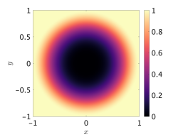
(a) $\sigma_{s}(\mathbf{x})$

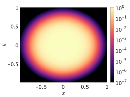
(b) Reference

Figure 2: Material cross-section and the reference scalar density $\rho$ at the final time $T=0.01$ computed using a high-order full-grid scheme for the variable scattering cross-section example.

The setup for this problem is a spatial domain given by $[-1,1]^{2}$, and we use an $S_{64}$ quadrature rule on $\mathbb{S}^{2}$. Initially, the distribution is isotropic, so we set

$$\rho(x,y,0)=\frac{1}{4\pi\zeta^{2}}\exp\left(-\frac{x^{2}+y^{2}}{4\zeta^{2}}\right),\quad g(x,y,\theta,\mu,0)=0.$$

The final time used for the simulation was $T=0.01$, and we set the time step as

$$\Delta t=0.1\epsilon\Delta x:=0.001\Delta x.$$

A plot of the material cross-section (32) as well as a plot of the high-order reference scalar density $\rho$ is shown in Fig. 2. From equation (11), we can see that the term $\sigma_{s}/\epsilon^{2}$ varies significantly across the domain and spans both the collisional and free-streaming regimes. The reference solution was obtained using a $128\times 128$ spatial mesh and an $S_{64}$ angular discretization. The particles gradually expand outward from the center of the domain and transition from a free-streaming regime to one that is strongly collisional.

Figure 3 compares the density obtained with the proposed low-rank methods against the full-grid reference density $\rho$ presented in Fig. 2b. The same $128\times 128$ spatial mesh and $S_{64}$ angular discretization was used in both of the low-rank approaches. Each plot shows the point-wise absolute difference on a logarithmic scale against a full-grid reference solution, and we use the same limits on the plots to permit a more direct comparison. It is clear that the unsplit method produces a more accurate solution than the split approach. In both cases, the most significant errors are concentrated near the center of the domain, which is where the density is the largest. When compared to the unsplit approach, we find that the errors in the split extend outward to the boundaries.

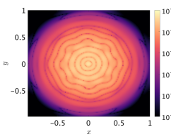
(a) High-order unsplit

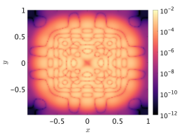
(b) High-order split

Figure 3: Point-wise absolute differences between the densities obtained with low-rank methods for the variable scattering cross-section example.

Figure 4 compares the structure of the relative singular values associated with the matricizations at each of the nodes in the dimension trees for both the unsplit and split representations. Both results were obtained using a $128\times 128$ spatial mesh and an $S_{64}$ angular discretization. The hierarchical rank of $g$ recorded at the final step was $[1,88,88,23,8]$ for the unsplit case and $[1,87,87,16,16,23,9]$ for the split case. In each of the plot windows, the vertical axis represents the relative singular values ranging from $10^{-4}$ to $1$, and the ticks correspond to logarithmic spacing in one order of magnitude. The horizontal axis uses linear spacing of the ranks from $1$ to $90$ in increments of $10$. Since this problem is restricted to the $xy-$plane, we expect symmetries to be present in the dimension $\mu$, which represents the cosine of the polar angle (dimension 3 in Fig. 4a and dimension 4 in Fig. 4b, respectively). Both methods capture this feature, as the singular values decay rapidly beyond a rank of $9$. This suggests a benefit to the tensorized angular discretization in the low-rank method. In the split approach, we note that the relative singular values of $g$ associated with the bases at the leaf nodes $\{x\}$ and $\{y\}$ (dimensions 1 and 2, respectively, in Fig. 4b) decay rapidly beyond rank 16.

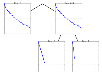
(a) Unsplit $g$

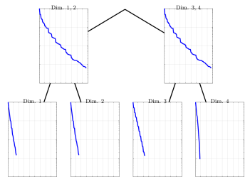
(b) Split $g$

Figure 4: Plots of the relative singular values versus rank for the matricizations at each of the nodes in the dimension tree for $g$ at the final time $T=0.01$ using unsplit and split dimension trees in the variable scattering cross-section example.

.

The time evolution of the hierarchical ranks for the tensors used to represent the microscopic component $g$ are shown in Fig. 5. We compare the unsplit and split representations using three different spatial meshes whose sizes are $32\times 32$, $64\times 64$, and $128\times 128$. While there are similarities in the growth patterns of the dimensions, both the unsplit and split approaches show a slight decrease in the hierarchical ranks for nodes associated with the spatial dimensions as the mesh resolution increases. This suggests that low-rank structures become increasingly prevalent in proportion to the mesh resolution. In both approaches, the ranks for nodes $\{x,y\}$ and $\{\theta,\mu\}$ grow the fastest, while those associated with the singleton dimensions $\{\theta\}$ and $\{\mu\}$ grow slowly with time and remain relatively small throughout the simulation. The rank of the singleton node $\{\mu\}$ remains small in each case due to the symmetry in that direction, which shows the benefit of the tensorized low-rank discretization. In problems with free-streaming and collisional features, it is worth pointing out that resolving the free-streaming component requires many ordinates, while regions of high collisionality reguire much less. The ability to use a tensorized angular domain in problems with low-rank structures means that many ordinates can be used with only a slight increase in memory cost. Similar conclusions were found in other low-rank methods, e.g., [43], where it was shown that ray effects could be eliminated by adopting more accurate angular discretizations at a slight cost in total memory. Aspects concerning the mitigation of ray-effects in kinetic problems with the proposed high-order methods is something we plan to explore in the future.

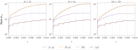
(a) High-order unsplit

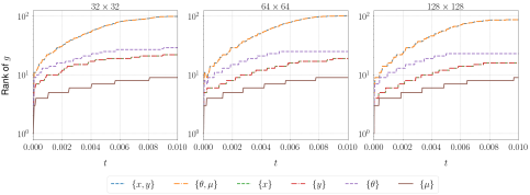
(b) High-order split

Figure 5: Time evolution of hierarchical ranks in the variable scattering cross-section example with an unsplit and split representations of the tensor $g$.

Plots showing the total DOF and the compression ratio defined by equation (6) for the proposed low-rank methods are provided in Fig. 6. We observe excellent compression ratios among both methods relative to the full-grid approach. In the unsplit approach, the compression ratio for different meshes is similar, since a full-grid representation is used in the spatial dimensions. For the split approach, the compression significantly improves as the mesh is refined, a characteristic that reflects both the curse-of-dimensionality for the full-grid solution and the low-rank structure of the numerical solution. In the case with $N=128$, we can see that the unsplit low-rank approach uses $\approx 1.09\%$ of the storage for the full-grid approach. The improvements are far more significant for the split approach, which uses $\approx 0.04\%$ of the storage for the full-grid solution. This difference in the compression results from a reduction in the total DOF by a factor of $\approx 26.48$ in the split approach versus the analogous unsplit approach, at the cost of an increase in error. The use of projections produces a comparable number of total DOF, irrespective of the resolution, when compared against the same method without the projection. This indicates that the use of the projections for conservation of macroscopic variables does not increase the total DOF and the memory complexity in a significant way.

Lastly, we include plots to confirm the conservation properties of the proposed low-rank methods in Fig. 7. When the projection for $g$ is not used, the total mass for $g$ grows to a size which is $\mathcal{O}(1)$, which improves, only slightly, as the mesh is refined. The projection ensures that the total mass contributed by $g$ remains small throughout the simulation. In terms of overall mass conservation, we find both the split and unsplit approaches are effective. We remark that the unsplit approach does not apply truncation to $\rho$, so the total mass is conserved on the order of machine precision, so we do not show this result. The split approach, which applies truncation to $\rho$, shows more noticeable violations in total mass conservation, if the projection for $\rho$ discussed in Section 3.5.1 is not used.

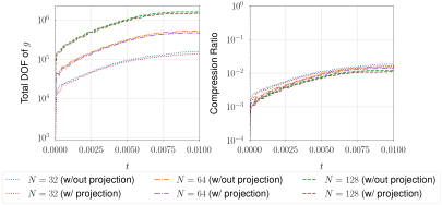
(a) High-order unsplit

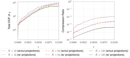
(b) High-order split

Figure 6: Plots of the total DOF and compression ratio as functions of time for the variable scattering cross-section example.

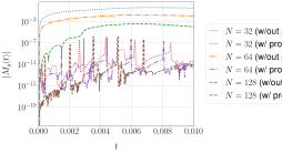
(a) High-order unsplit

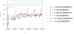
(b) High-order split

Figure 7: Absolute mass of the microscopic component $g$ for the variable scattering cross-section example.

4.3 Lattice Problem

The next example we consider is a modification of the lattice problem [4, 5], which is used as a model of a simplified fuel rod assembly in a nuclear reactor. The spatial domain for this problem is the square $[0,7]^{2}$ which is divided into smaller squares of unit area. A source is placed in the center of the domain and absorbing regions are placed around it in a configuration that resembles a checkerboard. The remaining parts of the domain are treated as purely scattering regions. This is regarded as a challenging example due to the discontinuities featured in the material data, which abruptly alternate between optically thin and thick. While it is more conventional to use outflow boundary conditions, is it also possible to adopt periodic boundary conditions, which is the approach taken here.

The profiles of the absorption and scattering cross-sections, along with the source function, are provided in Fig. 8. We initialize the macroscopic and microscopic variables as

$$\rho(x,y,0)=\frac{1}{4\pi\zeta^{2}}\exp\left(-\frac{\left(x-3.5\right)^{2}+\left(y-3.5\right)^{2}}{4\zeta^{2}}\right),\quad g(x,y,\theta,\mu,0)=0,$$

and take $\zeta=0.1$. We test the method in the kinetic regime by taking the Knudsen number $\epsilon=1$. The angular domain is discretized using an $S_{64}$ angular quadrature rule on $\mathbb{S}^{2}$. We run the simulation to a final time of $T=2.0$ and set the time step as

$$\Delta t=0.1\Delta x.$$

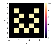
(a) $\sigma_{a}(\mathbf{x})$

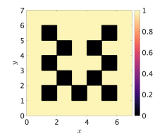
(b) $\sigma_{s}(\mathbf{x})$

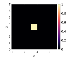
(c) $Q(\mathbf{x})$

Figure 8: Material data used in the lattice example.

We consider the impact of a low-order scheme on low-rank structures by comparing against the high-order scheme adopted in this work. Low-order discretizations are known to be more dissipative than high-order methods, which is an important consideration in the development of low-rank methods, as it can lead to the introduction of artificial low-rank structures. Two different pairings of discretizations for time and space are considered. The high-order schemes use the time and space discretizations discussed at the beginning of Section 4. For the low-order discretization, we combine the first-order IMEX method with a second-order, slope-limited, piecewise linear reconstruction method for space. Limiting in the low-order approach was performed using the MUSCL limiter [46]. Sample plots of the density $\rho$ obtained with different low-rank methods obtained with a $128\times 128$ spatial mesh and $S_{64}$ angular discretization are shown in Fig. 9 and Fig. 10. The former shows contour plots of the densities, while the latter shows $x$ and $y$ cross-sections of the densities. We note that negative values for the density are observed in the vicinity of the absorbing regions where the density is small. In the contour plots, which use logarithmic scales, we replace the negative values with $10^{-40}$. While this does not impact the stability of the method, such features more noticeable in the split approach. As expected, excessive dissipation is observed in the low-rank scheme based on the low-order discretization.

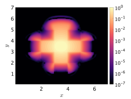
(a) High-order unsplit

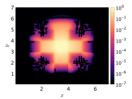
(b) High-order split

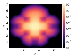
(c) Low-order unsplit

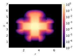
(d) Reference

Figure 9: The scalar density $\rho$ at the final time $T=2.0$ obtained with different low-rank methods for the lattice problem. We include the high-order reference solution for comparison.

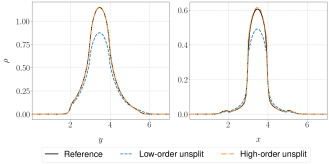
Figure 10: A comparison of unsplit low-rank methods constructed with low-order and high-order discretizations for time and space applied to the lattice problem. We show slices of the scalar density at time $T=2.0$ along the lines $x=3.5$ (left column) and $y=4.046875$ (right column).

In Fig. 11, we show plots of the point-wise absolute differences between the densities obtained with the different low-rank methods. In each case, we use the same $128\times 128$ spatial mesh with an identical $S_{64}$ angular discretization and compare the solution against the full-grid implementation. As with the previous example, we find that the high-order unsplit approach yields a better overall approximation of the full-grid solution than the corresponding split approach. Again, we find that the most significant errors are concentrated near the source, which is placed at the center of the domain. In particular, we observe more significant errors at points that coincide with the discontinuities present in the material cross-sections $\sigma_{a}$ and $\sigma_{s}$. The low-rank scheme based on the low-order discretization shows considerably larger errors in these regions due to excessive dissipation. Additionally, we observe significant smearing of the density at the corners where the material abruptly changes from optically thin to thick. Such features are better preserved with the high-order discretizations.

(a) High-order unsplit

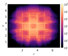
(b) High-order split

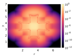
(c) Low-order unsplit

Figure 11: Point-wise absolute differences between the densities obtained with a full-grid method and low-rank methods for the lattice problem.

Figure 12 shows the structure of the relative singular values for the matricizations at each of the nodes in the dimension tree for $g$ obtained with unsplit and split approaches using high-order discretizations. These results were obtained using a $128\times 128$ spatial mesh and an $S_{64}$ angular discretization. The hierarchical rank of $g$ recorded at the final step was $[1,357,357,61,13]$ for the unsplit case and $[1,358,358,46,47,58,14]$ for the split case. In each of the plot windows, the vertical axis represents the relative singular values ranging from $10^{-4}$ to $1$, and the ticks correspond to logarithmic spacing in one order of magnitude. The horizontal axis uses linear spacing of the ranks from $1$ to $360$ in increments of $10$. We note that both methods show high rank in the nodes $\{x,y\}$ and $\{\theta,\mu\}$. Further, the split approach shows a reasonable decay along the dimensions associated with individual spatial dimensions (e.g., dimensions 1 and 2 in Fig. 12b). Additionally, we expect the solution $g$ to exhibit a stronger angular dependence given that this problem is more kinetic than the previous example. Further, the presence of jump discontinuities in the material data places a significant demand on the global basis of the tensor method. However, we still find tensorization of the angular domain to be beneficial for this problem, as the singular values associated with the dimensions $\{\theta\}$ and $\{\mu\}$ (dimensions 2 and 3 in Fig. 12a and dimensions 3 and 4 in Fig. 12b, respectively) show reasonable decay that, again, reflects the symmetry in $\mu$.

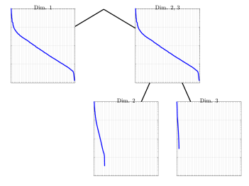
(a) High-order unsplit

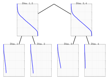
(b) High-order split

Figure 12: Plots of the relative singular values versus the rank for the matricizations at each of the nodes in the dimension tree for $g$ at the final time $T=2$ using unsplit (left) and split (right) dimension trees in the lattice problem.

The time evolution of the hierarchical ranks of $g$ with unsplit and split high-order discretizations are presented in Fig. 13. We, again, considered three different spatial meshes whose sizes are $32\times 32$, $64\times 64$, and $128\times 128$. Unlike the previous example, we find that the maximum rank of $g$ increases with the resolution of the mesh across each of the dimensions. For both the unsplit and split dimension trees, we, again, find that the nodes associated with $\{x,y\}$ and $\{\theta,\mu\}$ grow significantly faster than those associated with the angular dimensions, a feature that persists for each of the simulations. We also find that the rank growth for the angular dimensions follows similar patterns in both the unsplit and split approaches. The hierarchical ranks associated with the nodes $\{x\}$ and $\{y\}$, in the split approach, indicate the presence of low-rank features that can reduce the total DOF. Unlike the previous example, the maximum hierarchical rank for this problem is seen to increase with the mesh resolution, as the grid begins to resolve fine-scale features. This is observed regardless of the dimension tree. The growth of the hierarchical ranks in the high-dimensional function $g$ obtained using the low-order approach is provided in Fig. 14. The low-order scheme shows no growth in the hierarchical ranks of $g$ after time $t\approx 1.5$. Comparing this with Fig. 13a, which corresponds to the high-order scheme, shows several key differences. Most notably, the latter shows growth in the ranks until the final time of the simulation. Additionally, the overall size of the ranks obtained with the low-order approach are considerably smaller than those obtained with the high-order method. For example, at the final time of the simulation using the $128\times 128$ mesh, the hierarchical ranks of g are $[1,132,132,35,8]$ and $[1,357,357,61,13]$ for the low-order and high-order approaches, respectively. This indicates that additional ranks are necessary in order to achieve a more faithful representation of the function $g$. A closer examination of the data collected at the final time for this case reveals that the high-order method uses a factor of $\approx 2.82$ times more total DOF of than the low-order scheme. However, the additional DOF is more than compensated by the increase in accuracy, as indicated in Figure 11.

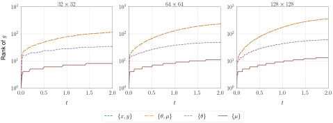
(a) High-order unsplit

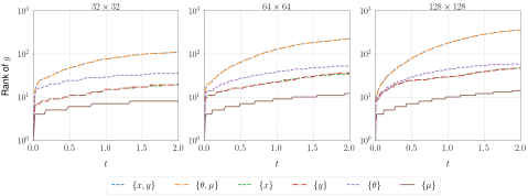
(b) High-order split

Figure 13: Time evolution of hierarchical ranks in the lattice problem using unsplit (top row) and split (bottom row) representations of the tensor $g$.

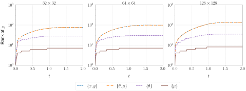
Figure 14: Time evolution of hierarchical ranks in the lattice problem obtained with an unsplit low-rank scheme based on low-order discretizations for time and space.

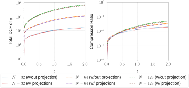
(a) High-order unsplit

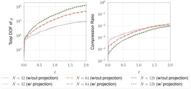
(b) High-order split

Figure 15: Plots of the total DOF and compression ratio as functions of time for the lattice problem.

The growth in the total DOF and compression ratio for the low-rank methods is presented in Figure 15. Despite the growth in the rank, we find that the low-rank methods still offer reasonable compression of the function $g$. For example, we find that unsplit low-rank method requires $\approx 4.67\%$ of the storage needed for the full-grid representation when a $128\times 128$ spatial mesh is used with an $S_{64}$ angular discretization. The same case, using the split approach, yields a compression ratio of $\approx 0.90\%$. As with the previous example, we find that the use of the projection technique does not have significant memory overhead in terms of the total DOF for the function $g$. Note that the unsplit method produces worse compression compared to the split method as the mesh resolution increases.

5 Conclusions

This work contributed novel low-rank approximation techniques for the solution of the multi-scale linear kinetic transport equation. The approach we take utilizes a macro-micro decomposition of the distribution function to ensure that the scheme recovers the linear diffusion equation in the appropriate asymptotic limits. The proposed low-rank methods support rank adaptivity and address challenges intrinsic to the curse of dimensionality through the use of the HTT format. The new methods, which eliminate the projector-splitting used by existing low-rank methods, offer enhanced flexibility in coupling low-rank methods with high-order discretizations for both time and space. We presented a variety of numerical results to demonstrate the capabilities of the proposed methods. A key benefit of the proposed methods is the significant reduction in the storage costs relative to a full-grid implementation. We also demonstrated the impact of accuracy of the discretization on the low-rank structures, which indicates that great care should be taken when choosing discretizations. We are currently combining the proposed framework with discontinuous Galerkin discretizations to accommodate more general boundary conditions in transport applications. Additionally, we are planning to extend the methods presented in this work to the implicit setting, which will further reduce the stiffness near the diffusion limit.

References

- [1] U. M. Ascher, S. J. Ruuth, and R. J. Spiteri, Implicit-explicit Runge-Kutta methods for time-dependent partial differential equations, Applied Numerical Mathematics, 25 (1997), pp. 151–167.
- [2] Y. Azmy, E. Sartori, E. W. Larsen, and J. E. Morel, Advances in discrete-ordinates methodology, Nuclear computational science: A century in review, (2010), pp. 1–84.
- [3] S. Boscarino, L. Pareschi, and G. Russo, Implicit-explicit Runge–Kutta schemes for hyperbolic systems and kinetic equations in the diffusion limit, SIAM Journal on Scientific Computing, 35 (2013), pp. A22–A51.
- [4] T. A. Brunner, Forms of approximate radiation transport, Tech. Report SAND2002-1778, Sandia National Lab.(SNL-NM), Albuquerque, NM (United States), 2002.
- [5] T. A. Brunner and J. P. Holloway, Two-dimensional time dependent Riemann solvers for neutron transport, Journal of Computational Physics, 210 (2005), pp. 386–399.
- [6] G. Ceruti, J. Kusch, and C. Lubich, A rank-adaptive robust integrator for dynamical low-rank approximation, BIT Numerical Mathematics, 62 (2022), pp. 1149–1174.
- [7] G. Ceruti and C. Lubich, An unconventional robust integrator for dynamical low-rank approximation, BIT Numerical Mathematics, 62 (2022), pp. 23–44.
- [8] J. Coughlin, J. Hu, and U. Shumlak, Robust and conservative dynamical low-rank methods for the Vlasov equation via a novel macro-micro decomposition, Journal of Computational Physics, 509 (2024), p. 113055.
- [9] G. Dimarco and L. Pareschi, Asymptotic preserving implicit-explicit runge–kutta methods for nonlinear kinetic equations, SIAM Journal on Numerical Analysis, 51 (2013), pp. 1064–1087.
- [10] G. Dimarco, L. Pareschi, and G. Samaey, Asymptotic-preserving monte carlo methods for transport equations in the diffusive limit, SIAM Journal on Scientific Computing, 40 (2018), pp. A504–A528.
- [11] Z. Ding, L. Einkemmer, and Q. Li, Dynamical low-rank integrator for the linear Boltzmann equation: error analysis in the diffusion limit, SIAM Journal on Numerical Analysis, 59 (2021), pp. 2254–2285.
- [12] L. Einkemmer, Accelerating the simulation of kinetic shear Alfvén waves with a dynamical low-rank approximation, Journal of Computational Physics, 501 (2024), p. 112757.
- [13] L. Einkemmer, J. Hu, and J. Kusch, Asymptotic-preserving and energy stable dynamical low-rank approximation, SIAM Journal on Numerical Analysis, 62 (2024), pp. 73–92.
- [14] L. Einkemmer, J. Hu, and Y. Wang, An asymptotic-preserving dynamical low-rank method for the multi-scale multi-dimensional linear transport equation, Journal of Computational Physics, 439 (2021), p. 110353.
- [15] L. Einkemmer, J. Hu, and L. Ying, An efficient dynamical low-rank algorithm for the Boltzmann-BGK equation close to the compressible viscous flow regime, SIAM Journal on Scientific Computing, 43 (2021), p. 1057–B1080.
- [16] L. Einkemmer and I. Joseph, A mass, momentum, and energy conservative dynamical low-rank scheme for the Vlasov equation, Journal of Computational Physics, 443 (2021), p. 110495.
- [17] L. Einkemmer and C. Lubich, A low-rank projector-splitting integrator for the Vlasov–Poisson equation, SIAM Journal on Scientific Computing, 40 (2018), pp. B1330–B1360.
- [18] M. Frank, C. Hauck, and K. Küpper, Convergence of filtered spherical harmonic equations for radiation transport, Communications in Mathematical Sciences, 14 (2016), pp. 1443–1465.
- [19] L. Grasedyck, Hierarchical singular value decomposition of tensors, SIAM Journal on Matrix Analysis and Applications, 31 (2010), p. 2029–2054.
- [20] K. Grella and C. Schwab, Sparse discrete ordinates method in radiative transfer, Computational Methods in Applied Mathematics, 11 (2011), pp. 305–326.
- [21] W. Guo and Y. Cheng, A sparse-grid discontinuous Galerkin method for high-dimensional transport equations and its application to kinetic simulations, SIAM Journal on Scientific Computing, 38 (2016), pp. A3381–A3409.
- [22] W. Guo and Y. Cheng, An adaptive multiresolution discontinuous Galerkin method for time-dependent transport equations in multidimensions, SIAM Journal on Scientific Computing, 39 (2017), pp. A2962–A2992.
- [23] W. Guo, J. F. Ema, and J.-M. Qiu, A local macroscopic conservative (LoMaC) low rank tensor method with the discontinuous Galerkin method for the Vlasov dynamics, Communications on Applied Mathematics and Computation, (2023).
- [24] W. Guo and J.-M. Qiu, A low rank tensor representation of linear transport and nonlinear Vlasov solutions and their associated flow maps, Journal of Computational Physics, 458 (2022), p. 111089.
- [25] W. Guo and J.-M. Qiu, A conservative low rank tensor method for the Vlasov dynamics, SIAM Journal on Scientific Computing, 46 (2024), pp. A232–A263.
- [26] W. Hackbusch and S. Kühn, A new scheme for the tensor representation, Journal of Fourier Analysis and Applications, 15 (2009), pp. 706–722.
- [27] C. D. Hauck and S. Schnake, A predictor-corrector strategy for adaptivity in dynamical low-rank approximations, SIAM Journal on Matrix Analysis and Applications, 44 (2023), pp. 971–1005.
- [28] J. Hu and Y. Wang, An adaptive dynamical low rank method for the nonlinear Boltzmann equation, Journal of Scientific Computing, 92 (2022), p. 75.
- [29] J. Jang, F. Li, J.-M. Qiu, and T. Xiong, High order asymptotic preserving DG-IMEX schemes for discrete-velocity kinetic equations in a diffusive scaling, Journal of Computational Physics, 281 (2015), pp. 199–224.
- [30] K. Kormann, A semi-Lagrangian Vlasov solver in tensor train format, SIAM Journal on Scientific Computing, 37 (2015), pp. B613–B632.
- [31] D. Kressner and C. Tobler, htucker—a MATLAB toolbox for tensors in hierarchical Tucker format, Mathicse, EPF Lausanne, (2012).
- [32] J. Krotz, C. D. Hauck, and R. G. McClarren, A hybrid Monte Carlo, discontinuous Galerkin method for linear kinetic transport equations, 2023, https://arxiv.org/abs/2312.04217.
- [33] L. D. Lathauwer, B. D. Moor, and J. Vandewalle, A multilinear singular value decomposition, SIAM Journal on Matrix Analysis and Applications, 21 (2000).
- [34] V. Lebedev, Quadratures on a sphere, USSR Computational Mathematics and Mathematical Physics, 16 (1976), pp. 10–24.
- [35] M. Lemou and L. Mieussens, A new asymptotic preserving scheme based on micro-macro formulation for linear kinetic equations in the diffusion limit, SIAM Journal on Scientific Computing, 31 (2008), pp. 334–368.
- [36] C. Lubich and I. V. Oseledets, A projector-splitting integrator for dynamical low-rank approximation, BIT Numerical Mathematics, 54 (2014), pp. 171–188.
- [37] R. G. McClarren and C. D. Hauck, Robust and accurate filtered spherical harmonics expansions for radiative transfer, Journal of Computational Physics, 229 (2010), pp. 5597–5614.
- [38] R. G. McClarren, J. P. Holloway, and T. A. Brunner, On solutions to the equations for thermal radiative transfer, Journal of Computational Physics, 227 (2008), pp. 2864–2885.
- [39] W. F. Miller and E. E. Lewis, Computational methods of neutron transport, Wiley, 1993.
- [40] I. Oseledets, Tensor-train decomposition, SIAM Journal on Scientific Computing, 33 (2011), p. 295–2317.
- [41] Z. Peng, Y. Chen, Y. Cheng, and F. Li, A micro-macro decomposed reduced basis method for the time-dependent radiative transfer equation, Multiscale Modeling & Simulation, 22 (2024), pp. 639–666.
- [42] Z. Peng and R. G. McClarren, A high-order/low-order (HOLO) algorithm for preserving conservation in time-dependent low-rank transport calculations, Journal of Computational Physics, 447 (2021), p. 110672.
- [43] Z. Peng and R. G. McClarren, A sweep-based low-rank method for the discrete ordinate transport equation, Journal of Computational Physics, 473 (2023), p. 111748.
- [44] Z. Peng, R. G. McClarren, and M. Frank, A low-rank method for two-dimensional time-dependent radiation transport calculations, Journal of Computational Physics, 421 (2020), p. 109735.
- [45] C.-W. Shu, High order weighted essentially nonoscillatory schemes for convection dominated problems, SIAM review, 51 (2009), pp. 82–126.
- [46] B. van Leer, Upwind and high-resolution methods for compressible flow: From donor cell to residual-distribution schemes, in 16th AIAA Computational Fluid Dynamics Conference, 2006, p. 3559.
- [47] O. N. Vassiliev, Monte Carlo methods for radiation transport, Fundamentals and Advanced Topics, (2017).
- [48] G. Zhang, H. Zhu, and T. Xiong, Asymptotic preserving and uniformly unconditionally stable finite difference schemes for kinetic transport equations, SIAM Journal on Scientific Computing, 45 (2023), pp. B697–B730.