PUREPath: A Deep Latent Variational Model for Estimating CMB Posterior over Large Angular Scales of the Sky

Abstract

We present a comprehensive neural architecture, the ${\tt PUREPath}$, which leverages a nested Probabilistic multi-modal U-Net framework, augmented by the inclusion of probabilistic ResNet blocks in the Expanding Pathway of the decoders, to estimate the posterior density of the Cosmic Microwave Background (CMB) signal conditioned on the observed CMB data and the training dataset. By seamlessly integrating Bayesian statistics and variational methods our model effectively minimizes foreground contamination in the observed CMB maps. The model is trained using foreground and noise contaminated CMB temperature maps simulated at Planck LFI and HFI frequency channels 30 - 353 GHz using publicly available Code for Anisotropies in the Microwave Background (CAMB) and Python Sky Model (PySM) packages. During training, our model transforms initial prior distribution on the model parameters to posterior distributions based on the training data. From the joint full posterior of the model parameters, during inference, a predicitve CMB posterior and summary statistics such as the predictive mean, variance etc of the cleaned CMB map is estimated. The predictive standard deviation map provides a direct and interpretable measure of uncertainty per pixel in the predicted mean CMB map. The cleaned CMB map along with the error estimates can be used for more accurate measurements of cosmological parameters and other cosmological analyses.

1 Introduction

The CMB fluctuations provide us valuable insights regarding the origin, geometry, and composition of our universe while rendering stringent constraints on cosmological parameters Aghanim et al. (2020). Several ground (Hincks et al., 2010; Li et al., 2019; Hui et al., 2018; Abazajian et al., 2022), ballon (Masi et al., 2002; Lazear et al., 2014; Gualtieri et al., 2018) and satellite (Bennett et al., 2003a; Ade et al., 2014; Allys et al., 2023; Adak et al., 2022) -based scientific missions have already observed or are at various stages of either planning or observing these fluctuations with increasingly higher sensitivities. However, strong microwave emissions from various galactic and extra-galactic astrophysical sources, the foregrounds, and inherent instrumental noise of the detectors contaminates the observed CMB signal. It is crucial for the success of any CMB mission to either disentangle or mitigate these foregrounds and detector-noise contributions to disinter the physics encoded in the CMB fluctuations.

Recent decades saw development of several foreground minimization and component separation methods which can be broadly classified into $parametric$ and $non-parametric$ approaches. $Parametric$ methods like Commander (Eriksen et al. (2008b), Eriksen et al. (2008a)), Template-fitting (Land & Magueijo (2006), Jaffe et al. (2006)) requires intricate modeling of either CMB and/or foregrounds to separate the CMB signal in the observed maps. On the contrary, $non-parametric$ methods makes minimal assumptions concerning the nature of the foregrounds, and CMB while estimating the CMB signal. Some of the prominent $non-parametric$ methods includes internal-linear-combination (ILC) (Bennett et al. (2003b), Eriksen et al. (2004), Tegmark et al. (2003), Delabrouille et al. (2009), Sudevan et al. (2017)) as well as Independent Component Analysis (ICA) method (Taylor et al. (2006), Hurier et al. (2013)), among others.

In recent years, due to remarkable achievements in the field of machine learning (ML) (Samuel, 1959) in tackling various complex real-world challenges, ML is actively pursued to solve intricate problems in the realm of Physics. The image processing capabilities of ML models especually with the use of convolutional layers, have spiked interest in the CMB community to invoke ML techniques for CMB analyses. Convolutional neural networks are developed to extract the CMB signal by minimizing the foregrounds in the CMB data (Petroff et al., 2020; Wang et al., 2022; Casas et al., 2022; Yan et al., 2023a, 2024), to inpaint masked regions in CMB maps (Yi et al., 2020; Montefalcone et al., 2021), delensing in CMB polarization maps (Yan et al., 2023b). ML models are also used to recognize different foreground models (Farsian et al., 2020), to remove E-B leakage in partial-sky (Pal & Saha, 2023), estimation of B-mode signal at large angular scales after removing the foregrounds (Pal et al., 2024). Adams et al. (2023) and Petroff et al. (2020) developed DeepShere (Defferrard et al., 2020) based U-Net (Ronneberger et al., 2015) with concrete dropout (Gal et al., 2017) to minimize foreground contaminations in CMB data. Concrete dropout can be used to estimate a network’s epistemic uncertainty due to insufficient training. These are some of the many instances where ML models are leveraged within CMB analyses.

In conventional ML framework, a model is trained to understand the relationship between the inputs and outputs by fixing the model parameters (${\omega}$), the weights and biases. In a deterministic neural network, these parameters remain unchanged when the network is used for predictions. They do not inherently take into account for either the epistemic or aleotoric (due to intrinsic errors in the data) uncertainty and often leads to situations where a trained network makes overly confident predictions on new unseen data.

Probabilistic neural networks (Specht, 1990) like Bayesian neural networks are developed to address this crucial shortcoming of the standard deep neural networks by incorporating uncertainty considerations in both the model and the data. Bayesian networks utilizes probabilistic layers in order to capture the uncertainty over weights or activations or both by incorporating prior knowledge of the parameters and propagating it through the network, thereby modeling the uncertainty in the predictions. This is achieved through Bayesian inference (Tipping, 2004), where the posterior distribution over model parameters is updated given the training data by using Bayes’ theorem. Since Bayesian posteriors are usually intractable, variational inference (VI) techniques like variational Bayes (Kingma & Welling (2013), Hoffman et al. (2013)) and stochastic gradient variational Bayes (Knowles (2015)) are developed. These methods approximate the posterior distribution of the model parameters by optimizing a tractable surrogate distribution. Probabilistic layers in Bayesian networks provide a more intuitive way to understand the uncertainty associated with the model and its predictions. However, constructing and training a fully Bayesian neural network can be challenging and is nontrivial even in relatively simple applications.

Our ${\tt PUREPath}$ is designed to minimize foreground contaminations in the observed full-sky CMB maps. The full-sky maps are projected into a plane and divided into $n_{\tt reg}$ distinct and disjoint regions as shown in Figure 1 during pre-processing. ${\tt PUREPath}$ architecture is best characterised as a probabilistic, nested framework composed of $n_{\tt reg}$ probabilistic U-Net. Each U-Net consists of $n_{\tt map}$ encoders to facilitate a multi-modal learning, a latent space, and a decoder with probabilistic ResNets (He et al., 2015) in the expanding pathway of each decoders at skip connections. The output of our model is a distribution defined by MultivariateNormalDiag layer with inputs, the mean and scale$\_$diag, as the decoder outputs. More details regarding our model is provided in Section 3.

2 Formalism

We briefly review how a Bayesian neural network which utilizes probabilistic layers is trained using Variational Inference.

2.1 Bayesian Neural Network

The parameters (${\omega}$) in a Bayesian network are stochastic in nature and are sampled from respective posterior distributions $P(\omega|\mathcal{D})$. Here, $\mathcal{D}$ is the training dataset with inputs $\Bigl{\{}{\bf X}_{j}=\{{\bf x}_{i,\,j}\}_{i=1}^{n}\Bigl{\}}_{j=1}^{N}$, comprising of $N$ simulated sets of foreground contaminated CMB maps ${\bf x}_{i}$ at $n$ frequencies, and $N$ output ${\bf y}_{j}$ (the input simulated CMB map for the set $j$) i.e.,

$$\mathcal{D}=\Bigl{\{}\{{\bf x}_{i,\,j}\}_{i=1}^{n},{\bf y}_{j}\Bigl{\}}_{j=1}^{N}$$ (1)

In the Bayesian approach, a prior distribution $P({\omega})$ of the model parameters $\omega$ is assumed based on the assumption as to which functions best generates the data. For a given $P({\omega})$ and $\mathcal{D}$, the posterior distribution $P(\omega|\mathcal{D})$ (Graves (2011)) is updated using the Bayes’ principle as follows:

$$P(\omega|\mathcal{D})=\frac{P(\mathcal{D}|\omega)P({\omega})}{P(\mathcal{D})}\,.$$ (2)

$P(\mathcal{D}|\omega)=\Pi_{i=1}^{N}P({\bf y}_{i}|{\bf X}_{i},\omega)$ is $likelihood$ of the observing ${\bf y}_{i}$ given ${\bf X}_{i}$ and set of model parameters $\omega$.

Accurate estimation of exact $P(\omega|\mathcal{D})$ using Bayesian inference is not practical as it requires integrating over all feasible values of $\omega$. A simpler alternative is to approximate the exact distribution with a more tractable surrogate or variational distribution $Q_{\theta}({\omega})$ with parameters $\theta$, the VI technique. These variational parameters ($\theta$) are optimized to minimize the difference between approximate and true posteriors. In practice, we minimize the the Kullback-Leibler (KL) divergence $\mathbb{D}_{KL}(Q_{\theta}({\omega})||P({\omega}|\mathcal{D}))$ (Kullback & Leibler, 1951),

$$\mathbb{D}_{KL}(Q_{\theta}({\omega})||P({\omega}|\mathcal{D}))=\mathbb{E}_{Q}[\log Q_{\theta}({\omega})]-\mathbb{E}_{Q}[\log P({\omega}|\mathcal{D})]+\log(P(\mathcal{D}))\,.$$ (3)

to find these variational parameters. The goal of optimization procedure is to determine the $\theta$ which minimizes KL-divergence, thereby facilitating a more practical approximation of the true posterior. During implementation, the usual approach is to maximize the so-called evidence lower bound (ELBO) (David M. Blei & McAuliffe, 2017),

$$ELBO(Q) =\mathbb{E}_{Q}[\log P({\mathcal{D}}|\omega)]-\beta D_{KL}(Q_{\theta}(\omega)||P(\omega|{\mathcal{D}}))\,.$$ (4)

Here, $\mathbb{E}_{Q}[\log P({\mathcal{D}}|\omega)]$ is the expected log-likelihood under the variational distribution $Q_{\theta}({\omega})$. $\beta$ is a tunable hper parameter to weight the KL-Diveregence. ELBO is preferred to train Bayesian networks as it serves as a lower bound on the log marginal likelihood of the data and also measures the quality of the approximate posterior. The loss function ($\mathbb{L}$) is defined as the negative of ELBO,

$$\mathbb{L}_{\tt ELBO}=-ELBO(Q)\,.$$ (5)

During the training phase, this loss is minimized to find the optimal values of $\theta$ that defines the parameters of the distribution over weights. The distribution $Q_{\theta}(\omega)$ can be described in terms of weight perturbations $\omega=\bar{\omega}+\Delta\omega$, where $\bar{\omega}$ and $\Delta\omega$ are the mean weights and a stochastic perturbation for ${\omega}$ respectively, $\theta=\{\bar{\omega},\Delta\omega\}$.

Figure 1: In the left panel we show a simulated CMB map using HealPix Mollewide projection. The map is divided with solid black lines into 12 equal area regions. These 12 regions are of dimension $N_{\tt side}\,\times\,N_{\tt side}$ and are stitched together to form the four plane images of dimension $N_{\tt side}\,\times\,3N_{\tt side}$. The choice of the regions in the planar maps is such that the regions which are in contact in the planar maps are also in contact in the real sky and the dimension of all images is same.

2.2 Weight Perturbations with Flipout

We follow a weight perturbation technique known as the Flipout (Wen et al., 2018) to train our network. This method is based on two key assumptions regarding the nature of perturbations $\Delta\omega$, the perturbations of different weights are independent to each other and their distribution is symmetric around zero. Under these assumptions, the distribution of the perturbations is invariant to an element-wise multiplication by a random sign matrix. Flipout introduces a common base perturbation $\Delta\hat{\omega}$ during training, which is shared by all training examples in a mini-batch. For each individual example, the corresponding weight perturbations are achieved as follows:

$$\Delta\omega=\Delta\hat{\omega}\circ r_{n}s_{n}^{T}\,.$$ (6)

Here, the subscript $n$ denotes the index of the data-points in a mini-batch. $r_{n}$ and $s_{n}$ are entries of random vectors uniformly sampled from $\pm 1$. Flipout technique introduces different weight perturbations for each example in a mini-batch thus ensuring the gradients to be decorrelated between different training examples in a mini-batch. This significantly reduce the variance in the gradient updates when averaging over a mini-batch.

For Bayesian networks, $\bar{\omega}$ and $\Delta\hat{\omega}$ are obtained via standard backpropogation with stochastic optimization algorithms. For mini-batch optimization, the batch loss is written as

$$\mathbb{L}_{i}=\beta D_{KL}(Q_{\theta}({\omega})||P(\theta))-\frac{1}{N}\sum_{n=1}^{N}\log P({\mathcal{D}}_{i}^{n}|{\bf\omega}^{i})\,,$$ (7)

where $i$ iterates over the mini-batch indices, $n$ and $N$ represents the index corresponding to the particular example in the mini-batch and total size of each mini-batch respectively. Even though only one set of parameters ${\omega}^{i}$ is drawn from $Q_{\theta}({\omega})$ for each mini-batch, Flipout ensures the parameters are different for each individual examples ${\mathcal{D}}_{i}^{n}$.

2.3 Estimating CMB Posterior

After training, the model provides a variational posterior $Q_{\theta}({\omega|\theta^{\ast}})$, where $\theta^{\ast}$ are the optimized values of the parameters of the variational distribution. The predictive CMB posterior ${\hat{P}}({\bf y}^{\ast}|{\bf X}^{\ast},\mathcal{D})$ of the estimated cleaned CMB map (${\bf y}^{\ast}$) conditioned on the input maps (${\bf X}^{\ast}$) and the training dataset ($\mathcal{D}$), is estimated using the variational posterior $Q_{\theta}({\omega|\theta^{\ast}})$ of the model parameters as follows,

$${\hat{P}}({\bf y}^{\ast}|{\bf X}^{\ast},\mathcal{D}) =\int{\hat{P}}({\bf y}^{\ast}|{\bf X}^{\ast},\omega)P(\omega|\mathcal{D})d\omega$$

$$\approx\int{\hat{P}}({\bf y}^{\ast}|{\bf X}^{\ast},\omega)\mathcal{Q}_{\theta}(\omega|\theta^{\ast})d\omega\,.$$ (8)

This integral can be numerically evaluated using Monte Carlo (MC) sampling as:

$${\hat{P}}({\bf y}^{\ast}|{\bf X}^{\ast},\mathcal{D})\approx\frac{1}{S}\sum_{s=1}^{S}{\hat{P}}({\bf y}^{\ast}|{\bf X}^{\ast},\omega^{s})\,,$$ (9)

where, ${\hat{P}}({\bf y}^{\ast}|{\bf X}^{\ast},\omega^{s})$ is a predictive distribution corresponding to the model parameters $\omega^{s}$ sampled from $Q_{\theta}({\omega|\theta^{\ast}})$ i.e., $\omega^{s}\,\sim\,Q_{\theta}({\omega|\theta^{\ast}}$). $s$ and $S$ in Eqn. 9 represents the index of the sampling step and the total number of MC samplings respectively. ${\hat{P}}({\bf y}^{\ast}|{\bf x}^{\ast},\omega^{s})=\mathcal{N}({\bf y}^{\ast}|\mu_{\tt CMB}({\bf x}^{\ast},\omega^{s}),\sigma_{\tt CMB}({\bf x}^{\ast},\omega^{s}))$ (Abdar et al., 2021) where $\mu_{\tt CMB}$ and $\Sigma_{\tt CMB}$ are the predictive mean and variance estimated from the samples generated in the step $s$.

2.4 Estimation of Uncertainty

The advantage of implementing a Bayesian network is its ability to quantify both epistemic and aleatoric uncertainty. From the predictive CMB posterior distribution ${\hat{P}}({\bf y}^{\ast}|{\bf x}^{\ast},\mathcal{D})$, we can compute summary statistics such as the predictive mean, variance and other higher-order statistics of the cleaned CMB map. To quantify the uncertainty in the predictions, we estimate the predictive mean, variance and standard deviation etc as follows:

$$\mathbb{E}[{\bf y}^{\ast}|{\bf x}^{\ast},{\mathcal{D}}] \approx\frac{1}{S}\sum_{s=1}^{S}\mu_{\tt CMB}^{s}\,,$$ (10)

$$Var[{\bf y}^{\ast}|{\bf x}^{\ast},\mathcal{D}] \approx\frac{1}{S}\sum_{s=1}^{S}\Bigl{(}(\mu_{CMB}^{s}-\mathbb{E}[{\bf y}^{*}])^{2}+(\sigma_{\tt CMB}^{s})^{2}\Bigl{)}\,,$$ (11)

$$\sigma[{\bf y}^{\ast}|{\bf x}^{\ast},\mathcal{D}] =\sqrt{Var[{\bf y}^{\ast}|{\bf x}^{\ast},\mathcal{D}]}\,.$$ (12)

3 Network Architecture

The ${\tt PUREPath}$’s hybrid architecture is shown in Figure 2. Depending on the total number of regions $N_{\tt reg}$ our network has that many U-Nets to process images corresponding to each regions. All the feature extraction layers in the U-Nets and ResNets are Tensorflow Probability (Abadi et al., 2015) Convlution2DFlipout layers with kernel size $3\times 5$ and strides 1 and with parametric-RELU (p-RELU) activation. They are initialized using default multivariate normal distributions with random mean and standard deviation and mean-field normal functions provided by Tensorflow as prior and posterior respectively. We perform a strided convolution to downsample the image with stride set to 2 in the Convoultion2DFlipout followed by p-ReLU activation. The number of filters for all the convolution layers in the encoder is fixed at 16. The feature maps from the final layer of all the encoders in a U-net are combined together by performing an element-wise addition along the channels axis to from a high-dimensional, abstract representation of the input images in the latent space. These represenations are passed to decoder along with the encoder outputs. The decoder consists of ResNet Block in its expanding pathway at every skip-connection. In our formulation of ResNet (refer to Figure 2) three back-to-back convolutions operations are performed each followed by an activation with p-RELU and BatchNormalization. After these operations, the input is added back to the new feature maps to form the residual connection. The three consecutive convolution operations within each ResNet block uses Convolution2DFlipout with kernel sizes $1\times 1$, $3\times 5$ and $1\times 1$. This process is repeated total 6 times. The three ResNet blocks in the decoder has input and ouput convolution filters set at (16, 16), (16, 32) and final block has (32, 32). The feature maps from the final ResNet block is sent to two Convolution2DFlipout layers with p-ReLU activation and kernel size (1,1), thereby allowing each decoder to generate two feature maps at original input image dimension at the output. The final layer of our network is a distribution defined by a ‘MultivariateNormalDiag’ layer parametrized by two inputs: ‘${\tt loc}$’ and ‘${\tt scale\_diag}$’. The inputs are obtained by concatenating corresponding feature map from all the decoders and flattening them to get arrays of length $N_{\tt pix}$, where $N_{\tt pix}$ is the total number of pixels in the full-sky map as shown in Figure 1. This layer introduces a probabilistic element to the output and the mean of the distribution is the predicted output while the standard deviation is interpreted as the model’s uncertainty in the prediction, thereby offering insights into the robustness and reliability of the model’s output.

Figure 2: A pictorial representation of our ${\tt PUREPath}$ Model. Each Region has its own multi-encoder-latent-decoder units. Each encoder block in turn has separate encoder units to process each input map in that region merging into a single latent space and finally to a single Decoder unit. All the output feature maps finally goes to a MultivariateNormalDiag layer, the output of our model.

4 Data Simulations

We train our network using foreground and noise contaminated CMB maps at several Planck frequency channels simulated using publicly available software packages CAMB (Lewis & Challinor, 2011), HealPix (Górski et al., 2005), and PySM Thorne et al. (2017). CAMB and PySM packages are employed to generate 1200 full-sky CMB simulations based on the $\Lambda$ cold dark matter framework. We sample the following cosmological parameters $H_{0}$, $\Omega_{b}$, $\Omega_{c}$, $\tau$, $A_{s}$, $n_{s}$ from their respective Gaussian distribution $\mathcal{N}(m_{P},\sigma_{P}^{2})$, with $m_{P}$ set to the best-fit value provided by Aghanim et al. (2020) and with a 1$\sigma$ standard deviation. Employing CAMB, we generate a lensed CMB power spectrum, corresponding to the sampled set of cosmological parameters, and the full-sky map with PySM.

Foreground emission maps are simulated using PySM at 7 Planck frequencies i.e., Planck LFI 30, 44, 70 GHz, and Planck HFI 100, 143, 217 and 353 GHz. The dominant sources of contaminators we consider are: thermal dust, synchrotron, free-free and anomolous microwave emission (AME). For thermal dust we use ‘d1 model’ provided by PySM, while ‘s1 model’ is employed to simulate synchrotron emissions. Free-free and AME simulations are generated using ‘f1’ and ‘a2’ model respectively. To train our network efficiently, we simulate 1200 realizations of these foregrounds at all frequencies of interest by sampling amplitude $A_{\tt foreg}$ and spectral index $\beta_{\tt foreg}$ of these foregrounds from a Gaussian distribution. The mean of this distribution is the corresponding $A_{\tt foreg}$ or $\beta_{\tt foreg}$ template provided by PySM and a standard deviation of 10$\%$ from the mean value.

To create 1200 noise realizations for the Planck LFI and HFI maps, we use the intensity noise variance values given in the fifth column of the respective frequency band Planck map files. Noise is assumed to be Gaussian, isotropic and uncorrelated between pixel to pixel. All the CMB, foregrounds and Noise maps are generated at HealPix $N_{\tt side}=32$ with a Gaussian smoothing of FWHM $1.83^{\circ}$ ($\approx$ size of pixel in a HealPix map of $N_{\tt side}=32$). We co-add 1200 samples of CMB, four different foregrounds and noise realizations corresponding to each of the 7 Planck frequency channels, to generate 1200 sets of simulated foreground contaminated CMB maps at each frequency.

4.1 Data Preprocessing

The spherical full-sky maps are transformed into approximate plane images (Wang et al., 2022) by reoredering all the maps from native HealPix Ring format to Nested pixellation scheme and then divide the resulting Nested maps into 12 equal area regions as shown in Figure 1. Each of these pieces are of dimension ($N_{\tt side}\times N_{\tt side}$). After this, we arrange three pieces together forming 4 independent ($N_{\tt side}\times 3N_{\tt side}$) planar maps. This procedure results in 4 sets of 1200 planar images corresponding to each Planck frequency channel and the input CMB. We take 1100 samples as the training and remaining 100 as testing dataset. 15$\%$ of the training dataset is set as validation dataset.

5 Methodology

We initialize the network with using the default prior and posterior distributions provided by Tensorflow. The training data is provided to the network in batches of 16 samples per batch. This vastly reduces memory consumption and smaller batches can act as a form of regularization by introducing a level of uncertainty to the weight updates. We have set the tunable hyper parameter $\beta$ to 1/10 in our analysis to keep both negative log likelihood and KL-Divergence at similar scales. The network is trained using VI as discussed in the Section 2. We use Adam optimization scheme (Kingma & Ba, 2014) initialized with learning rate set at 0.001. The learning rate is gradually reduced by 25$\%$ if the validation loss is not improved over consecutive 50 training epochs. We set a lower bound for the learning rate as $10^{-6}$. Our network stops training if the validation loss is not improved over a consecutive 200 epochs or if learning rate reaches its lower bound. We save the set of mean and standard deviation parameters of the model weight distributions corresponding to the lowest validation loss.

During inference, to estimate the CMB posterior, we sample model parameters $\{\omega_{i}\}_{i=1}^{N}$, where $N$ is the total number of samples, from the learned variational distribution $Q_{\theta}({\omega|\theta^{\ast}})$. For each sampled set of $\omega_{i}$ we generate a predictive distribution for the CMB map ${\hat{P}}({\bf y}|{\bf X},\omega_{i})$ given ${\bf X}$ and $\omega_{i}$. ${\hat{P}}({\bf y}|{\bf X},\omega_{i})$ represents our model’s uncertainty about the cleaned CMB map, accounting for the aleotoric uncertainty. We approximate a predictive CMB posterior distribution ${\hat{P}}({\bf y}|{\bf X},\mathcal{D})$ as:

$${\hat{P}}({\bf y}|{\bf X},\mathcal{D})\approx\frac{1}{N}\sum_{i=1}^{N}{\hat{P}}({\bf y}|{\bf X},\omega_{i})$$ (13)

Using the predictive mean and standard deviation maps corresponding to each realization of the network parameters $\omega_{i}$) we estimate the final predictive mean map, standard deviation map etc according the Eqns. 10 and 12. The estimated standard deviation map effectively captures both the aleotoric and epistemic uncertainty in the cleaned CMB maps.

6 Results from Observed Planck Maps

Figure 3: We show the normalized densities of the CMB pixel temperatures for some selected pixels in black. The normalization for each density is such that the peak corresponds to a value of unity. The position of mode value is shown by the red vertical lines.

Figure 4: In the top left panel we show the ${\tt mean\_CMap}$ obtained by our method after minimized the foregrounds present in the observed Planck maps at HealpPix $N_{\tt side}$ = 32 and with a $1.83^{\circ}$ beam smoothing. The difference between our ${\tt mean\_CMap}$ and the Planck COMMANDER map is shown in the top right panel. In bottom left we show the difference between our ${\tt mean\_CMap}$ map and the ${\tt bf\_CMap}$ obtained from the posterior distributions of the pixels while in the bottom right panel we show the Error map.

Figure 5: The angular power spectrum estimated from the ${\tt mean\_CMap}$ after performing wiener filetring is shown in the top panel with violet points. We compare our power spectrum against the full-sky power spectrum estimated from the Planck COMMANDER map shown with black lines. Both the power spectra agree well with each other in the lower multipoles but we see effect of some residual contamination at higher multipoles. The difference between these two power spectra is shown in the bottom panel.

Figure 6: We show the mean of all the 100 input CMB power spectra used in the testing dataset in green lines along with cosmic variance as light-green band. The mean of all the power spectra estimated from the Predictive ${\tt mean\_CMap}$ maps estimated after removing the foreground and noise contaminations in the testing dataset is shown in red line. The standard deviation error estimation by taking the standard deviation of all the 100 Predictive ${\tt mean\_CMap}$ maps. We see a very close match between both the power spectra and our estimated error is same as the cosmic variance induced error.

We utilize Planck 2018 released LFI 30, 44 and 70 GHz, HFI 100, 143, 217 and 353 GHz frequency maps to evaluate the performance of our trained ${\tt PUREPath}$ network. After properly taking care of the native beam and pixel effects in these maps, we preprocess the spherical full-sky maps as discussed in Section 4.1. We follow the procedure outlined in Section 5 to estimate predictive CMB posterior, predictive mean (${\tt mean\_CMap}$), and Error map using Eqns. 10 and 11 respectively. In Figure 3 we show the normalized probability densities after dividing by the corresponding mode of the marginalized density function for some selected pixels over the sky. Using the mode values corresponding to each pixels probability densities we form a best-fit map (${\tt bf\_CMap}$). We show the ${\tt mean\_CMap}$ in the top left panel of Figure 4. We compare our ${\tt mean\_CMap}$ with the publicly available Planck COMMANDER map which is downgraded to HealPix N_side = 32 and smoothed by a Gaussian beam of FWHM = $1.83^{\circ}$ after properly accounting for the its native beam and pixel window functions. We display the difference map obtained after taking the difference between our predicted mean cleaned CMB map and the Planck COMMANDER CMB map in the upper left panel. The difference map reveals that the CMB map recovered by our ${\tt PUREPath}$ is in good agreement with the Planck COMMANDER CMB map at high Galactic latitudes. However, some discrepancies are observed near the low Galactic latitudes, especially close to the Galactic plane, due to high levels of thermal dust emissions. The difference between ${\tt bf\_CMap}$ and ${\tt mean\_CMap}$ is shown in the bottom left panel of Figure 4. The lower right panel displays the Error map obtained. As expected the error map shows larger error near the galactic region while the error is quite low towards the higher latitudes.

We estimate the full-sky power spectrum corresponding to our ${\tt mean\_CMap}$ map and is shown as violet points in the top panel of Figure 5. We show the error bars corresponding our power ${\tt mean\_CMap}$ power spectrum estimated using the power spectra from different $\omega_{i}$s realizations. We see the error is minor and does not show any signs of noise at higher multipoles $\ell$. The full-sky power spectrum is obtained after performing wiener filtering using the full-sky power spectra estimated from the testing samples. The Planck COMMANDER full-sky spectrum is shown in black line and we note that our at power spectra matches well with the Planck COMMANDER spectrum. We show the difference between out power spectra and the Planck spectrum in the bottom panel.

IN Figure 6 we show the mean of all the 100 power spectra estimated from the ${\tt mean\_CMap}$ corresponding to the 100 sets of testing data in red line. The mean of all the input CMB power spectra used in the testing data is shown in green line. The green band corresponds to the cosmic variance. We see a very close match between both the power spectrum. We also show the standard deviation error estimated from our predicted mean map power spectra. The very close match between the two errors signifies under the circumstance where we have a very good understanding of the nature of foregrounds and instrumental characteristics our trained network is capable of minimizing foregrounds and noise effectively in the CMB observations. We show the detailed results from our testing phase, the CMB map and power spectra results from testing data in Appendix A.

7 Salient Features of our Network

The network design of ${\tt PUREPath}$ facilitates in estimating a predictive CMB posterior conditioned on the input foreground contaminated CMB maps and the training dataset. Using this posterior, summary statistics like predictive mean, variance and other higher order statistics can be computed. The introduction of prior distributions over model parameters in our network acts as regularization. This is advantageous especially when the training data is limited or noisy. Bayesian networks are typically challenging to train due to computationally expensive complex calculations involved, and challenges encountered while scaling to large datasets. However, use of Convolution2DFlipout layers, VI techniques allows for efficient ways to approximate complex posterior distributions. Currently our model minimizes foregrounds in the observed CMB maps at HealPix $N_{side}=32$ but can be scaled to higher resolutions. During inference, the Error map quantifies our model’s uncertainty on the predicted cleaned CMB map. This can be particularly useful in contexts like using our cleaned map for cosmological parameter estimation and other cosmological analyses where understanding the uncertainty in the predicted map is as crucial as the predictions themselves.

In the current work, we divide the sky into 4 regions following specific scheme, but this can be modified to accommodate data from other full-/cut-sky observations. The composition of multi-encoder-latent-decoder set up for each region can be tailored according to requirement i.e., add more encoders if there are more input maps for some specific region or add more layers/filters etc for in-depth learning.

8 Conclusions & Discussions

By incorporating Bayesian machine learning techniques in conjunction with a U-Net and ResNet architecture, our model ${\tt PUREPath}$, offers a powerful framework for estimating the CMB posterior conditioned on the input data and the training dataset. Using this predictive CMB posterior we can estimate all the summary statistics like predictive mean cleaned CMB map, its per-pixel error estimate a standard deviation map etc. We leverage the Bayesian models inherent capability to quantify the uncertainty in its predictions, the per-pixel uncertainty estimates provided by our approach is crucial for understanding the confidence in predictions and for subsequent cosmological analyses.

We train our model by simulating 1200 sets of foreground contaminated CMB maps at first 7 Planck frequency channels. We use thermal dust, synchrotron, free-free and AME as the major sources of foreground contaminations. Once trained, we implement our network using the observed CMB data provided by Planck satellite mission, we see that the our estimated predictive mean map matches quite well with the Planck COMMANDER CMB map with some differences in the Galactic region.

Furthermore, the Bayesian framework offers additional advantages like including regularization through KL-Divergence, robustness to noise in the data etc. Currently our network uses maps at HealPix $N_{\tt side}=32$ but can be scaled higher to handle maps at higher pixel resolution. The current sky-divisions are based on choice but can be tailored to include maps from say ground-based missions. To incorporate additional maps for any specific region, more encoder units needs to be added to process those maps in the corresponding U-Net. Our network enables detailed learning for any region by either increasing the layers or filters, or by adding more ResNet units in the U-Net corresponding to that region while keeping other regions U-Net configuration same.

Overall, the proposed approach provides a comprehensive solution for predictive CMB posterior estimation, enabling more accurate measurements of cosmological parameters and other cosmological analyses.

9 Acknowledgments

This work is based on observations obtained with Planck (http://www.esa.int/Planck). Planck is an ESA science mission with instruments and contributions directly funded by ESA Member States, NASA, and Canada. We acknowledge the use of Planck Legacy Archive (PLA) and the Legacy Archive for Microwave Background Data Analysis (LAMBDA). We use publicly available HEALPix Górski et al. (2005) package (http://healpix.sourceforge.net) for the analysis of this work. The network we have developed is based on the libraries provided by Tensorflow.

Appendix A Testing Results

From each set of model parameters $\omega_{i}$ sampled from the posterior $P(\omega|\mathcal{D})$ at every forward pass during inference, we estimate a predictive mean cleaned CMB map (either by sampling cleaned CMB maps using ${\tt tf.model(inputs).sample(n_{\tt sample})}$ and averaging them or by allowing the model to provide the distribution corresponding to the cleaned map through ${\tt output=tf.model(inputs,training=False)}$ and estimating the mean and standard devaiation as follows:

$${\tt mean=output.mean()}\,,\\ {\tt variance=output.variance()}\,,\\ {\tt and\,\,std=tf.sqrt(variance)}\,.$$ (A1)

We repeat this 10000 times.

A.1 CMB Posterior

The sampled predictive mean cleaned CMB maps corresponding to each set of $\omega_{i}$ is used to estimate the CMB posterior distribution ${\hat{P}}({\bf y}^{\ast}|{\bf x}^{\ast},\mathcal{D})$ following Eqn. 9 for a given set of input ${\bf x}^{\ast}$. In Figure 7 we show the normalized probability densities after dividing by the corresponding mode of the marginalized density function for some selected pixels over the sky. These density functions are approximately symmetric. This estimated predictive CMB posterior corresponds to one set of foreground contaminated maps. Similarly, we can estimate the posterior density corresponding to every other set of simulated foregrounds contaminated maps in the testing dataset.

A.2 CMB Maps & Angular Power Spectrum

Figure 7: We show the normalized densities of the CMB pixel temperatures for some selected pixels in black. The normalization for each density is such that the peak corresponds to a value of unity. The position of mode value is shown by the red vertical lines.

Figure 8: In the top left panel we show the ${\tt mean\_CMap}$ obtained by our method. The difference between our ${\tt mean\_CMap}$ and the input CMB map used is shown in the top right panel. In bottom left and right panels we show the difference of ${\tt mean\_CMap}$ map from ${\tt best\_CMap}$ and the Error map respectively.

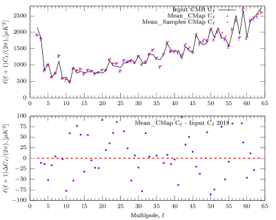
Figure 9: We show the angular power spectrum estimated from the ${\tt mean\_CMap}$ with violet points while the input CMB power spectrum is shown in black line. We see both the power spectra agree with each other. The power spectrum obtained after taking the mean of 10000 power spectra corresponding to the sampled mean maps is shown in red points.

We show our ${\tt mean\_CMap}$ in the top left panel of Figure 8. The difference between our ${\tt mean\_CMap}$ and the input CMB used is displayed in the top right panel of Figure 8. The residual map shows that our ${\tt mean\_CMap}$ matches very well with the CMB realization used in the simulation and our model is capable of recovering CMB signal quite well. The difference between the ${\tt bf\_CMap}$ and the ${\tt mean\_CMap}$ is shown in the bottom left panel of Figure 8 and the per-pixel error estimate corresponding to the ${\tt mean\_CMap}$ in the bottom right panel. The error map represents the standard deviation of the predictive posterior distribution of the CMB map.

Using the ${\tt mean\_CMap}$ we estimate the angular power spectrum after properly accounting for the beam and pixel effects and is shown in Figure 9 using violet points. The input CMB power spectrum is shown in black line. We see that our ${\tt mean\_CMap}$ power spectrum matches well with the input CMB power spectrum. From both the map and power spectrum comparisons we see that our model is able to accurately reconstruct a cleaned CMB map after minimizing the foregrounds present in the input simulated maps.

References

- Abadi et al. (2015) Abadi, M., Agarwal, A., Barham, P., et al. 2015, TensorFlow: Large-Scale Machine Learning on Heterogeneous Systems. https://www.tensorflow.org/
- Abazajian et al. (2022) Abazajian, K., et al. 2022. https://arxiv.org/abs/2203.08024
- Abdar et al. (2021) Abdar, M., Pourpanah, F., Hussain, S., et al. 2021, Information fusion, 76, 243
- Adak et al. (2022) Adak, D., Sen, A., Basak, S., et al. 2022, Mon. Not. Roy. Astron. Soc., 514, 3002, doi: 10.1093/mnras/stac1474
- Adams et al. (2023) Adams, J., Lu, S., Gorski, K. M., Rocha, G., & Wagstaff, K. L. 2023. https://arxiv.org/abs/2302.12378
- Ade et al. (2014) Ade, P. A. R., et al. 2014, Astron. Astrophys., 571, A1, doi: 10.1051/0004-6361/201321529
- Aghanim et al. (2020) Aghanim, N., et al. 2020, Astron. Astrophys., 641, A6, doi: 10.1051/0004-6361/201833910
- Allys et al. (2023) Allys, E., et al. 2023, PTEP, 2023, 042F01, doi: 10.1093/ptep/ptac150
- Bennett et al. (2003a) Bennett, C. L., Halpern, M., Hinshaw, G., et al. 2003a, ApJS, 148, 1, doi: 10.1086/377253
- Bennett et al. (2003b) Bennett, C. L., Hill, R. S., Hinshaw, G., et al. 2003b, ApJS, 148, 97, doi: 10.1086/377252
- Casas et al. (2022) Casas, J. M., Bonavera, L., González-Nuevo, J., et al. 2022, Astron. Astrophys., 666, A89, doi: 10.1051/0004-6361/202243450
- David M. Blei & McAuliffe (2017) David M. Blei, A. K., & McAuliffe, J. D. 2017, Journal of the American Statistical Association, 112, 859, doi: 10.1080/01621459.2017.1285773
- Defferrard et al. (2020) Defferrard, M., Milani, M., Gusset, F., & Perraudin, N. 2020, DeepSphere: a graph-based spherical CNN. https://arxiv.org/abs/2012.15000
- Delabrouille et al. (2009) Delabrouille, J., Cardoso, J. F., Le Jeune, M., et al. 2009, A&A, 493, 835, doi: 10.1051/0004-6361:200810514
- Eriksen et al. (2004) Eriksen, H. K., Banday, A. J., Górski, K. M., & Lilje, P. B. 2004, ApJ, 612, 633, doi: 10.1086/422807
- Eriksen et al. (2008a) Eriksen, H. K., Dickinson, C., Jewell, J. B., et al. 2008a, ApJ, 672, L87, doi: 10.1086/526545
- Eriksen et al. (2008b) Eriksen, H. K., Jewell, J. B., Dickinson, C., et al. 2008b, ApJ, 676, 10, doi: 10.1086/525277
- Farsian et al. (2020) Farsian, F., Krachmalnicoff, N., & Baccigalupi, C. 2020, JCAP, 07, 017, doi: 10.1088/1475-7516/2020/07/017
- Gal et al. (2017) Gal, Y., Hron, J., & Kendall, A. 2017, in Advances in Neural Information Processing Systems, ed. I. Guyon, U. V. Luxburg, S. Bengio, H. Wallach, R. Fergus, S. Vishwanathan, & R. Garnett, Vol. 30 (Curran Associates, Inc.). https://proceedings.neurips.cc/paper_files/paper/2017/file/84ddfb34126fc3a48ee38d7044e87276-Paper.pdf
- Górski et al. (2005) Górski, K. M., Hivon, E., Banday, A. J., et al. 2005, Astrophys. J., 622, 759, doi: 10.1086/427976
- Graves (2011) Graves, A. 2011, Advances in neural information processing systems, 24
- Gualtieri et al. (2018) Gualtieri, R., et al. 2018, J. Low Temp. Phys., 193, 1112, doi: 10.1007/s10909-018-2078-x
- He et al. (2015) He, K., Zhang, X., Ren, S., & Sun, J. 2015, arXiv e-prints, arXiv:1512.03385, doi: 10.48550/arXiv.1512.03385
- Hincks et al. (2010) Hincks, A. D., Acquaviva, V., Ade, P. A. R., et al. 2010, The Astrophysical Journal Supplement Series, 191, 423, doi: 10.1088/0067-0049/191/2/423
- Hoffman et al. (2013) Hoffman, M. D., Blei, D. M., Wang, C., & Paisley, J. 2013, Journal of Machine Learning Research, 14, 1303. http://jmlr.org/papers/v14/hoffman13a.html
- Hui et al. (2018) Hui, H., et al. 2018, Proc. SPIE Int. Soc. Opt. Eng., 10708, 1070807, doi: 10.1117/12.2311725
- Hurier et al. (2013) Hurier, G., Macías-Pérez, J. F., & Hildebrandt, S. 2013, A&A, 558, A118, doi: 10.1051/0004-6361/201321891
- Jaffe et al. (2006) Jaffe, T. R., Banday, A. J., Eriksen, H. K., Gorski, K. M., & Hansen, F. K. 2006, Astrophys. J., 643, 616, doi: 10.1086/501343
- Kingma & Ba (2014) Kingma, D. P., & Ba, J. 2014, arXiv e-prints, arXiv:1412.6980, doi: 10.48550/arXiv.1412.6980
- Kingma & Welling (2013) Kingma, D. P., & Welling, M. 2013, arXiv e-prints, arXiv:1312.6114, doi: 10.48550/arXiv.1312.6114
- Knowles (2015) Knowles, D. A. 2015, arXiv e-prints, arXiv:1509.01631, doi: 10.48550/arXiv.1509.01631
- Kullback & Leibler (1951) Kullback, S., & Leibler, R. A. 1951, The annals of mathematical statistics, 22, 79
- Land & Magueijo (2006) Land, K., & Magueijo, J. 2006, Mon. Not. Roy. Astron. Soc., 367, 1714, doi: 10.1111/j.1365-2966.2006.10078.x
- Lazear et al. (2014) Lazear, J., Ade, P. A. R., Benford, D., et al. 2014, in Society of Photo-Optical Instrumentation Engineers (SPIE) Conference Series, Vol. 9153, Millimeter, Submillimeter, and Far-Infrared Detectors and Instrumentation for Astronomy VII, ed. W. S. Holland & J. Zmuidzinas, 91531L, doi: 10.1117/12.2056806
- Lewis & Challinor (2011) Lewis, A., & Challinor, A. 2011, CAMB: Code for Anisotropies in the Microwave Background, Astrophysics Source Code Library, record ascl:1102.026
- Li et al. (2019) Li, H., et al. 2019, Natl. Sci. Rev., 6, 145, doi: 10.1093/nsr/nwy019
- Masi et al. (2002) Masi, S., et al. 2002, Prog. Part. Nucl. Phys., 48, 243, doi: 10.1016/S0146-6410(02)00131-X
- Montefalcone et al. (2021) Montefalcone, G., Abitbol, M. H., Kodwani, D., & Grumitt, R. 2021, Journal of Cosmology and Astroparticle Physics, 2021, 055, doi: 10.1088/1475-7516/2021/03/055
- Pal & Saha (2023) Pal, S., & Saha, R. 2023, J. Astrophys. Astron., 44, 84, doi: 10.1007/s12036-023-09974-4
- Pal et al. (2024) Pal, S., Yadav, S. K., Saha, R., & Souradeep, T. 2024. https://arxiv.org/abs/2404.18100
- Petroff et al. (2020) Petroff, M. A., Addison, G. E., Bennett, C. L., & Weiland, J. L. 2020, Astrophys. J., 903, 104, doi: 10.3847/1538-4357/abb9a7
- Ronneberger et al. (2015) Ronneberger, O., Fischer, P., & Brox, T. 2015, arXiv e-prints, arXiv:1505.04597, doi: 10.48550/arXiv.1505.04597
- Samuel (1959) Samuel, A. L. 1959, IBM Journal of Research and Development, 3, 210, doi: 10.1147/rd.33.0210
- Specht (1990) Specht, D. F. 1990, Neural Networks, 3, 109, doi: https://doi.org/10.1016/0893-6080(90)90049-Q
- Sudevan et al. (2017) Sudevan, V., Aluri, P. K., Yadav, S. K., Saha, R., & Souradeep, T. 2017, ApJ, 842, 62, doi: 10.3847/1538-4357/aa7334
- Taylor et al. (2006) Taylor, J. F., Ashdown, M. A. J., & Hobson, M. P. 2006, in 41st Rencontres de Moriond: Workshop on Cosmology: Contents and Structures of the Universe (Hanoi: The Gioi), 290–292
- Tegmark et al. (2003) Tegmark, M., de Oliveira-Costa, A., & Hamilton, A. J. 2003, Phys. Rev. D, 68, 123523, doi: 10.1103/PhysRevD.68.123523
- Thorne et al. (2017) Thorne, B., Dunkley, J., Alonso, D., & Naess, S. 2017, Mon. Not. Roy. Astron. Soc., 469, 2821, doi: 10.1093/mnras/stx949
- Tipping (2004) Tipping, M. E. 2004, Bayesian Inference: An Introduction to Principles and Practice in Machine Learning, ed. O. Bousquet, U. von Luxburg, & G. Rätsch (Berlin, Heidelberg: Springer Berlin Heidelberg), 41–62, doi: 10.1007/978-3-540-28650-9_3
- Wang et al. (2022) Wang, G.-J., Shi, H.-L., Yan, Y.-P., et al. 2022, Astrophys. J. Supp., 260, 13, doi: 10.3847/1538-4365/ac5f4a
- Wen et al. (2018) Wen, Y., Vicol, P., Ba, J., Tran, D., & Grosse, R. 2018, arXiv e-prints, arXiv:1803.04386, doi: 10.48550/arXiv.1803.04386
- Yan et al. (2024) Yan, Y.-P., Li, S.-Y., Wang, G.-J., Zhang, Z., & Xia, J.-Q. 2024. https://arxiv.org/abs/2406.17685
- Yan et al. (2023a) Yan, Y.-P., Wang, G.-J., Li, S.-Y., & Xia, J.-Q. 2023a, Astrophys. J., 947, 29, doi: 10.3847/1538-4357/acbfb4
- Yan et al. (2023b) —. 2023b, Astrophys. J. Suppl., 267, 2, doi: 10.3847/1538-4365/acd2ce
- Yi et al. (2020) Yi, K., Guo, Y., Fan, Y., Hamann, J., & Wang, Y. G. 2020. https://arxiv.org/abs/2001.11651