Staff Scheduling for Demand-Responsive Services

Abstract

Staff scheduling is a well-known problem in operations research and finds its application at hospitals, airports, supermarkets, and many others. Its goal is to assign shifts to staff members such that a certain objective function, e.g. revenue, is maximized. Meanwhile, various constraints of the staff members and the organization need to be satisfied. Typically in staff scheduling problems, there are hard constraints on the minimum number of employees that should be available at specific points of time. Often multiple hard constraints guaranteeing the availability of specific number of employees with different roles need to be considered.

Staff scheduling for demand-responsive services, such as, e.g., ride-pooling and ride-hailing services, differs in a key way from this: There are often no hard constraints on the minimum number of employees needed at fixed points in time. Rather, the number of employees working at different points in time should vary according to the demand at those points in time. Having too few employees at a point in time results in lost revenue, while having too many employees at a point in time results in not having enough employees at other points in time, since the total personnel-hours are limited. The objective is to maximize the total reward generated over a planning horizon, given a monotonic relationship between the number of shifts active at a point in time and the instantaneous reward generated at that point in time. This key difference makes it difficult to use existing staff scheduling algorithms for planning shifts in demand-responsive services.

In this article, we present a novel approach for modelling and solving staff scheduling problems for demand-responsive services that optimizes for the relevant reward function.

1 Introduction

Working time of the employees is a finite and valuable resource in most organizations. Therefore, planning shifts for the staff members in an optimal way is very important in a wide variety of industries, including transportation, hospitality, manufacturing and retail. Especially in settings where the demand for the goods or services provided varies with time, it is very important for the shift plan to ensure that the total deployed workforce at a point of time matches the demand well [20]: planning too few employees at a period of high demand leads to lost productivity, planning too many employees during low demand results in an opportunity cost.

The staff scheduling process often needs to take various constraints into account. Some of these constraints may be a consequence of limited availability of a physical resource, such as workspace and equipments [23, 5]. Some constraints may be legal in nature, e.g. specific amount of breaks between successive shifts, mandatory days off etc. Some constraints may be due to the need to maintain high job satisfaction among the staff [21, 15]: Certain staff members may want to work only during the morning or night, for example. Finding any shift plan subject to these constraints me be a difficult task, let alone one maximizing some reward function.

Certain application areas might require specific additional constraints and different objectives. Staff scheduling for transportation services [12] often involves spatial constraints on the starting and ending location of the shifts and conformity with a time table of operation. Nurse scheduling in hospitals as well as emergency services need to accommodate different categories of personnel (able to perform different functions), as well as fair distribution of day and night shifts [1, 18]. Many industries need to accommodate part time employees [22] working only certain days of the week.

Integer programming was introduced as a method of solving staff scheduling problems as early as 1954 [11], and various integer programming formulations have been proposed since then [17, 16, 4, 3, 9]. The number of decision variables in integer programming models may be very large in realistic settings [14], leading to very high runtimes. Therefore, various metaheuristics based methods have been studied for solving staff scheduling problems, such as genetic programming [1, 19], tabu search [14, 10] and simulated annealing [8, 12].

We refer the reader to the review articles [13, 2] for comprehensive surveys of the staff scheduling problem and its applications.

2 Demand Modelling for Staff Scheduling

Staff scheduling in various settings start with a demand modelling step [13, 20], where for each time step, a required number of active shifts are calculated. We will henceforth refer to this quantity as the desired supply. This is computed by first estimating future demand of the services provided by the organization. Then domain knowledge on how much demand can be served by how much supply is utilized to convert the estimated demand into the desired supply [11]. In the later stages of the shift scheduling process [13,  p. 6], where shifts are planned while maximizing a certain objective, deviations from the desired supply are penalized. Demand modelling, i.e. converting estimated demand to desired supply can be performed using various approaches [20], including the three described below.

Productivity standards

assuming the desired supply at each time step vary linearly with the demand at that time step.

Service standards

equating the desired supply to the number that achieves a constant fraction of the demand being served at each time step.

Economic standards

assigning a cost to each unit of workforce deployed at each time step, and assigning a reward to each unit of demand served at each time step, and choosing the supply that maximizes the reward minus the cost at that time step.

We note that both the service standards approach and the economic standards approach assumes that given a supply, i.e. the number of active shifts, and a demand, it is possible to determine the amount of demand that can be served or the amount of reward that can be generated. Crucially, the demand modelling step is usually performed without utilizing any knowledge of the available workforce [20].

3 Our Contribution: Integrating Demand Modelling and Shift Optimization into a Single Step

In this article, we present a novel approach for modelling and solving staff scheduling problems for demand-responsive services. We eliminate demand modelling as a separate step and incorporate it into a mixed-integer program producing optimal shift plans. Our approach maximizes the total reward (e.g. revenue) accumulated over the planning horizon, given that the relationship between the total number of active shifts at a point of time and the instantaneous reward is known and is concave. By eschewing the demand modelling step, our approach is able to achieve a higher value of total reward compared to what is possible with approaches where demand modelling is done in a separate step.

Our methods and results apply to a broad class of demand-responsive services satisfying the following criteria. First, the number of employees available during a planning horizon (e.g. a week) is fixed and is known a priori, and so are the numbers and lengths of shifts that must be assigned to each employee within the planning horizon. Second, there exists a metric whose sum total over the planning horizon is to be maximized by the staff scheduling process (this could be expected revenue, for example). Third, the metric is concave with respect to the number of active shifts at each point in time. However, this concave function need not be the same for all points in time.

We present a way to model the staff scheduling problem as a mixed-integer convex optimization problem. We also demonstrate a concrete example of this general approach for planning driver shifts for an demand-responsive mobility-as-a-service (MaaS) company. For sake of simplicity, we leave out the rostering step, where the planned shifts are assigned to individual employees, in this article.

4 Problem setting

For a natural number $n$, we denote by $[n]$ the set $\left\{1,\dots,n\right\}$. We consider a planning horizon (e.g. 7 days) which is discretized into $T$ time steps. We assume that at each time step, shifts of $k\geq 1$ different shift types can be started and each shift type $i\in[k]$ has a duration of $\delta_{i}\in\mathbb{N}$ time steps. Shift types may indicate, for example, different employee groups. As part of the shift planning process, we need to determine how many shifts of each type to start at which time step. To this end, for every shift type $i\in[k]$ and time step $t\in[T]$, we introduce a decision variable

$$x_{i,t}:=\text{ the number of shifts of type }i\text{ {starting} at time }t.$$ (1)

The number of active shifts of type $i$ at time $t$ is then given by

$$y_{i,t}=\sum_{\tau=t-\delta_{i}+1}^{t}x_{i,\tau}$$ (2)

and the total number of active shifts, or supply, at time $t$ is given by

$$y_{t}=\sum_{i=1}^{k}y_{i,t}.$$ (3)

Let the vector

$$\textbf{x}:=(x_{i,t})_{i\in[k],t\in[T]}$$ (4)

describe the shift plan. We assume that x is subject to linear constraints of the form $A\textbf{x}\leq\textbf{b}$ for some matrix $A$ and vector b of corresponding dimensions. Some of these constraints are needed to specify that the total working hours of the employees is a predetermined constant. Some rows of $A$ may indicate certain operational constraints the staff schedule must fulfil (e.g., the total number of simultaneous users of a physical resource must not be larger than the total number of that resource available).

The objective is to find a feasible shift schedule that maximizes a reward function over the planning horizon. Specifically, for each time step $t\in[T]$, we have a concave function $f_{t}\colon\mathbb{R}_{\geq 0}\to\mathbb{R}$ mapping the total number of active shifts $y_{t}$ at time $t$ to the instantaneous reward $r_{t}$,

$$r_{t} =f_{t}(y_{t}).$$ (5)

The objective is to maximize the total reward over the planning period $\sum_{t=1}^{T}r_{t}$.

Using Equation 2, the resulting mixed-integer convex problem can then be formulated as

$$\max\quad \sum_{t=1}^{T}f_{t}\left(\sum_{i=1}^{k}y_{i,t}\right)$$

s.t. $$y_{i,t}=\sum_{\tau=t-\delta_{i}+1}^{t}x_{i,\tau} \text{for all }i\in[k],\;t\in[T],$$

$$A\textbf{x}\leq\textbf{b}$$

$$x_{i,t}\in\mathbb{Z} \text{for all }i\in[k],\;t\in[T].$$

5 Application to shift planning for on-demand mobility

In on-demand mobility services such as MOIA, the number of vehicles deployed at a given point in time should vary according to the demand from the customers to avail the service at that time. The total number of deployed vehicles naturally is equal to the total number of driver shifts active at that time. The demand may not be exactly known when the shifts need to be planned, but can be estimated based on historical data.

Usually, the objective function that should be maximized by the shift planning optimization process is the total number of served customers over the whole planning period. Depending on the business model of the company, the objective function may be slightly different, but it stands to reason that the objective function is the sum over the time steps of a monotonically increasing function of the number of active shifts at each time step: Because the more shifts are active at a time step, the more customers can be served at that point of time. In addition, we make the assumption that the function is concave. Intuitively, this means that the marginal benefit of adding one more shift at a time step decreases with the number of active shifts at that time step. This is a reasonable assumption, since the more shifts are active at a time step, the more likely it is that the demand in the vicinity of a vehicle is already satisfied by another vehicle, and thus, the contribution of that vehicle to the total number of served customers is smaller.

Finally, we assume that the total number of drivers employed by the company is a known and fixed number.

5.1 The Variables and Constraints

Following the general problem setting in Section 4, we assume we have $k\geq 1$ different shift types, each with a fixed duration of $\delta_{i}$ time steps, $i\in[k]$. A shift type may specify various properties of the employees, e.g. the contract type of the driver (full-time, part-time, contracted etc.), the days of the week as well as the time of the day (day/night) the driver is available.

Then the monotonically increasing concave function $f_{t}$ maps $y_{t}$, the total number of shifts active at the time step $t$, to the instantaneous reward $r_{t}$ (e.g. number of trips served at that time step). We assume that the function $f_{t}$ is known (e.g. by estimation from historical data).

As described above, the decision variables are $x_{i,t}$, the number of shifts of type $i$ started at time $t$. Various legal and operational constraints may need to be considered when optimizing the shifts, for example:

• The total number of active shifts at a time may be bounded above by the total number of vehicles available.

• The total number of shifts of a certain type within a day must be bounded above by the total number of drivers with that shift type employed by the provider.

5.2 The shift types

Let the planning horizon be a week, and suppose that shifts may be started at the beginning of every hour, i.e. the number of time steps is $T=7\times 24=168$. For simplicity, we assume that there are only one kind of employees, each working in $s$ shifts of length $\delta$ hours each (typical examples are $s=5$ and $\delta=8$). Consequently, we have only one shift type of duration $\delta$ hours. Therefore $y_{t}=y_{1,t}$ and $x_{t}=x_{1,t}$. Let the number of employees be $N$. Then the total number of shifts within the planning horizon of one week is $sN$.

5.3 The reward function

It is reasonable to assume that the on-demand mobility provider is interested in maximizing the total number of served rides within the planning period. Then the monotonically increasing concave reward function $f_{t}$ should map the number of active shifts at time $t$ to the number of served rides at that time. The number of served rides, given the number of active shifts $y_{t}$, should depend on the number of demanded rides: that is, $f_{t}$ should be parametrized by the demanded rides $d_{t}$ at time $t$: $f_{t}=f_{t,d_{t}}$. Additionally, it stands to reason that, for a fixed number of active shifts, the number of served rides will not decrease with the number of demanded rides, i.e.,

$$\frac{\partial f_{t,d_{t}}(y_{t})}{\partial d_{t}}\geq 0\quad\text{for all }y_{t}\geq 0.$$ (6)

Also, since the number of served rides cannot exceed the number of demanded rides,

$$\lim_{y_{t}\to\infty}f_{t,d_{t}}(y_{t})\leq d_{t}.$$ (7)

The method of this article does not depend on the specific choice of $f_{t}$, so long as it is monotonically increasing and concave. For the sake of concreteness, we will presently make the following choice:

$$f_{t,d_{t}}(y_{t})=d_{t}\left(1-e^{-ay_{t}/d_{t}}\right),$$ (8)

for some $a>0$; see Figure 1 for a visual representation.

Figure 1: The reward $r_{t}$ as a function of supply $y_{t}$ as defined in (8) for $d_{t}=1$ and different values of the parameter $a$.

5.3.1 Demanded rides

The only remaining unknown in the reward function is the demanded rides for each time $t$. Since our approach does not assume any property of the demanded rides, we will assume that $d_{t}$ is a periodic function of time $t$ with daily and weekly seasonality. More precisely, we will assume that $d_{t}$ is given by the function

$$d_{t}=\frac{d_{\max}}{2}\left[1-\cos\left(\frac{\pi t}{12}\right)\right]\sin\left(\frac{\pi t}{T}\right),$$ (9)

see Figure 2 for a visual representation.

Figure 2: The demanded rides $d_{t}$ as a function of time $t$.

5.4 The constraints

5.4.1 Shift plan must match the number of employed drivers

Recall that we have $N$ employees, each working $s$ shifts of $\delta$ hours each. This imposes the constraint that the total number of shifts within the planning horizon must be $sN$,

$$\sum_{t=1}^{T}x_{t}=sN.$$ (10)

However, this constraint alone is too weak: it does not take into account the fact that a single employee cannot work more than one shift at a time. In fact, most workplaces have a policy that each employee needs to have a minimum break of, say, $\beta$ time steps between two consecutive shifts. We can accommodate these constraints by extending each shift by $\beta$ time steps and requiring that at any point in time, there are at most $N$ extended shifts active. More formally, we introduce auxiliary variables $z_{t}$ for $t\in[T]$, given by

$$z_{t}:=\sum_{\tau=t-\delta-\beta+1}^{t}x_{\tau},$$ (11)

and require them to satisfy the following constraints

$$z_{t}\leq N\quad\text{for all }t\in[T].$$ (12)

We note that for all $t\in[T]$, $x_{t}\leq z_{t}$, and therefore, (12) implies that

$$x_{t}\leq N\quad\text{for all }t\in[T].$$ (13)

We describe each extended shift $s$ by an interval $s=[t_{1},t_{2})$, where $t_{1}$ is the starting time of the shift and $t_{2}$ is $\beta$ time steps after the end of the shift, i.e. $t_{2}=t_{1}+\delta+\beta$. We say that two extended shifts $s_{1}$ and $s_{2}$ overlap if $s_{1}\cap s_{2}\neq\emptyset$.

Observation 1.

Let $D_{1}$ and $D_{2}$ be two drivers and $S_{1}$ and $S_{2}$ be the set of extended shifts assigned to $D_{1}$ and $D_{2}$, respectively. Let $G$ be the graph with node set $S_{1}\cup S_{2}$, where two extended shifts are connected by an edge iff they overlap. Then $G$ is bipartite with node sets $S_{1}$ and $S_{2}$ if and only if there is no overlap between any two extended shifts assigned to the same driver.

We can now prove that the constraints (10) and (12) are sufficient to ensure that the shift plan can be assigned to the drivers in a feasible way.

Lemma 1.

If (10) and (12) hold, then there exists an assignment of shifts to drivers such that each driver works exactly $s$ shifts of $\delta$ hours each, and each driver has a break of at least $\beta$ time steps between any two consecutive shifts.

Proof.

We split this proof into two parts. First, we show that a shift plan satisfying (10) and (12) can be assigned to $N$ drivers such that there is a break of at least $\beta$ time steps between any two shifts of a driver. In the second part, we show that the same shift plan can be assigned to $N$ drivers such that, additionally, each driver works exactly $s$ shifts of $\delta$ hours each.

Let x as defined in (4) be a shift plan that fulfills (10) and (12).

Part 1: Proof that the shift plan can be assigned to the drivers with adequate breaks between shifts

We note that, from (11),

$$z_{t}=\sum_{\tau=t-\delta-\beta+1}^{t}x_{\tau}=\sum_{\tau=t-\delta-\beta+1}^{t-1}x_{\tau}+x_{t}.$$ (14)

The first term on the right-hand side of (14) is the number of drivers who may not be assigned any new shift at time $t$, because they either have an ongoing shift or their last shift ended less than $\beta$ time steps ago. The constraint $z_{t}\leq N$ therefore guarantees that at time $t$, there are at least $x_{t}$ drivers who may be assigned a new shift.

Part 2: Proof that the shift plan can be assigned to the drivers with each driver working exactly $s$ shifts

Now assume we have an assignment of shifts to drivers such that each driver has a break of at least $\beta$ time steps between two consecutive shifts, and assume that not every driver works exactly $s$ shifts. Then, by (10), there must be a driver $D_{1}$ who works more than $s$ shifts and a driver $D_{2}$ who works less than $s$ shifts. Let $S_{1}$ be the extended shifts of driver $D_{1}$ and $S_{2}$ be the extended shifts of driver $D_{2}$. Then we have $|S_{1}|\geq|S_{2}|+2$.

Let $G$ be the graph with node set $S_{1}\cup S_{2}$, where two nodes are connected by an edge iff they overlap. By Observation 1, $G$ is bipartite with node sets $S_{1}$ and $S_{2}$. Since all extended shifts have the same length, any extended shift can overlap with at most two other extended shifts. Therefore, every node in $G$ has degree at most 2. As a consequence, every connected component of $G$ is a path or a cycle. In particular, every connected component contains a path with all nodes of that connected component.

Since $G$ is bipartite, for any such path $P$, we have $|S_{1}\cap P|-|S_{2}\cap P|\in\left\{-1,0,1\right\}$. Since $|S_{1}|\geq|S_{2}|+2$, there must be a path $P$ such that $|S_{1}\cap P|-|S_{2}\cap P|=1$. Define $P_{1}:=S_{1}\cap P$ and $P_{2}:=S_{2}\cap P$. Since $P$ is a path containing nodes only from a single connected component of $G$, there are no edges between $P$ and $(S_{1}\cup S_{2})\setminus P$. In particular, no edge exists between

• $S_{1}\setminus P$ and $P_{2}$, as well as

• $S_{2}\setminus P$ and $P_{1}$.

As a consequence, we can reassign the extended shifts in $P_{1}$ to $S_{2}$ and the extended shifts in $P_{2}$ to $S_{1}$, thereby creating the new assignments $S_{1}^{\prime}$ and $S_{2}^{\prime}$ of shifts among $D_{1}$ and $D_{2}$, with

$$S_{1}^{\prime} =(S_{1}\setminus P_{1})\cup P_{2},$$

$$S_{2}^{\prime} =(S_{2}\setminus P_{2})\cup P_{1},$$

satisfying the property that the resulting graph remains bipartite. By Observation 1, each driver still has a break of at least $\beta$ time steps between any two shifts. In this way, we have reduced the difference in number of shifts between $D_{1}$ and $D_{2}$ by 2. We can repeat this process until every driver works exactly $s$ shifts. ∎

Figure 3: Proof of Part 2 of Lemma 1. The dashed rectangle shows a connected component of the bipartite graph $G$. $P_{1}$ can $P_{2}$ can be swapped, keeping the graph bipartite, because there is no edge between the connected component and the rest of the graph.

We note that the proof of Lemma 1 is constructive, and therefore, we can use it to assign the shifts to the drivers in a feasible way.

5.4.2 Available vehicles constraint

If the number of vehicles available to the mobility provider is fixed, say, $c$ then we need another constraint: The total number of active shifts at any time must be less than $c$,

$$y_{t}\leq c,\quad\text{for all }t\in[T].$$ (15)

5.5 The Full Program

The problem to maximize the total reward over the planning horizon subject to shift and vehicle constraints can then be formulated as the following mixed-integer convex program.

$$\max\quad \sum_{t=1}^{T}f_{t}\left(y_{t}\right)$$ (16a)

s.t. $$y_{t}=\sum_{\tau=t-\delta+1}^{t}x_{\tau}, \text{for all }t\in[T],$$ (16b)

$$y_{t}\leq c, \text{for all }t\in[T],$$ (16c)

$$\sum_{t=1}^{T}x_{t}=sN,$$ (16d)

$$z_{t}=\sum_{\tau=t-\delta-\beta+1}^{t}x_{t}, \text{for all }t\in[T],$$ (16e)

$$z_{t}\leq N, \text{for all }t\in[T],$$ (16f)

$$x_{t}\geq 0 \text{for all }t\in[T],$$ (16g)

$$x_{t}\in\mathbb{Z} \text{for all }t\in[T],$$ (16h)

where

$$f_{t}(y_{t})=d_{t}\left(1-e^{-ay_{t}/d_{t}}\right)$$ (17)

and

$$d_{t}=d_{\max}\left[1+\sin\left(\frac{\pi t}{12}\right)\right].$$ (18)

For a better overview, we summarize the parameters of the mathematical program in the following table.

Parameter	Meaning
$T$	number of time steps in the planning horizon
$N$	number of employees
$s$	number of shifts each employee works
$\delta$	length of each shift
$\beta$	minimum break between two consecutive shifts
$d_{\max}$	maximum amplitude of the sinusoidal demand pattern
$a$	steepness of the concave function $f_{t}$

5.6 Benchmarking against shift agnostic optimum

Maximizing the total reward is the objective of the shift planning process we have described. If more constraints are imposed, the total optimum reward may decrease, yet those constraints may be necessary for operations, legal or strategic reasons. For an demand-responsive service provider, it is important to know how much is the cost of such constraints. To that end, we will now present a novel metric for evaluating the quality of a shift plan.

The shift agnostic optimum

Henceforth, we will assume that the reward functions $f_{t}$ are continuous for all $t\in[T]$. We define the shift agnostic optimum as the maximum reward that can be achieved, ignoring all the constraints and even ignoring the fact that the shifts are of fixed lengths, but keeping the total personnel working time fixed. Specifically, the shift agnostic optimum is defined as the optimal value of the following convex optimization problem:

$$\begin{split}\max\quad&\sum_{t=1}^{T}f_{t}\left(y_{t}\right)\\ \text{s.t.}\quad&\sum_{t=1}^{T}y_{t}=sN\delta,\\ &y_{t}\geq 0\quad\text{for all }t\in[T].\end{split}$$ (19)

Note that since the objective function of (19) is continuous and the feasible set is compact, the problem indeed has an optimal solution and the shift agnostic optimum is well-defined.

In the following lemma, we provide optimality conditions for problem (19) that will help us to derive explicit formulas for the shift agnostic optimum for the concrete example that we will study in the remainder of this paper.

Lemma 2.

Let the reward functions $f_{t}$ be continuously differentiable and concave for all $t\in[T]$. Then a vector $(y^{*}_{1},y^{*}_{2},\cdots,y^{*}_{T})$ is an optimal solution to the optimization problem (19) if and only if there exist constants $\lambda\in\mathbb{R}$ and $\mu_{1},\dots,\mu_{T}\in\mathbb{R}_{\geq 0}$ such that the following conditions hold:

$$\frac{\partial f_{t}(y^{*}_{t})}{\partial y_{t}}+\mu_{t} =\lambda, \text{for all }t\in[T]$$ (20)

$$\sum_{t=1}^{T}y^{*}_{t} =sN\delta,$$

$$y_{t}^{*} \geq 0, \text{for all }t\in[T],$$

$$y_{t}^{*}\mu_{t} =0, \text{for all }t\in[T].$$

If in addition $f_{t}$ is strictly concave for all $t\in[T]$, then the optimal solution is unique.

Proof.

The KKT conditions [7] guarantee that any solution to the maximization problem (19) must satisfy (20).

Since $f_{t}$ is concave for all $t\in[T]$, and all constraints are linear, the problem is convex, and thus, the above conditions also become sufficient.

Finally, if $f_{t}$ is strictly concave in $y_{t}$ for all $t$, then the objective function of problem (19) is strictly concave, and thus, the optimal solution is unique. ∎

For the particular choice of $f_{t}$ given by (8),

$$f_{t,d_{t}}(y_{t})=d_{t}\left(1-e^{-ay_{t}/d_{t}}\right),$$

the shift agnostic optimum is given by

$$y^{*}_{t}=\frac{sN\delta}{\sum_{\tau=1}^{T}d_{t}}d_{t},$$ (21)

which can be verified via equation system (20).

In the subsequent sections, we will use the shift agnostic optimum as a benchmark to compare our approach against. To that end, we define the relative gap from optimum supply as follows.

Definition 1 (Relative gap from optimum supply).

Let x be a shift plan with with total personnel time $sN\delta$, and let $y_{t}$ be the corresponding supply at time $t$. Let $r^{*}$ be the corresponding shift agnostic optimum, i.e., the optimum value of problem (19). Then the relative gap from optimum supply $\Delta(\textbf{x})$ is defined as the relative difference between the total reward of the shift plan x and the shift agnostic optimum,

$$\Delta(\textbf{x}) :=\frac{r^{*}-\sum_{t=1}^{T}f_{t}(y_{t})}{r^{*}}.$$ (22)

If $r^{*}>0$ and the reward functions $f_{t}$ are non-negative for all $t\in[T]$ (as it is the case for our particular choice of $f_{t}$ (8)), then $\Delta(\textbf{x})\in[0,1]$.

5.7 Benchmarking against approaches using a separate demand modelling step

Here we outline a method to compare the quality of the shift plans generated by the process described above with shift plans generated using a traditional demand modelling step [20]. As described in Section 2, these approaches first convert the demand to required working staff at each point of time. At the second step, the shift plans are generated by solving a mixed-integer convex problem that minimizes the sum of quadratic deviations from the required working staff at each point of time.

We will consider two different approaches for demand modelling described in Section 2: (a) service standards, and (b) economic standards, and compare the resulting shift plans from each approach with the approach we introduced.

Service standards

In this approach, the number of required working staff at each point is time is equated to the number that achieves a constant fraction of the demand being served. Assuming that the reward function (8) denotes the amount of served demand, maintaining a constant fraction $c\leq 1$ of the demand being served requires $y^{\text{s}}_{t}$ working staff at time $t$, where

$$f_{t}(y^{\text{s}}_{t})=cd_{t}.$$ (23)

Solving (23) for $y^{\text{s}}_{t}$ yields

$$y^{\text{s}}_{t}=ad_{t}\log{\frac{1}{1-c}}.$$ (24)

Economic standards

Maintaining a constant service standard may not be economically the best choice: A low service standard at low demand periods may lead to less lost revenue than a similarly low service standard at a high demand period. The economic standard approach attempts to tackle this problem by assigning a cost per deployed staff, as well as a reward (e.g. revenue) per served demand at each point in time. Then the number of required working staff at a point in time is obtained by the number of staff that maximizes the reward minus the cost, i.e.

$$y^{\text{e}}_{t}=\operatorname*{argmax}_{y\geq 0}\left\{f_{t}(y)-cy\right\},\quad\forall t\in[T],$$ (25)

where $c>0$ is the cost per deployed staff. Then for the choice of the reward function (8), (25) implies

$$y^{\text{e}}_{t}=\begin{cases}\frac{d_{t}}{a}\log{\frac{a}{c}},&\text{if }a>c,\\ 0,&\text{else}.\end{cases}$$ (26)

In both cases, the shift plan can then be computed by minimizing the deviation between the supply $y_{t}$ and the desired supply $y_{t}^{\prime}$, which is $y_{t}^{s}$ for service standards and $y_{t}^{e}$ for economic standards. Specifically, the shift plan is computed by solving the following mixed-integer quadratic program:

$$\min\quad \sum_{t=1}^{T}\left(y_{t}-y_{t}^{\prime}\right)^{2}$$ (27a)

s.t. $$y_{t}=\sum_{\tau=t-\delta+1}^{t}x_{\tau}, \text{for all }t\in[T],$$ (27b)

$$y_{t}\leq c, \text{for all }t\in[T],$$ (27c)

$$\sum_{t=1}^{T}x_{t}=sN,$$ (27d)

$$z_{t}=\sum_{\tau=t-\delta-\beta+1}^{t}x_{t}, \text{for all }t\in[T],$$ (27e)

$$z_{t}\leq N, \text{for all }t\in[T],$$ (27f)

$$x_{t}\geq 0 \text{for all }t\in[T],$$ (27g)

$$x_{t}\in\mathbb{Z} \text{for all }t\in[T].$$ (27h)

We have chosen the quadratic objective function (27a) instead of the sum of absolute deviations $\sum_{t=1}^{T}\left|y_{t}-y_{t}^{\prime}\right|$ because the former penalizes large deviations more than the latter.

6 Results

Now we present the results of solving the mixed-integer convex program described in Section 5.5, using the open source SCIP optimization suite [6]. To this end, we reduce the problem to a mixed-integer linear program (MIP) by first replacing the reward function $f_{t}$ defined in (17) with a piecewise linear concave approximation

$$f_{t}^{\prime}(y_{t})=\min\left\{h_{t,1}(y_{t}),\dots,h_{t,k}(y_{t})\right\},$$ (28)

where $h_{t,1},\dots,h_{t,k}$ are linear functions. The resulting program can then be transformed into the following MIP:

$$\max\quad \sum_{t=1}^{T}r_{t}$$ (29a)

s.t. $$r_{t}\leq h_{t,i}(y_{t})\quad\text{for all }i\in[k],\;t\in[T],$$ (29b)

$$\eqref{program:first-constraint}-\eqref{program:last-constraint}.$$ (29c)

We note that, in order to obtain an accurate approximation of the reward function $f_{t}$ while not increasing the number of variables and constraints too much, we may allow the number of linear segments $k$ in the piecewise linear approximation (28) to depend on the time $t$.

6.1 Solving the MIP to produce a shift plan

In the following, we will use the term shift agnostic optimum for both the optimal value as well as the optimal solution of the optimization problem (19), whenever it is clear from the context which one is meant. Figure 4 shows a solution to the MIP formulation (29) for $N=10$, $s=5$, $\delta=8$, $\beta=8$, $d_{\max}=10$, and $a=2$. The solution is reasonably close to the shift agnostic optimum, following the periodic demand pattern. However, the various shift constraints prevent the solution from perfectly matching the shift agnostic optimum. In particular, the solution does not have the smooth shape of the shift agnostic optimum, but is piecewise constant. Moreover, the solution does not reach the peak of the shift agnostic optimum in the middle of the week. In the following sections, we will investigate the impact of the various shift constraints on the quality of the solution and how relaxing them helps to overcome these limitations.

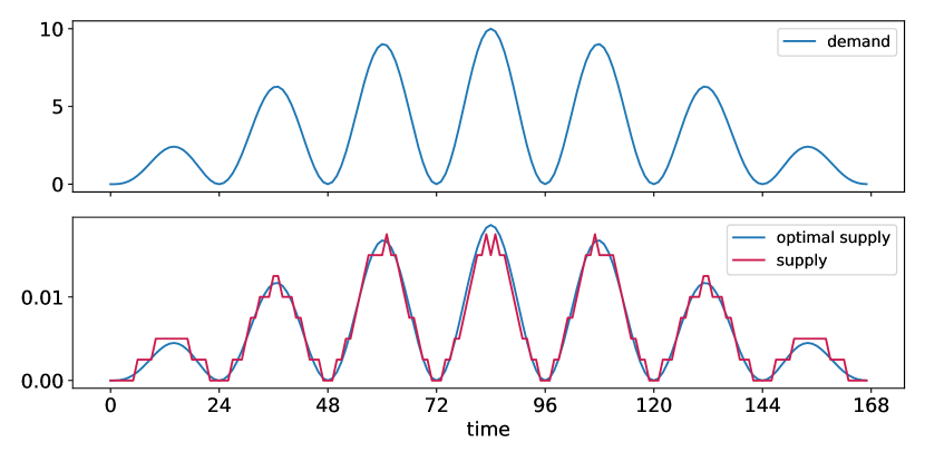
Figure 4: A solution to the MIP formulation (16) that is close to the shift agnostic optimum. Solved for $N=10$, $s=5$, $\delta=8$, $\beta=8$, $d_{\max}=10$, $a=2$.

6.2 Impact of different shift constraints on the gap between solution and shift agnostic optimum

In this subsection, we analyze the impact of various shift constraints on the quality of the optimum feasible shift plan. Specifically, we investigate the impact of the total number of drivers $N$, the number of shifts per driver $s$, and the shift length $\delta$ on the relative gap from optimum supply as defined in (22).

6.2.1 Impact of the total number of drivers

Since every started shift is active for $\delta$ time steps, the active shifts curve $\textbf{y}=(y_{t})_{t\in[T]}$ is the sum of $sN$ step functions. For a small number of drivers $N$, it is therefore difficult to approximate the smooth shift agnostic optimum $\textbf{y}^{*}=(y^{*}_{t})_{t\in[T]}$. As the number of drivers increases, the approximation becomes more accurate, and the gap between the solution y and the shift agnostic optimum $\textbf{y}^{*}$ decreases. Figure 5 illustrates this effect. For an increasing number of drivers $N$, we computed the corresponding optimal shift plan x and its supply curve y as well as the shift agnostic optimum $\textbf{y}^{*}$. For comparability, we normalized each supply curve by dividing it by the total working hours $sN\delta$.

For each number of drivers, we have computed the served trips using (8), and also the served trips for the shift agnostic optimum. The gap between the two is then the lost trips due to shift restrictions.These lost trips, divided by the total served trips due to the shift agnostic optimum, i.e. the relative gap from optimum supply as defined in (22), are plotted in panel (b) of Figure 5. We observe that the higher the number of drivers, the smoother the supply curve of the optimal shift plan and the smaller the relative gap from optimum supply. Notice, however, that even for as many as 200 drivers, the shift agnostic optimum is not reached. The reason for this is that, since every driver needs to work $s$ shifts per week, only $1/s$ of the total number of shifts can be active at the same time. Thus, the high peak in the middle of the week cannot be completely fulfilled. This limitation can be overcome by reducing the number of shifts per driver, as we will see in the next section.

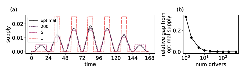
Figure 5: As the number of drivers $N$ increases, the difference between the shift agnostic optimum and the optimal shift plan decreases. (a) The supply curve, for different values of total drivers (coloured dashed lines), as well as the shift agnostic optimum (solid black line). Each supply curve is normalized, i.e., divided by the total working hours $sN\delta$. (b) The relative gap from optimum supply compared to the shift agnostic optimum, which decreases as the number of drivers increases.

6.2.2 Impact of weekly shifts per driver

If the total working time $sN\delta$ and the shift length $\delta$ is fixed but both the number of drivers $N$ and the number of shifts per driver $s$ are flexible, then it is beneficial to choose more drivers with fewer shifts; see Figure 6. As an intuitive example, consider two scenarios, one with $N$ drivers with $s$ shifts each, and another with $sN$ drivers with only one shift each. Then any shift plan for the first scenario can also be realized in the second scenario by assigning each of the $s$ shifts of a driver in the first scenario to $s$ different drivers in the second scenario. Therefore, the optimal shift plan in the second scenario is at least as good as the optimal shift plan in the first scenario. Moreover, while in the first scenario only $N$ shifts can be active at the same time, in the second scenario $sN$ shifts can be active at the same time, allowing to reach higher peaks.

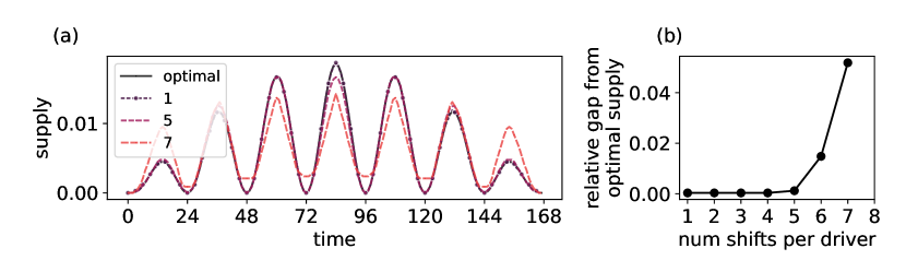
Figure 6: As the number of shifts per driver $s$ decreases, the difference between the shift agnostic optimum and the optimal shift plan decreases.

6.2.3 Impact of shift lengths

Finally, if the total working time $sN\delta$ and the number of shifts per driver $s$ is fixed but both the shift length $\delta$ and the number of drivers $N$ are flexible, then it is beneficial to choose more drivers with shorter shifts. In this way, we have more step functions with smaller support that can approximate the smooth shift agnostic optimum better; see Figure 7. Consider, for example, five different choices of shift length, $\delta\in\left\{1,2,4,8,16\right\}$. Then any solution with a shift length of $\delta=2^{i}$, $i>0$, and $N$ drivers can also be realized by $2N$ drivers with shift length $\delta^{\prime}=\delta/2$ by substituting each shift of length $\delta$ with two shifts of length $\delta^{\prime}$. Therefore, the smaller $i$ is, the better the resulting solution.

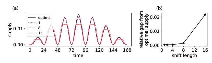
Figure 7: As the shift length $\delta$ decreases, the difference between the shift agnostic optimum and the optimal shift plan decreases.

6.3 Comparison to approaches with a separate demand modelling step

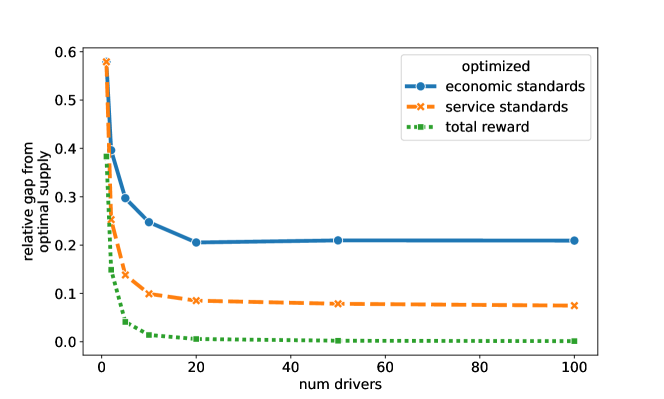
Figure 8: Our shift planning method achieves higher total reward than approaches with a separate demand modelling step. We have plotted the relative gap from optimum supply (21) for different values of the number of drivers $N$. All three approaches achieve smaller relative gap from optimum supply as the number of drivers increases, but our approach achieves the least relative gap from optimum supply for all values of $N$. For service standards, the parameter $c$ was set to $0.8$, and for economic standards, the parameter $c$ was set to $1$. Other parameters were set to $s=5$, $\delta=8$, $\beta=9$, $d_{\max}=0.75N$, $a=2$.

To demonstrate the benefit of combining the demand modelling with the shift plan optimization in one step, we now compare the quality of the shift plans generated by our method with ones generated by the two approaches with separate demand modelling steps described in Section 5.7. As before, we will use the relative gap from optimum supply as the metric for these comparisons.

We see in Figure 8 that the quality of the shift plans generated by both of these approaches lead to significantly less total reward than the ones generated by our approach. This stems from the fact that our approach as described in the problem formulation (16) directly maximizes the total served trips, thereby minimizing the relative gap from optimum supply. Both of the other approaches, by the very nature of having a separate demand modelling step, first compute the desired supply, and then minimize the deviation from that. This two-step process leads to a loss of information, since the deviation from the desired supply does not capture the resulting lost revenue: The same deviation at different points in time can result in different amounts of lost revenue depending on the demand pattern. As a result the two-step optimization process does in general not maximize the total served trips.

Robustness of traditional approaches with internal parameters

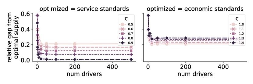
Figure 9: Staff scheduling approaches with demand modelling for both service standards and economic standards are highly dependent on the choice of the internal parameters. We have plotted the relative gap from optimum supply for both approaches, for different choices of the internal parameter $c$.

We also see in Figure 9 that the quality of the shift plans is highly dependent on the choice of service parameter in (24) for the service standards approach, and on the choice of the cost parameter in (25) for the economic standards approach. This demonstrates another advantage of our approach of directly maximizing the total reward, namely that it is not dependent on any such internal parameters.

7 Outlook

In this article we have introduced a novel approach to staff scheduling, where the total reward over the planning period is directly maximized, instead of first computing a desired supply by a demand modelling step. For showcasing the benefits of our approach, we chose a scenario with only one shift type and an exponential reward function, for the sake of simplicity. It will be interesting to study how our approach performs in more complex scenarios.

More complex reward function and shift types

First of all, it would be interesting to apply our approach to scenarios with more than one shift type. This would require generalizing the constraints (12) and Lemma 1 to ensure that the optimized shift plan is rosterable. Also, we have so far not considered breaks within a shift, but this can be easily accommodated by redefining active shifts in (2).

If the reward function is not concave in certain bounded subsets of its domain, often it is possible to approximate it with a concave approximation, e.g. by using the concave hull of a piecewise linear approximation. How the improvement of using our approach depends on the choice of the reward function is also an interesting question.

Further, it might be the case that the different shift types contribute in different ways to the reward function. For example, full-time employees might be more experienced and thus more productive than employees only working a few hours per week. In this case, instead of letting the reward function $f_{t}$ only depend on the aggregated supply $y_{t}=\sum_{i\in[k]}y_{t,i}$, one can use a reward function $f_{t}(y_{t,1},\dots,y_{t,k})$ that directly depends on the supply of each shift type. If it is possible to express the reward function as $f_{t}(y_{t,1},\dots,y_{t,k})=\sum_{i\in[k]}f_{t,i}(y_{t,i})$, and all of the functions $f_{t,i}$ are concave, then the results of this article can easily be extended to this more general case.

Instead of only maximizing the total reward, a company might also want to maximize other metrics at the same time, for example, to achieve the right trade-off between total revenue and service quality. It would be interesting to extend our method to such use cases by applying techniques from multicriteria optimization.

Extending our approach to shift assignment

In this article, we have limited ourselves to producing a shift plan without assigning the shifts to individual employees. For only one shift type, as we have considered in Section 5, the proof of Lemma 1 can readily be turned into an algorithm for shift assignment. A generalization of Lemma 1 and an algorithm for shift assignment to multiple shift types is left for future research. We note that a different approach for assigning shifts to employees is to redefine shift types as described in Section 4 so that each shift type corresponds to shifts from a single employee. However, this comes at the cost of a larger optimization problem.

8 Conclusion

We have presented a novel approach to staff scheduling in this article, where the total reward over the planning period is directly maximized, instead of first computing a desired supply by a demand modelling step and then minimizing the deviation from that. We have shown that our approach leads to higher total reward than the traditional approaches. We have also presented a novel metric for evaluating the impact of constraints on the quality of a shift plan, the relative gap from optimum supply.

9 Declaration of interests

We acknowledge that Debsankha Manik and Rico Raber are employed at the ride-pooling operator MOIA.

References

- [1] Uwe Aickelin and Kathryn A Dowsland “Exploiting problem structure in a genetic algorithm approach to a nurse rostering problem” In Journal of scheduling 3.3 Wiley Online Library, 2000, pp. 139–153
- [2] Hesham K Alfares “Survey, categorization, and comparison of recent tour scheduling literature” In Annals of Operations Research 127 Springer, 2004, pp. 145–175
- [3] Nicholas Beaumont “Scheduling staff using mixed integer programming” In European journal of operational research 98.3 Elsevier, 1997, pp. 473–484
- [4] Stephen E Bechtold and Larry W Jacobs “Implicit modeling of flexible break assignments in optimal shift scheduling” In Management Science 36.11 INFORMS, 1990, pp. 1339–1351
- [5] Oded Berman, Richard C Larson and Edieal Pinker “Scheduling workforce and workflow in a high volume factory” In Management Science 43.2 INFORMS, 1997, pp. 158–172
- [6] Ksenia Bestuzheva et al. “The SCIP Optimization Suite 8.0”, 2021 URL: http://www.optimization-online.org/DB_HTML/2021/12/8728.html
- [7] Stephen P Boyd and Lieven Vandenberghe “Convex optimization” Cambridge university press, 2004
- [8] Michael J Brusco and Larry W Jacobs “A simulated annealing approach to the solution of flexible labour scheduling problems” In Journal of the Operational Research Society 44 Springer, 1993, pp. 1191–1200
- [9] Michael J Brusco and Larry W Jacobs “Starting-time decisions in labor tour scheduling: An experimental analysis and case study” In European Journal of Operational Research 131.3 Elsevier, 2001, pp. 459–475
- [10] Luís Cavique, César Rego and Isabel Themido “Subgraph ejection chains and tabu search for the crew scheduling problem” In Journal of the Operational Research Society 50 Springer, 1999, pp. 608–616
- [11] George B Dantzig “A comment on Edie’s “Traffic delays at toll booths”” In Journal of the Operations Research Society of America 2.3 INFORMS, 1954, pp. 339–341
- [12] A Ernst, Mohan Krishnamoorthy and Denis Dowling “Train crew rostering using simulated annealing” In Proceedings of ICOTA 98, 1998
- [13] Andreas T Ernst, Houyuan Jiang, Mohan Krishnamoorthy and David Sier “Staff scheduling and rostering: A review of applications, methods and models” In European journal of operational research 153.1 Elsevier, 2004, pp. 3–27
- [14] Fred Glover and Claude McMillan “The general employee scheduling problem. An integration of MS and AI” In Computers & operations research 13.5 Elsevier, 1986, pp. 563–573
- [15] Lynn Gordon and Erhan Erkut “Improving volunteer scheduling for the Edmonton Folk Festival” In Interfaces 34.5 INFORMS, 2004, pp. 367–376
- [16] Larry W Jacobs and Michael J Brusco “Overlapping start-time bands in implicit tour scheduling” In Management Science 42.9 INFORMS, 1996, pp. 1247–1259
- [17] Elbridge Gerry Keith “Operator scheduling” In AIIE Transactions 11.1 Taylor & Francis, 1979, pp. 37–41
- [18] M Mohammadian, M Babaei, M Amin Jarrahi and E Anjomrouz “Scheduling nurse shifts using goal programming based on nurse preferences: a case study in an emergency department” In International Journal of Engineering 32.7 MaterialsEnergy Research Center, 2019, pp. 954–963
- [19] Julio Tanomaru “Staff scheduling by a genetic algorithm with heuristic operators” In 1995 IEEE International Conference on Systems, Man and Cybernetics. Intelligent Systems for the 21st Century 3, 1995, pp. 1951–1956 IEEE
- [20] Gary M Thompson “Labor scheduling, part 2: Knowing how many on-duty employees to schedule” In Cornell Hotel and Restaurant Administration Quarterly 39.6 Sage Publications Sage CA: Thousand Oaks, CA, 1998, pp. 26–37
- [21] Gary M Thopsn “Labor scheduling, part 3: Developing a workforce schedule” In Cornell Hotel and Restaurant Administration Quarterly 40.1 Sage Publications Sage CA: Thousand Oaks, CA, 1999, pp. 86–96
- [22] AJ Vakharia, HS Selim and RR Husted “Efficient scheduling of part-time employees” In Omega 20.2 Elsevier, 1992, pp. 201–213
- [23] Xinhui Zhang and Jonathan F Bard “Equipment scheduling at mail processing and distribution centers” In IIE Transactions 37.2 Taylor & Francis, 2005, pp. 175–187