Scalable approach to monitored quantum dynamics and entanglement phase transitions

Abstract

Measurement-induced entanglement phase transitions in monitored quantum circuits have stimulated activity in a diverse research community. However, the study of measurement-induced dynamics, due to the requirement of exponentially complex postselection, has been experimentally limited to small or specially designed systems that can be efficiently simulated classically. We present a solution to this outstanding problem by introducing a scalable protocol in $U(1)$ symmetric circuits that facilitates the observation of entanglement phase transitions directly from experimental data, without detailed assumptions of the underlying model or benchmarking with simulated data. Thus, the method is applicable to circuits which do not admit efficient classical simulation and allows a reconstruction of the full entanglement entropy curve with minimal theoretical input. Our approach relies on adaptive circuits and a steering protocol to approximate pure-state trajectories with mixed ensembles, from which one can efficiently filter out the subsystem $U(1)$ charge fluctuations of the target trajectory to obtain its entanglement entropy. The steering protocol replaces the exponential costs of postselection and state tomography with a scalable overhead which, for fixed accuracy $\epsilon$ and circuit size $L$, scales as $\mathcal{N}_{s}\sim L^{5/2}/\epsilon$.

I introduction

Quantum dynamics and phase transitions in monitored quantum circuits have rapidly stimulated an avalanche of interest, bringing together researchers of quantum information, statistical physics and condensed matter physics [1, 2, 3, 4, 5, 6, 7]. The topic bridges multiple fields, providing a treasure trove of new phenomena and concepts. Moreover, these developments have concretely demonstrated that some of the most fascinating realizations of quantum matter are presently provided by the emerging Noisy Intermediate-scale Quantum (NISQ) devices [8].

The interest towards monitored circuits exploded after the discovery of measurement-induced entanglement phase transitions [9, 10, 11, 12]. The proliferation of entanglement due to local entangling operations is first hindered, and then completely halted, by measurement of a fraction of the qubits in the system. This manifests in a phase transition between the entanglement entropy volume-law and area-law phases when the measured fraction is increased. However, direct experimental approaches to entanglement phase transitions face two fundamental obstacles. First, a direct measurement of entanglement entropy requires quantum state tomography, the cost of which scales exponentially with system size, an issue already faced in some recent experiments [13, 14, 15]. The second, and more serious, bottleneck is posed by the exponential postselection problem [3]: to extract the properties of a quantum state resulting from monitored dynamics, one needs to prepare an ensemble of states with precisely the same measurement outcomes throughout the temporal evolution. Even for modest systems of 10-20 qubits, the cost of preparing a postselected ensemble soon becomes astronomical.

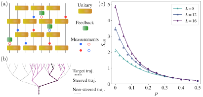
Figure 1: Scalable quantum simulation of entanglement in monitored quantum circuits with $U(1)$ symmetry. a, The studied brickwork circuits with two-qubit random unitaries and projective measurements. To implement steering towards a chosen target state, conditional single-qubit feedforward gates are applied to locally correct the state after measurements to match those of the target trajectory. b, Schematic illustration of branching of quantum trajectories by measurements, and steering them towards the target trajectory. c, Comparison of the exact trajectory-averaged entanglement entropy (solid lines) and the output of the protocol developed in this work (markers).

The existing workarounds to experimentally probe the transition rely on relaxing the postselection condition and pinpointing the transition by cross-referencing the measurement data with classical simulation data and theoretical mappings [16, 17, 18, 19, 20, 21, 22, 23, 24]. They can be regarded as hybrid experimental-theoretical approaches which rely heavily on theoretical assumptions on the underlying experimental systems and typically require that the systems can be efficiently simulated classically, involve heavy post-processing and provide only partial information of the entanglement dynamics.

In this work we introduce a scalable quantum simulation approach to reconstructing the entanglement entropy in $U(1)$-symmetric monitored circuits without exponential cost from either postselection or quantum state tomography. Our approach, illustrated in Fig. 1, employs adaptive circuits to remove the need for exponential postselection. We show how the relevant properties of a single quantum trajectory can be efficiently filtered from experimental data. Thus, our work establishes a scalable method to observing the measurement-induced entanglement phase transitions directly from the experimental data, without requiring classical benchmarking or detailed assumptions of the experimental system. With minimal theoretical input, our procedure also allows a full reconstruction of the entanglement entropy curve for all measurement rates.

II Entanglement dynamics from $U(1)$ charge fluctuations

II.1 Full postselection

To set the stage, we briefly review how the entanglement entropy can be extracted from the $U(1)$ charge fluctuations in $U(1)$ symmetric circuits as discussed in Refs. [25, 26]. The studied model consist of a linear array of $L$ qubits. At each time step, the system is evolved by applying unitary two-qubit gates followed by projective single-qubit measurements. The two-qubit gates, at even and odd time steps, act on qubits connected by even and odd links, as seen in Fig. 1. The successive odd and even time steps constitute a full cycle $t$. Without measurement, the evolution of a cycle is generated by

$${\bf U}(t)=\prod_{\text{even }n}U_{n,n+1}(2t)\prod_{\text{odd }n}U_{n,n+1}(2t-1)$$ (1)

where $U_{n,n+1}(\tau)$ is a two-qubit unitary acting on qubits at positions $n$ and $n+1$ at time step $\tau=2t\>\rm{or}\>2t-1$. To implement the $U(1)$ charge $Z_{L}=\sum_{n}Z_{n}$ conservation, where $Z_{n}$ is the Pauli-Z matrix operating on the $n$’th qubit, these unitary gates take the form

$$U_{n,n+1}=\begin{pmatrix}e^{i\varphi_{00}}&&\\ &e^{i\varphi_{11}}&\\ &&{\cal U}_{2\times 2}\end{pmatrix}$$ (2)

in the basis $\{\left|00\right\rangle,\left|11\right\rangle,\left|01\right\rangle$, $\left|10\right\rangle\}$. Here ${\cal U}_{2\times 2}$ is a generic $2\times 2$ unitary matrix constituting of four independent phases. Each local unitary gate $U_{n,n+1}(\tau)$ is chosen randomly and independently, by sampling all six phases that parameterize it from a uniform random distribution. Then, single-qubit measurements occur at the end of each half-cycle over randomly-chosen qubits with probability $p$. These measurements make the full dynamics non-unitary and inherently probabilistic. Considering single-qubit projective measurements, the wave function randomly collapses to an eigenstate of the corresponding single-qubit observable $\left|\Psi\right\rangle\to\frac{1}{\lVert P_{n,\alpha}\left|\Psi\right\rangle\rVert}P_{n,\alpha}\left|\Psi\right\rangle$ with projectors $P_{n,\alpha}$ acting on the qubit $n$ and satisfying normalization $\sum_{\alpha}P_{n,\alpha}={\mathbb{I}}$. We assume all measurements are performed in the $Z$-basis with the projectors $P_{n,\pm}=\big{(}{\mathbb{I}}\pm Z_{n}\big{)}/2$. Each set of particular measurement outcomes ${\bf m}\in\{1,-1\}^{M}$, where $M$ qubits are measured during the evolution, defines a unique quantum trajectory throughout which the state remains pure. The evolved state for any single realization of the monitored circuit can be denoted by $\left|\Psi\right\rangle_{\bf U,m}$ for a given random set of unitaries ${\bf U}$ and measurement outcomes ${\bf m}$.

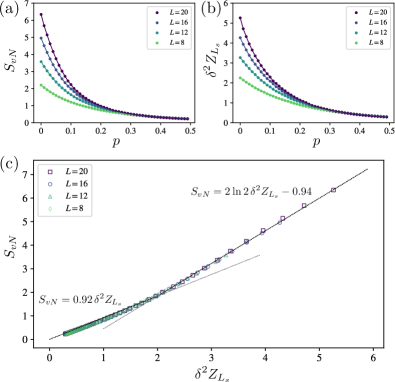
Figure 2: Pure state fluctuation-entanglement correspondence. a, Trajectory-averaged entanglement entropy as a function of the single-qubit measurement rate. b, Same as a but for the subsystem charge fluctuations. c, Universal variance-entropy relation, which is excellently approximated by two linear regimes.

To study the entanglement dynamics, we choose the initial state $\left|\Psi\right\rangle=\left|\uparrow\downarrow\uparrow\downarrow\cdots\uparrow\downarrow\right\rangle$, which, due to conservation, fixes the total $U(1)$ charge to zero $Z_{L}=\sum_{n}Z_{n}=0$. The von Neumann entanglement entropy for a subsystem with length $L_{s}$ is $S_{\text{vN}}=-{\rm Tr}\big{(}\rho_{s}\ln\rho_{s}\big{)}$, where the reduced density matrix $\rho_{s}$ is obtained from a pure state quantum trajectory by tracing out the complement as $\rho_{s}={\rm Tr}_{\bar{s}}(\left|\Psi\right\rangle\left\langle\Psi\right|)$. Below we exclusively consider partitions which divide the system in half $L_{s}=L/2$. As shown in Ref. [25], the entanglement entropy exhibits a phase transition between a volume-law and an area-law phase at $p=p_{c}\approx 0.14$ with the critical exponent $\nu\approx 1.3$. Moreover, the fluctuations $\delta^{2}Z_{L_{s}}=\langle Z_{L_{s}}^{2}\rangle-\langle Z_{L_{s}}\rangle^{2}$ of the subsystem $U(1)$ charge $Z_{L_{s}}=\sum_{n\in L_{s}}Z_{n}$ exhibit the same behaviour as the entanglement entropy, as is illustrated in Fig. 2a-b. As seen in Fig. 2c and discussed in Sec. I in Supplementary Information (SI), the entanglement entropy is a system size- and $p$-independent universal function of the variance $S_{\text{vN}}=f\left(\delta^{2}Z_{L_{s}}\right)$ which, to excellent approximation, is piecewise linear $S_{\text{vN}}=a\,\delta^{2}Z_{L_{s}}$ for $0\leq\delta^{2}Z_{L_{s}}\leq 2$ and $S_{\text{vN}}=2\ln 2\,\delta^{2}Z_{L_{s}}+(2a-4\ln 2)$ for $\delta^{2}Z_{L_{s}}>2$ with $a=0.92$. While the entanglement phase transition can be directly obtained from fluctuations, the variance-entropy relation allow a simple reconstruction of the full entanglement curve when $\delta^{2}Z_{L_{s}}$ is known.

II.2 Relaxing the exponential postselection by steering

As seen above, the fluctuations of the $U(1)$ charge allows one to access the entanglement entropy of pure states without exponential complexity associated with the state tomography. Nevertheless, one still has to deal with the postselection problem over quantum trajectories $\left|\Psi\right\rangle_{\bf U,m}$ corresponding to specific unitaries and $2^{M}$ different possible measurement outcomes ${\bf m}$. To enable fully scalable experimental studies of measurement-induced dynamics, we need a procedure to simulate properties of a single target quantum trajectory $\left|\Psi_{\bf U,m}\right\rangle$ without the need for exponential postselection. Instead of running the circuit exponentially many times in the hope of reproducing the target trajectory multiple times, we adopt the adaptive steering protocol depicted in Fig. 1b and summarized in Fig. 3. During the circuit execution, whenever the obtained measurement outcome differs from the one in the target trajectory, the circuit performs a Pauli-X operation on the measured qubit. This operation locally steers the outcomes immediately after measurements to match those of the target trajectory, ${\bf m}$. Repeating the steering evolution $\mathcal{N}_{s}$ times, each time we get a possibly different state $\left|\Psi_{{\bf m}^{\prime}_{i}\to{\bf m}}\right\rangle$ where ${\bf m}^{\prime}_{i}$ denotes the measurement outcomes in the $i$’th run. Without any postselection, the repetition of steering runs results in a mixed ensemble $\rho_{\bf U,m}=\frac{1}{\mathcal{N}_{s}}\sum_{i}\left|\Psi_{{\bf m}^{\prime}_{i}\to{\bf m}}\right\rangle\left\langle\Psi_{{\bf m}^{\prime}_{i}\to{\bf m}}\right|$ associated with the target state $\left|\Psi_{\bf U,m}\right\rangle$ . Steering processes by Pauli-X operators break the $U(1)$ charge conservation, creating an incoherent mixture of charge sectors during the evolution. However, the density matrix still commutes with the total charge, $[\rho_{\bf U,m},Z_{L}]=0$, and can be block-diagonalized in the total charge sectors. This allows for the separation of the steered states according to their total charge $Z_{L}$, resulting in steered ensembles, $\tilde{\rho}_{\bf U,m}^{Z_{L}}=\frac{1}{\mathcal{N}_{Z_{L}}}\sum^{\prime}_{i}\left|\Psi_{{\bf m}^{\prime}_{i}\to{\bf m}}\right\rangle\left\langle\Psi_{{\bf m}^{\prime}_{i}\to{\bf m}}\right|$ by summing over the states having a fixed total charge. We see that this way we can generate a mixed state which approximates the statistical properties of target states.

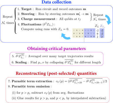
Figure 3: Summary of the scalable steering protocol. It provides the recipe to observe entanglement phase transitions and reconstruct the entanglement entropy in monitored circuits.

While the reduced von Neumann entropy is no longer an appropriate measure of entanglement for a mixed state, we now illustrate how to extract the postselected charge fluctuations from the fluctuations of the steered ensemble $\tilde{\rho}_{\bf U,m}^{Z_{L}}$. Since the postselected fluctuations immediately yield the entanglement entropy, as shown in Fig. 2c, this is the reason why our steering protocol provides access to the entanglement entropy. The main issue which needs to be resolved is that the fluctuations of the steered ensemble contain an additional incoherent contribution which is expected to lead to parasitic volume-law fluctuations. As discussed in Sec. II in the SI, this parasitic contribution is smaller for the charge-sector filtered ensembles $\tilde{\rho}^{Z_{L}}$ compared to the full steering mixture $\rho$ (we have dropped the subscripts for simplicity). Specifically, as shown in Fig. 4a, the fluctuations corresponding to $\tilde{\rho}^{Z_{L}=0}$ provide an excellent approximation of the postselected fluctuations in the volume-law regime. In the area-law regime, however, the incoherent contribution has to be explicitly subtracted. As discussed in Sec. III in SI, the incoherent fluctuations can be easily distinguished from the area-law contribution due to their different system-size dependency.

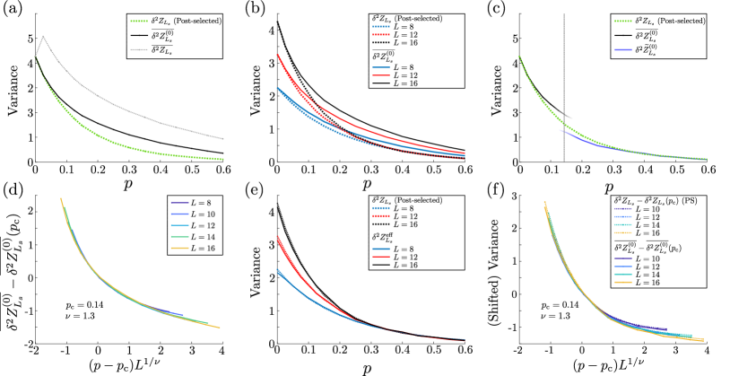
Figure 4: Extracting postselected quantities and entanglement phase transitions from steered ensembles. a, Subsystem charge fluctuations as a function of the measurement rate for $15\times 1000$ target trajectories (see Methods for details). Comparison of postselected data (dotted line) with the value obtained from the full steered ensemble $\delta^{2}Z_{L_{s}}^{\forall Z_{L}}$ and the $Z_{L}=0$ sector value $\delta^{2}Z_{L_{s}}^{(0)}$ for system size $L=16$. b, Comparison of the postselected and the $Z_{L}=0$ sector fluctuations for system lengths $8,12,16$, illustrating the parasitic volume contribution in the regime which for postselected data obeys the area law. c, Postselected data at $L=16$ compared to both $\delta^{2}Z_{L_{s}}^{Z_{L}=0}$, which is a good approximation for low $p$, and to the area-law corrected term $\delta^{2}Z_{L_{s}}^{Z_{L}=0}-c_{V}(p)$ which is a good approximation at high $p$. Around $p_{c}$, shown as a vertical line, they each deviate from the postselected value. d, Scaling collapse of the $Z_{L}=0$ sector fluctuations, which exhibit criticality with the same $p_{\mathrm{c}}$ and $\nu$ as the postselected fluctuations. e, Comparison of postselected fluctuations (dotted lines) and the effective fluctuations (solid lines) obtained through Eq. (4) for system lengths $L=8,12,16$. For the clarity, odd subsystem lengths have been excluded; the match is equally good for those. f, Scaling collapse of the effective fluctuation data from e, compared to the scaling collapse curves for the postselected data.

Steps 1.-4. of the protocol in Fig. 3 are illustrated in Figs. 4a-b. The trajectory-averaged steered ensemble fluctuations $\overline{\delta^{2}Z_{L_{s}}^{(0)}}$ corresponding to $\tilde{\rho}^{Z_{L}=0}$ show an excellent match with the postselected value at small $p$, while the incoherent contribution leads to simple size-dependent overestimation in the area-law regime. As seen in Fig. 4c and summarized in steps 7.-8., by subtracting the volume-law contribution $\delta^{2}\widetilde{Z}_{L_{s}}^{(0)}=\overline{\delta^{2}Z_{L_{s}}^{(0)}}-c_{V}(p)\left[L_{s}-2\right]$, with the length-independent parasitic volume-law coefficient

$$c_{V}(p)\equiv\left(\overline{\delta^{2}Z_{L_{s}=2k}^{(0)}}-\overline{\delta^{2}Z_{L_{s}=2k-1}^{(0)}}\right)/2$$ (3)

for arbitrary integer $k\geq 1$, one obtains an excellent approximation of the postselected fluctuations also in the area-law regime. Now since postselected fluctuations can be straightforwardly obtained from $\overline{\delta^{2}Z_{L_{s}}^{(0)}}$, it can be expected to exhibit critical behaviour at the same $p_{c}$ as the postselected fluctuations and, hence, the entanglement entropy. Indeed, as highlighted in steps 5.-6. and illustrated in Fig. 4d, the transition can be observed by collapsing $\overline{\delta^{2}Z_{L_{s}}^{(0)}}$ with the single-parameter scaling Ansatz $F(p,L)-F(p_{c},L)=\tilde{F}\left[(p-p_{c})L^{1/\nu}\right]$, enabling extraction of the critical rate $p_{c}$ and the critical exponent $\nu$ directly from experimentally obtainable data. In practice, one can carry out the scaling analysis before reconstructing the postselected quantities, as indicated in Fig. 3. Finally, as stated in step 8.(ii), the separate approximations for the postselected charge fluctuations in the volume-law and area-law phases can be combined into an effective charge fluctuation

$$\delta^{2}{Z}_{L_{s}}^{\rm{eff}}=\overline{\delta^{2}Z_{L_{s}}^{(0)}}-g(p)\,c_{V}(p)[L_{s}-2],$$ (4)

where $g(p)$ is a smooth step-like function interpolating between 0 (for $p\ll p_{c}$) and 1 (for $p\gg p_{c}$). As the volume-law and area-law asymptotes separately exhibit the same scaling around $p_{c}$, it is natural to expect that the the transition from one functional form to other is also controlled by the scaling variable. Thus, the function $g(p)$ should be of the form $g(p)=G[(p-p_{c})L^{1/\nu}]$, where $G(x)$ is a smooth unit-step function centered at $x=0$. This determines the width of the transition, which approaches zero in the thermodynamic limit, and fixes $g(p)$ apart from tiny deformations. One of the most obvious candidates, $G(x)=(\tanh{x}+1)/2$, leads to the $\delta^{2}{Z}_{L_{s}}^{\rm{eff}}$ in Fig. 4e-f, which very accurately follows the postselected fluctuations in the whole $p$ range. With this result, an accurate reconstruction of the whole entanglement entropy curve can be straightforwardly obtained by employing the simple relationship between postselected fluctuations and entropy, as depicted in Fig. 1c. As discussed in Sec. IV in SI, the steering protocol replaces the exponential complexity associated with both the postselection and the entropy measurement with a scalable overhead $\mathcal{N}_{s}\sim\frac{L^{5/2}}{\epsilon}$ per trajectory, where $\epsilon$ is the the desired accuracy and $L$ is the circuit size. Hence, the steering protocol provides a fully scalable method to study the entanglement phase transitions and entanglement dynamics, offering new possibilities to experimentally probe the physics of monitored circuits.

III Discussion and outlook

In this work, we introduced a scalable approach to the measurement-induced entanglement dynamics and entanglement phase transitions in $U(1)$-symmetric circuits. The key idea is that adaptive circuits and charge fluctuations can be employed to simultaneously avoid the exponential complexity associated both with the postselection and with quantum state tomography. From a technological point of view, adaptive circuits impose additional requirements on the NISQ devices. Adaptive dynamics are currently most effectively implemented in ion-trap simulators [13, 28] and, more recently, in superconducting quantum circuits [29]. There is also an ongoing effort to achieve corrective operations based on more complex multi-qubit measurements, which are the backbone of fully-fledged quantum error correction [30, 31]. The simpler adaptive functionality discussed here is a prerequisite to error correction schemes and thus actively pursued in all platforms. Furthermore, the adaptive functionality is crucial to realizing measurement-induced phases of matter and absorbing-state transitions [32, 33, 34, 35].

In contrast to previous hybrid experimental-theoretical approaches to measurement-induced entanglement phase transitions, our approach can establish the phase transitions directly from experimental data without theoretical benchmark with a model system, and is applicable to systems that do not admit efficient classical simulation. Moreover, our approach allows straightforward reconstruction of the full entanglement entropy curve as a function of measurement rate. Besides the entanglement phase transitions, symmetric circuits support further intriguing measurement-induced phenomena [36]. The generalization of the steering approach to these phenomena will be studied in future works.

IV Methods

The numerical results in the adaptive circuit are obtained by direct simulation of individual trajectory dynamics resulting from applying unitary gates, random measurement processes and adaptive qubit rotations depending on the measurement outcomes. Individual measurement outcomes are obtained by drawing them from a two-state distribution determined by the Born rule probabilities of 0 and 1 states. In the final time step, all qubits are measured according to this prescription. The charge distributions are obtained by repeating the process multiple times, closely following the experimental approach introduced in the main text. The only difference between the numerical treatment and the experimental protocol is that, to mitigate the heavy calculations, we complement the repetitions of different trajectory realizations by carrying out temporal averaging. Instead of simply averaging the observables over $N$ trajectory realizations, as in an experiment, in the calculation we also average over $T$ time steps, taking a measurement at the end of each cycle. This approach should be regarded as a purely numerical trick and corresponds to simulating effectively $NT$ individual trajectories if the states at different times obey similar statistics as different repetitions of the circuit execution. The validity of this procedure is illustrated in Fig. 5, showing that the results obtained by averaging over with $N$ trajectories match the results obtained by averaging over $T$ time steps after the system has reached the steady state. Thus, the effective number of repetitions $NT$ reported in the main text matches closely the actual number of repetitions.

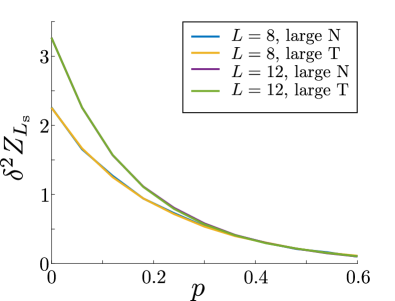
Figure 5: Comparison of trajectory averaging and time averaging for postselected data. The average of the expected variance at the final timestep of 15000 different runs is contrasted with the average of the same at the end of each cycle for a single run over 15000 cycles.

V Data availability

The data supporting the findings of this work are available upon reasonable request.

VI Code availability

The codes implementing the calculations in this work are available upon reasonable request.

VII Author contributions

The authors formulated and developed the project together. K.P. carried out majority of the numerical calculations. The results were analyzed and the manuscript was prepared jointly by the authors.

VIII Acknowledgements

A.G.M. and T.O. acknowledge Jane and Aatos Erkko Foundation for financial support. T.O. also acknowledges the Finnish Research Council project 331094. The authors thank P. Sierant for discussions.

IX Competing Interests

The authors declare no competing interests.

SUPPLEMENTARY INFORMATION

I Charge fluctuations vs entanglement entropy

In this section, we provide analytical results for the entanglement entropy $S_{\text{vN}}$ and the subsystem charge fluctuations $\delta^{2}Z_{L_{s}}$ in $U(1)$-charge conserving random unitary circuits without measurements. As illustrated in Fig. 2c in the main text, the entropy-fluctuation relation is universal and does not depend on the system size or the single-qubit measurement rate. Thus, we can obtain some of the central features of the relation from the vanishing measurement rate $p=0$ case. This analysis essentially determines the relationship between $S_{\text{vN}}$ and $z_{L_{s}}$ in the volume-law regime. For the sake of convenience, we first derive the results for a modified form of the charge operator, $Q_{L}=(L+Z_{L})/2$, which corresponds to labeling qubit charge eigenvalues as $\{0,1\}$ instead of $\{-1,1\}$. The same form is also used for the subsystem charge and the variances will be simply related to each other as $\delta^{2}Q_{L_{s}}=(1/4)\delta^{2}Z_{L_{s}}$.

We first note that the sizes of different sectors of the Hilbert space corresponding to total charges ${\cal Q}_{L}\in(0,\cdots,L)$ are given by

$${\cal N}_{{\cal Q}_{L}}={{L}\choose{{\cal Q}_{L}}}=\frac{L!}{{\cal Q}_{L}!(L-{\cal Q}_{L})!},$$ (5)

which sum to the full Hilbert space size $\sum_{{\cal Q}_{L}=0}^{L}{\cal N}_{{\cal Q}_{L}}=2^{L}$. A generic random state in a charge sector ${\cal Q}_{L}$, which is a superposition of all possible basis states with uniformly distributed random coefficients, can be written as

$$\left|\Psi\right\rangle=\sum_{\{q_{i}\}}^{\prime}c_{q_{1},\cdots,q_{L}}\left|q_{1},\cdots,q_{L}\right\rangle,$$ (6)

with the summation constrained over $q_{i}=0,1$ ($i=1,\cdots,L$) such that $\sum_{i}{q_{i}}={\cal Q}_{L}$. For a random state with a uniformly distributed superposition, the coefficients on average satisfy $|c_{q_{1},\cdots,q_{L}}|^{2}\sim 1/{\cal N}_{{\cal Q}_{L}}$. Considering the charge sector ${\cal Q}_{L}=L/2$ (or $Z_{L}=0$), and half-partitioning the system, the reduced density matrix for each subsystem is block-diagonal, consisting of $L/2$ blocks. Each block corresponds to a different charge sector ${\cal Q}_{L_{s}}\leq L/2$ of the subsystem with a dimension:

$${\cal N}_{{\cal Q}_{L_{s}}}={\frac{L}{2}\choose{{\cal Q}_{L_{s}}}}.$$ (7)

Within any of these blocks, the eigenvalues of the reduced density matrix are approximately equal due to the random nature of the state. By a simple counting argument, the are estimated as

$$p_{{\cal Q}_{L_{s}},i}=\frac{1}{{\cal N}_{{\cal Q}_{L}=\frac{L}{2}}}{\frac{L}{2}\choose{\frac{L}{2}-{\cal Q}_{L_{s}}}},$$ (8)

Applying the rule of sum of the squares of binomial coefficients

$$\sum_{i=0}^{\frac{L}{2}}{L/2\choose{i}}^{2}={L\choose{L/2}},$$ (9)

we can explicitly verify that the condition

$${\rm Tr}(\rho_{s})=\sum_{{\cal Q}_{L_{s}}=0}^{\frac{L}{2}}\sum_{i=1}^{{\cal N}_{{\cal Q}_{L_{s}}}}\>p_{{\cal Q}_{L_{s}},i}=\sum_{{\cal Q}_{L_{s}}=0}^{\frac{L}{2}}{\cal N}_{{\cal Q}_{L_{s}}}\>p_{{\cal Q}_{L_{s}},i}=1,$$ (10)

is satisfied. We can also evaluate the entanglement entropy, whose leading term reads

$${\cal S}_{vN}=-{\rm Tr}(\rho_{s}\ln\rho_{s})\sim\frac{1}{2}\ln{{L}\choose{L/2}}\sim\frac{L}{2}\ln 2,$$ (11)

where terms as ${\cal O}(1)$ or smaller are dropped assuming $L\gg 1$.

To study the subsystem charge fluctuations, we consider the coarse-grained distribution for the subsystem charge which reads

$$P_{{\cal Q}_{L_{s}}}={\cal N}_{{\cal Q}_{L_{s}}}\>p_{{\cal Q}_{L_{s}},i}=\frac{{L/2\choose{{\cal Q}_{L_{s}}}}{L/2\choose{L/2-{\cal Q}_{L_{s}}}}}{{L\choose L/2}}.$$ (12)

This distribution is symmetric under ${\cal Q}_{L_{s}}\leftrightarrow L/2-{\cal Q}_{L_{s}}$ as it is also expected by simply interchanging the two subsystems with each other. Hence, the average charge within subsystems should also satisfy the symmetry which implies $\langle{\cal Q}_{L_{s}}\rangle=L/4$. Through simple algebra and the rule for the sum of squares of binomial coefficients, we find that

$$\langle{\cal Q}_{L_{s}}^{2}\rangle =\sum_{{\cal Q}_{L_{s}}=0}^{L/2}P_{{\cal Q}_{L_{s}}}{\cal Q}_{L_{s}}^{2}=\sum_{{\cal Q}_{L_{s}}=0}^{L/2}\frac{{L/2\choose{{\cal Q}_{L_{s}}}}^{2}}{{L\choose L/2}}{\cal Q}_{L_{s}}^{2}$$

$$=\frac{(\frac{L}{2})^{2}}{{L\choose L/2}}\sum_{{\cal Q}_{L_{s}}=1}^{L/2}{L/2-1\choose{{\cal Q}_{L_{s}}-1}}^{2}$$

$$=\frac{(\frac{L}{2})^{2}}{{L\choose L/2}}{L-2\choose{L/2-1}}=\frac{L^{2}}{16}\frac{L}{L-1}$$ (13)

from which the variance of charge fluctuations are obtained as $\delta^{2}{\cal Q}_{L_{s}}=(1/16)L^{2}/(L-1)$. Consequently, we have $\delta^{2}Z_{L_{s}}=(1/4)L^{2}/(L-1)\sim L/4$ for original charge quantities $Z_{L_{s}}$ used in the main text. Finally, by employing (11), we obtain the fluctuation-entropy relation

$${\cal S}_{vN}=2\ln 2\,\delta^{2}Z_{L_{s}}+\mathcal{O}(1),$$ (14)

which is applicable in the volume-law regime. As seen in Fig. 2c this result is also valid for finite measurement rate $p$ in the volume-law regime $\delta^{2}Z_{L_{s}}>2$. In the subextensive regime $\delta^{2}Z_{L_{s}}<2$, the entropy-fluctuation relation is also linear, but the slope is not captured by a simple analytical formula.

II Properties of the steered ensembles

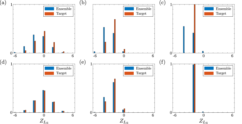
Figure 6: Subsystem charge distribution of the steered ensembles. a-c, Comparison between the expected subsystem $S_{z}$ distribution of a single postselected target trajectory and the measured subsystem spins for 5000 trajectories steered towards this state. Each presents a single target state for an $L=12$ system at $p=0.05,0.145$ and $0.5$ respectively. d-f, Same as above, but using only the data from the $S_{z,\mathrm{tot}}=0$ subset of the (same) steered trajectories.

Here we illustrate the key statistical properties of the steered ensembles. Since the subsystem charge distributions of a single trajectory encodes its entanglement entropy, these distributions are the main focus here.

In Fig. 6(a)-(c), we present the comparison of charge distributions of a single target state $\left|\Psi\right\rangle_{{\bf m}}$ and the corresponding steered ensemble $\rho_{\bf U,m}$. A single target distribution is sensitive to the specific measurement outcomes and, in general, exhibit little symmetry. This indicates that single-trajectory distributions exhibit significant case-to-case fluctuations. The steered charge distributions corresponding to the target are clearly strongly correlated with the target distribution. This correlation is qualitatively better in the volume-law regime.

As Fig. 6(d)-(f) illustrates, the correlation between the target distribution and the steered distribution is dramatically improved by considering only the steered trajectories which end in the same total charge sector $Z_{L}=0$ in which the target trajectory belongs to. In this case the steered distribution is obtained from density matrix $\rho_{\bf U,m}^{Z_{L}=0}$. Deep in the volume-law regime, the match is essentially perfect, but becomes less exact when moving towards the area-law regime.

While the distributions corresponding to individual target trajectories have little symmetry and exhibit strong case-to-case fluctuations, Fig. 8 illustrates how the steered ensemble averaged over many target trajectories are smooth and symmetric. This is just a reflection of the standard postselection problem for nonlinear quantities: it is crucial to first calculate the charge variance from a steered ensemble corresponding to a single target, and only afterwards average over steered ensembles corresponding to different target trajectories.

III Unraveling coherent and incoherent subsystem charge fluctuations

A general counting argument put forward in Ref. [37] suggests that the fluctuations of a conserved extensive charge in a bipartite system exhibit the same spatial scaling with the entanglement entropy. This observation connects entanglement and fluctuations in pure states. Here we explore how the charge fluctuations of a chosen target state $\left|\Psi\right\rangle_{{\bf m}}$ can be extracted from the mixed state density matrix $\rho_{\bf U,m}=\frac{1}{\mathcal{N}_{s}}\sum_{i}\left|\Psi_{i}\right\rangle\left\langle\Psi_{i}\right|$, which is obtained by running the steered dynamics $\mathcal{N}_{s}$ times with the resulting trajectories $\left|\Psi_{i}\right\rangle\equiv\left|\Psi_{{\bf m}^{\prime}_{i}\to{\bf m}}\right\rangle$. Here ${\bf m}^{\prime}_{i}$ denotes the measurement outcomes of $\left|\Psi_{i}\right\rangle$ while ${\bf m}$ denotes the measurement outcomes of the chosen target. For large number of steering realizations, this density matrix approaches to

$$\rho_{\bf U,m}=\sum_{i}p_{i}\left|\Psi_{i}\right\rangle\left\langle\Psi_{i}\right|,$$ (15)

where $p_{i}$ is the probability of trajectory $\left|\Psi\right\rangle_{i}$ in the steered ensemble. The subsystem $U(1)$ charge fluctuations become

$$\delta^{2}Z_{L_{s}}=\langle Z_{L_{s}}^{2}\rangle-\langle Z_{L_{s}}\rangle^{2},$$ (16)

where $Z_{L_{s}}=\sum_{n\in L_{s}}Z_{n}$ and $Z_{n}$ is the Pauli $z$ matrix operating on the $n$th qubit. The first term can be written as

$$\langle Z_{L_{s}}^{2}\rangle=\mathrm{Tr}\left(\rho_{\bf U,m}Z_{L_{s}}^{2}\right)=\mathrm{Tr}\left[\sum_{i}p_{i}\left|\Psi_{i}\right\rangle\left\langle\Psi_{i}\right|Z_{L_{s}}^{2}\right].$$ (17)

The trace is conveniently evaluated in the charge basis $|\mathbf{z}_{L}\rangle$, where $\mathbf{z}_{L}=(\sigma_{1},\sigma_{2}\ldots\sigma_{L})$ with $\sigma_{n}=\pm 1$, and for which $Z_{L_{s}}|\mathbf{z}_{L}\rangle=z_{L_{s}}|\mathbf{z}_{L}\rangle$ with $z_{L_{s}}=\sum_{n\in L_{s}}\sigma_{n}$. Then Eq. (17) becomes

$$\langle Z_{L_{s}}^{2}\rangle=\sum_{\mathbf{z}_{L},i}p_{i}|\langle\mathbf{z}_{L}\left|\Psi_{i}\right\rangle|^{2}z_{L_{s}}^{2}=\sum_{\mathbf{z}_{L}}p_{\mathbf{z}_{L}}z_{L_{s}}^{2},$$ (18)

where

$$p_{\mathbf{z}_{L}}=\sum_{i}p_{i}|\langle\mathbf{z}_{L}\left|\Psi_{i}\right\rangle|^{2}.$$ (19)

In this compact notation, the variance can be expressed as

$$\delta^{2}Z_{L_{s}}=\frac{1}{2}\sum_{\mathbf{z}_{L},\mathbf{z}_{L}^{\prime}}p_{\mathbf{z}_{L}}p_{\mathbf{z}_{L}^{\prime}}(z_{L_{s}}-z_{L_{s}}^{\prime})^{2}.$$ (20)

We can identify two distinct types of terms that contribute to charge fluctuations (20) that we call coherent and incoherent. Each term in (20) involves a product of two probabilities $p_{\mathbf{z}_{L}}p_{\mathbf{z}_{L}^{\prime}}$, which themselves contain contributions from all possible final states $|\psi_{i}(t)\rangle$, as dictated by Eq. (19). The state diagonal terms $i=j$ in the product are the coherent contributions and the off-diagonal terms $i\neq j$ correspond to the incoherent contributions. In a pure state, only coherent fluctuations are present and they encode the entanglement information, as illustrated by the entropy-fluctuation correspondence with the full postselection. The incoherent fluctuations arise from the statistical mixture in $\rho_{\bf U,m}$, and may not reflect the entanglement properties of individual trajectories. In order to probe the entanglement entropy, the incoherent contributions need to be subtracted.

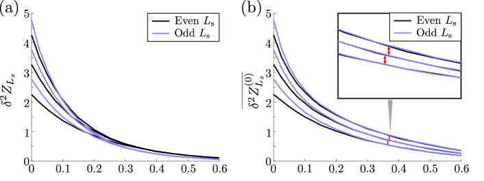
Figure 7: Effects of length parity on the fluctuations. a, Variance as a function of $p$ for postselected data for $L=8,12,16$ (black) and $L=10,14,18$ (red). In the area-law phase, the lines converge to a parity-dependent value that does not otherwise depend on length. b, Variance as a function of $p$ for the steered data with $Z_{L_{\mathrm{s}}}=0$, for the same lengths. The red arrows indicate $2c_{V}(p)$ from Eq. 24.

Let’s consider target trajectories which lie in the total charge sector $Z_{L}=0$. As discussed in Sec. II above, the steering processes break the $U(1)$ charge conservation and the state have a finite weight at $Z_{L}=\pm 2$, $Z_{L}=\pm 4$…$Z_{L}=\pm L$. The density matrix is block diagonal in the $U(1)$ charge sectors $[\rho_{\bf U,m},Z_{L}]=0$, so most of the incoherent processes can be removed by considering only the $Z_{L}=0$ block $\rho_{\bf U,m}^{0}$. This leads to charge fluctuations

$$\delta^{2}Z_{L_{s}}^{(0)}=\frac{1}{2}\sum_{\mathbf{z}_{L},\mathbf{z}_{L}^{\prime}\in\{Z_{L}=0\}}\tilde{p}_{\mathbf{z}_{L}}\tilde{p}_{\mathbf{z}_{L}^{\prime}}(z_{L_{s}}-z_{L_{s}}^{\prime})^{2}.$$ (21)

with normalized probabilities $\tilde{p}_{\mathbf{z}_{L}}=p_{\mathbf{z}_{L}}/(\sum_{{\mathbf{z}_{L}}\in\{Z_{L}=0\}}p_{\mathbf{z}_{L}})$. The projected fluctuations still contains residual incoherent contributions from distinct steering trajectories that end up in the $Z_{L}=0$ sector. As seen in Fig. 6, the projected fluctuations $\delta^{2}Z_{L_{s}}^{(0)}$ already provide an excellent match with the postselected fluctuations deep in the volume-law regime. However, the incoherent contributions from the steering processes, number of which scale as the system size, can be expected to give rise to an addition volume-law fluctuations in the area-law phase. Indeed, the target-trajectory averaged fluctuations

$$\overline{\delta^{2}Z_{L_{s}}^{(0)}}=\frac{1}{N}\sum_{j}\delta^{2}Z_{L_{s}}^{(0)}(j),$$ (22)

where the sum is over $N$ target trajectories $\left|\Psi\right\rangle_{{\bf m}_{j}}$, clearly display additional size-dependent fluctuations even when the target trajectories exhibit area-law fluctuations, as seen in Fig. 4(b).

Fortunately, the coherent and incoherent fluctuations can be easily distinguished by their different system-size dependence.

$$\overline{\delta^{2}Z_{L_{s}}^{(0)}}\sim c_{V}(p)L_{s}+c_{A}(p),$$ (23)

where $c_{A}(p)$ is the area-law coefficient from coherent contribution and $c_{V}(p)$ is the parasitic volume-law coefficient from the incoherent contribution. By comparing the fluctuations of different systems sizes, one can straightforwardly obtain $c_{V}(p)$ and $c_{A}(p)$. As seen in Fig. 7 (b), for any two different subsystem lengths, both being either even or odd, the change in the parasitic term is $\Delta\left(\overline{\delta^{2}Z^{(0)}_{L_{s}}}\right)=c_{V}(p)\Delta L_{s}$. This reflects the volume-law nature of the parasitic term. Fig. 7 (b) also indicates that there is a small offset between the trends for even and odd $L_{s}$, which arises because the last layer of two-qubit unitaries treat the even and odd subsystems differently. This odd-even effect is visible already in the postselected fluctuations seen in Fig. 7(a). The even-odd effect elucidates the expression for $c_{V}(p)$ introduced in the main text in Eq. (3) for successive lengths. Due to the volume-law character of the parasitic term other combinations consistent with the even-odd effect, of the general form

$$c_{V}(p)=\left(\overline{\delta^{2}Z_{L_{s}=2k}^{(0)}}-\overline{\delta^{2}Z_{L_{s}=2k-j}^{(0)}}\right)/(j+1)$$ (24)

with $j$ an odd integer will also work.

Finally, we note that in this charge-conserved case steering will not generate additional fluctuations at system sizes with $L_{s}=1,2$. While the difference in parasitic contributions between adjacent lengths is accurately described above, this causes an additional correction term relevant for small system sizes; taking it into account, the area-law regime parasitic contribution term is expressed as $c_{V}(p)(L_{s}-2)$. The introduction of the small offset $-2c_{V}(p)\sim 0.1$, while having little practical significance – especially for system sizes $L_{s}\gg 2$ – provides an excellent match between the reduced fluctuations $\delta^{2}\widetilde{Z}_{L_{s}}^{(0)}=\overline{\delta^{2}Z_{L_{s}}^{(0)}}-c_{V}(p)\left[L_{s}-2\right]$ and the postselected fluctuation in the area-law regime, as seen in Fig. 4 (c).

IV Estimating the steering overhead

To measure expectation values of observables, it is necessary to prepare multiple copies of a given trajectory $\left|\Psi\right\rangle_{{\bf m}}$ with measurement outcomes ${\bf m}$. In practice, this necessitates running the circuit a number of times which scales exponentially in the system size, a fact which gives rise to the exponentially complex postselection bottleneck in the experimental studies of monitored dynamics. By the virtue of the steering approach discussed in the present work, we can circumvent this bottleneck, as well as the exponential bottleneck associated with the entanglement entropy measurement through state tomography. Crucially, these combined exponential complexities are replaced by a scalable polynomial overhead which we now establish.

For a given target trajectory, the fluctuations are obtained from the steered ensemble by running the steering dynamics $\mathcal{N}_{s}$ times and measuring all the qubits in the charge basis. If the total charge of the full circuit belongs to the sector $Z_{L}=0$, we also consider the measured value for the subsystem charge $Z_{L_{s}}=Z_{i}$. Then, using the values attained for $Z_{i}$ for the successful runs which end up in the total charge $Z_{L}=0$ sector, we can estimate the charge fluctuations of subsystem using the so-called sample variance as

$$\delta^{2}Z_{L_{s}}^{(0)}=\frac{1}{2n^{2}}\sum_{i,j}(Z_{i}-Z_{j})^{2}=\frac{1}{n}\sum_{i}\left(Z_{i}-\langle Z\rangle\right)^{2},$$ (25)

with $\langle Z\rangle$ denoting the sample average of $Z_{i}$ . We see that there are basically two factors to be taken into account to estimate of number of sufficient steering runs:

• the fraction of successful runs (which end up in the $Z_{L}=0$ sector) in all runs $\mathcal{N}_{Z_{L}=0}/\mathcal{N}_{s}$

• the sample-to-sample variations of obtained variances $\delta^{2}Z_{L_{s}}^{(0)}$ with the sample size $\mathcal{N}_{Z_{L}=0}$.

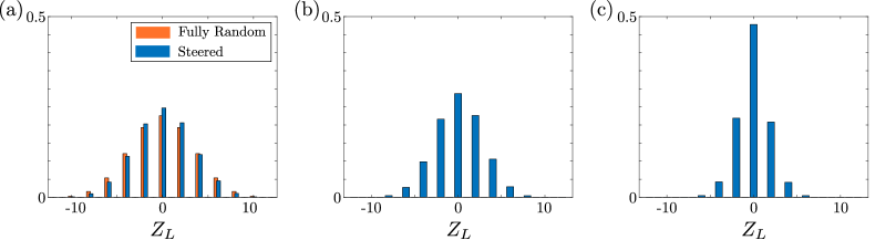
Figure 8: Charge distribution of the steered ensemble. Stationary probability distributions of the total $U(1)$ charge $Z_{L}$ from over 5000 target trajectories with 5000 steered trajectories each for $L=12$ at probabilities a: $p=0.05$, b: $p=0.145$ and c: $p=0.5$ respectively. For comparison, Fig. a also illustrates the fully random distribution where all microstates have equal probability.

To estimate the fraction of successful runs, let us assume that each single qubit measurement event has almost equal probabilities for $0$ and $1$. By running a circuit of length $L$ and depth $T\sim L$ (to reach the steady state), at a measurement rate $p$, on average $m\sim pLT\sim pL^{2}$ qubits are being measured throughout the evolution. Then, total number of different possible steering runs we can have will be ${n}_{\rm s}=2^{m}$, while only

$${n}_{Z_{L}=0}={m\choose\frac{m}{2}}$$ (26)

of them are constraint to have total charge $Z_{L}=0$. Therefore, the success rate of runs is given by

$$\frac{{\cal N}_{Z_{L}=0}}{{\cal N}_{s}}=\frac{n_{Z_{L}=0}}{n_{s}}\sim\sqrt{\frac{2}{\pi m}}\sim\sqrt{\frac{2}{p}}\frac{1}{L}.$$

This is a rather crude approximation based on trajectories for which all measurement outcomes are equally likely, and does not account for steering which drive the trajectories towards the $Z_{L}=0$ sector. As the number of different charge sectors scale as $\sim L$, the $1/L$ scaling is clearly the worst case scenario. In fact, the trajectory-averaged probability distributions in Fig. 8 have Gaussian-type envelope with standard deviation $\sim\sqrt{L}$. This conclusion follows from the comparison to a fully random distribution, where all microstates are equally probable. Due to the enhanced number of states in the low-lying charge sectors of the multiqubit Hilbert space, the random distribution has a standard deviation $\sim\sqrt{L}$. As depicted in Fig. 8(a), the trajectory-averaged steered distribution approaches the fully random case when $p\to 0^{+}$; however, the distribution remains more narrow for all $p$. This indicates that the target-averaged probability of the $Z_{L}=0$ sector scales as $p_{Z=0}\sim\frac{1}{\sqrt{L}}$, hence the mean success fraction per target trajectory also scales as

$$\frac{{\cal N}_{Z_{L}=0}}{{\cal N}_{s}}\sim\frac{1}{\sqrt{L}}.$$ (27)

Next, we estimate the variance of charge fluctuations themselves by considering different samples of fixed size $\mathcal{N}_{Z_{L}=0}$. Ideally, we would like to reduce this “variance of variance” below a small threshold value $\epsilon$. Intuitively, one expects that by increasing the sample size $\mathcal{N}_{Z_{L}=0}$ from which we calculate the subsystem charge fluctuations $\delta^{2}Z_{L_{s}}^{(0)}$, we will have a better estimate with smaller and smaller ${\rm\delta^{2}}\left(\delta^{2}Z_{L_{s}}^{(0)}\right)$. We now show that this intuition is correct and $\delta^{2}Z_{L_{s}}^{(0)}$ decreases with the sample size as $1/\mathcal{N}_{Z_{L}=0}$. In order to determine the variance of variance, we consider sets of different successful steering runs, each consisting of $n=\mathcal{N}_{Z_{L}=0}$ realizations which we label with capital letters to not be mixed with separate steering realizations within each set. Since every set may give a separate charge fluctuations $\delta^{2}_{I}Z$ (from here on, we drop the indices from $\delta^{2}Z_{L_{s}}^{(0)}$ for simplicity), these charge fluctuations for different sets basically introduce a new random variable:

$$Y_{I}=\frac{n\,\delta^{2}_{I}Z}{\delta^{2}_{\infty}Z},$$ (28)

where $\delta^{2}_{\infty}Z$ is the asymptotic value for the charge fluctuations, obtained from a infinitely large set of steering trajectories which end up in the $Z_{L}=0$ charge sector. The variance of variance for subsystem charge is then related to the variance of variable $Y$ (which exhibits sample-to-sample variations between samples with $n=\mathcal{N}_{Z_{L}=0}$ steering realization):

$$\delta^{2}\left(\delta^{2}Z\right)=\delta^{2}\left(\frac{\delta^{2}_{\infty}Z}{n}\,Y\right)=\left(\frac{\delta^{2}_{\infty}Z}{n}\right)^{2}\delta^{2}Y.$$ (29)

We can separate the contribution to this new random variable as

$$Y_{I} =\frac{1}{\delta^{2}_{\infty}Z}\sum_{i\in I}\left(Z_{i}-\langle Z\rangle_{I}\right)^{2}$$

$$=\frac{1}{\delta^{2}_{\infty}Z}\sum_{i\in I}\left(Z_{i}-\langle Z\rangle_{\infty}\right)^{2}-\frac{\left(\langle Z\rangle_{I}-\langle Z\rangle_{\infty}\right)^{2}}{\delta^{2}_{\infty}Z/n}\,,$$ (30)

where we have used the following identity

$$\sum_{i\in I}\left(Z_{i}-\langle Z\rangle_{\infty}\right)^{2}=\sum_{i\in I}\left(Z_{i}-\langle Z\rangle_{I}+\langle Z\rangle_{I}-\langle Z\rangle_{\infty}\right)^{2}$$

$$\qquad=\sum_{i\in I}\left(Z_{i}-\langle Z\rangle_{I}\right)^{2}+n\,\left(\langle Z\rangle_{I}-\langle Z\rangle_{\infty}\right)^{2}.$$ (31)

Now, the first term in the R.H.S. of Eq. (30) can be written as the following sum over separate random variables $\sum_{i}^{n}y_{i}=\sum_{i}^{n}x_{i}^{2}$ where we have substituted $(Z_{i}-\langle Z\rangle_{\infty})/\sqrt{\delta^{2}_{\infty}Z}=x_{i}$. Assuming $Z_{i}$ being derived from a Gaussian statistics, then $x_{i}$ have a simple Gaussian distribution form

$$p(x)=\frac{1}{\sqrt{2\pi}}e^{-x^{2}/2},$$ (32)

as we have already subtracted the mean and then scaled with the standard deviation. Using the central limit theorem, we can see that the same holds for the second term in the R.H.S. of Eq. (30) meaning that $x_{n+1}=(\langle Z\rangle_{I}-\langle Z\rangle_{\infty})/\sqrt{\delta^{2}_{\infty}Z/n}$ has a Gaussian distribution as well. As a result, the statistics of $Y_{I}$ follows from that of a random variable

$$Y=\sum_{i}^{n}y_{i}-y_{n+1}=\sum_{i}^{n}x_{i}^{2}-x_{n+1}^{2}.$$ (33)

The lemma 1 introduced below shows that each $y_{i}$ above follows a $\chi^{2}$-distribution whose variances are $\delta^{2}y_{i}=2$. Now treating different $y_{i}$’s as independent, using Lemma 2 the variance of $Y$ is found to be $2(n-1)$.

Finally, by restoring $n=\mathcal{N}_{Z_{L}=0}$, we find the variance of charge fluctuations is

$$\delta^{2}\left(\delta^{2}Z\right)\sim\frac{2}{\mathcal{N}_{Z_{L}=0}}\,\left(\delta^{2}_{\infty}Z\right)^{2},$$ (34)

which requires $\mathcal{N}_{Z_{L}=0}>\left(\delta^{2}_{\infty}Z\right)^{2}(2/\epsilon)$ in order to have $\delta^{2}\left(\delta^{2}Z\right)<\epsilon$. This gives a lower limit to the number of successful steering runs required to estimate the variance up to an error $\epsilon$. Using the approximate value for the success fraction from Eq. (27), we would need

$$\mathcal{N}_{s}\gtrsim\frac{\sqrt{L}}{\epsilon}\left(\delta^{2}_{\infty}Z\right)^{2}\sim\frac{L^{5/2}}{\epsilon}$$ (35)

which follows from the fact that the variance of the steered ensemble exhibits the volume-law scaling $\delta^{2}_{\infty}Z\propto L$.

IV.1 Lemma 1

The square of a random variable with normalized Gaussian distribution

$$p(x)=\frac{1}{\sqrt{2\pi}}e^{-x^{2}/2}.$$ (36)

is given by $\chi^{2}$-distribution with one degree of freedom.

Proof.—Since $y=x^{2}$, we can have two different branches for $x$ in terms of $y$ which are simply $x_{1}=\sqrt{y}$ and $x_{2}=-\sqrt{y}$ from which we can calculate the probability distribution of $y$ as

$$\tilde{p}(y)=\sum_{i}\left[p(x)|\frac{dx}{dy}|\right]_{x=x_{i}(y)}=\frac{p(\sqrt{y})}{\sqrt{y}}=\frac{e^{-y/2}}{\sqrt{2\pi y}},$$ (37)

which completes the proof. The cumulant generating function for $y=x^{2}$ can be also calculated as below

$${\cal K}_{y}(\theta) =\ln\langle e^{\theta y}\rangle=\ln\int dy\,p(y)e^{\theta y}$$

$$=\ln\int dy\frac{1}{\sqrt{2\pi\,y}}e^{-y/2}e^{\theta y}=\ln\left[(1-2\theta)^{-1/2}\right],$$ (38)

from which we find the mean and variance to be $\langle y\rangle=1$, and $\delta^{2}y=2$, respectively.

IV.2 Lemma 2

The cumulants of sum of independent random variables are given by the sum of the corresponding cumulants for each of those random variables. A special yet interesting case is obviously for the second cumulant as it gives the variance.

Proof.— We show a similar statement is valid for the cumulant generating function and then derive it for the cumulants as they are given by $n$-th derivatives of the cumulant generating function. The cumulant generating function for a random variable $y$ is defined as

$${\cal K}_{y}(\theta)=\ln\langle e^{\theta y}\rangle$$ (39)

If $y$ is sum of independent variables $y_{i}$ as $y=\sum_{i}y_{i}$ then the cumulant generating function for $y$ reads,

$${\cal K}_{y}(\theta) =\ln\langle e^{\theta\sum_{i}y_{i}}\rangle=\ln\langle\prod_{i}e^{\theta y_{i}}\rangle=\ln\left(\prod_{i}\langle e^{\theta y_{i}}\rangle\right)$$

$$=\sum_{i}\ln\langle e^{\theta y_{i}}\rangle=\sum_{i}{\cal K}_{y_{i}}(\theta),$$ (40)

which proves the statement. Note that in the last step of first line we could write the average of product of functions as the product of separate averages, since they are functions of independent random variables.

References

- Skinner et al. [2019] B. Skinner, J. Ruhman, and A. Nahum, Measurement-Induced Phase Transitions in the Dynamics of Entanglement, Phys. Rev. X 9, 031009 (2019).
- Li et al. [2019] Y. Li, X. Chen, and M. P. A. Fisher, Measurement-driven entanglement transition in hybrid quantum circuits, Phys. Rev. B 100, 134306 (2019).
- Fisher et al. [2023] M. P. Fisher, V. Khemani, A. Nahum, and S. Vijay, Random quantum circuits, Annu. Rev. Condens. Matter Phys. 14, 335 (2023).
- Potter and Vasseur [2022] A. C. Potter and R. Vasseur, Entanglement dynamics in hybrid quantum circuits, in Entanglement in Spin Chains: From Theory to Quantum Technology Applications, edited by A. Bayat, S. Bose, and H. Johannesson (Springer International Publishing, Cham, 2022) pp. 211–249.
- Zabalo et al. [2020] A. Zabalo, M. J. Gullans, J. H. Wilson, S. Gopalakrishnan, D. A. Huse, and J. H. Pixley, Critical properties of the measurement-induced transition in random quantum circuits, Phys. Rev. B 101, 060301 (2020).
- Gullans and Huse [2020a] M. J. Gullans and D. A. Huse, Dynamical Purification Phase Transition Induced by Quantum Measurements, Phys. Rev. X 10, 041020 (2020a).
- Szyniszewski et al. [2019a] M. Szyniszewski, A. Romito, and H. Schomerus, Entanglement transition from variable-strength weak measurements, Phys. Rev. B 100, 064204 (2019a).
- Bharti et al. [2022] K. Bharti, A. Cervera-Lierta, T. H. Kyaw, T. Haug, S. Alperin-Lea, A. Anand, M. Degroote, H. Heimonen, J. S. Kottmann, T. Menke, W.-K. Mok, S. Sim, L.-C. Kwek, and A. Aspuru-Guzik, Noisy intermediate-scale quantum algorithms, Rev. Mod. Phys. 94, 015004 (2022).
- Li et al. [2018] Y. Li, X. Chen, and M. P. A. Fisher, Quantum Zeno effect and the many-body entanglement transition, Phys. Rev. B 98, 205136 (2018).
- Cao et al. [2019] X. Cao, A. Tilloy, and A. D. Luca, Entanglement in a fermion chain under continuous monitoring, SciPost Phys. 7, 24 (2019).
- Szyniszewski et al. [2019b] M. Szyniszewski, A. Romito, and H. Schomerus, Entanglement transition from variable-strength weak measurements, Phys. Rev. B 100, 064204 (2019b).
- Ippoliti et al. [2021] M. Ippoliti, M. J. Gullans, S. Gopalakrishnan, D. A. Huse, and V. Khemani, Entanglement phase transitions in measurement-only dynamics, Phys. Rev. X 11, 011030 (2021).
- Noel et al. [2022] C. Noel, P. Niroula, D. Zhu, A. Risinger, L. Egan, D. Biswas, M. Cetina, A. V. Gorshkov, M. J. Gullans, D. A. Huse, and C. Monroe, Measurement-induced quantum phases realized in a trapped-ion quantum computer, Nature Physics 18, 760 (2022).
- Hoke et al., (2023) [Google Quantum AI and Collaborators] J. C. Hoke et al., (Google Quantum AI and Collaborators), Measurement-induced entanglement and teleportation on a noisy quantum processor, Nature 622, 481 (2023).
- Koh et al. [2023] J. M. Koh, S.-N. Sun, M. Motta, and A. J. Minnich, Measurement-induced entanglement phase transition on a superconducting quantum processor with mid-circuit readout, Nature Physics 19, 1314 (2023).
- Kamakari et al. [2024] H. Kamakari, J. Sun, Y. Li, J. J. Thio, T. P. Gujarati, M. P. A. Fisher, M. Motta, and A. J. Minnich, Experimental demonstration of scalable cross-entropy benchmarking to detect measurement-induced phase transitions on a superconducting quantum processor (2024), arXiv:2403.00938 [quant-ph] .
- Li et al. [2023] Y. Li, Y. Zou, P. Glorioso, E. Altman, and M. P. A. Fisher, Cross entropy benchmark for measurement-induced phase transitions, Phys. Rev. Lett. 130, 220404 (2023).
- Gullans and Huse [2020b] M. J. Gullans and D. A. Huse, Scalable Probes of Measurement-Induced Criticality, Phys. Rev. Lett. 125, 070606 (2020b).
- Ippoliti and Khemani [2021] M. Ippoliti and V. Khemani, Postselection-free entanglement dynamics via spacetime duality, Phys. Rev. Lett. 126, 060501 (2021).
- Dehghani et al. [2023] H. Dehghani, A. Lavasani, M. Hafezi, and M. J. Gullans, Neural-network decoders for measurement induced phase transitions, Nature Communications 14, 2918 (2023).
- Garratt et al. [2023] S. J. Garratt, Z. Weinstein, and E. Altman, Measurements conspire nonlocally to restructure critical quantum states, Phys. Rev. X 13, 021026 (2023).
- McGinley [2024] M. McGinley, Postselection-free learning of measurement-induced quantum dynamics, PRX Quantum 5, 020347 (2024).
- Buchhold et al. [2022] M. Buchhold, T. Mueller, and S. Diehl, Revealing measurement-induced phase transitions by pre-selection, arXiv:2208.10506 (2022).
- Sierant and Turkeshi [2023a] P. Sierant and X. Turkeshi, Entanglement and absorbing state transitions in (d+1)-dimensional stabilizer circuits, Acta Phys. Pol., A 144, 474 (2023a).
- Moghaddam et al. [2023] A. G. Moghaddam, K. Pöyhönen, and T. Ojanen, Exponential shortcut to measurement-induced entanglement phase transitions, Phys. Rev. Lett. 131, 020401 (2023).
- Oshima and Fuji [2023] H. Oshima and Y. Fuji, Charge fluctuation and charge-resolved entanglement in a monitored quantum circuit with symmetry, Phys. Rev. B 107, 014308 (2023).
- Note [1] Note that the index for steered states has been dropped for brevity.
- Iqbal et al. [2023] M. Iqbal, N. Tantivasadakarn, T. M. Gatterman, J. A. Gerber, K. Gilmore, D. Gresh, A. Hankin, N. Hewitt, C. V. Horst, M. Matheny, T. Mengle, B. Neyenhuis, A. Vishwanath, M. Foss-Feig, R. Verresen, and H. Dreyer, Topological order from measurements and feed-forward on a trapped ion quantum computer, arXiv:2302.01917 (2023).
- Sivak et al. [2023] V. Sivak, A. Eickbusch, B. Royer, S. Singh, I. Tsioutsios, S. Ganjam, A. Miano, B. Brock, A. Ding, L. Frunzio, et al., Real-time quantum error correction beyond break-even, Nature 616, 50 (2023).
- Acharya et al., (2023) [Google Quantum AI and Collaborators] R. Acharya et al., (Google Quantum AI and Collaborators), Suppressing quantum errors by scaling a surface code logical qubit, Nature 614, 676 (2023).
- Terhal [2015] B. M. Terhal, Quantum error correction for quantum memories, Rev. Mod. Phys. 87, 307 (2015).
- Friedman et al. [2023] A. J. Friedman, O. Hart, and R. Nandkishore, Measurement-induced phases of matter require feedback, PRX Quantum 4, 040309 (2023).
- Ravindranath et al. [2023] V. Ravindranath, Y. Han, Z.-C. Yang, and X. Chen, Entanglement steering in adaptive circuits with feedback, Phys. Rev. B 108, L041103 (2023).
- Sierant and Turkeshi [2023b] P. Sierant and X. Turkeshi, Controlling entanglement at absorbing state phase transitions in random circuits, Phys. Rev. Lett. 130, 120402 (2023b).
- O’Dea et al. [2024] N. O’Dea, A. Morningstar, S. Gopalakrishnan, and V. Khemani, Entanglement and absorbing-state transitions in interactive quantum dynamics, Phys. Rev. B 109, L020304 (2024).
- Agrawal et al. [2022] U. Agrawal, A. Zabalo, K. Chen, J. H. Wilson, A. C. Potter, J. H. Pixley, S. Gopalakrishnan, and R. Vasseur, Entanglement and Charge-Sharpening Transitions in U(1) Symmetric Monitored Quantum Circuits, Phys. Rev. X 12, 041002 (2022).
- Pöyhönen et al. [2022] K. Pöyhönen, A. G. Moghaddam, and T. Ojanen, Many-body entanglement and topology from uncertainties and measurement-induced modes, Phys. Rev. Res. 4, 023200 (2022).
- Note [2] We note that slightly more precise expression for the sample variance is given by as in a sample of size , by calculating we are left with independent degrees of freedom.