Unveiling the Unknown: Conditional Evidence Decoupling for Unknown Rejection

Abstract

In this paper, we focus on training an open-set object detector under the condition of scarce training samples, which should distinguish the known and unknown categories. Under this challenging scenario, the decision boundaries of unknowns are difficult to learn and often ambiguous. To mitigate this issue, we develop a novel open-set object detection framework, which delves into conditional evidence decoupling for the unknown rejection. Specifically, we select pseudo-unknown samples by leveraging the discrepancy in attribution gradients between known and unknown classes, alleviating the inadequate unknown distribution coverage of training data. Subsequently, we propose a Conditional Evidence Decoupling Loss (CEDL) based on Evidential Deep Learning (EDL) theory, which decouples known and unknown properties in pseudo-unknown samples to learn distinct knowledge, enhancing separability between knowns and unknowns. Additionally, we propose an Abnormality Calibration Loss (ACL), which serves as a regularization term to adjust the output probability distribution, establishing robust decision boundaries for the unknown rejection. Our method has achieved the superiority performance over previous state-of-the-art approaches, improving the mean recall of unknown class by 7.24% across all shots in VOC10-5-5 dataset settings and 1.38% in VOC-COCO dataset settings. The code is available via https://github.com/zjzwzw/CED-FOOD.

1 Introduction

Object detection [33, 10, 3, 19, 32, 46] has made significant achievements in the field of deep learning, facilitating downstream detection tasks by training a large number of samples. This premise relies on the abundant closed-set training data, where test and training sets share the same categories. However, in real-world scenarios such as safe autonomous driving, the available annotation data is limited and there are numerous unlabeled unknown objects, which could cause serious safety accidents. Therefore, training detectors to both recognize the known and reject the unknown is crucial for the deployment of real-world applications.

Recently, the Few-shot Open-set Object Detection (FOOD) is gaining more attention, alleviating traditional closed-set detectors’ limitations by addressing the challenge of unknown rejection. Unlike closed-set frameworks, few-shot open-set frameworks break the conventional constraint of identical class labels in training and testing sets, enabling the detection of known classes and the rejection of unknown classes with training solely on few-shot closed-set data. This task poses considerable challenges due to insufficient training data and the absence of labels for unknown objects, leading to a weak generalization of unknown discovery and resulting in a low recall rate.

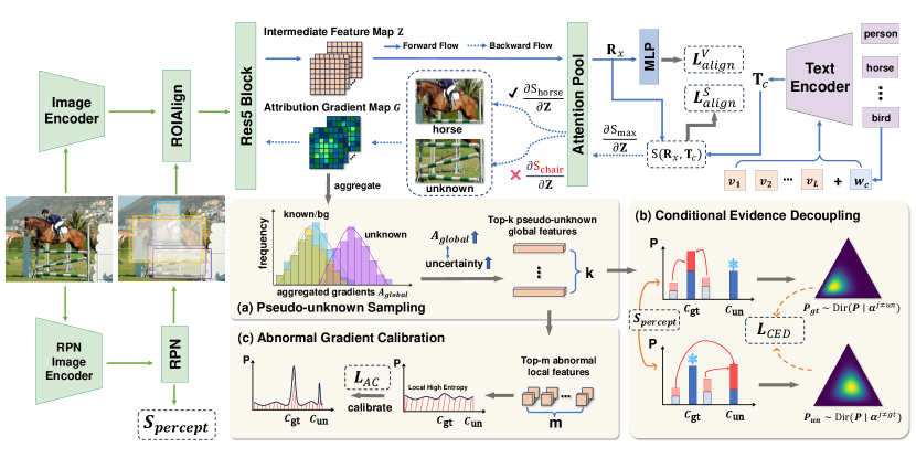
Figure 1: The overview architecture of our method. Our method is a two-stage detector with (a) Gradient-based Attribution For Pseudo-unknown Sampling, (b) Conditional Evidence Decoupling For Unknown Optimization, (c) Abnormal Gradient Calibration For Robust Decision Boundary. We first derive attribution gradients $\boldsymbol{G}$ from the maximum matching scores $\text{S}_{\text{max}}$ in the semantic space applied to intermediate visual features $\mathbf{Z}$, and select pseudo-unknown samples ranked by global aggregation of these gradients. For these pseudo-unknown samples, we decouple training in the form of Evidential Deep Learning (EDL) with object perception scores, denoted as $\boldsymbol{L}_{CED}$. Simultaneously, we perform local aggregation of gradients to filter out anomalies and calibrate the distribution of local features, denoted as $\boldsymbol{L}_{AC}$.

Previous FOOD methods have utilized weight sparsification [40] or moving weight averages [41] to facilitate generalization for unknown classes in few-shot open-set scenarios. However, the detector is prone to overfit the known classes due to insufficient training data, resulting in ambiguous decision boundaries between known and unknown classes. This ambiguity often leads to misclassification of unknown classes as known ones with a high confidence score. Therefore, establishing discriminative decision boundaries in the representation space is crucial to enhance the identification of unknown classes. Drawing inspiration from the gradient-based attribution method [5] for uncertainty estimation, we mine pseudo-unknown samples with the high uncertainty from the known distribution. However, these pseudo samples often couple known and unknown features, which cannot fit the real unknown distribution, causing ambiguous decision boundaries for the unknown rejection. To mitigate this problem, we decouple them conditionally based on the evidence theory.

In this paper, we first exploit the difference in matching scores on the attribution gradient to select pseudo-unknown samples. To construct the decision boundaries, the proposed Conditional Evidence Decoupling Loss (CEDL) decouples known and unknown properties by leveraging object perception scores, which are generated by a separately trained region proposal network (RPN). This approach is derived from the uncertainty mining property of Evidential Deep Learning while removing the evidence influence of the ground truth class. Subsequently, the proposed Abnormalty Calibration Loss (ACL) adjusts the output probability distribution based on an entropy-based regularization term to strengthen the decision boundaries. Furthermore, we incorporate prompt learning augmented with visual contrastive learning, which can leverage rich semantics to separate visually similar objects better. This approach facilitates intra-class compactness and inter-class separability in both semantic and visual perspectives. Experimental results demonstrate the superiority of our method on both known and unknown class metrics. We summarize our main contributions as follows:

• To the best of our knowledge, we are the first work to employ prompt learning augmented by visual contrastive learning for the unknown rejection, which promotes the separation of class features from both visual and semantic perspectives.

• To mine the pseudo-unknown samples, we develop the interpretative uncertainty exhibited by attribution gradients, which discover the difference between known and unknown classes in gradient space.

• We propose a novel Conditional Evidence Decoupling Loss (CEDL) based on Evidential Deep Learning, complemented by the Abnormality Calibration Loss (ACL) for optimization, which could regularize the model to form a compact unknown decision boundary.

2 Related Work

Few-Shot Open-Set Recognition / Object Detection. In open-world scenarios, Few-Shot Open-Set Recognition (FSOSR) [22, 14, 48, 2, 28] aims to train models on image-level representations using limited training data, facilitating the recognition of known classes and the rejection of unknown ones. Compared with FSOSR, few-shot open-set object detection (FOOD) necessitates the detection of all known and unknown objects within an image. Su et al. [40] initially established a benchmark for the FOOD task, which involved randomly sparsifying parts of the normalized weights to reduce co-adaptability among classes. To enhance generalization for unknown classes, Su et al. [41] proposed a Hilbert-Schmidt Independence Criterion (HSIC) based moving weight averaging technique to regulate the updating of model parameters.

Out-Of-Distribution Detection. The objective of out-of-distribution (OOD) detection is to enable the model to differentiate between in-distribution (ID) and OOD samples while preserving its accuracy in classifying ID samples. OOD methods can be divided into two types: training-auxiliary [8, 45, 18, 27, 29] and post-hoc [23, 42, 43, 26, 7, 47, 11, 1, 5, 24] methods. Training-auxiliary methods such as Du et al. [8] enhanced energy scores by synthesizing virtual anomalies. Post-hoc methods such as GAIA [5] inspected the abnormalities in attribution gradients and then aggregated them for OOD detection.

Prompt Learning. By converting hard prompts into continuously learnable prompt vectors, prompt learning can quickly fine-tune the model to adapt to downstream tasks in a parameter-efficient manner, such as CoOp [56] and CoCoOp [55]. While many studies [52, 26, 27, 49, 38] have adopted this method for out-of-distribution (OOD) detection, few have applied prompt learning to object detection in open-world settings.

3 Method

Our method is a prompt-based method that includes: a novel gradient-based attribution approach for pseudo-unknown samples mining, a conditional evidence decoupling loss for unknown optimization, and an abnormal gradient calibration loss for robust unknown decision boundary. An overview of our method is shown in Fig. 1.

3.1 Preliminary

We formalize the FOOD task based on previous research [40, 41]. The object detection dataset $D$ is divided into training data $D_{tr}$ and testing data $D_{te}$. The training set $D_{tr}$ includes $K$ known classes denoted as $C_{K}=C_{B}\cup C_{N}$, where $C_{B}$ represents $B$ base known classes, and $C_{N}$ represents $N$ novel known classes, each with $M$-shot support samples. In addition to $K$ known classes, the test set contains unknown classes $C_{U}$ that do not overlap with the known class labels. As it is impractical to enumerate infinite unknown classes, we denote the unknown classes as $C_{U}=\{K+1\}$. Furthermore, the background class $C_{BG}=\{K+2\}$ is non-negligible. Thus, the FOOD task can be summarized as training a detector with a class-imbalanced training dataset, which could accurately classify the known classes $C_{K}$, reject all unknown classes $C_{U}$, and distinguish between foreground and background according to $C_{BG}$.

Semantic-wise. Previous approaches in Few-Shot Open-Set Object Detection (FOOD) primarily utilized visual knowledge in their classifiers, neglecting potential semantic confusion [34] due to the absence of semantic information. To mitigate this problem, we adopt an image-text alignment training approach (e.g., CLIP [31]), based on the prompt learning method CoOp [56], where prompt templates’ context words (e.g., “a photo of a”) are replaced with continuously learnable parameters, denoted as $\mathbf{t}_{c}=\left\{\boldsymbol{v}_{1},\boldsymbol{v}_{2},\ldots,\boldsymbol{v}_{L},\boldsymbol{w}_{c}\right\}$. Here, $\boldsymbol{v}_{1},\boldsymbol{v}_{2},\ldots,\boldsymbol{v}_{L}$ represent learnable vectors with the same dimension, $L$ denotes the length of context words, and $\boldsymbol{w}_{c}$ represents the word embedding of class $c$. The text encoder processes the prompt vector $\mathbf{t}_{c}$ to output the textual feature vector $\mathbf{T}_{c}$, forming image-text training pairs $\left(\mathbf{R}_{i},\mathbf{T}_{j}\right)$ with visual feature $\mathbf{R}_{i}$ from $N$ region proposals. The semantic alignment loss is defined as:

$${\boldsymbol{L}_{align}^{S}=-\frac{1}{N}\sum_{i=1}^{N}\sum_{j=1}^{K+2}{y}_{ij}\log\frac{\exp\left(\textup{S}\left(\mathbf{R}_{i},\mathbf{T}_{j}\right)/\tau\right)}{\sum_{c=1}^{K}\exp\left(\left(\textup{S}\left(\mathbf{R}_{i},\mathbf{T}_{c}\right)\right)/\tau\right)}},$$ (1)

where $\textup{S}\left(\cdot,\cdot\right)$ represents the cosine similarity and $\tau$ denotes the temperature parameter, ${y}_{ij}$ is an indicator (0 or 1) of sample $i$ belonging to category $j$ in the ground truth label.

Visual-wise. Semantic alignment only forms semantic clusters through the interaction of text and image representations, ignoring the potential relationship between different visual representations, which can improve downstream task performance [44, 12, 16]. Therefore, we propose to augment semantic contrastive learning with visual representation. We map the visual features $\mathbf{R}$ through an MLP to a latent space, generating 128-dimensional latent embeddings $\mathbf{z}$. Following Han et al. [12], we implement enqueue/dequeue operations based on the memory bank and regularize the model with the following visual alignment loss:

$${\boldsymbol{L}_{align}^{V}=\frac{1}{N}\sum_{i=1}^{N}\boldsymbol{L}_{align}^{V}\left(\mathbf{z}_{i}\right)},$$ (2)

$${\boldsymbol{L}_{align}^{V}\left(\mathbf{z}_{i}\right)=\frac{1}{\left|Q\left(\mathbf{c}_{i}\right)\right|}\sum_{\mathbf{z}_{j}\in Q\left(\mathbf{c}_{i}\right)}\log\frac{\exp\left(\mathbf{z}_{i}\cdot\mathbf{z}_{j}/\varepsilon\right)}{\sum_{\mathbf{z}_{k}\in Q\backslash{Q}_{\mathbf{c}_{i}}}\exp\left(\mathbf{z}_{i}\cdot\mathbf{z}_{k}/\varepsilon\right)}},$$ (3)

where $\mathbf{c}_{i}$ is the class label for the $i$-the proposal, $\varepsilon$ is a hyperparameter, and $Q\left(\mathbf{c}_{i}\right)$ represents the embedding queue for class $\mathbf{c}_{i}$. This loss can assist the alignment in the semantic space from a visual perspective, which can enhance intra-class compactness and inter-class separation, thereby leaving more space for unknown classes.

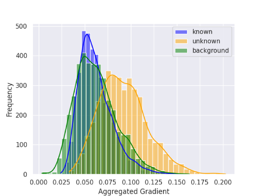
(a) VOC07+12trainval

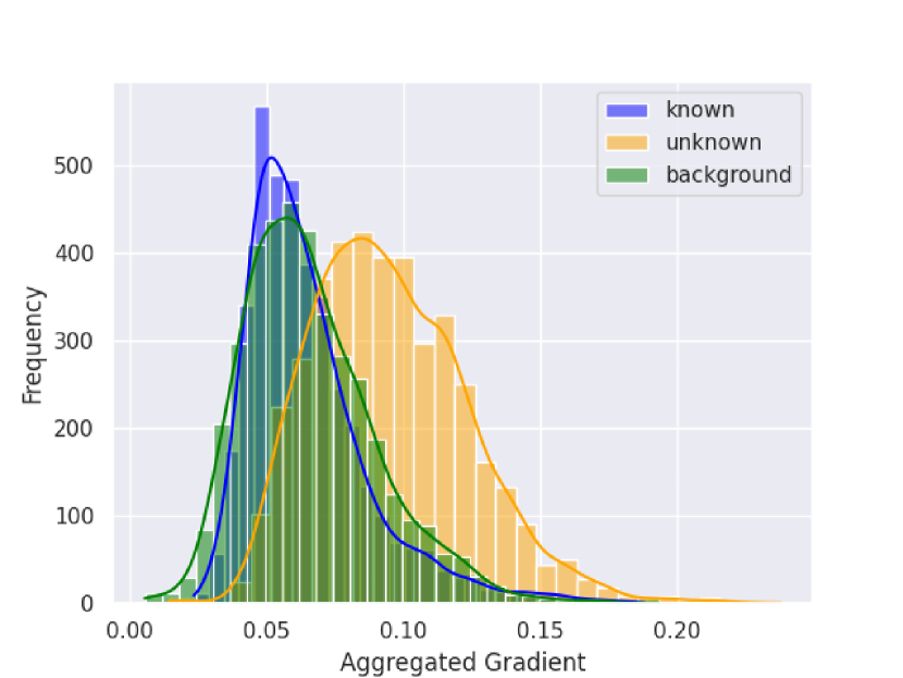
(b) VOC07test

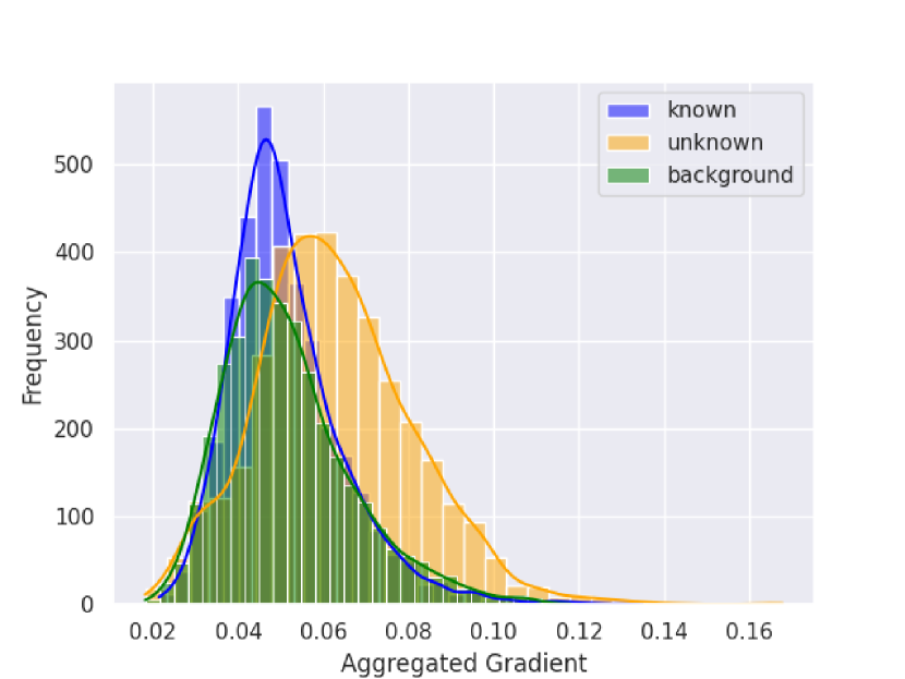
(c) COCO2017val

Figure 2: The distribution of global aggregation attribution gradient for known, background, and unknown classes. We select proposals generated from a random selection of 500 images in both the VOC10-5-5 base training and testing sets, and the VOC-COCO testing set as illustrated in Sec. 4.1. Note that the VOC-COCO training set is only labeled with base classes, thus we exclude it.

3.2 Gradient-based Attribution For Pseudo-unknown Sampling

Due to the inadequate unknown distribution coverage of training data, it is difficult to establish clear unknown decision boundaries. To tackle the above issue, we select a subset of known proposals as pseudo-unknown samples, which may exhibit features of unknown classes. Inspired by the gradient-based attribution method, which was first introduced in the sensitivity analysis (SA) [39], it evaluates the sensitivity of a particular input feature on the final prediction output for visual interpretability [35, 4]. In recent work, Chen et al. [5] found that the aggregated attribution gradients can establish a discriminative separation between ID and OOD to improve out-of-distribution detection. We leverage this property to estimate uncertainty and propose a novel method to mine high-uncertainty pseudo-unknown samples, which are then employed to construct unknown decision boundaries. This can also be expressed as the credibility of visual features described by text. Specifically, we take the intermediate feature layer $\mathbf{Z}$ (in Fig. 1) as the target layer. For a given proposal feature $\mathbf{R}_{x}$, we obtain the attribution gradient at $\text{Z}_{ij}^{k}$ corresponding to the maximum text-image matching score:

$${{G}_{ij}^{k}=\frac{\partial\max_{c=1\ldots K}\textup{S}\left(\mathbf{R}_{x},\mathbf{T}_{c}\right)}{\partial\text{Z}_{ij}^{k}}},$$ (4)

where $i$, $j$, and $k$ represent the indices of height, width, and channel, respectively. We can obtain the attribution gradient map $\boldsymbol{G}$ corresponding to different proposals. Consequently, we perform global aggregation of attribution gradients as follows:

$${A_{global}=\frac{1}{C}\sum_{k}^{C}\left(\sum_{i}^{H}\sum_{j}^{W}\gamma_{ij}^{k}\right)\cdot\left(\sum_{i}^{H}\sum_{j}^{W}\left|G_{ij}^{k}\right|\right)},$$ (5)

where $\gamma_{ij}^{k}$ is an indicator function such that $\gamma_{ij}^{k}=1$ if $G_{ij}^{k}\neq 0$ and $\gamma_{ij}^{k}=0$ if $G_{ij}^{k}=0$, and $|\cdot|$ denotes the absolute function, resulting in a scalar aggregated outcome. The Sec. A of the supplementary materials shows the rationale behind the design of $A_{global}$. We then analyze the distributions of $A_{global}$ for known, background, and unknown classes with all labels available, identifying distinct distribution patterns, as shown in Fig. 2. Under the premise of having only known class labels, a higher $A_{global}$ aligns more closely with the distribution characteristic of unknown classes, suggesting a higher likelihood of containing unknown information. Therefore, we select the proposals corresponding to the top-$k$ highest $A_{global}$ from the foreground and background proposals as pseudo-unknown samples with sampling ratio $S_{fg:bg}$.

3.3 Conditional Evidence Decoupling For Unknown Optimization

Object perception score. We utilize the score output by the Region Proposal Network (RPN) as a decoupling weight factor, indicating the presence of an object. To alleviate the issue of traditional RPNs falsely being class-agnostic (overfitting training categories) [51, 30, 17, 57, 34], we train an RPN with a separate backbone and add a parallel branch to compute the centerness score [46], as shown in Fig. 6, which provides a more robust localization ability from object position and shape. The final score is calculated as the geometric mean of the original objectness score $S_{obj}$ and the centerness score $S_{center}$, which is called the object perception score:

$${S_{percept}=\sqrt{S_{obj}\cdot S_{center}}}.$$ (6)

Evidential deep learning based conditional evidence decoupling. For FOOD, the unknown objects are easily misclassified into known ones with a high confidence score, which could be attributed to its coupling of known and unknown information. We model the relationship between known and unknown classes based on conditional evidence, aiming to decouple and learn distinct information from the pseudo-unknown sample, resulting in a discriminative decision boundary between known and unknown classes. Specifically, we employ Evidential Deep Learning (EDL) [36] based on the evidence framework of Dempster-Shafer Theory (DST) [37] and the subjective logic (SL) [15] to estimate uncertainty. By assuming that the network’s output probabilities $\boldsymbol{P}$ follow a Dirichlet distribution, denoted as $\boldsymbol{P}\sim\operatorname{Dir}\left(\boldsymbol{P}\mid\boldsymbol{\alpha}\right)$, EDL constructs distribution of distributions for uncertainty modeling. This approach could alleviate the overfitting issues caused by the point estimation of the original softmax probability outputs. Drawing on the DST and SL theory, for a classifier with $K+2$ classes, we denote $\exp(l_{i}^{j})$ as the evidence output for the $j$-th class from the $i$-th proposal, where $l_{i}^{j}=\textup{S}\left(\mathbf{R}_{i},\mathbf{T}_{j}\right)/\tau$. Consequently, this allows us to derive the parameters for the Dirichlet distribution:

$${\alpha_{i}^{j}=\exp(l_{i}^{j})+1}.$$ (7)

To extract distinct knowledge from identical features, we optimize evidence for known and unknown classes separately. In this case, the contradictory evidence of decoupled classes simultaneously serves as a negative term, which could lead to a non-convergence phenomenon. To mitigate this interference, we eliminate the evidence of the ground-truth class while optimizing for the unknown class, and conversely, while optimizing for the known class, the evidence of the unknown class is removed. We formalize this as a conditional EDL loss in the following form:

$${\boldsymbol{L}_{i}^{un}=\psi\left(\sum_{j=1,j\neq gt}^{K+2}\alpha_{i}^{j}\right)-\psi\left(\alpha_{i}^{un}\right)},$$ (8)

$${\boldsymbol{L}_{i}^{gt}=\psi\left(\sum_{j=1,j\neq un}^{K+2}\alpha_{i}^{j}\right)-\psi\left(\alpha_{i}^{gt}\right)},$$ (9)

where $\psi(\cdot)$ represents the digamma function, $\boldsymbol{L}^{un}$ and $\boldsymbol{L}^{gt}$ optimize the evidence for the known and unknown classes, respectively. Subsequently, we use the object perception scores mentioned previously as weight factors to balance the optimization between known and unknown classes. For foreground proposals and background proposals, we employ an oppositional balancing approach because, intuitively, a higher score in foreground proposals indicates more known information, thereby increasing the weight for optimizing known classes. Conversely, a higher score in background proposals suggests more unknown information, thus increasing the weight for optimizing unknown classes. Consequently, we derive the following foreground and background conditional evidence decoupling losses:

$${\boldsymbol{L}_{CED}^{fg}=\frac{1}{N}\sum_{i=1}^{N}\left(1-{S_{percept}}_{i}\right)\cdot L_{i}^{un}+{S_{percept}}_{i}\cdot L_{i}^{gt}},$$ (10)

$${\boldsymbol{L}_{CED}^{bg}=\frac{1}{N}\sum_{i=1}^{N}{S_{percept}}_{i}\cdot L_{i}^{un}+\left(1-{S_{percept}}_{i}\right)\cdot L_{i}^{gt}},$$ (11)

thus, the final loss expression is as follows:

$${\boldsymbol{L}_{CED}=\boldsymbol{L}_{CED}^{fg}+\boldsymbol{L}_{CED}^{bg}}.$$ (12)

By optimizing the above loss function, the detector can learn discriminative knowledge from pseudo-unknown samples, ultimately establishing clear decision boundaries between known and unknown classes.

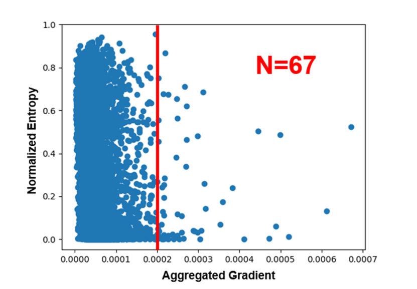
(a) known scatter

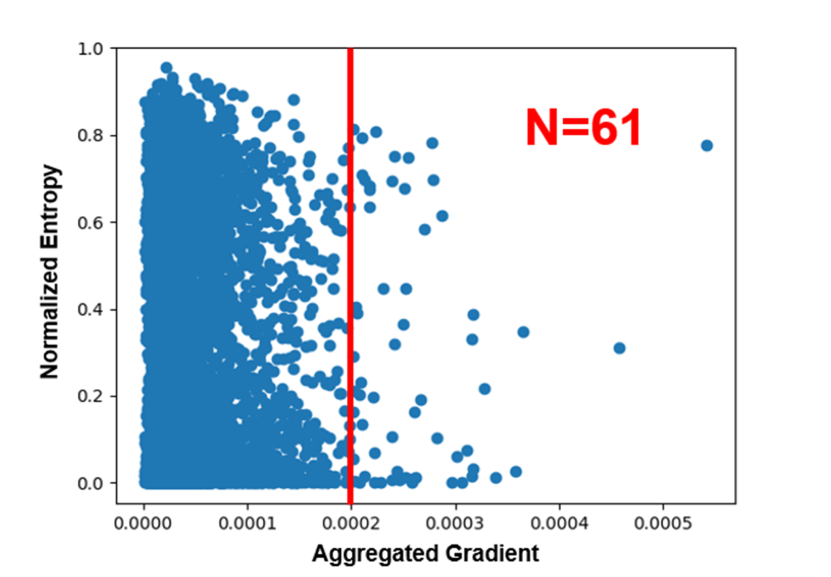
(b) background sactter

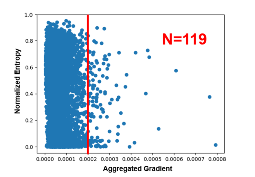
(c) unknown scatter

Figure 3: The scatter plots of known, background, and unknown classes on the VOC07+12trainval dataset. Each point represents a specific local feature $\mathbf{Z}_{xy}$ from intermediate output $\mathbf{Z}$. We select 300 proposals for each plot, unknown class proposals exhibit twice as many local aggregated gradient outliers (thresholded at 0.0002) compared to known and background classes.

3.4 Abnormal Gradient Calibration For Robust Decision Boundary

The final global feature R could be obtained from the intermediate feature Z through an attention pooling operation, where each position $(x,y)$ stands for a local feature $\mathbf{Z}_{xy}$. By employing Eq. 12, the detector can distinguish known and unknown classes using global features. However, certain local anomalous features $\mathbf{Z}_{xy}$ still pose a disruption to the decision-making process of the model. Therefore, we delve into the reasons for the differences in global attribution gradient distributions by aggregating local attribution gradients. We observe that, compared to known and background classes, unknown classes exhibit a greater number of outliers in locally aggregated attribution gradients, as shown in Fig. 3. For the attribution gradient map $G$, we performed aggregation along the channel dimension, resulting in local aggregation results as follows:

$${A_{local}=\frac{1}{C}\sum_{k}^{C}\left|G_{xy}^{k}\right|},$$ (13)

for each local position $(x,y)$, $A_{local}$ is a scalar, $C$ is the total number of channels. We believe that the outlier gradients correspond to local features with high uncertainty, which confuses the global feature discrimination between known and unknown classes. Consequently, we aim to recalibrate the output probability distribution of these local features, reducing the logits for non-ground-truth outputs to diminish over-confidence predictions, and leveraging the normalized entropy to learn about unknown information. Specifically, we first project the pseudo-unknown local features $\mathbf{Z}_{xy}$ into the image-text joint space: $Proj_{v\rightarrow t}(\mathbf{W}_{value}\cdot\mathbf{Z}_{xy})$, where $\mathbf{W}_{value}$ represents the value projection within the attention pool, while $Proj(\cdot)$ denotes the projection from visual to textual space. Similarly, the match scores between local and textual features are computed to obtain the local output logits $l{{}^{\prime}}$. These logits are then adjusted using the following abnormality calibration loss to recalibrate the local output distribution:

$${\boldsymbol{L}_{AC}=-\frac{1}{M}\sum_{i}^{M}\left(\sum_{j=1,j\neq gt}^{K}\log\frac{\exp(-l{{}^{\prime}}_{i}^{j})}{1+\exp(-l{{}^{\prime}}_{i}^{j})}+H_{norm}(\boldsymbol{p}{{}^{\prime}})\cdot\log\frac{1}{1+\exp(-l{{}^{\prime}}_{i}^{un})}\right)},$$ (14)

where $H_{norm}(\boldsymbol{p})=-{\textstyle\sum_{c}p{{}^{\prime}}_{c}\log{p{{}^{\prime}}_{c}}}/\log(K)$ represents the normalized entropy, indicating the uncertainty of the original probability distribution and serving as a weighting factor to constrain the learning of the unknown class. For each pseudo-unknown sample, we select the local features corresponding to the top-$m$ highest $A_{local}$ to recalibrate the output probability distribution, which eliminates the confusion between known and unknown classes caused by local attention, thereby establishing a more robust decision boundary for unknown rejection.

3.5 Overall Optimization

We adopt a two-stage fine-tuning strategy [50] to train the few-shot open-set detector, for the base training stage:

$${\boldsymbol{L}_{base}=\boldsymbol{L}_{reg}+\boldsymbol{L}_{align}^{S}+\boldsymbol{L}_{align}^{V}},$$ (15)

and for the few-shot fine-tuning stage:

$${\boldsymbol{L}_{novel}=\boldsymbol{L}_{reg}+\boldsymbol{L}_{align}^{S}+\boldsymbol{L}_{align}^{V}+\lambda_{t}(\boldsymbol{L}_{CED}+\beta\boldsymbol{L}_{AC})},$$ (16)

where $\boldsymbol{L}_{reg}$ is smooth L1 loss for box regression, $\beta$ is a hyperparameter and $\lambda_{t}=\exp(\log(\lambda)\cdot(1-t/T))\in[\lambda,1]$ denotes the weight that changes exponentially with the current iteration ($t$) and the total iteration ($T$), whose intention is first to learn well-defined semantic clusters, and then gradually establishing decision boundaries between known and unknown classes.

4 Experiments

4.1 Experimental Detail

Datasets. Following the previous work [40], we adopt the same data split VOC10-5-5, VOC-COCO, and COCO-RoadAnomaly [21]. For VOC10-5-5, it contains 10 base classes, 5 novel classes, and 5 unknown classes split from the PASCAL VOC [9]. The base training data is comprised of the VOC07trainval and VOC12trainval, with labels only retained for the base classes. Each novel class includes 1, 3, 5, and 10-shot objects extracted from VOC07trainval and VOC12trainval, with the VOC07test serving as the testing set. For VOC-COCO, it contains 20 classes from PASCAL VOC as base classes, 20 classes from the 60 MS COCO [20] classes not intersecting with PASCAL VOC as novel classes, remaining 40 as unknown classes. The base training data consists of VOC07trainval and VOC12trainval. Each novel class includes 1, 5, 10, and 30-shot objects extracted from the COCO2017train, with COCO2017val serving as the testing set. For COCO-RoadAnomaly, this dataset is mainly employed to test the generalization effect of our model in open-set road scenes.

Setup. We employ ResNet-50 [13] pre-trained in RegionCLIP [53] as the image encoder, and ResNet-50 pre-trained on ImageNet as the RPN image encoder. Class-specific prompt training is conducted based on CoOp [56] with a context length of 16, using a two-stage training strategy [50] (base + fine-tune) for the detector. We adopt SGD with a momentum of 0.9 and weight decay of 5e-5, with a batch size of 1 on a single GTX 1080 Ti GPU. The learning rate is set to 0.0002 during the base training stage and 0.0001 for the fine-tuning stage. Following RegionClip, the weight for the background class is set to 0.2, and utilizes a focal scaling training strategy with a parameter of 0.5. For visual alignment loss, we choose the same parameter settings as in [12]. Other hyperparameters include a $\tau$ of 0.01, an $\varepsilon$ of 0.1, a $\lambda$ of 1e-4, and a $\beta$ of 1.

Evaluation Metrics. For the FOOD evaluation, we use the mean Average Precision ($mAP$) of known classes ($mAP_{K}$) and novel classes ($mAP_{N}$) as known class metrics. For unknown class metrics, we adopt the recall ($R_{U}$) and average recall ($AR_{U}$) of unknown classes as in [41]. Furthermore, we report $WI$ under a recall level of 0.8 to measure the degree of unknown objects misclassified to known ones and $AOSE$ to measure the degree of known objects misclassified to unknown ones as in [12].

Table 1: Few-Shot Open-Set Object Detection results on VOC10-5-5.

	1-shot			3-shot
Method	$mAP_{K}$ / $mAP_{N}\uparrow$	$R_{U}$ / $AR_{U}\uparrow$	$WI$ / $AOSE\downarrow$	$mAP_{K}$ / $mAP_{N}\uparrow$	$R_{U}$ / $AR_{U}\uparrow$	$WI$ / $AOSE\downarrow$
TFA [50]	45.31 / 8.50	0.00 / 0.00	10.69 / 1308.40	47.55 / 15.23	0.00 / 0.00	10.13 / 1335.40
DS [25]	43.82 / 7.22	23.99 / 12.15	9.14 / 772.60	46.89 / 14.48	23.62 / 11.98	9.08 / 969.90
ORE [16]	43.25 / 8.62	18.25 / –	9.54 / 930.30	45.88 / 14.52	22.23 / –	9.88 / 1058.70
PROSER [54]	41.64 / 8.49	30.95 / 15.41	11.15 / 994.60	43.30 / 15.16	32.30 / 16.17	10.45 / 1021.70
OPENDET [12]	43.45 / 8.27	33.64 / 17.28	10.47 / 867.30	46.47 / 14.09	30.62 / 15.89	9.27 / 954.50
FOOD [40]	43.97 / 8.95	43.72 / 23.51	6.96 / 598.60	48.48 / 16.83	44.52 / 23.58	7.83 / 859.00
FOODv2 [41]	45.12 / 11.56	60.03 / 31.19	– / –	48.90 / 18.96	61.21 / 32.02	– / –
Ours	51.94 / 21.43	79.88 / 38.12	4.12 / 459.60	53.09 / 31.70	80.55 / 39.53	3.72 / 451.20
	5-shot			10-shot
Method	$mAP_{K}$ / $mAP_{N}\uparrow$	$R_{U}$ / $AR_{U}\uparrow$	$WI$ / $AOSE\downarrow$	$mAP_{K}$ / $mAP_{N}\uparrow$	$R_{U}$ / $AR_{U}\uparrow$	$WI$ / $AOSE\downarrow$
TFA [50]	47.88 / 19.74	0.00 / 0.00	9.99 / 1256.10	51.10 / 26.19	0.00 / 0.00	9.87 / 1267.20
DS [25]	48.01 / 19.27	19.99 / 10.08	8.97 / 990.60	48.01 / 25.66	19.99 / 10.83	8.81 / 1025.70
ORE [16]	46.29 / 18.49	23.01 / –	10.16 /1019.70	48.17 / 25.40	23.48 / –	9.65 / 1063.70
PROSER [54]	45.12 / 20.08	32.68 / 16.48	10.65 / 1009.80	48.35 / 25.13	32.61 / 17.01	10.29 / 956.70
OPENDET [12]	47.56 / 17.90	32.13 / 16.72	9.01 / 1031.50	50.95 / 25.14	36.30 / 18.89	8.50 / 1021.40
FOOD [40]	50.18 / 23.10	45.65 / 23.61	7.59 / 908.00	53.23 / 28.60	45.84 / 23.86	8.50 / 1021.40
FOODv2 [41]	52.55 / 27.31	62.02 / 32.79	– / –	57.24 / 32.63	62.14 / 32.80	– / –
Ours	54.35 / 36.67	81.37 / 40.32	3.78 / 512.20	58.55 / 43.52	79.39 / 39.79	3.43 / 546.30

Table 2: Few-Shot Open-Set Object Detection results on VOC-COCO.

	1-shot			5-shot
Method	$mAP_{K}$ / $mAP_{N}\uparrow$	$R_{U}$ / $AR_{U}\uparrow$	$WI$ / $AOSE\downarrow$	$mAP_{K}$ / $mAP_{N}\uparrow$	$R_{U}$ / $AR_{U}\uparrow$	$WI$ / $AOSE\downarrow$
TFA [50]	15.77 / 2.50	0.00 / 0.00	10.73 / 1441.80	17.13 / 6.56	0.00 / 0.00	11.36 / 1673.30
DS [25]	15.47 / 2.11	3.57 / 1.69	9.15 / 711.60	17.10 / 6.30	3.86 / 1.71	9.91 / 1110.10
ORE [16]	14.14 / 2.18	4.59 / –	12.08 / 1087.00	16.21 / 6.29	4.99 / –	12.30 / 1344.00
PROSER [54]	13.58 / 2.32	7.53 / 3.07	11.68 / 925.30	15.67 / 6.40	9.59 / 4.08	12.56 / 1165.90
OPENDET [12]	16.01 / 2.29	7.24 / 3.14	9.82 / 690.90	17.16 / 6.56	11.49 / 5.21	9.55 / 1176.90
FOOD [40]	15.83 / 2.26	15.76 / 7.20	6.78 / 485.00	18.08 / 6.69	20.02 / 9.45	7.37 / 859.00
FOODv2 [41]	18.54 / 4.33	30.87 / 14.13	– / –	19.88 / 11.95	32.53 / 15.74	– / –
Ours	19.49 / 5.41	38.53 / 16.68	4.51 / 638.70	21.46 / 13.24	40.52 / 17.91	2.99 / 808.90
	10-shot			30-shot
Method	$mAP_{K}$ / $mAP_{N}\uparrow$	$R_{U}$ / $AR_{U}\uparrow$	$WI$ / $AOSE\downarrow$	$mAP_{K}$ / $mAP_{N}\uparrow$	$R_{U}$ / $AR_{U}\uparrow$	$WI$ / $AOSE\downarrow$
TFA [50]	18.67 / 9.02	0.00 / 0.00	11.40 / 1732.20	23.01 / 15.16	0.00 / 0.00	10.48 / 2294.10
DS [25]	19.06 / 9.46	3.75 / 1.77	10.13 / 1336.40	23.40 / 15.27	3.95 / 1.83	9.84 / 1892.90
ORE [16]	17.98 / 8.75	5.13 / –	11.65 / 1463.20	23.07 / 15.17	5.51 / –	11.22 / 1867.00
PROSER [54]	17.00 / 8.75	10.06 / 4.89	12.47 / 1160.00	21.44 / 14.30	12.06 / 5.98	12.00 / 1561.60
OPENDET [12]	18.53 / 8.70	13.89 / 6.32	9.83 / 1400.60	22.93 / 14.02	18.07 / 8.76	9.02 / 1818.00
FOOD [40]	20.17 / 9.48	21.48 / 9.56	7.59 / 1099.30	23.90 / 14.17	23.17 / 11.45	8.13 / 1480.00
FOODv2 [41]	22.64 / 13.82	32.78 / 16.52	– / –	23.71 / 17.67	35.74 / 17.26	– / –
Ours	23.75 / 16.77	38.69 / 17.06	2.58 / 856.40	25.72 / 21.16	39.43 / 17.52	2.46 / 1339.30

4.2 Main results

Experiments on VOC10-5-5. Table 1 presents the FOOD results on VOC10-5-5, where we report the results of fine-tuning on 1, 3, 5, and 10 shots, averaging ten runs per setting for a fairer comparison. Compared to previous state-of-the-art methods, our approach (with $k=3,S_{fg:bg}=1:3,m=1$) achieves significant improvement on unknown class metrics, with average $R_{U}$, $AR_{U}$, $WI$, and $AOSE$ surpassing the second best by 18.95%, 7.24%, 3.58 and 324.13, respectively. Additionally, there is a noticeable improvement in known class metrics. For instance, the average $mAP_{K}$ increased by 3.53%. The main reason is that our method chooses more real pseudo-unknown samples based on the gradient-based attribution, and the conditional evidence decoupling boosts our method to form a compact unknown decision boundary, therefore enhancing both known and unknown metrics.

Experiments on VOC-COCO. Table 2 displays the FOOD results on VOC-COCO, which is more challenging. We report results of fine-tuning on 1, 5, 10, and 30 shots, averaging ten runs per shot setting to ensure a fair comparison. Compared to prior state-of-the-art methods, our approach (with $k=3,S_{fg:bg}=1:1,m=1$) shows a marked improvement, with average $R_{U}$, $AR_{U}$, $WI$ and $AOSE$ outperforming the second best by 6.31%, 1.38%, 4.42 and 70.00, respectively. It is worth noting that there is an increase of 1.41% in $mAP_{K}$. These results demonstrate a strong decision boundary establishment of our method on challenging datasets. However, the 1-shot $AOSE$ performance did not surpass previous benchmarks, likely due to the strong learning capability of prompt-based methods with limited samples, which is prone to overfit known classes.

Visualized results. We conduct visual comparisons between FOODv2 [41] and our proposed method in Fig. 5 under 10-shot VOC10-5-5 experimental setup. It reveals that our method successfully recalls more unknown objects across three open-set datasets and makes more accurate distinctions between known and unknown objects. This suggests that our approach enables enhanced perception of object presence and facilitates the learning of distinguishing features of objects.

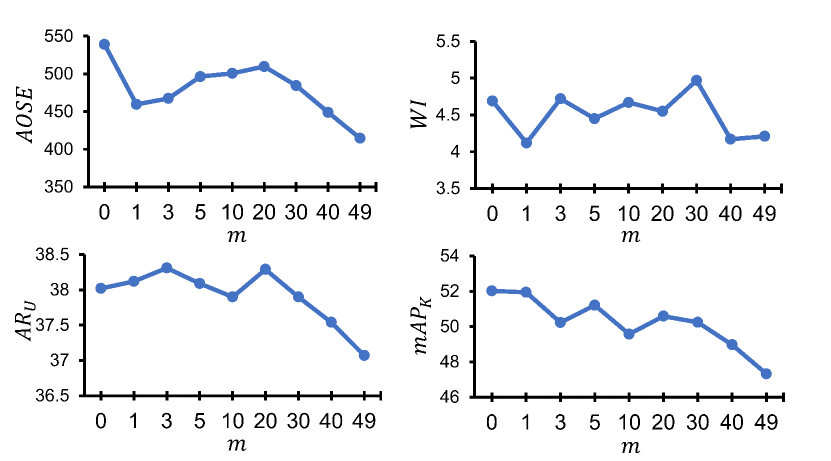
Figure 4: Ablation study of $m$ under the 1-shot VOC10-5-5 experimental setting.

Table 3: Ablation study of proposed components under the 1-shot VOC10-5-5 experimental setting.

$\boldsymbol{L}_{align}^{S}$	$\boldsymbol{L}_{align}^{V}$	$\boldsymbol{L}_{CED}$	$\boldsymbol{L}_{AC}$	$WI$	$AOSE$	$mAP_{K}$	$R_{U}$	$AR_{U}$
✔				7.06	2314.10	57.79	0.00	0.00
✔	✔			6.83	2169.10	58.66	0.00	0.00
✔		✔		5.17	615.80	49.76	79.63	37.96
✔		✔	✔	4.95	567.60	51.93	79.38	37.94
✔	✔	✔		4.69	539.10	52.02	79.93	38.02
✔	✔	✔	✔	4.12	459.60	51.94	79.88	38.12
Conditional energy [40]				4.57	896.00	52.39	78.90	35.54
Evidential uncertainty [41]				4.87	884.00	52.95	78.79	34.35
Gradient-based attribution (Ours)				4.12	459.60	51.94	79.88	38.12

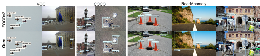
Figure 5: The visualized results on VOC, COCO, and RoadAnomaly [21] datasets under 10-shot VOC10-5-5 setting.

4.3 Ablation Studies

Ablation of pseudo-unknown mining method. We ablate the proposed pseudo-unknown mining method under the 1-shot VOC10-5-5 experimental setting, as shown in Tab. 4 (bottom). Compared to previous state-of-the-art mining approaches, our method achieves the best performance on unknown metrics, with $AR_{U}$, $WI$ and $AOSE$ outperforming the evidential uncertainty [41] by 3.77%, 0.75 and 424.40, and achieves competitive result on $mAP_{K}$. It indicates that gradient-based attribution method, from the perspective of output interpretability, can better filter high-uncertainty pseudo-unknown samples for subsequent decoupled training.

Ablation of proposed loss functions. We ablate the proposed losses under the 1-shot VOC10-5-5 experimental setting, as shown in Tab. 4 (top). The proposed $\boldsymbol{L}_{align}^{V}$ assists in obtaining better semantic class clusters, which improves the accuracy of known classes while enhancing all metrics for unknown rejection. By employing attribution gradients to filter pseudo-unknown samples, the proposed $\boldsymbol{L}_{CED}$ establishes discriminative decision boundaries between known and unknown classes through decoupled evidential learning. The regularization with $\boldsymbol{L}_{AC}$ yields improved $WI$ and $AOSE$ without adversely affecting $mAP_{K}$, indicating its facilitation in the formation of decision boundaries.

Ablation of abnormal gradient feature number $m$. We ablate the abnormal feature number $m$ under the 1-shot VOC10-5-5 experimental setting, as shown in Fig. 4. The results indicate that including non-abnormal values in training compromises the precision of known classes and hinders the formation of effective unknown decision boundaries. Considering the best overall performance and additional computational overhead, we choose $m=1$ by default.

5 Conclusion

In this paper, we introduce a novel approach to address the sophisticated few-shot open-set detection problem. We apply prompt learning to the FOOD task for the first time, supplemented by contrastive learning in the visual space to encourage the formation of semantic clusters. Recognizing that the training data may not adequately cover the distribution of unknown classes, we innovatively mine samples with high uncertainty as pseudo-unknown samples with gradient-based attribution. We employ a conditional evidence decoupling loss and a local anomaly gradient calibration loss to learn information about unknown classes and establish a discriminative decision boundary for unknown rejection. Extensive experiments demonstrate that our proposed method significantly outperforms existing methods and achieves new state-of-the-art results.

supplemental material

Appendix A Analysis of aggregated attribution gradients

We explain the rationale behind designing Eq. 5 to aggregate attribution gradients as a measure of uncertainty. Given the network output $f(\boldsymbol{z})$ of an input vector $\boldsymbol{z}=[z_{1},\cdots,z_{n}]$, it can be represented using a K-th order Taylor expansion [6] as:

$${f(\boldsymbol{z})=f(\boldsymbol{b})+\sum_{i=1}^{n}\frac{1}{1!}\cdot\frac{\partial f(\boldsymbol{b})}{\partial z_{i}}\cdot\left(z_{i}-b_{i}\right)+\sum_{i=1}^{n}\sum_{j=1}^{n}\frac{1}{2!}\cdot\frac{\partial^{2}f(\boldsymbol{b})}{\partial z_{i}\partial z_{j}}\cdot\left(z_{i}-b_{i}\right)\left(z_{j}-b_{j}\right)+\cdots+\epsilon_{K}},$$ (17)

where $\boldsymbol{b}$ is a baseline point and $\epsilon_{K}$ denotes the approximation error. Furthermore, the contribution of each input feature $z_{i}$ to the output can be expressed as the sum of Taylor independent effect $I(\boldsymbol{\kappa})$ and Taylor interaction effect $\phi(\boldsymbol{\kappa})$:

$${a_{i}=w_{i,\boldsymbol{\kappa}}^{\phi}\phi(\boldsymbol{\kappa})+w_{i,\boldsymbol{\kappa}}^{I}I(\boldsymbol{\kappa})},$$ (18)

where $\boldsymbol{\kappa}=\left[\kappa_{i},\cdots,\kappa_{n}\right]\in\mathbb{N}^{n}$ denotes the degree vector of the input variable $z_{i}$, $w_{i,\boldsymbol{\kappa}}^{\phi}$ and $w_{i,\boldsymbol{\kappa}}^{I}$ represents the ratio of a specific Taylor interaction effect and Taylor independent effect, respectively. The interaction effect $\phi(\boldsymbol{\kappa})$ contains at least two $\kappa_{i}>0$ and $\kappa_{j}>0$ in $\boldsymbol{\kappa}$, which indicate the contribution of the interaction of input variables to the output. The independent effect $I(\boldsymbol{\kappa})$ constraints only one $\kappa_{i}>0$ in $\boldsymbol{\kappa}$, which indicates the independent contribution of input variables to the output.

GAIA’s [5] observations indicated OOD samples exhibit a greater prevalence of non-zero attribution gradients compared to ID samples, they have proved that a zero gradient for a particular feature $z_{i}$ implies null independent and interaction effects, denoting negligible contribution to network output ($a_{i}=0$). For ID class samples, network attention is concentrated on specific features for final classification, resulting in a predominance of zero feature gradients. Conversely, network attention may be more dispersed for unfamiliar samples, which yields a higher incidence of non-zero gradients. Thus, we multiply the sum of non-zero gradients for each channel by the sum of the absolute values of the gradients, which could enhance the channel-wise average abnormality mentioned in GAIA [5], thereby obtaining a more robust uncertainty score.

Table 4: The Average Recall ($AR$) of objects on VOC10-5-5/VOC-COCO test datasets with different independent RPN types.

	$S_{obj}$	$\sqrt{S_{obj}\cdot S_{center}}$
VOC10-5-5	56.90	57.40
VOC-COCO	38.10	40.20

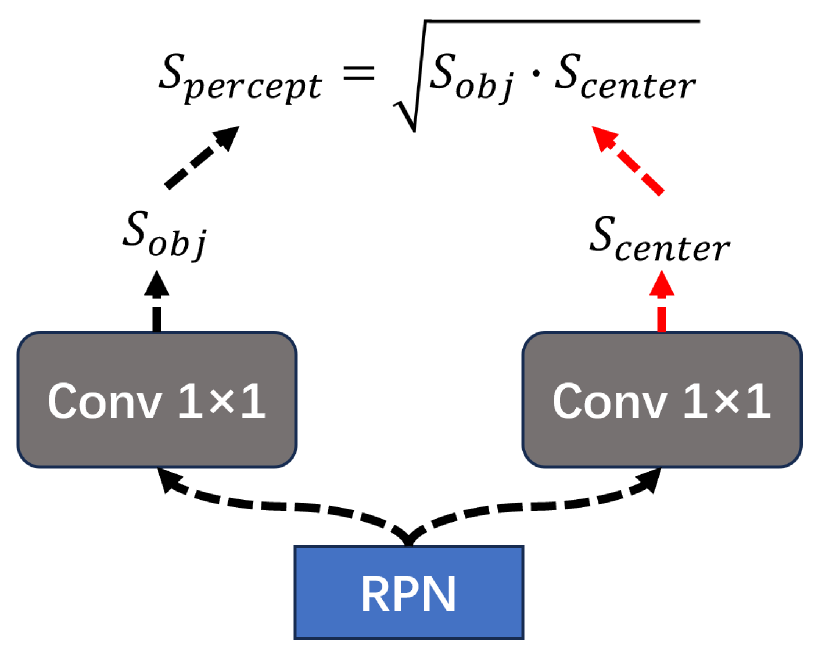
Figure 6: Independently trained RPN structure.

Appendix B Additional experimental results

B.1 Experiments of independently trained RPN

We utilize an independently trained backbone for the RPN and attach a centerness [46] branch parallel to the original objectness branch (in Fig. 6), which can alleviate the issue of overfitting to known classes in the original RPN. For each anchor position $(x,y)$, we can compute the centerness with respect to the ground-truth box $(x_{0},y_{0},x_{1},y_{1})$:

$$\begin{array}[]{r}centerness_{x,y}^{*}=\sqrt{\frac{\min\left(l^{*},r^{*}\right)}{\max\left(l^{*},r^{*}\right)}\times\frac{\min\left(t^{*},b^{*}\right)}{\max\left(t^{*},b^{*}\right)}},\\ \\ \text{ where, }\quad l^{*}=x-x_{0},\quad t^{*}=y-y_{0},\\ r^{*}=x_{1}-x,\quad b^{*}=y_{1}-y.\end{array}$$ (19)

As shown in Tab. 6, we conduct experiments on the choice of final object scores, which are trained only on the objectness branch and both two branches. The results show that for both VOC10-5-5 and VOC-COCO settings, our RPN structure and final object scores can perform better on average recall ($AR$) of objects.

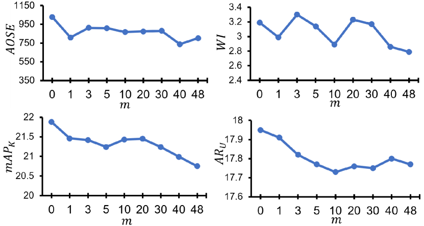
Figure 7: Ablation study of $m$ under the 5-shot VOC-COCO experimental setting.

Table 5: Ablation study of $k$ and $S_{fg:bg}$ under the 1-shot VOC10-5-5 experimental setting.

$k$	$S_{fg:bg}$	$WI$	$AOSE$	$mAP_{K}$	$R_{U}$	$AR_{U}$
3	1:3	4.12	459.60	51.94	79.88	38.12
1	1:3	4.05	420.40	48.93	78.47	37.79
5	1:3	4.58	501.17	50.80	79.18	37.96
10	1:3	4.92	588.00	52.22	80.73	38.22
3	1:1	4.35	486.00	50.42	79.44	38.29
3	1:2	4.01	439.00	50.87	79.33	37.80
3	1:5	4.33	452.20	50.49	80.25	37.99

B.2 Ablation study of $m$ on VOC-COCO datasets

As shown in Fig 7, we also conduct ablation experiments on the selection of the number of abnormal local features $m$ under the 5-shot VOC-COCO experimental setting, and discover a pattern similar to that observed in the VOC10-5-5 setting.

B.3 Ablation study of $k$ and $S_{fg:bg}$

We conduct ablation experiments on the number of pseudo-unknown sample mining $k$ and the foreground-background mining ratio $S_{fg:bg}$, as shown in Tab 7. When the ratio $S_{fg:bg}$ remains constant, smaller values of $k$ result in better $WI$ and $AOSE$ but poorer $mAP_{K}$ and $AR_{U}$. Conversely, larger values of $k$ yield better known class accuracy $mAP_{K}$ and $AR_{U}$ but lower $WI$ and $AOSE$. We chose a balanced value of $k=3$. When the mining number $k$ remains constant, mining too few background proposals negatively affects all metrics. Therefore, we selected $S_{fg:bg}=1:3$.

Table 6: Ablation study of prompt context type under VOC10-5-5 experimental setting.

		$WI$	$AOSE$	$mAP_{K}$	$R_{U}$	$AR_{U}$
1-shot	CSC	4.12	459.60	51.94	79.88	38.12
	UC	5.90	700.00	49.41	35.80	76.40
3-shot	CSC	3.72	451.20	53.09	80.55	39.53
	UC	4.96	636.30	51.31	78.51	38.02
5-shot	CSC	3.78	512.20	54.35	81.37	40.32
	UC	4.65	698.70	53.79	79.41	38.73
10-shot	CSC	3.43	546.30	58.55	79.39	39.79
	UC	3.63	656.00	56.90	76.51	37.78

B.4 Ablation study of prompt context type

We conducted ablation experiments on the types of context used in prompt learning, specifically including Unified Context (UC) and Class-Specific Context (CSC). As shown in Tab. 6, we found that using CSC consistently outperforms UC. This may be because the object detection task generates diverse proposals, and using CSC can better capture the features of different classes.

Appendix C More visualization results

Fig. 8 presents additional visualization results of our approach on the VOC, COCO, and RoadAnomaly datasets. It can be observed that our method demonstrates a capacity to perceive numerous objects present in the images and establish decision boundaries effectively for their classification.

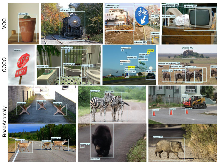
Figure 8: More visualization results on VOC, COCO, and RoadAnomaly [21] datasets under 10-shot VOC10-5-5 setting.

Appendix D Broader impact and limitations

This paper proposes a solution for few-shot open-set object detection, potentially applicable to real-world scenarios such as obstacle detection in autonomous driving. It is possible to achieve good generalization to unknown classes by training with limited annotated data. However, there are still limitations in performing gradient attribution on image encoders based on transformer architectures such as ViT, which will be the focus of our future research.

References

- [1] Sima Behpour, Thang Long Doan, Xin Li, Wenbin He, Liang Gou, and Liu Ren. Gradorth: A simple yet efficient out-of-distribution detection with orthogonal projection of gradients. Advances in Neural Information Processing Systems, 36, 2023.
- [2] Malik Boudiaf, Etienne Bennequin, Myriam Tami, Antoine Toubhans, Pablo Piantanida, Celine Hudelot, and Ismail Ben Ayed. Open-set likelihood maximization for few-shot learning. In Proceedings of the IEEE/CVF Conference on Computer Vision and Pattern Recognition, pages 24007–24016, 2023.
- [3] Nicolas Carion, Francisco Massa, Gabriel Synnaeve, Nicolas Usunier, Alexander Kirillov, and Sergey Zagoruyko. End-to-end object detection with transformers. In European conference on computer vision, pages 213–229. Springer, 2020.
- [4] Aditya Chattopadhay, Anirban Sarkar, Prantik Howlader, and Vineeth N Balasubramanian. Grad-cam++: Generalized gradient-based visual explanations for deep convolutional networks. In 2018 IEEE winter conference on applications of computer vision (WACV), pages 839–847. IEEE, 2018.
- [5] Jinggang Chen, Junjie Li, Xiaoyang Qu, Jianzong Wang, Jiguang Wan, and Jing Xiao. Gaia: Delving into gradient-based attribution abnormality for out-of-distribution detection. Advances in Neural Information Processing Systems, 36, 2023.
- [6] Huiqi Deng, Na Zou, Mengnan Du, Weifu Chen, Guocan Feng, Ziwei Yang, Zheyang Li, and Quanshi Zhang. Understanding and unifying fourteen attribution methods with taylor interactions. arXiv preprint arXiv:2303.01506, 2023.
- [7] Andrija Djurisic, Nebojsa Bozanic, Arjun Ashok, and Rosanne Liu. Extremely simple activation shaping for out-of-distribution detection. International Conference on Learning Representations, 2023.
- [8] Xuefeng Du, Zhaoning Wang, Mu Cai, and Yixuan Li. Vos: Learning what you don’t know by virtual outlier synthesis. International Conference on Learning Representations, 2022.
- [9] Mark Everingham, Luc Van Gool, Christopher KI Williams, John Winn, and Andrew Zisserman. The pascal visual object classes (voc) challenge. International journal of computer vision, 88:303–338, 2010.
- [10] Ross Girshick. Fast r-cnn. In Proceedings of the IEEE international conference on computer vision, pages 1440–1448, 2015.
- [11] Xiaoyuan Guan, Zhouwu Liu, Wei-Shi Zheng, Yuren Zhou, and Ruixuan Wang. Revisit pca-based technique for out-of-distribution detection. In Proceedings of the IEEE/CVF International Conference on Computer Vision, pages 19431–19439, 2023.
- [12] Jiaming Han, Yuqiang Ren, Jian Ding, Xingjia Pan, Ke Yan, and Gui-Song Xia. Expanding low-density latent regions for open-set object detection. In Proceedings of the IEEE/CVF Conference on Computer Vision and Pattern Recognition, pages 9591–9600, 2022.
- [13] Kaiming He, Xiangyu Zhang, Shaoqing Ren, and Jian Sun. Deep residual learning for image recognition. In Proceedings of the IEEE conference on computer vision and pattern recognition, pages 770–778, 2016.
- [14] Minki Jeong, Seokeon Choi, and Changick Kim. Few-shot open-set recognition by transformation consistency. In Proceedings of the IEEE/CVF Conference on Computer Vision and Pattern Recognition, pages 12566–12575, 2021.
- [15] Audun Jøsang. Subjective logic, volume 3. Springer, 2016.
- [16] KJ Joseph, Salman Khan, Fahad Shahbaz Khan, and Vineeth N Balasubramanian. Towards open world object detection. In Proceedings of the IEEE/CVF conference on computer vision and pattern recognition, pages 5830–5840, 2021.
- [17] Dahun Kim, Tsung-Yi Lin, Anelia Angelova, In So Kweon, and Weicheng Kuo. Learning open-world object proposals without learning to classify. IEEE Robotics and Automation Letters, 7(2):5453–5460, 2022.
- [18] Nishant Kumar, Siniša Šegvić, Abouzar Eslami, and Stefan Gumhold. Normalizing flow based feature synthesis for outlier-aware object detection. In Proceedings of the IEEE/CVF Conference on Computer Vision and Pattern Recognition, pages 5156–5165, 2023.
- [19] Tsung-Yi Lin, Priya Goyal, Ross Girshick, Kaiming He, and Piotr Dollár. Focal loss for dense object detection. In Proceedings of the IEEE international conference on computer vision, pages 2980–2988, 2017.
- [20] Tsung-Yi Lin, Michael Maire, Serge Belongie, James Hays, Pietro Perona, Deva Ramanan, Piotr Dollár, and C Lawrence Zitnick. Microsoft coco: Common objects in context. In Computer Vision–ECCV 2014: 13th European Conference, Zurich, Switzerland, September 6-12, 2014, Proceedings, Part V 13, pages 740–755. Springer, 2014.
- [21] Krzysztof Lis, Krishna Nakka, Pascal Fua, and Mathieu Salzmann. Detecting the unexpected via image resynthesis. In Proceedings of the IEEE/CVF International Conference on Computer Vision, pages 2152–2161, 2019.
- [22] Bo Liu, Hao Kang, Haoxiang Li, Gang Hua, and Nuno Vasconcelos. Few-shot open-set recognition using meta-learning. In Proceedings of the IEEE/CVF Conference on Computer Vision and Pattern Recognition, pages 8798–8807, 2020.
- [23] Weitang Liu, Xiaoyun Wang, John Owens, and Yixuan Li. Energy-based out-of-distribution detection. Advances in neural information processing systems, 33:21464–21475, 2020.
- [24] Haodong Lu, Dong Gong, Shuo Wang, Jason Xue, Lina Yao, and Kristen Moore. Learning with mixture of prototypes for out-of-distribution detection. International Conference on Learning Representations, 2024.
- [25] Dimity Miller, Lachlan Nicholson, Feras Dayoub, and Niko Sünderhauf. Dropout sampling for robust object detection in open-set conditions. In 2018 IEEE International Conference on Robotics and Automation (ICRA), pages 3243–3249. IEEE, 2018.
- [26] Yifei Ming, Ziyang Cai, Jiuxiang Gu, Yiyou Sun, Wei Li, and Yixuan Li. Delving into out-of-distribution detection with vision-language representations. Advances in neural information processing systems, 35:35087–35102, 2022.
- [27] Atsuyuki Miyai, Qing Yu, Go Irie, and Kiyoharu Aizawa. Locoop: Few-shot out-of-distribution detection via prompt learning. Advances in Neural Information Processing Systems, 36, 2023.
- [28] Sayak Nag, Dripta S Raychaudhuri, Sujoy Paul, and Amit K Roy-Chowdhury. Reconstruction guided meta-learning for few shot open set recognition. IEEE Transactions on Pattern Analysis and Machine Intelligence, 2023.
- [29] Jun Nie, Yonggang Zhang, Zhen Fang, Tongliang Liu, Bo Han, and Xinmei Tian. Out-of-distribution detection with negative prompts. In International Conference on Learning Representations, 2024.
- [30] Limeng Qiao, Yuxuan Zhao, Zhiyuan Li, Xi Qiu, Jianan Wu, and Chi Zhang. Defrcn: Decoupled faster r-cnn for few-shot object detection. In Proceedings of the IEEE/CVF International Conference on Computer Vision, pages 8681–8690, 2021.
- [31] Alec Radford, Jong Wook Kim, Chris Hallacy, Aditya Ramesh, Gabriel Goh, Sandhini Agarwal, Girish Sastry, Amanda Askell, Pamela Mishkin, Jack Clark, et al. Learning transferable visual models from natural language supervision. In International conference on machine learning, pages 8748–8763. PMLR, 2021.
- [32] Joseph Redmon, Santosh Divvala, Ross Girshick, and Ali Farhadi. You only look once: Unified, real-time object detection. In Proceedings of the IEEE conference on computer vision and pattern recognition, pages 779–788, 2016.
- [33] Shaoqing Ren, Kaiming He, Ross Girshick, and Jian Sun. Faster r-cnn: Towards real-time object detection with region proposal networks. Advances in neural information processing systems, 28, 2015.
- [34] Hiran Sarkar, Vishal Chudasama, Naoyuki Onoe, Pankaj Wasnik, and Vineeth N Balasubramanian. Open-set object detection by aligning known class representations. In Proceedings of the IEEE/CVF Winter Conference on Applications of Computer Vision, pages 219–228, 2024.
- [35] Ramprasaath R Selvaraju, Michael Cogswell, Abhishek Das, Ramakrishna Vedantam, Devi Parikh, and Dhruv Batra. Grad-cam: Visual explanations from deep networks via gradient-based localization. In Proceedings of the IEEE international conference on computer vision, pages 618–626, 2017.
- [36] Murat Sensoy, Lance Kaplan, and Melih Kandemir. Evidential deep learning to quantify classification uncertainty. Advances in neural information processing systems, 31, 2018.
- [37] Kari Sentz and Scott Ferson. Combination of evidence in dempster-shafer theory. Sandia National Lab.(SNL-NM), Albuquerque, NM (United States), 2002.
- [38] Yang Shu, Xingzhuo Guo, Jialong Wu, Ximei Wang, Jianmin Wang, and Mingsheng Long. Clipood: Generalizing clip to out-of-distributions. In International Conference on Machine Learning, pages 31716–31731. PMLR, 2023.
- [39] Karen Simonyan, Andrea Vedaldi, and Andrew Zisserman. Deep inside convolutional networks: Visualising image classification models and saliency maps. arXiv preprint arXiv:1312.6034, 2013.
- [40] Binyi Su, Hua Zhang, Jingzhi Li, and Zhong Zhou. Toward generalized few-shot open-set object detection. IEEE Transactions on Image Processing, 33:1389–1402, 2024.
- [41] Binyi Su, Hua Zhang, and Zhong Zhou. Hsic-based moving weight averaging for few-shot open-set object detection. In Proceedings of the 31st ACM International Conference on Multimedia, pages 5358–5369, 2023.
- [42] Yiyou Sun, Chuan Guo, and Yixuan Li. React: Out-of-distribution detection with rectified activations. Advances in Neural Information Processing Systems, 34:144–157, 2021.
- [43] Yiyou Sun and Yixuan Li. Dice: Leveraging sparsification for out-of-distribution detection. In European Conference on Computer Vision, pages 691–708. Springer, 2022.
- [44] Yiyou Sun and Yixuan Li. Opencon: Open-world contrastive learning. Transactions on Machine Learning Research, 2023.
- [45] Leitian Tao, Xuefeng Du, Xiaojin Zhu, and Yixuan Li. Non-parametric outlier synthesis. International Conference on Learning Representations, 2023.
- [46] Zhi Tian, Chunhua Shen, Hao Chen, and Tong He. Fcos: A simple and strong anchor-free object detector. IEEE Transactions on Pattern Analysis and Machine Intelligence, 44(4):1922–1933, 2020.
- [47] Haoqi Wang, Zhizhong Li, Litong Feng, and Wayne Zhang. Vim: Out-of-distribution with virtual-logit matching. In Proceedings of the IEEE/CVF conference on computer vision and pattern recognition, pages 4921–4930, 2022.
- [48] Haoyu Wang, Guansong Pang, Peng Wang, Lei Zhang, Wei Wei, and Yanning Zhang. Glocal energy-based learning for few-shot open-set recognition. In Proceedings of the IEEE/CVF Conference on Computer Vision and Pattern Recognition, pages 7507–7516, 2023.
- [49] Hualiang Wang, Yi Li, Huifeng Yao, and Xiaomeng Li. Clipn for zero-shot ood detection: Teaching clip to say no. In Proceedings of the IEEE/CVF International Conference on Computer Vision, pages 1802–1812, 2023.
- [50] Xin Wang, Thomas E Huang, Trevor Darrell, Joseph E Gonzalez, and Fisher Yu. Frustratingly simple few-shot object detection. arXiv preprint arXiv:2003.06957, 2020.
- [51] Yanghao Wang, Zhongqi Yue, Xian-Sheng Hua, and Hanwang Zhang. Random boxes are open-world object detectors. In Proceedings of the IEEE/CVF International Conference on Computer Vision, pages 6233–6243, 2023.
- [52] Yuhang Zang, Hanlin Goh, Josh Susskind, and Chen Huang. Overcoming the pitfalls of vision-language model finetuning for ood generalization. International Conference on Learning Representations, 2024.
- [53] Yiwu Zhong, Jianwei Yang, Pengchuan Zhang, Chunyuan Li, Noel Codella, Liunian Harold Li, Luowei Zhou, Xiyang Dai, Lu Yuan, Yin Li, et al. Regionclip: Region-based language-image pretraining. In Proceedings of the IEEE/CVF Conference on Computer Vision and Pattern Recognition, pages 16793–16803, 2022.
- [54] Da-Wei Zhou, Han-Jia Ye, and De-Chuan Zhan. Learning placeholders for open-set recognition. In Proceedings of the IEEE/CVF conference on computer vision and pattern recognition, pages 4401–4410, 2021.
- [55] Kaiyang Zhou, Jingkang Yang, Chen Change Loy, and Ziwei Liu. Conditional prompt learning for vision-language models. In Proceedings of the IEEE/CVF conference on computer vision and pattern recognition, pages 16816–16825, 2022.
- [56] Kaiyang Zhou, Jingkang Yang, Chen Change Loy, and Ziwei Liu. Learning to prompt for vision-language models. International Journal of Computer Vision, 130(9):2337–2348, 2022.
- [57] Zhongxiang Zhou, Yifei Yang, Yue Wang, and Rong Xiong. Open-set object detection using classification-free object proposal and instance-level contrastive learning. IEEE Robotics and Automation Letters, 8(3):1691–1698, 2023.