Correlation of the L-mode density limit with edge collisionality

Abstract

The “density limit” is one of the fundamental bounds on tokamak operating space, and is commonly estimated via the empirical Greenwald scaling. This limit has garnered renewed interest in recent years as it has become clear that ITER and many tokamak pilot plant concepts must operate near or above the widely-used Greenwald limit to achieve their objectives. Evidence has also grown that the Greenwald scaling - in its remarkable simplicity - may not capture the full complexity of the disruptive density limit. In this study, we assemble a multi-machine database to quantify the effectiveness of the Greenwald limit as a predictor of the L-mode density limit and identify alternative stability metrics. We find that a two-parameter dimensionless boundary in the plasma edge, $\nu_{*\rm,edge}^{\rm limit}=3.0\beta_{T,{\rm edge}}^{-0.4}$, achieves significantly higher accuracy (true negative rate of 97.7% at a true positive rate of 95%) than the Greenwald limit (true negative rate 86.1% at a true positive rate of 95%) across a multi-machine dataset including metal- and carbon-wall tokamaks (AUG, C-Mod, DIII-D, and TCV). The collisionality boundary presented here can be applied for density limit avoidance in current devices and in ITER, where it can be measured and responded to in real time.

Keywords: tokamak, density limit, machine learning

1 Introduction

Plasma electron density ($n_{e}$) is a critical lever for fusion performance in tokamaks. High density is crucial for many burning plasma tokamak concepts to maximize fusion triple product $nT\tau_{E}$ [1], enhance bootstrap current drive (via steeper density gradients in the pedestal) [2], and enable divertor detachment [3]. There has long been an interest in developing scaling laws to describe the highest achieveable density in tokamaks [4, 5, 6]. The most widely utilized empirical density limit scaling today is the “Greenwald limit” [7], expressed as

$$\frac{\bar{n}}{n_{G}}=1,$$ (1)

where $\bar{n}$ is the line averaged electron density in units of $10^{20}$ m^-3, $n_{G}\equiv I_{p}/\pi a^{2}$ is the “Greenwald density,” $I_{p}$ is the plasma current in MA, and $a$ is the minor radius in meters. Operating near or above this limit correlates with confinement regime transitions when the plasma is in the “high” confinement mode (H-mode) and disruptions when the plasma is in the “low” confinement mode (L-mode). Nevertheless, to maximize fusion power, burning plasma experiments such as ITER [8] and fusion power plant (FPP) concepts (such as EU-DEMO [9], the compact advanced tokamak [2], and ARC [10]) are designed to operate near or above the Greenwald limit. Of course, by choosing to operate near an instability density limit, future devices run the risk of harmful transients, such as H-to-L back-transitions and disruptions. Even infrequent unmitigated disruptions - such as once a month - could render tokamak power plants uneconomical given the long timescales needed for repairs [11]. Arguably, tokamak power plants require large safety margins and/or extremely effective control solutions for the density limit and other instabilities.

While a complete first-principles treatment of the density limit remains elusive, theory and experiment have clarified the characteristic dynamics, summarized in Fig. 1. The path to the density limit begins with edge density increasing and/or edge temperature decreasing [12]. Past a certain threshold, a thermal instability occurs at the plasma edge, causing a collapse of the edge temperature. If the plasma was operating in H-mode, it experiences an H-to-L back-transition, referred to as an “H-mode density limit” (HDL). The plasma may stabilize after the HDL, but if edge density continues to rise and/or edge temperature continues to fall, another temperature instability can occur. In L-mode, this edge temperature collapse causes the plasma current channel to shrink from the cold, resistive edge, and concentrate in a peaked current profile [13, 14]. When current channel is sufficiently narrow, it loses MHD stability, causing a disruption described as an “L-mode density limit.” The approach to the density limit is commonly associated with the formation and movement of an X-point radiator or a MARFE - a toroidally symmetric ring of cool, dense plasma on the high-field side [15].

Theories attempting to explain the thermal instability tend to come in two flavors: a radiative instability in the edge [16, 17] or enhanced turbulent transport in the edge [18, 19, 20, 21]. It has been shown that many of these models share qualitative similarities to each other [22].

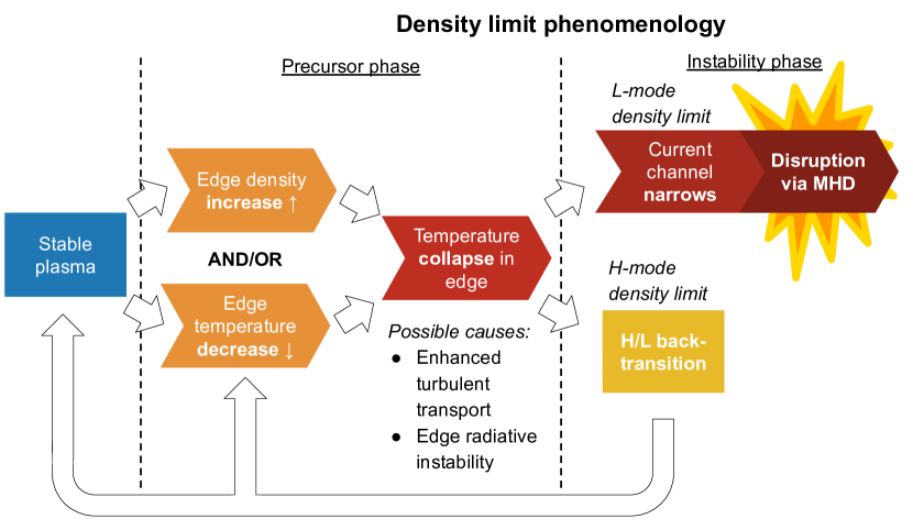
Figure 1: The chain of events characteristic of density limits in tokamaks. If the discharge is in H-mode, it suffers an H-to-L back-transition; this is referred to as an “H-mode density limit.” If it is in L-mode, the plasma eventually disrupts.

This sharpening picture of the density limit suggests that burning plasmas may be able to safely achieve densities above the Greenwald limit. Firstly, the density limit depends on the edge of the plasma, not the core. Experiments have frequently demonstrated $\bar{n}/n_{G}>1$ through peaked density profiles that maintain $n_{\rm edge}/n_{G}<1$ [23, 24, 25, 26, 27]. Experimental observations lead us to believe that we should see density peaking in lower collisionality plasmas [28], thereby potentially enabling $\bar{n}/n_{G}>1$ in burning plasmas.

The second observation is an apparent power scaling of the density limit. Although a power scaling was not clear in earlier experiments [7], evidence from experiments with significant auxiliary heating suggest a modest input power scaling $P^{0.2-0.5}$ augmenting the Greenwald limit [23, 19, 22, 29, 24, 25, 30, 31, 32]. This power dependence is understood to be due to higher input power raising the temperature at the edge and holding off the onset of the temperature instability.

At the same time, we will show in this paper that these two observations alone are not able to achieve the extremely high density limit disruption prediction accuracy needed for ITER system protection [33]. The Greenwald limit was not derived with disruption prediction in mind, and so it is perhaps not surprising that there is room for improvement for a density limit disruption forecaster. It is notable however, that we must go beyond applying a power scaling and using the edge density, and instead utilize the edge temperature and density to predict the density limit stability boundary with the high accuracy .

In this paper, we assemble and study a multi-machine database of L-mode density limit events from Asdex UpGrade (AUG), Alcator C-Mod, DIII-D, EAST, and TCV. We apply a variety of advanced statistical techniques to predict the onset of the triggering instability, thus finding that:

• The Greenwald limit does not universally predict the onset of L-mode density limit events (true negative rate of $<87$% for a true positive rate of 95%).

• A simple dimensionless stability boundary in terms of the effective collisionality and $\beta_{T}$ in the plasma edge, $\nu_{*\rm,edge}^{\rm limit}=3.0\beta_{T,\rm edge}^{-0.41}$, is a reliable proximity-to-density-limit metric in this database (true negative rate of 97.7% for a true positive rate of 95%).

The paper is organized as follows: Section 2 describes the methods used for the dataset assembly and the data-driven analysis, Section 3 describes the prediction performance of various models on an unseen test set, Section 4 discusses the relation to existing density limit observations and considers example discharges from the database, and Section 5 summarizes the findings of this study and outlines future work.

2 Methods

2.1 Dataset and labeling

The dataset utilized for this study is composed of discharges from five tokamaks: AUG, C-Mod, DIII-D, EAST, and TCV. The number of discharges and samples from each device is shown in Table 1, and the engineering parameters of these devices can be found in A, Table 7. The reader should note the significant variations in the number discharges available for each device due to different frequency of density limit experiments, lifetime of the machines, and data availability.

Table 1: Number of unique discharges and time steps in the database assembled for this study, divided into discharges that feature an L-mode density limit (LDL) and those that do not (stable).

• Device	LDL discharges	LDL time steps	Stable discharges	Stable time steps
  AUG	33	1,106	52	18,425
  C-Mod	92	3,819	2,556	279,756
  DIII-D	42	2,225	1,140	375,219
  EAST	13	1,498	708	701,543
  TCV	34	1,563	116	11,539
  Total	214	10,211	4,572	1,386,482

Density limit (DL) discharges were manually labeled by the authors using the pattern observed across all devices: an increase in density/fueling corresponding with a decrease in the edge temperature, followed by the formation of a radiator or MARFE near the X-point, which eventually destabilizes and moves towards the core, resulting in an MHD-driven disruption. For this study L-mode DL (LDL) precursor phase start and end time was manually labeled after the formation of the X-point radiator and before the radiation front moves inward immediately before the disruption. An example of this labeling is schematically represented in Figure 2.

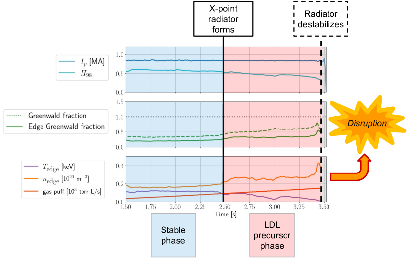
Figure 2: Labeling the L-mode density limit for an example discharge, DIII-D #191793. The LDL precursor phase is the time period between when the X-point radiator forms and when the radiator becomes unstable and moves toward the plasma core. We ignore the short window in time after the radiator is destabilized and the disruption is inevitable. Here, “edge” density and temperature are defined as the average measurement of the quantity between $\rho=$ 0.85 and 0.95.

The C-Mod and DIII-D database of LDLs are newly collated for this study based on workflows utilized in Ref. [34, 35]. The LDL shots from AUG and TCV in this study appeared in Ref. [19], and those from EAST appeared in Ref. [36].

To isolate density limit dynamics from other instabilities, LDL candidates were excluded from the database if the operators noted major impurity injections, the discharge exhibited significant MHD activity prior to the formation of the X-point radiator, or the disruption was immediately proceeded by a sudden shutoff or failure of input power.

Non-disruptive discharges, also referred to here as “stable” discharges, are uniformly sampled from the set of discharges in each device that did not result in a disruption during flattop and did not experience control errors. Stable discharges that experienced minor disruptions were also excluded. A correlation matrix for the full dataset is reported in A.

2.2 Feature set

Table 2 lists the features used in this analysis. Edge density and temperature in this study are defined as the Thomson Scattering measurements averaged between a normalized radius ($\rho$) of 0.85 and 0.95, as was used for experimental validation of an edge density limit in Ref. [19]. A simple fitting procedure was used to determine the profiles of AUG and TCV, while linear interpolation was used for C-Mod and DIII-D. Averaging over this relatively large edge region reduces the impact of measurement noise. Normalized radius is defined in terms of the square root of the normalized toroidal flux for DIII-D data and the square root of the normalized poloidal flux for AUG, TCV, and C-Mod data. All signals are resampled onto a 10ms timebase for consistency.

Table 2: Features in dataset used for this analysis, as well as “features sets” used in analysis: “Engineering” features, “Edge” features, and dimensionless features.

• Symbol	Definition	“Engineering” features	“Edge” features	Dimensionless features
  $\bar{n}$	e- density, line avg.	X
  $P_{\rm in}$	Input power	X
  $n_{\rm edge}$	e- density, edge		X
  $T_{\rm edge}$	e- temperature, edge		X
  $I_{p}$	Plasma current	X	X
  $a$	Minor radius	X
  $R_{0}$	Major radius		X
  $q_{95}$	Safety factor	X	X	X
  $\nu_{*\rm,edge}$	Collisionality, edge			X
  $\beta_{T,\rm edge}$	Toroidal $\beta$, edge			X
  $\rho^{*}_{\rm edge}$	Norm. gyroradius, edge			X

As shown in Table 2, we conduct our analyses using three distinct sets of features: “engineering” features, “edge” features, and dimensionless features. The engineering features are macroscopic plasma parameters that are relatively easy to measure (ex. $\bar{n}$, $I_{p}$). The edge features are similar, but with the line-averaged density and input power replaced with the edge density and temperature, respectively. These latter two parameters are expected to be more predictive of the density limit because they are local to the edge region where the density limit is thought to be triggered. Because of noise in the measurement of edge density and temperature, a Butterworth filter is applied to these signals with a critical frequency of 8 Hz and 6 Hz, respectively. For the sake of cross-device consistency, the same filter is applied to all devices.

We note that while we have measurements for the major radius $R_{0}$, minor radius $a$, and the toroidal magnetic field $B_{T}$, our primary results will only include one of each parameter at a time because of the strongly correlated with each other. We seek to avoid multicollinearity in training models because it can mask true variable interactions. Additionally, we have measurements for inverse aspect ratio $\epsilon$, elongation $\kappa$, and triangularity $\delta$ across our database, but we exclude them from the analysis engine as there is too little variation among these parameters to be of reliable use in the identified scalings

We also analyze a set of dimensionless variables generally following the definitions used in [37], but with ion density and temperature replaced with the electron value. The dimensionless variables we use include $q_{95}$ and the following:

$$\nu_{\rm*,edge}\equiv\frac{\nu_{ii}q_{\rm cyl}R_{0}}{v_{ti}\epsilon^{3/2}}\approx\frac{e^{4}\ln(\Lambda)}{2\pi\epsilon_{0}^{2}}\frac{n_{\rm edge}}{T_{\rm edge}^{2}}\frac{q_{\rm cyl}R_{0}}{\epsilon^{3/2}},$$ (2)

$$\rho_{*,\rm edge}\equiv\frac{\rho_{i}}{a}\approx\frac{\sqrt{m_{i}T_{\rm edge}},}{eB_{T}a},$$ (3)

$$\beta_{T,\rm edge}\equiv\frac{2n_{\rm edge}T_{\rm edge}}{B_{T}^{2}/(2\mu_{0})},$$ (4)

where $\nu_{ii}$ is the ion-ion collision frequency, $q_{\rm cyl}\equiv\frac{2\pi}{\mu_{0}}\frac{B_{T}a^{2}}{I_{p}R_{0}}(\frac{1+\kappa^{2}}{2})$ is the cylindrical safety factor, $v_{ti}$ is the ion thermal speed, $e$ is the elementary charge, $\ln(\Lambda)$ is the Coulomb logarithm, $\epsilon_{0}$ is the permittivity of free space, $\rho_{i}$ is the ion gryoradius, and $m_{i}$ is the ion mass (assumed to be deuterium), and $\mu_{0}$ is the permeability of free space. We use $q_{95}$ instead of $q_{\rm cyl}$ as the fourth feature in the dimensionless feature case to capture effects of shaping (ex. triangularity) not included in the cylindrical approximation.

2.3 Problem formulation and performance metrics

We formulate DL prediction as a supervised classification problem: we will attempt to find a model that will accurately classify plasma states as stable or in the LDL-precursor phase with sufficient warning time before the instability occurs. Following community standards, we will hold out 20% of the discharges as the test set: these discharges will be only used to evaluate the performance of the model. The remainder of the data will be used in the training set for the models to learn on.

A discharge is classified as being in the LDL precursor phase - the “positive” class - for a given alarm threshold if two conditions are met: 1) the instability score rises above the alarm threshold for two or more consecutive time steps (i.e. 10ms assertion time) and 2) the alarm occurs $>30$ ms before the radiator destabilizes. The first condition is intended to prevent spurious alarm triggers due to an anomalous measurement at a single time step, and the second condition discounts predictions that are “too late” for a disruption mitigation system (DMS) to intervene. One could instead define a tardy alarm in terms of the time needed for disruption avoidance, but this would vary depending on tokamak, actuator type, and plasma scenario. For the sake of simplicity, we choose a well-defined DMS timescale for setting the late alarm threshold, and leave a more thorough treatment of disruption avoidance timescales for a later study. Specifically, we choose a minimum warning time of $30$ ms to match the time needed for actuating the ITER DMS [38]. This is a conservative choice, as the density and temperature dynamics on the devices in the database are relatively shorter due to the smaller device sizes and shorter confinement times. We also note that an alarm that occurs significantly before the LDL time is still considered a true positive, as we do not want to penalize a model for providing a long warning time that could be used in practice for LDL avoidance.

We report two performance metrics to capture the trade-off between true positive rate (TPR) and true negative rate (TNR) that occur when we change the alarm sensitivity: area under the curve (AUC) and the TNR at a fixed TPR of 95% (shorthand: TNR @ TPR = 95%). The AUC is the average TPR across the range of TNR $\in[0,1]$, giving a measurement of the performance across the full range of alarm sensitivities. The TNR @ TPR = 95%, by contrast, represents the proportion of stable discharges that are correctly classified when we require exceptional detection performance of LDLs. The latter is important for ITER and future tokamak power plants, where the potential damage from disruptions necessitates near-perfect (TPR $\geq 95$%) prediction of disruptions.

2.4 DL prediction models

We evaluate four total sequence-to-sequence architectures that fall into two categories: non-symbolic and symbolic. The two non-symbolic models are standard ML workhorses - the neural network (NN) and random forest (RF). Details about hyperparameters scans are reported in B. Hyperparameters are selected via the maximum AUC on the validation set, a randomly assigned set of 20% of discharges withheld from training set.

We also attempt to find a symbolic density limit boundary using two methods: linear regression (LR) and linear support vector machines (LSVM). Symbolic models are simply models that take on an analytic form (for example, the Greenwald fraction is a symbolic model). To identify the linear regression boundary, we average over the last 50 ms before the LDL and use multivariate linear regression to find a power law that minimizes the mean squared error over the training set. We encourage a parsimonious model by computing the p-value of each feature, removing the feature with the largest p-value above 0.05, and re-training until all features in the regression model have p-values less than 0.05. We find a power law boundary using LSVMs by training a classifier on all data points (as with the NN and RF). Feature combinations are explored using sequential feature selection with backward elimination using the Bayesian Information Criterion as the evaluation metric,

$${\rm BIC}=-2\ln(L)+k\ln(s),$$ (5)

where $L$ is the likelihood of the model evaluated on the training set, $k$ is the number of regression variables in the model, and $s$ is the number of samples. BIC balances a reward for low error (low negative log-likelihood) with a penalty for more parameters in the model, weighted by the log of the number of samples used to fit the parameters. As plasmas states are dynamically evolving in time during discharges and not independently sampled, we approximate $s$ as the number of discharges. We similarly adjust the likelihood $\sum y\ln(p)+(1-y)\log(1-p)$ by rescaling it by the ratio of number of discharges to number of time steps.

Finally, we will compare the model predictions with that of the Greenwald fraction using the line-average density and the edge density. These scalings will be used as baselines for comparison to the data-driven approaches.

3 Results

3.1 Predicting the LDL with “engineering” features

Table 3 shows the test set performance of L-mode density limit (LDL) prediction trained on the “engineering” features (Table 2) in comparison to the Greenwald density limit scaling. The symbolic boundaries are all written as proportionalities because different coefficients correspond to different alarm thresholds.

Table 3: The test set performance of LDL prediction for models trained on the engineering features, as well as the Greenwald fraction.

• Model	Analytic boundary	AUC	TNR @ TPR = 95%
  NN	N/A	0.970	81.6%
  RF	N/A	0.942	84.8%
  LSVM	$\bar{n}^{\rm limit}\sim\frac{I_{p}^{0.82}}{a^{1.85}}P_{\rm in}^{0.25}q_{95}^{0.33}$	0.940	75.8%
  Lin. Reg.	$\bar{n}^{\rm limit}\sim\frac{I_{p}^{0.83}}{a^{2.00}}P_{\rm in}^{0.12}q_{95}^{0.47}$	0.927	53.5%
  Greenwald	$\bar{n}^{\rm limit}\sim\frac{I_{p}}{\pi a^{2}}$	0.894	53.9%

We find that the NN, RF, and LSVM have among the best performance, far exceeding the AUC and TNR @ TPR = 95% of the Greenwald scaling. The linear regression model, by contrast has performance more akin to the Greenwald scaling. Interestingly, the LSVM takes the form a Greenwald-like scaling with lower current dependence and additional - but modest - $P_{\rm in}$ and $q_{95}$ dependencies. We plot the density and the product of the remaining variables for the LSVM power law in Fig. 3.

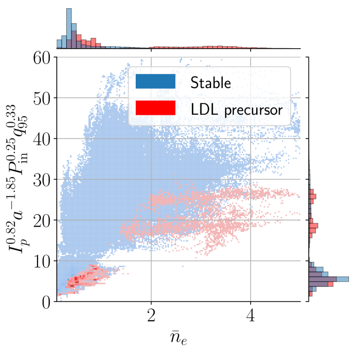
(a) Labeled time steps

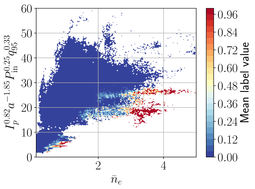
(b) Mean label value

Figure 3: The distribution of line averaged density vs. the remaining terms of the LSVM power law (Table 3) across the database. Subplot 3(a) shows the LDL points (red) superimposed on the non-DL points (green), while 3(b) shows a “stability” heat map, where labels (“stable” = 0, LDL precursor = 1) have been averaged in each bin.

Although the non-symbolic models (NN and RF) achieve the highest performance of all, we note that a TNR of $~{}80$% would be very costly for ITER and FPPs, it would imply around 20% of discharges would be mitigated unnecessarily.

3.2 Predicting the LDL with “edge” features

Because not all discharges in our dataset have edge density measurements, the dataset for the “edge” feature analysis has a different composition of discharges, shown in Table 4. Particularly of note is the absence of EAST data, due to limited diagnostic availability for edge density or temperature measurements. The change in composition of the training and test set results in slightly different performance for the Greenwald scalings compared to the previous section.

Table 4: Number of unique discharges and time steps in the database that have edge density and temperature measurements. These data are used for the analysis in section 3.2 and 3.3.

• Device	LDL discharges	LDL time steps	Stable discharges	Stable time steps
  AUG	30	1,063	49	17,717
  C-Mod	52	3,322	2,210	243,221
  DIII-D	41	2,205	1,043	343,323
  EAST	0	0	0	0
  TCV	30	1,384	67	6,405
  Total	153	7,974	3,369	610,666

As shown in Table 5, the LSVM power law achieves nearly as good performance as the NN and RF, with similar AUC and TNR @ TPR = 95%. The LSVM boundary takes the form of

$$n_{\rm edge}^{\rm limit}\sim\frac{I_{p}^{0.65}}{R_{0}^{1.43}}T_{\rm edge}^{0.99}.$$ (6)

This scaling suggests that devices with higher edge temperatures, higher current, and smaller size can achieve higher absolute densities without disrupting. We show the state space of the edge density vs. the remaining product of the LSVM power law in Fig. 4. We see good separation of the stable and LDL precursor phases, reflecting the high accuracy of this power law in discriminating the LDL precursor phase.

Table 5: The test set performance of LDL prediction for models trained on the edge features, as well as the Greenwald fraction and Edge Greenwald fraction.

• Model	Analytic boundary	AUC	TNR @ TPR = 95%
  NN	N/A	0.998	98.4%
  RF	N/A	0.997	99.1%
  LSVM	$n_{\rm edge}^{\rm limit}\sim\frac{I_{p}^{0.65}}{R_{0}^{1.43}}T_{\rm edge}^{0.99}$	0.997	98.4%
  Lin. Reg.	$n_{\rm edge}^{\rm limit}\sim\frac{I_{p}^{0.63}}{R_{0}^{1.52}}T_{\rm edge}^{0.14}q_{95}^{0.47}$	0.887	46.2%
  Greenwald	$\bar{n}^{\rm limit}\sim\frac{I_{p}}{\pi a^{2}}$	0.971	86.1%
  Edge Greenwald	$n_{\rm edge}^{\rm limit}\sim\frac{I_{p}}{\pi a^{2}}$	0.888	56.7%

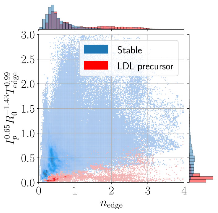
(a) Labeled time steps

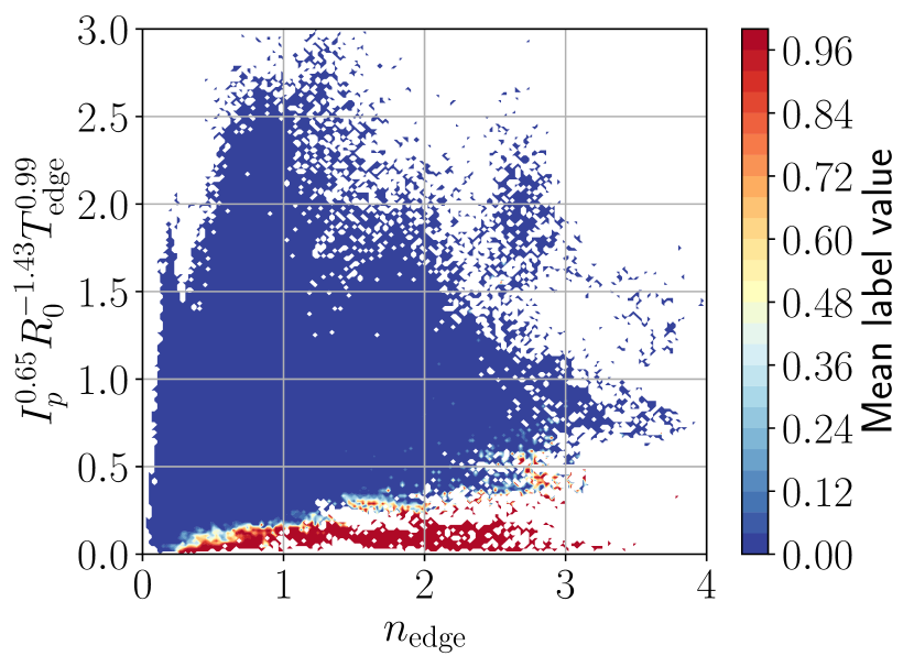
(b) Mean label value

Figure 4: The distribution of edge density vs. the remaining terms of the LSVM power law for the database (Table 5). Subplot 4(a) shows the LDL points (red) superimposed on the non-DL points (green), while 4(b) shows a “stability” heat map, where labels (“stable” = 0, LDL precursor = 1) have been averaged in each bin.

The NN, RF, and LSVM achieve vastly higher performance compared to the engineering feature case (section 3.1) due to the presence of density and edge temperature signals together. Removing either significantly reduces the prediction performance.

Notably, the linear regression power law performs significantly worse compared to the LSVM power law. The form of the boundaries are similar except for a much lower edge temperature exponent for the linear regression and the addition of a moderate $q_{95}$ dependence. The lack of a strong temperature dependence is primarily responsible for the much diminished performance, as this is a key parameter in distinguishing the LDL precursor phase from the stable cases. We can only achieve reliable LDL prediction using a classification heuristic (LSVM) to identify a power law for the LDL boundary; applying linear regression to the density before the onset of the instability leads to significantly lower LDL prediction success.

The theoretical scalings also have higher performance compared to the results section 3.1, due to the differences in the test dataset, as stated earlier, but they still achieve performances far lower than the LSVM, NN, and RF.

3.3 Dimensionless scalings

When trained on the dimensionless set of features $\nu_{*,\rm edge}$, $\rho_{*,\rm edge}$, $\beta_{T,\rm edge}$, and $q_{95}$, the data-driven models achieve similarly excellent performance as is found in the edge features case (section 3.2). The test set performance metrics are reported in Table 6.

Table 6: The test set performance of LDL prediction for models trained on the dimensionless features, as well as the Greenwald fraction and Edge Greenwald fraction.

• Model	Analytic boundary	AUC	TNR @ TPR = 95%
  NN	N/A	0.994	97.3%
  RF	N/A	0.995	97.0%
  LSVM	$\nu_{*\rm,edge}^{\rm limit}\sim\beta_{T,\rm edge}^{-0.41}$	0.996	97.7%
  Lin. Reg.	$\nu_{*\rm,edge}^{\rm limit}\sim\beta_{T,\rm edge}^{-0.67}\rho_{*,\rm edge}^{-0.77}$	0.984	93.4%
  Greenwald	$\bar{n}^{\rm limit}\sim\frac{I_{p}}{\pi a^{2}}$	0.971	86.1%
  Edge Greenwald	$n_{\rm edge}^{\rm limit}\sim\frac{I_{p}}{\pi a^{2}}$	0.888	56.7%

The NN, RF, and LSVM all achieve similar performance as in the previous section (subsection 3.2). There is a very small performance penalty for using dimensionless variables to predict the LDL in this dataset. One difference in this case is that the LSVM has a slightly higher AUC and TNR @ TPR = 95% than the RF and NN. The power law boundary identified by the LSVM is

$$\nu_{*\rm,edge}^{\rm limit}=3.0\beta_{T,\rm edge}^{-0.41}.$$ (7)

The effective collisionality is the strongest term, with a smaller $\beta_{T,\rm edge}$ dependence. The space defined by these two variables is shown in Fig. 5. Once again, we see strong separation between the stable and LDL precursor points. The strongest individual variable is $\nu_{*,\rm edge}$, which can be seen by the already strong separation in the top marginal plot of Fig. 5(a). The $\beta_{T,\rm edge}^{0.4}$ is indeed secondary, but it improves the accuracy slightly because of the tilt of both the stable and LDL precursor clusters in this plot. It is notable that edge collisionality alone is a less accurate descriptor of the density limit in this database compared to the combination of collisionality and $\beta_{T,\rm edge}$.

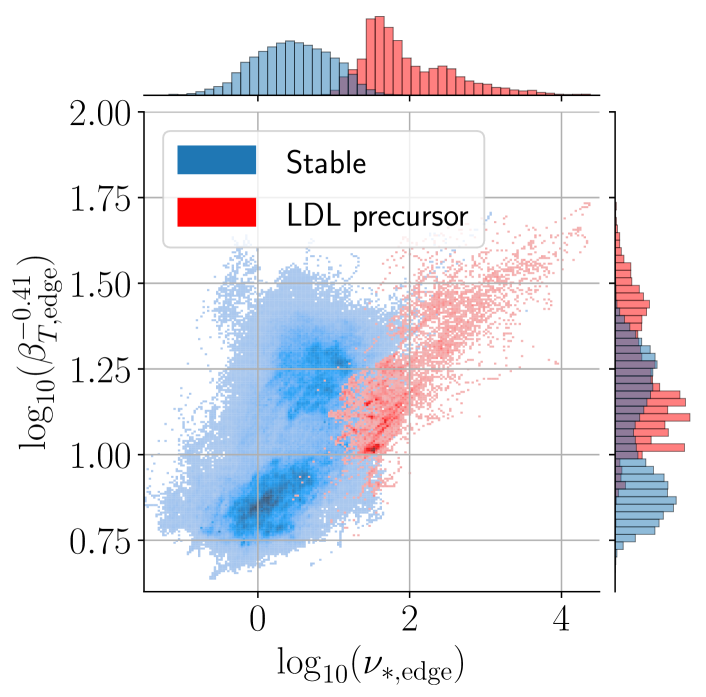
(a) Labeled time steps

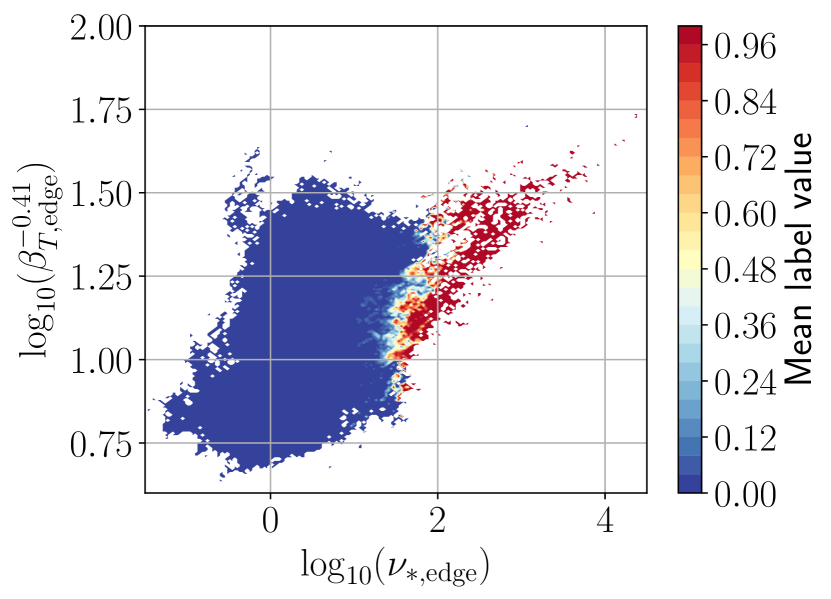
(b) Mean label value

Figure 5: The distribution of edge collisionality versus the other quantity identified by the LSVM power law, $\beta_{T,\rm edge}^{-0.4}$ (Table 6). Subplot 5(a) shows the LDL points (red) superimposed on the non-DL points (green), while 5(b) shows a “stability” heat map, where labels (“stable” = 0, LDL precursor = 1) have been averaged in each bin.

The similar performances for the LSVM when trained on the edge (subsection 3.2) and dimensionless feature sets suggests that the same pattern is being identified. Indeed, the power law identified in the dimensionless case (eq 7) can be written in a remarkably similar form to that of the edge feature case:

$$\nu_{*,\rm edge}\beta_{T,\rm edge}^{0.4}\sim\frac{n_{\rm edge}^{1.4}}{T_{\rm edge}^{1.6}}\frac{R_{0}^{2}B_{T}^{0.2}\epsilon^{1/2}\kappa}{I_{p}}=\bigg{(}\frac{n_{\rm edge}}{T_{\rm edge}^{1.1}}\frac{R_{0}^{1.4}}{I_{p}^{0.7}}(B_{T}^{0.1}\epsilon^{0.4}\kappa^{0.7})\bigg{)}^{1.4},$$ (8)

where one can see that the parameters in the fractions are nearly identical to the power law identified by the edge parameters (Table 5). The term within the parentheses, $B_{T}^{0.1}\epsilon^{0.4}\kappa^{0.7}$, overall varies weakly across the entire database (mean = 1.2, standard deviation = 0.1). It is interesting that there is a nearly 1-to-1 correspondence between the boundaries identified from different feature sets. Despite the edge features case having more degrees of freedom, it arrives at a nearly identical LDL stability boundary.

4 Discussion

4.1 Relation of results to Greenwald limit

When predicting the density limit with only engineering features (section 3.1), the LSVM model identifies a Greenwald-like scaling for the density limit with additional modest power and $q_{95}$ dependencies. The power scaling of $P_{in}^{0.25}$ is consistent with L-mode density limit studies with significant auxiliary heating published after the original Greenwald scaling paper [7], which report power scalings between $P^{0.15}$ and $P^{0.56}$ [17, 29, 25, 30]. The explicit $I_{P}^{0.83}$ dependence and the implicit $I_{p}^{0.83}q_{95}^{0.33}\sim I_{p}^{0.50}$ dependence is also within the range of density limit current scalings reported between $I_{p}^{0.5}$ and $I_{p}^{1.0}$ [17, 29, 25]. We note that in the case of an ohmic plasma with constant loop voltage (where $P_{\rm in}\sim I_{p}$), the database-derived scalings presented here would both go as $\bar{n}^{\rm limit}\sim I_{p}^{\approx 1}$, agreeing with the Greenwald scaling.

The accuracy of Greenwald-like scalings, however, is not sufficient for the needs of ITER and FPPs, where we require extremely robust LDL prediction accuracy. This is achieved only by leveraging the edge density and temperature together, as seen in the edge features (subsection 3.2) and dimensionless scalings case (subsection 3.3). Figure 6 shows a plot of the timeslices associated with stable plasmas and the LDL precursor phase for the Greenwald limit and collisionality stability metric (excluding EAST, as there are no edge density or temperature measurements). We see the collisionality metric is able to better discriminate between the LDL precursor phase and stable plasma states.

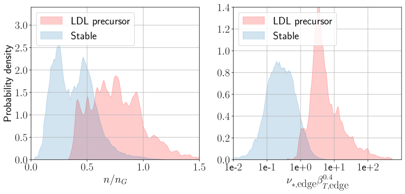
Figure 6: A comparison of the time slices in the stable and LDL precursor phase in terms of both the Greenwald fraction and collisionality boundary metric. The collisionality boundary more clearly separates the precursor phase from stable plasma states.

Notably, the $n^{\rm limit}\sim P_{\rm in}^{0.25}$ and $n^{\rm limit}\sim T_{\rm edge}^{0.99}$ dependencies identified in this study echo the approximation

$$\bar{T}_{e,{\rm sep}}\sim P_{\rm SOL}^{2/7},$$ (9)

where $\bar{T}_{e,{\rm sep}}$ is the average electron temperature at the last closed flux surface and $P_{\rm SOL}\equiv P_{\rm in}-P_{\rm rad}$ is the power through the SOL (input power minus power radiated within the LCFS), which is valid when parallel heat conduction dominates parallel heat convection [39]. Of course $T_{\rm edge}$ is not $\bar{T}_{e}$, and $P_{\rm in}$ is not $P_{\rm SOL}$, but one might expect strong correlations between these parameters in the database.

In summary, the edge and dimensionless scalings are generally consistent with the Greenwald scaling and a moderate power dependence. Nevertheless, extremely robust LDL prediction is only accurately achieved by explicitly accounting for the edge temperature and edge density; a Greenwald scaling with a power dependence does not tell the full story.

4.2 Relation of collisionality boundary to electron adiabaticity

Theoretical treatments of the density limit [18, 40] and empirical studies on individual devices [41, 42] have suggested electron adiabaticity

$$\alpha\equiv\frac{k_{||}^{2}v_{te}^{2}}{\nu_{ee}\omega},$$ (10)

in the plasma edge is a critical parameter for the density limit, where $k_{||}$ is the wavenumber along the magnetic field line (usually taken to be the connection length $L_{c}\sim 1/qR$), $v_{te}$ is the electron thermal speed, $\nu_{ee}$ is the electron-electron collision frequency, and $\omega$ is the peak wave frequency. The regime where $\alpha<1$ is thought to result in edge cooling via increased turbulent transport, caused either through the emergence of Resistive Ballooning Modes (RBMs) [18] or by shear layer collapse [40].

The adiabaticity parameter $\alpha$ is challenging to measure in practice because it involves the peak fluctuation frequency at the plasma edge. We can show, however, that the collisionality boundary (eq. 7) can be re-written in a form similar to the electron adiabaticity. Taking $k_{||}\sim 1/q_{95}R_{0}$ in the plasma edge, similar to [41], one can show

$$(\nu_{*,{\rm edge}}\beta_{T,{\rm edge}}^{0.4})^{-1}\sim\frac{k_{||}^{2}v_{te}^{2}}{\nu_{ee}\omega_{\rm imp}},$$ (11)

where the implied frequency, $\omega_{\rm imp}$, is

$$\omega_{\rm imp}\equiv\frac{T_{\rm edge}^{0.9}}{B_{T}^{0.8}}\frac{n_{\rm edge}^{0.4}k_{||}}{\epsilon^{3/2}}.$$ (12)

The implied frequency has temperature and magnetic field dependencies similar to those of the electron diamagnetic drift frequency

$$\omega_{*e}=\frac{T}{B}\frac{k_{\perp}}{en}\frac{dn}{dr}.$$ (13)

Beyond the leading $T$ and $B$ terms, and the $\epsilon^{3/2}$ term that is relatively fixed across the database, the remaining terms do not obviously agree. We might expect a discrepancy because, as adiabiticity breaks down, we would expect the turbulence to no longer be purely drift waves. Direct measurements of the fluctuation frequency or the density gradient at the edge would help elucidate this matter.

In any case, the similarity of edge collisionality boundary with electron adiabaticity via diamagnetic drift oscillations is notable. It is possible the success of the edge collisionality density limit boundary can be attributed to 1) $\alpha$ causing or correlating with the onset of the density limit and 2) $\omega_{\rm imp}$ serving as a reasonable approximation of the diamagnetic drift frequency for plasma states near the density limit in our database.

4.3 Relation of collisionality boundary to Stroth et al. X-point radiator model [16]

Reference [16] presents a scaling for the formation of X-point radiators (XPRs) by identifying the threshold at which power conducted through the edge of the plasma no longer balances the ionization and charge exchange losses. They estimate the threshold density for XPR formation is

(14)

where $n_{u}^{\rm XPR}$ is the threshold upstream electron ion density for XPR formation, $T_{u}^{5/2}$ is the upstream temperature, $n_{0}$ is the neutral density, $f_{\rm exp}$ is the flux expansion factor, and $q_{s}$ is the safety factor of a cylindrical plasma. If we take the neutral density to be proportional to the upstream density (as suggested in Ref. [22]), take the upstream density and temperature to correspond to the edge density and temperature, and assume roughly fixed flux expansion in the XPR region across these devices, we arrive at a stability limit that goes as

$$n_{\rm edge}^{\rm limit}\sim\frac{T_{\rm edge}^{5/4}\sqrt{a}}{q_{s}R_{0}}.$$ (15)

This expression has a similar ratio of density and temperature as in the dimensionless boundary (eq. 7), but different scalings of the macroscopic parameters such as $q$ and $R_{0}$. We cannot evaluate the full model from Ref. [16], as they present a second condition involving impurity concentration for the X-point radiator to become an unstable MARFE . Naively using eq. 15 as a density limit indicator results in a prediction performance (AUC = 0.973, TNR = 90.3% @ TPR = 95%) significantly below the LSVM-derived boundaries, but similar to the Greenwald fraction. Despite the similar scaling of edge temperature with the density limit, the geometric scaling factors lead to less accurate predictions. It is interesting that the Stroth et al. model has a similar $n_{\rm,edge}^{\rm limit}\sim T_{\rm edge}^{\approx 1}$ dependence as in the boundaries identified in the database, and it is worth pursuing further with measurements of the flux expansion, neutral density, and the MARFE condition to attempt to validate this model across multiple scenarios.

4.4 Example discharges

Here, we consider two example discharges to show how the Greenwald and LSVM-derived stability boundaries compare as stability indicators. The LSVM stability boundaries have been normalized to the alarm threshold corresponding to a TPR = 95%.

DIII-D discharge #191793, shown in Fig. 7, is a standard density limit discharge (this discharge was also illustrated earlier, in Fig. 2, to describe the labeling). The LSVM dimensionless boundary (eq. 7) is the first indicator to predict the onset of the LDL precursor phase, rising above 1 around the time of the X-point radiator formation. The alarm is triggered approximately one second before the disruption. and remains far above the warning threshold for the remainder of the discharge. Long warning times are critical for disruption avoidance, as they provide the control system more time to recover the discharge. Disruption mitigation can still be used for predictors that offer short warning times, but it comes at a cost of time and machine fatigue. The other indicators, by contrast, do not predict the LDL with much warning time, if at all. The peak of the Greenwald fraction and edge Greenwald fraction are below 1 the entire discharge.

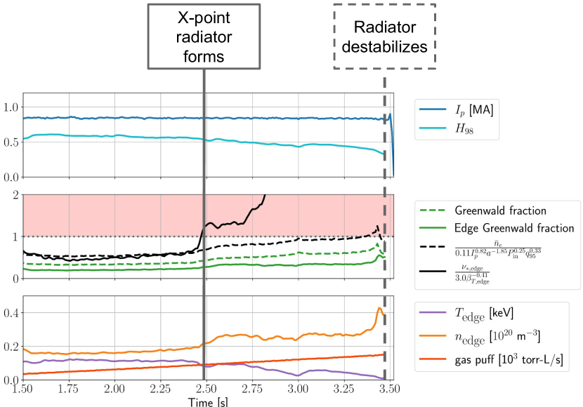
Figure 7: Time traces of DIII-D #191793, previously shown in Fig. 2, which ends in a major disruption. The middle panel shows the normalized instability score for four predictors: Greenwald fraction, edge Greenwald fraction, LSVM engineering boundary, and LSVM dimensionless boundary.

A false positive for the data-driven methods is shown in Fig. 8. This example is the most common failure case for Alcator C-Mod: transient EDA H-modes with low heating power. This incorrect classification may be due to the presence of the H-mode pedestal changing the correlation between the edge density and temperature (as defined in this study) with the separatrix density and temperature. If indeed the separatrix conditions set the density limit, once might expect failures when this correlation is broken.

From another perspective, this might not necessarily be a considered a failure at instability prediction, as the brief H-modes are not stable; while an LDL instability does not occur, H-to-L back-transition instabilities occur during both the excursions above the stability boundary, restoring the plasma state below the threshold after each return to L-mode. In general, other false positives can also occur for discharges with non-disruptive MARFEs or X-point radiators.

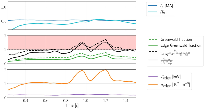
Figure 8: Time traces of non-disruptive C-Mod #1150806028, a low-auxiliary power discharge with two brief H-modes visible in the peaks in edge density around $t=0.9$s and $t=1.2$s.

4.5 Comparison of data-driven models

In each each of the three LDL prediction cases (engineering features, edge features, and dimensionless features), the NN, RF, and LSVM achieved comparable performances. This is especially true for the edge feature and dimensionless case, where the AUC and TNRs for these models are nearly indistinguishable. The linear regression approach, by contrast achieves notably worse performance in all cases. This illustrates two key points. The first is that a highly-parameterized ML architecture such as a NN or RF is not necessary for achieving high accuracy for predicting a specific instability when explanatory features are available. NNs and RFs are well suited for problems where simple, analytic functions cannot describe the observed behavior; in this case, we have sufficiently explanatory features to enable high performance from a power law.

The second point is that the approach to determining the power law makes a key difference. Classification via LSVM leads to far higher AUC and TNRs compared to linear regression in this study. This is not altogether surprising, as our goal is to distinguish LDL events from stable plasma states, and the classification method explicitly solves this problem. Linear regression has been commonly used for identifying density limit scalings, but this study suggests that a classification method like LSVMs may be more successful at finding a scaling to discriminate stable and unstable plasma states.

4.6 Limitations

We note that the number of discharges in our database from the five devices is not uniform, as shown in Tables 1 and 4. In particular, the large number of stable discharges from the C-Mod and DIII-D discharges give us good statistics for the TNR in the test set, but also means that the TNR is mostly determined by discharges on those two devices.

We also note there are strong correlations among $a$, $R_{0}$, and $B_{T}$ in our database (see A); it is therefore impossible to disentangle the independent causal effect of these three variables. Shaping variables $\epsilon$, $\kappa$, and $\delta$ are also not included in this analysis, as there is relatively little variance (standard deviation $\leq 25$% of the mean) across the dataset. Additionally, there are no negative triangularity discharges in this study.

The effect of isotope mass and impurities on the density limit are also not captured in this study. The database only contains deuterium majority density limit discharges, does not include effective charge $Z_{\rm eff}$ as a parameter, and excludes discharges where the operators noted a major impurity injection. The stability boundaries in this paper should therefore be applied only to relatively clean, hydrogenic discharges. It is worth emphasizing however, that the collisionality boundary works well on devices with carbon walls (DIII-D, TCV) as well as those with metal walls (AUG, C-Mod).

Many models for the density limit depend on the density and temperature at the separatrix, but we do not have these measurements across our database. We instead average over edge and temperature measurements from a relatively large “edge” region: $\rho=$ 0.85 to 0.95. While the density profile tends to be flat near the density limit, the temperature profiles do not. Nevertheless, we are able to achieve excellent LDL prediction with our definition of edge density and temperature.

4.7 Potential applicability for real-time control of burning plasmas

One of the key advantages of the LDL instability metrics identified in this study is that they can be used for real-time disruption prediction and plasma control. The most challenging measurements are the edge density and temperature signals computed from Thomson scattering (TS). While TS systems have low sampling rates relative to other diagnostics, such as the magnetics, TS measurements be frequent relative to the energy and particle confinement times that set the evolution rate of the temperature and density. For example, ITER edge TS ($r/a>0.85$) will have a temporal resolution of 10ms and spatial resolution of 5mm, compared to several seconds of energy confinement time and a 2.8m plasma minor radius [43].

Estimating the collisionality instability metric will be more challenging in fusion power plants (FPPs), as is the case for all sensing needs in FPPs. TS will likely be unavailable in FPPs because the large windows for gathering scattered photons conflict with tritium breeding requirements, but other diagnostics (reflectometers, interferometers, ECE) may be able to measure or enable the estimate of edge density and temperature.

In burning plasmas, however, edge collisionality will be very low due to the tremendous self-heating. Measuring the distance to the stability boundary in real time may only be necessary during the ramp-up and ramp-down phases.

5 Conclusion

In this multi-machine study, we leverage a manually labelled database to identify $\nu_{*,\rm edge}\beta_{T,\rm edge}^{0.4}=3$ as a reliable L-mode density limit stability boundary. This edge collisionality limit achieves excellent prediction performance (AUC = 0.996, TPR = 97.7% @ TPR = 95%), far outperforming Greenwald and edge Greenwald scalings. We are able to uncover this scaling by treating LDL prediction as a classification problem using a LSVM, not via linear regression. Other non-symbolic data-driven approaches, such as a NN and RF achieve similar accuracy as the LSVM power law.

The edge collisionality limit is reminiscent of the Greenwald limit in that it favors smaller devices with higher current (see eq. 8). However, we are only able to achieve high prediction accuracy by accounting for $T_{\rm edge}$ directly or through dimensionless quantities. We find that even when we search for a boundary in terms of engineering parameters, we find nearly the exact same dependencies as the edge collisionality, as shown by eq. 8. This limit appears to be consistent with observations the density limit correlating with electron adiabaticity $\alpha$ (eq. 10) and the formation of an X-point radiator, but we cannot confirm either association absent additional measurements of impurities and turbulent fluctuations.

This study also demonstrates the utility of LSVMs for identifying stability boundaries for specific events such as the LDL. For the edge and dimensionless features case, the LSVM identifies a power law with almost identical performance as the highly-parameterized NN and RF models. The LSVM power law also consistently outperforms the power law identified via linear regression. These results illustrate that for a specific instability and descriptive features, an LSVM can identify an accurate, analytic stability boundary.

This analysis is somewhat limited by non-uniform number of discharges available across devices and correlations among key parameters (ex. $a$, $R_{0}$, and $B_{T}$). Future work will seek to address these limitations by increasing the number of non-disruptive discharges from underrepresented machines in the database (AUG, TCV), expanding the database to new devices (JET), adding data from uncommon scenarios (DIII-D negative triangularity), and potentially including devices with other shapes and aspect ratios, such as spherical tokamaks.

We also discuss the potential applicability of the collisionality boundary as an instability metric for real-time control. Current experiments, such as DIII-D, and future experiments, such as ITER, have TS systems capable of measuring edge density and temperature at sufficiently high spatial and temporal resolution in real time. FPPs will face a more constrained sensing environment that preclude TS, but other diagnostics may be able to infer the relevant parameters. Additionally, the low collisionality in the edge of burning plasmas may obviate the need for density limit avoidance during the flattop. We will explore applying this indicator for real-time density limit avoidance in future work.

References

Appendix A Range of parameters in dataset

Table 7 shows the average value and standard deviation of macroscopic engineering parameters of the five devices in the database of this study. All parameters come from experiment measurements or equilibrium reconstructions except for the major radius of DIII-D and EAST, which are set as constant values (note: the major and minor radius of Alcator C-Mod have a finite but small standard deviation). The Pearson correlation matrix of several parameters used in this study are shown in Fig. 9.

Table 7: Average value and standard deviation of macroscopic parameters for each device in the database.

• Device	$n_{e}$ [$10^{20}$ m-3]	$I_{p}$ [MA]	$a$ [m]	$R_{0}$ [m]	$B_{T}$ [T]	$P_{\rm in}$ [MW]
  AUG	$0.68\pm 0.16$	$0.72\pm 0.13$	$0.50\pm 0.01$	$1.60\pm 0.01$	$2.41\pm 0.23$	$6.61\pm 1.66$
  C-Mod	$1.45\pm 0.68$	$0.83\pm 0.18$	$0.22\pm 0.00$	$0.68\pm 0.00$	$5.44\pm 0.81$	$1.73\pm 1.05$
  DIII-D	$0.44\pm 0.17$	$1.04\pm 0.21$	$0.59\pm 0.02$	$1.67\pm 0.00$	$1.94\pm 0.17$	$5.87\pm 3.17$
  EAST	$0.33\pm 0.09$	$0.35\pm 0.06$	$0.44\pm 0.01$	$1.83\pm 0.00$	$2.43\pm 0.00$	$3.29\pm 1.77$
  TCV	$0.47\pm 0.20$	$0.18\pm 0.07$	$0.23\pm 0.01$	$0.88\pm 0.01$	$1.42\pm 0.03$	$0.57\pm 0.49$

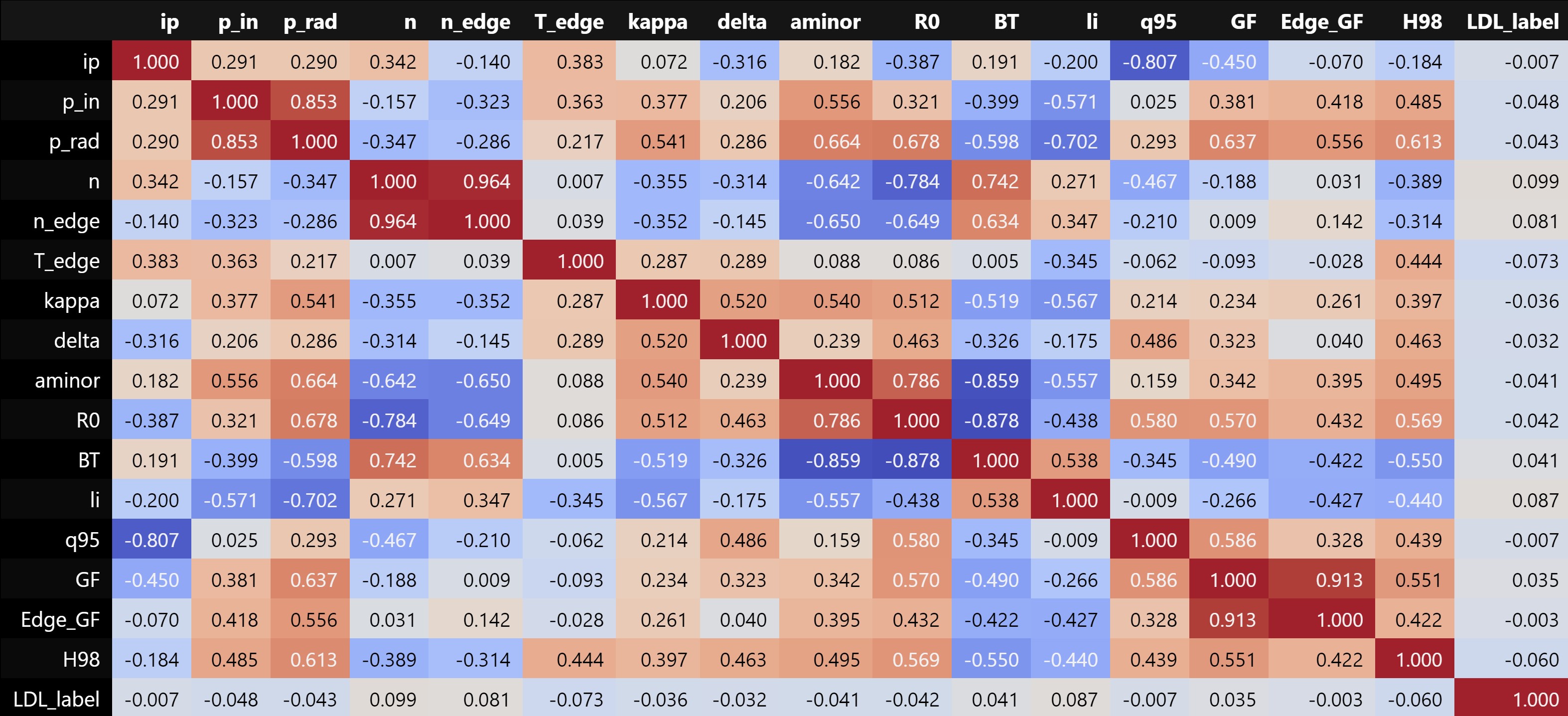
Figure 9: Correlation of several parameters utilized in this study across the entire dataset. “GF” is shorthand for Greenwald fraction.

Appendix B Hyperparameter ranges

The neural network, random forest, and LSVM were trained over a range of hyperparameters reported in Tables 8, 9, and 10. The NN and RF hyperparameters were sampled randomly, while all three LSVM hyperparameters were evaluated in a grid scan. Several sample-weighting methods were also explored, with minimal consistent effect on the final models.

Table 8: The hyperparameter ranges utilized for training the neural network.

• Hyperparameter	Range or values	Sampling distribution
  Learning rate	0.001 - 0.2	log uniform
  Batch size	32, 64	uniform
  # epochs	10 - 800	log uniform
  # layers	1 - 5	uniform
  # hidden units	16, 32, 64, 128	uniform
  drop out proportion	0 - 0.5	uniform
  activation function	relu, sigmoid	uniform

Table 9: The hyperparameter ranges utilized for training the random forest.

• Hyperparameter	Range or values	Sampling distribution
  # estimators	10, 30, 100	uniform
  max # features	3 - 8	uniform
  max depth	3, 5, 8	uniform
  min # samples per split	2, 5, 10	uniform
  min # samples per leaf	1, 2, 5, 10	uniform

Table 10: The hyperparameter ranges utilized for training the LSVM.

• Hyperparameter	Range or values	Sampling distribution
  C	0.1, 1, 10	uniform

Appendix C Generalizing to an unseen device

As long as fusion remains an experimental science, data-driven disruption predictors must be robust to “domain shifts,” i.e. differences between the training set and the cases observed during deployment. The best disruption prediction performances reported in the literature often from highly expressive machine learning architectures, such as neural networks and random forests, which can be especially vulnerable to domain shifts. Given the potentially catastrophic consequences of disruptions during a full-power discharge on ITER [33], robustness to domain shifts is a critical question for disruption prediction today.

We evaluate the robustness of our data-driven methods to an example of a domain shift: training on all AUG, C-Mod, and TCV discharges and then testing on DIII-D discharges. We utilize the dimensionless variables as in section 3.3, and therefore EAST is excluded due to lack of edge density and temperature measurements.

DIII-D was chosen for the test set because it has the largest current, major radius, and minor radius of devices in the database that includes edge measurements.

Table 11: The test set performance of LDL prediction for models trained on the edge features of AUG, C-Mod, and TCV but evaluated on DIII-D. The perfromance of the Greenwald fraction and Edge Greenwald fraction is also reported.

• Model	Analytic boundary	AUC	TNR @ TPR = 95%
  NN	N/A	0.986	94.4%
  RF	N/A	0.957	89.7%
  LSVM	$\nu_{*\rm,edge}^{\rm limit}\sim$ const.	0.989	98.0%
  Lin. Reg.	$\nu_{*\rm,edge}^{\rm limit}\beta_{T,\rm edge}^{-1.06}$	0.974	90.4%
  Greenwald	$\bar{n}^{\rm limit}\sim\frac{I_{p}}{\pi a^{2}}$	0.845	46.7%
  Edge Greenwald	$n_{\rm edge}^{\rm limit}\sim\frac{I_{p}}{\pi a^{2}}$	0.706	17.6%

The results are shown in Table 11. The LSVM and NN achieved the highest performance of all, with the LSVM being a simple boundary only in terms of the edge collisionality. The AUC is slightly degraded compared to when these parameters were fit on all machine (subsection 3.3), but both the NN and LSVM have TNR $>$ 94% @ TPR = 95%. The next best model is the linear regression model, followed by the RF. All data-driven models have better performance than the Greenwald scaling, despite the domain shift.

Appendix D Assessing Giacomin et al. [19] scaling as a disruption predictor on AUG, DIII-D, and TCV

Several theoretical models for the density limit, such as in Ref. [19], offer competing explanations of the density limit. As pointed out in Ref. [22], many of these recent studies have qualitative agreement in terms of power and current scalings. These theoretically-derived scalings are not explicitly intended for providing a warning to the density limit, but they could be used for this purpose. We therefore evaluate one proposed scaling for the maximum density from Ref. [19] to see how the scaling fairs as a LDL predictor.

To do so, we must rely on only AUG, DIII-D, and TCV, where we have consistent measurements of the power through the SOL. Additionally, we note that the scaling in Ref. [19] estimates the maximum density “in the proximity of the separatrix,” not the “edge” as we define it here (average between $\rho=0.85$ and $\rho=0.95$). The authors in Ref. [19] utilize this definition of edge density to provide supporting evidence the model, but we emphasize that we are not attempting to validate this model in this exercise. Our analysis overlaps in terms of AUG and TCV, but out study has data from DIII-D instead of JET and explicitly determines the accuracy of the metric in terms of LDL prediction.

In Table 12, we show the results of LDL prediction accuracy for a NN, RF, LSVM, linear regression model, the Greenwald fraction, the edge Greenwald fraction, and the Giacomin scaling. We see that the Giacomin scaling achieves higher AUC and TNR @ TPR = 95% than the Greenwald fractions. Compared with the data-driven models, however, the Giacomin scaling has a signficantly lower performance. The LSVM boundary achieves the highest AUC and matches the RF for highest TNR @ TPR = 95%. The LSVM boundary is nearly the same as the case presented earlier in section 3.3.

Table 12: The test set performance of LDL prediction for models trained and tested on dimensionless features for AUG, TCV, and DIII-D to compare of the Giacomin scaling [19]. The performance of the Greenwald fraction and Edge Greenwald fraction is also reported.

• Model	Analytic boundary	AUC	TNR @ TPR = 95%
  NN	N/A	0.987	94.6%
  RF	N/A	0.990	96.5%
  LSVM	$\nu_{*\rm,edge}^{\rm limit}\sim\beta_{T,\rm edge}^{-0.43}$	0.992	96.5%
  Lin. Reg.	$\nu_{*\rm,edge}^{\rm limit}\sim\beta_{T,\rm edge}^{-1.14}$	0.976	88.6%
  Giacomin	$n^{\rm limit}_{\rm edge}\sim\frac{I_{p}^{22/21}}{a^{79/42}}\frac{P_{SOL}^{10/21}A^{1/6}R_{0}^{1/42}}{B_{T}^{8/21}(1+\kappa^{2})^{1/3}}$	0.915	77.2%
  Greenwald	$\bar{n}^{\rm limit}\sim\frac{I_{p}}{\pi a^{2}}$	0.895	55.9%
  Edge Greenwald	$n_{\rm edge}^{\rm limit}\sim\frac{I_{p}}{\pi a^{2}}$	0.745	20.8%

Again, we emphasize that this is not an attempted validation of the Giacomin scaling, as we do not utilize the density at the separatrix to conduct this analysis. Our focus is to analyze the scaling as a method of forecasting the LDL given readily available measurements. On this count, it improves upon the Greenwald limit, but is not as reliable as the collisionality scaling.

References

- [1] J Rand McNally. The ignition parameter tn and the energy multiplication factor k for fusioning plasmas. Nuclear Fusion, 17(6):1273, 1977.
- [2] RJ Buttery, JM Park, JT McClenaghan, D Weisberg, J Canik, J Ferron, A Garofalo, CT Holcomb, J Leuer, PB Snyder, et al. The advanced tokamak path to a compact net electric fusion pilot plant. Nuclear Fusion, 61(4):046028, 2021.
- [3] SI Krasheninnikov, AS Kukushkin, and AA Pshenov. Divertor plasma detachment. Physics of Plasmas, 23(5), 2016.
- [4] Masanori Murakami, JD Callen, and LA Berry. Some observations on maximum densities in tokamak experiments. Nuclear Fusion, 16:347, 1976.
- [5] SJ Fielding, J Hugill, GM McCracken, JWM Paul, R Prentice, and PE Stott. High-density discharges with gettered torus walls in dite. Nuclear Fusion, 17:1382–1385, 1977.
- [6] Martin Greenwald. Density limits in toroidal plasmas. Plasma Physics and Controlled Fusion, 44(8):R27, 2002.
- [7] Martin Greenwald, JL Terry, SM Wolfe, S Ejima, MG Bell, SM Kaye, and GH Neilson. A new look at density limits in tokamaks. Nuclear Fusion, 28(12):2199, 1988.
- [8] M Shimada, DJ Campbell, V Mukhovatov, M Fujiwara, N Kirneva, K Lackner, MPVD Nagami, VD Pustovitov, N Uckan, J Wesley, et al. Overview and summary. Nuclear Fusion, 47(6):S1, 2007.
- [9] G Giruzzi, JF Artaud, Matteo Baruzzo, Tommaso Bolzonella, E Fable, L Garzotti, I Ivanova-Stanik, R Kemp, DB King, M Schneider, et al. Modelling of pulsed and steady-state demo scenarios. Nuclear Fusion, 55(7):073002, 2015.
- [10] BN Sorbom, J Ball, TR Palmer, FJ Mangiarotti, JM Sierchio, P Bonoli, C Kasten, DA Sutherland, HS Barnard, CB Haakonsen, et al. Arc: A compact, high-field, fusion nuclear science facility and demonstration power plant with demountable magnets. Fusion Engineering and Design, 100:378–405, 2015.
- [11] Andrew D Maris, Allen Wang, Cristina Rea, Robert Granetz, and Earl Marmar. The impact of disruptions on the economics of a tokamak power plant. Fusion Science and Technology, pages 1–17, 2023.
- [12] B LaBombard, RL Boivin, M Greenwald, J Hughes, B Lipschultz, D Mossessian, CS Pitcher, JL Terry, SJ Zweben, and Alcator Group. Particle transport in the scrape-off layer and its relationship to discharge density limit in alcator c-mod. Physics of Plasmas, 8(5):2107–2117, 2001.
- [13] Peng Shi, Ge Zhuang, K Gentle, Qiming Hu, Jie Chen, Qiang Li, Yang Liu, Li Gao, Xiaolong Zhang, Hai Liu, et al. First time observation of local current shrinkage during the marfe behavior on the j-text tokamak. Nuclear Fusion, 57(11):116052, 2017.
- [14] Xin Li, Shouxin Wang, Yuqi Chu, Hui Lian, Yinxian Jie, Rongjie Zhu, Yi Yuan, Liqing Xu, Tonghui Shi, Ang Ti, et al. Local current shrinkage induced by the marfe in l mode discharges on east tokamak. AIP Advances, 13(3), 2023.
- [15] B Lipschultz, B LaBombard, ES Marmar, MM Pickrell, JL Terry, R Watterson, and SM Wolfe. Marfe: an edge plasma phenomenon. Nuclear Fusion, 24(8):977, 1984.
- [16] U Stroth, M Bernert, D Brida, M Cavedon, R Dux, E Huett, T Lunt, O Pan, M Wischmeier, the ASDEX Upgrade Team, et al. Model for access and stability of the x-point radiator and the threshold for marfes in tokamak plasmas. Nuclear Fusion, 62(7):076008, 2022.
- [17] Paolo Zanca, F Sattin, DF Escande, and JET Contributors. A power-balance model of the density limit in fusion plasmas: application to the l-mode tokamak. Nuclear fusion, 59(12):126011, 2019.
- [18] BN Rogers, JF Drake, and A Zeiler. Phase space of tokamak edge turbulence, the l- h transition, and the formation of the edge pedestal. Physical Review Letters, 81(20):4396, 1998.
- [19] M Giacomin, A Pau, P Ricci, O Sauter, T Eich, JET Contributors, ASDEX Upgrade Team, et al. First-principles density limit scaling in tokamaks based on edge turbulent transport and implications for iter. Physical Review Letters, 128(18):185003, 2022.
- [20] Thomas Eich, Peter Manz, ASDEX Upgrade Team, et al. The separatrix operational space of asdex upgrade due to interchange-drift-alfvén turbulence. Nuclear Fusion, 61(8):086017, 2021.
- [21] Rameswar Singh and PH Diamond. Zonal shear layer collapse and the power scaling of the density limit: old lh wine in new bottles. Plasma Physics and Controlled Fusion, 64(8):084004, 2022.
- [22] Peter Manz, Thomas Eich, and Ondrej Grover. The power dependence of the maximum achievable h-mode and (disruptive) l-mode separatrix density in asdex upgrade. Nuclear Fusion, 2023.
- [23] A Gibson. Fusion relevant performance in jet. Plasma Physics and Controlled Fusion, 32(11):1083, 1990.
- [24] Y Kamada, N Hosogane, R Yoshino, T Hirayama, and T Tsunematsu. Study of the density limit with pellet fuelling in jt-60. Nuclear fusion, 31(10):1827, 1991.
- [25] A Stabler, K McCormick, V Mertens, ER Muller, J Neuhauser, H Niedermeyer, K-H Steuer, H Zohm, F Dollinger, A Eberhagen, et al. Density limit investigations on asdex. Nuclear fusion, 32(9):1557, 1992.
- [26] TH Osborne, AW Leonard, MA Mahdavi, M Chu, ME Fenstermacher, R La Haye, G McKee, TW Petrie, E Doyle, G Staebler, et al. Gas puff fueled h-mode discharges with good energy confinement above the greenwald density limit on diii-d. Physics of Plasmas, 8(5):2017–2022, 2001.
- [27] G Pucella, O D’Arcangelo, O Tudisco, F Belli, W Bin, A Botrugno, P Buratti, G Calabrò, B Esposito, E Giovannozzi, et al. Analytical relation between peripheral and central density limit on ftu. Plasma Physics and Controlled Fusion, 59(8):085011, 2017.
- [28] C Angioni, H Weisen, OJWF Kardaun, M Maslov, A Zabolotsky, C Fuchs, L Garzotti, C Giroud, B Kurzan, P Mantica, et al. Scaling of density peaking in h-mode plasmas based on a combined database of aug and jet observations. Nuclear Fusion, 47(9):1326, 2007.
- [29] G Duesing. First results of neutral beam heating on jet. Plasma Physics and Controlled Fusion, 28(9A):1429, 1986.
- [30] J Rapp, PC De Vries, FC Schüller, W Biel, R Jaspers, HR Koslowski, A Krämer-Flecken, A Kreter, M Lehnen, A Pospieszczyk, et al. Density limits in textor-94 auxiliary heated discharges. Nuclear Fusion, 39(6):765, 1999.
- [31] Alexander Huber, S Brezinsek, M Groth, PC De Vries, V Riccardo, G Van Rooij, G Sergienko, G Arnoux, A Boboc, P Bilkova, et al. Impact of the iter-like wall on divertor detachment and on the density limit in the jet tokamak. Journal of Nuclear Materials, 438:S139–S147, 2013.
- [32] M Bernert, T Eich, A Kallenbach, D Carralero, A Huber, PT Lang, S Potzel, F Reimold, J Schweinzer, E Viezzer, et al. The h-mode density limit in the full tungsten asdex upgrade tokamak. Plasma Physics and Controlled Fusion, 57(1):014038, 2014.
- [33] M. Lehnen, P. Aleynikov, and B. Bazylev. Plasma Disruption Management in ITER. 2018. Number: IAEA-CN–234.
- [34] Cristina Rea, RS Granetz, K Montes, Roy Alexander Tinguely, N Eidietis, Jeremy M Hanson, and B Sammuli. Disruption prediction investigations using machine learning tools on diii-d and alcator c-mod. Plasma Physics and Controlled Fusion, 60(8):084004, 2018.
- [35] Kevin Joseph Montes, Cristina Rea, RS Granetz, Roy Alexander Tinguely, N Eidietis, OM Meneghini, DL Chen, Biao Shen, BJ Xiao, Keith Erickson, et al. Machine learning for disruption warnings on alcator c-mod, diii-d, and east. Nuclear Fusion, 59(9):096015, 2019.
- [36] Wenhui Hu, Jilei Hou, Zhengping Luo, Yao Huang, Dalong Chen, Bingjia Xiao, Qiping Yuan, Yanmin Duan, Jiansheng Hu, Guizhong Zuo, et al. Prediction of multifaceted asymmetric radiation from the edge movement in density-limit disruptive plasmas on experimental advanced superconducting tokamak using random forest. Chinese Physics B, 32(7):075211, 2023.
- [37] Geert Verdoolaege, Stanley M Kaye, Clemente Angioni, Otto JWF Kardaun, Mikhail Maslov, Michele Romanelli, François Ryter, Knud Thomsen, JET Contributors, ASDEX Upgrade Team, et al. The updated itpa global h-mode confinement database: description and analysis. Nuclear Fusion, 61(7):076006, 2021.
- [38] PC De Vries, G Pautasso, D Humphreys, M Lehnen, S Maruyama, JA Snipes, A Vergara, and L Zabeo. Requirements for triggering the iter disruption mitigation system. Fusion Science and Technology, 69(2):471–484, 2016.
- [39] Peter C Stangeby et al. The plasma boundary of magnetic fusion devices, volume 224. Institute of Physics Pub. Philadelphia, Pennsylvania, 2000.
- [40] RJ Hajjar, PH Diamond, and MA Malkov. Dynamics of zonal shear collapse with hydrodynamic electrons. Physics of Plasmas, 25(6), 2018.
- [41] R Hong, GR Tynan, PH Diamond, L Nie, D Guo, T Long, R Ke, Y Wu, B Yuan, M Xu, et al. Edge shear flows and particle transport near the density limit of the hl-2a tokamak. Nuclear Fusion, 58(1):016041, 2017.
- [42] T Long, PH Diamond, R Ke, L Nie, M Xu, XY Zhang, BL Li, ZP Chen, X Xu, ZH Wang, et al. Enhanced particle transport events approaching the density limit of the j-text tokamak. Nuclear Fusion, 61(12):126066, 2021.
- [43] M Bassan, P Andrew, G Kurskiev, E Mukhin, T Hatae, G Vayakis, E Yatsuka, and M Walsh. Thomson scattering diagnostic systems in iter. Journal of Instrumentation, 11(01):C01052, 2016.