The -adic Jaynes-Cummings model in symplectic geometry
Abstract.
The notion of classical -adic integrable system on a -adic symplectic manifold was proposed by Voevodsky, Warren and the second author a decade ago in analogy with the real case. In the present paper we introduce and study, from the viewpoint of symplectic geometry and topology, the basic properties of the -adic version of the classical Jaynes-Cummings model. The Jaynes-Cummings model is a fundamental example of integrable system going back to the work of Jaynes and Cummings in the 1960s, and which applies to many physical situations, for instance in quantum optics and quantum information theory. Several of our results depend on the value of : the structure of the model depends on the class of the prime modulo and requires special treatment.
1. Introduction
Symplectic geometry is concerned with the study of symplectic manifolds, that is, smooth manifolds endowed with a closed non-degenerate -form. The subject has its roots in the study of planetary motions in the XVII and XVIII centuries, and has undergone extensive developments since then. We refer to [14, 26, 37, 43] for surveys on symplectic geometry which also mention historical developments.
Usually in symplectic geometry one works with smooth manifolds and differential forms over the real numbers, and there is a large body of work for this case. On the other hand, in this paper we are going to work with the case in which the field of real numbers is replaced by the field of -adic numbers , where is a fixed prime number. Recall that can be defined as a completion of with respect to a non-archimedean absolute value (as we will recall in Appendix A). In [29] V. Voevodsky, M. Warren and the second author gave a construction of from the point of view of homotopy type theory and Voevodsky’s Univalent Foundations. Their long-term goal was constructing the theory of -adic integrable systems on -adic symplectic manifolds, with an eye on eventually formalizing this theory using proof assistants. In [29, Section 7] the authors propose a notion of -adic integrable system and sketch a possible research program concerning these systems. We recommend [3, 33, 34] for a concise introduction to homotopy type theory and Voevodsky’s Univalent Axiom.
The present paper continues the work sketched by Pelayo, Voevodsky and Warren in [29, Section 7]. More precisely, we start to develop the basics of -adic integrable systems proposed therein, by focusing on working out the -adic analog of an integrable system of great importance: the classical Jaynes-Cummings model (Figure 1), also known in the mathematics community as the coupled spin-oscillator, because it comes from coupling an oscillator and a spin in a non-trivial way. It is a fundamental example of integrable system with two degrees of freedom. The Jaynes-Cummings model was originally introduced [21] to give a description of the interaction between an atom prepared in a mixed state with a quantum particle in an optical cavity. The Jaynes-Cummings model has been studied or applied in different contexts, and from several viewpoints, and is relevant across a number of areas within physics, chemistry and mathematics, the reason being that it represents the simplest possible way to have a finite dimensional state, like a spin, be in interaction with an oscillator. For instance, the model has been found to apply to physical situations in the contexts of quantum physics, quantum optics or quantum information theory [20, 35, 39]. It is also of high interest in mathematical physics, see for instance [4, 5, 6], and symplectic geometry [1, 24, 32].
Unlike in [29], in the present paper we use the more familiar non-constructive definition of , since the purpose of the current paper is to start developing the theory of -adic integrable systems, and it does not matter which definition of one uses. However, for problems involving the use of algorithms or constructive proofs one should use the construction of which is given in [29].
We believe that it is crucial to have at least an important example of -adic integrable system worked out in detail before trying to develop a general theory, hence this paper. The example of the Jaynes-Cummings model shows that a general theory will be subtle, yet worthwhile pursuing in our opinion. In particular, understanding this example requires combining techniques from symplectic geometry and -adic analysis and some of the conclusions were surprising to us. For instance, the structure of the system varies significantly depending on the class of the prime modulo , and the case of often requires a special treatment.
The following result, from the paper [32] by Vũ Ngọc and the second author, describes the basic properties of the classical “real” Jaynes-Cummings model.
Proposition 1.1 (Real Jaynes Cummings model [32, Prop. 2.1]).
The coupled spin-oscillator , defined by
with coordinates on and on and symplectic form , is an integrable system, meaning that the Poisson bracket vanishes everywhere.
In addition, the map is the momentum map for the Hamiltonian circle action of on that rotates simultaneously horizontally about the vertical axis on , and about the origin on .
The critical points of the coupled spin-oscillator are non-degenerate and of elliptic-elliptic, transversally-elliptic or focus-focus type. It has exactly one focus-focus singularity at the “North Pole” and one elliptic-elliptic singularity at the “South Pole” .
In the paper [32] the following information about the Jaynes-Cummings model was either also determined or it can be easily deduced from it (either from considerations in the paper or by general theory, which is not available to us in the -adic case):
All of these results have analogs if one replaces by the -adic sphere and by the -adic plane , while keeping the same formulas for and . These analogs are more complicated to formulate than in the real case and depend on the value of .
We refer to [9, 10, 11, 12] for works which deal with different geometric aspects of -adic geometry and mathematical physics, and to [18, 22, 38] for books on -adic numbers, -adic analysis, -adic manifolds, and related concepts.
Structure of the paper
The paper is organized as follows.
-
•
In Section 2 we state the main results of the paper.
-
•
In Section 3 we recall the notions of -adic symplectic manifold and -adic integrable system.
-
•
In Section 4 we analyze the structure of -adic circles, in order to calculate the image and fibers of the -adic oscillator.
-
•
In Section 5 we study the -adic spin system, and also calculate its image and fibers.
-
•
In Section 6 we start studying the coupling of both models (oscillator and spin).
-
•
In Section 7 we deduce the normal forms of the critical points of this coupling.
The paper concludes with three appendices in which we recall some facts we need and prove some technical results that are used in the main part of the paper. Concretely:
Acknowledgements
The first author is funded by grants PID2019-106188GB-I00 and PID2022-137283NB-C21 of MCIN/AEI/10.13039/501100011033 / FEDER, UE and by project CLaPPo (21.SI03.64658) of Universidad de Cantabria and Banco Santander.
The second author is funded by a BBVA (Bank Bilbao Vizcaya Argentaria) Foundation Grant for Scientific Research Projects with title From Integrability to Randomness in Symplectic and Quantum Geometry. He thanks the Dean of the School of Mathematics Antonio Brú and the Chair of the Department of Algebra, Geometry and Topology at the Complutense University of Madrid, Rutwig Campoamor, for their support and excellent resources he is being provided with to carry out the BBVA project.
We are very thankful to María Inés de Frutos, Antonio Díaz-Cano and Juan Ferrera for many helpful discussions and feedback on a preliminary version of this paper.
2. Main results
The following results describe the basic properties of the -adic Jaynes-Cummings model. In contrast with the real case and for reasons which will become clear later, we develop the theory of this system viewed as a -adic analytic map on a -adic analytic manifold, which is the situation for which we later give general definitions. Below the notation , where , refers to -adic order, that is, an integer such that
The concepts of critical point, rank of a critical point and non-degeneracy for a critical point which appear in the statement below are defined in the -adic case, via direct analogy with the real case. The concept of action of a -adic Lie group is defined in Appendix C. Finally, the -adic analog of the circle , and in general the -sphere for , is the -adic -sphere, which is defined as
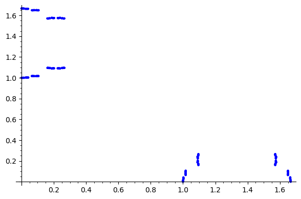
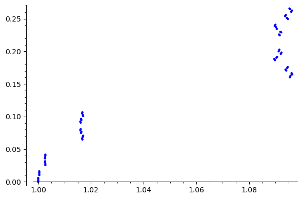
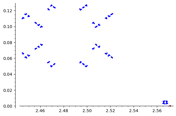
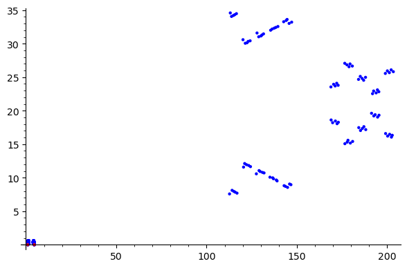
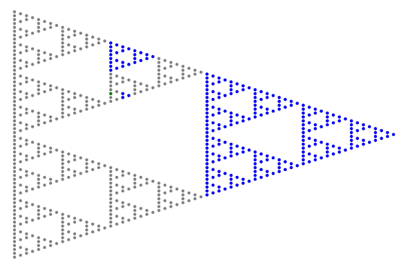
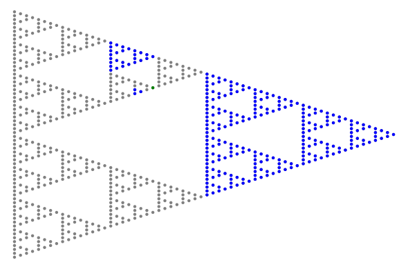
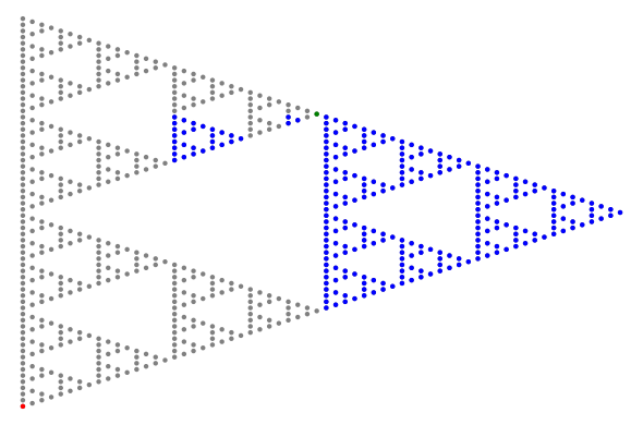
We refer to Figure 3 for an illustration of the following result when .
Theorem 2.1 (Classical spectrum and critical points of -adic Jaynes-Cummings model).
Let be a prime number. Let be the -adic Jaynes-Cummings model, that is, the -adic analytic map given by
where , and is endowed with the -adic analytic symplectic form , where are angle-height coordinates on . Then the following statements hold.
-
(1)
The map is a -adic analytic integrable system, that is, (Theorem 6.2).
-
(2)
The map is the momentum map of the Hamiltonian action of that rotates simultaneously horizontally about the vertical axis on , and about the origin on (Theorem 6.2(1)).
- (3)
-
(4)
The set of critical points of is given as follows (Theorem 6.2(2)).
-
(a)
the set of rank points is .
-
(b)
the set of rank points is
-
(a)
Remark 2.2.
In part (3b) of the previous theorem, we use “contains” because we do not have a complete description of the image of the system for . Deciding whether some points are in the image seems more complicated than for other primes, partly because is compact while is not compact for any other .
The following is the most interesting result of the paper, and the one for which the calculations are more involved. A depiction of this result is given in Figure 3.
Theorem 2.3 (Fibers of -adic Jaynes-Cummings model).
Let be a prime number. Let be the -adic Jaynes-Cummings model, that is, the -adic analytic map given by
where , and is endowed with the -adic analytic symplectic form , where are angle-height coordinates on . The fibers of are given as follows.
-
(1)
Suppose that (Theorems 6.11 and 6.19).
-
(a)
If , then the fiber is the disjoint union of a -dimensional -adic analytic submanifold, which may be empty depending on the value of , and an isolated point at .
-
(b)
If , then the fiber has dimension and a singularity at . (By this we mean that minus the critical point is a -adic analytic submanifold of dimension , but as a whole it is not a manifold because it has a singularity at the critical point, as happens in the real case for the same point, as in Figure 2).
-
(c)
If is a rank critical value, that is, and for some such that is the sum of two squares, then the following statements hold.
-
(i)
If is a non-square modulo , the fiber is the disjoint union of a -dimensional -adic analytic submanifold and the -dimensional -adic analytic submanifold homeomorphic to which consists exactly of the critical points whose image is .
-
(ii)
If is a square modulo , the fiber has dimension and singularities at the critical points. (By this we mean, as in case (b), that minus the set of critical points is a -adic analytic submanifold of dimension , but as a whole it has singularities at the critical points contained in . In the real case this only happens for the pinched torus in Figure 2.)
-
(i)
-
(d)
For the rest of values of , the fiber is a -dimensional -adic analytic submanifold.
-
(a)
-
(2)
Suppose that (Theorem 6.12).
-
(a)
If is a rank critical value, the fiber has dimension and a singularity at every point of , where
-
(b)
Otherwise, has the same form as in part (1).
-
(a)
Remark 2.4.
We conclude this introduction discussing the local models of the -adic Jaynes-Cummings model at the critical points. In this case the computations are analogous to the real case, and roughly speaking so are the conclusions, although some simplifications of the expressions below can be given in the real case, as we see later (Corollary 7.3).
Proposition 2.5 (Normal forms at critical points of -adic Jaynes-Cummings model).
All critical points in part (4) of Theorem 2.1 are non-degenerate and their local normal forms are given as follows.
-
(1)
At , there are local coordinates such that the -adic symplectic form is given by and
Here with
We say that is a point of “elliptic-elliptic” type (Proposition 7.6).
-
(2)
At , there are local coordinates such that the -adic symplectic form is given by and
Here with
We say that is a point of “focus-focus” type (Proposition 7.8).
-
(3)
Let be the -adic analytic functions given by . Then, at any rank point , there are local coordinates such that the -adic symplectic form is given by and
Here with
We say that any of the points is a point of “transversally elliptic” type (Proposition 7.2). Recall that these points were defined in Theorem 2.1(4).
Remark 2.6.
In principle the local models in Proposition 2.5 do not depend on the value of , but of course some further simplifications are possible for some values of . However the “type” of the point (elliptic-elliptic, etc.) does not change.
| -adic | ||||
| Real | ||||
| Image of Hamiltonians | green region in Figure 2 | no easy description | all | all |
| Fiber of regular value | dimension analytic manifold (isomorphic to a torus) | dimension analytic manifold (not isomorphic to a torus) | ||
| Fiber of rank value ( not square) | circle | circle + dimension analytic manifold | ||
| Fiber of rank value ( square) | never happens | never happens | dimension , singular at a circle | |
| Fiber of | point | point | dimension , singular at four lines | point + dimension analytic manifold |
| Fiber of | dimension , singular at a point | dimension , singular at a point | dimension , singular at four lines | dimension , singular at a point |
Table 1 summarizes the results of Theorems 2.1 and 2.3. Figure 3 gives an idea of what the critical points look like in the -adic case. The richness which this simple example exhibits is an indication that a general -adic theory of integrable systems will include many intricacies.
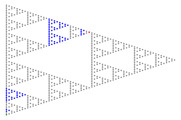
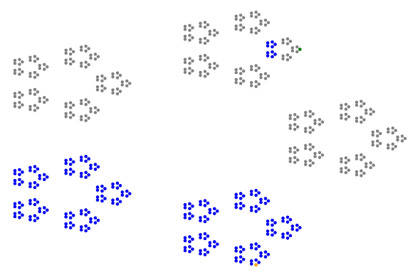
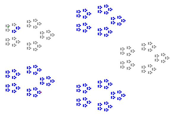
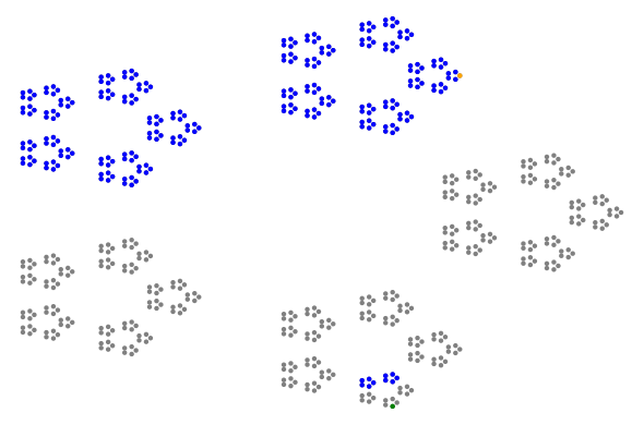
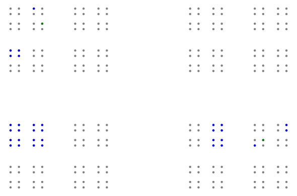
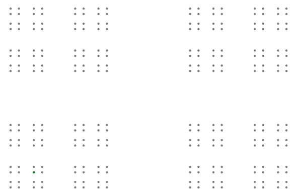
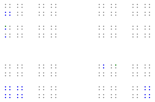
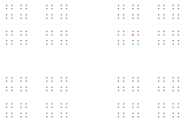
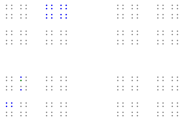
In this article when we discuss images and fibers of functions, we will frequently graphically represent our findings. This is a problem because we are working with the -adic field, and representations are usually done with real values. The solution is to “translate” the -adic numbers into real ones.
We will use two types of representations, which we will call -dimensional and -dimensional. In the -dimensional ones, only one variable is to be represented: suppose it is . We choose a map
from the values of to complex numbers and represent them as such (in the usual way where is represented as ). The mapping is chosen so that the distance between and represents the distance between and in the most accurate possible way. The solution we have found, which is not the only one possible, is as follows:
-
•
If ,
-
•
If ,
-
•
If ,
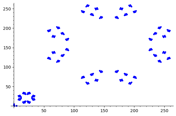
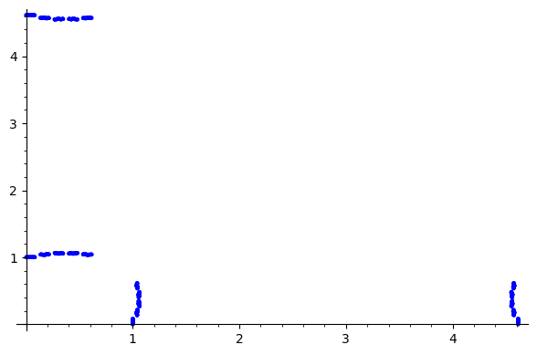
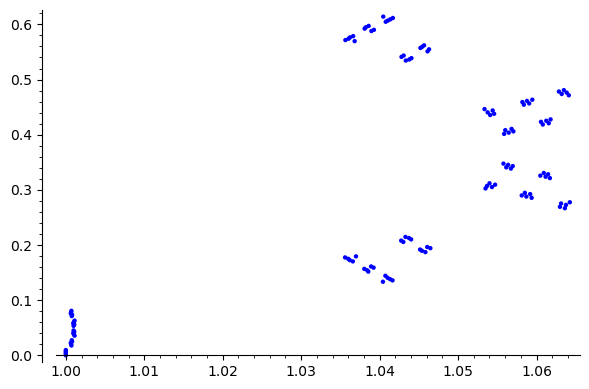
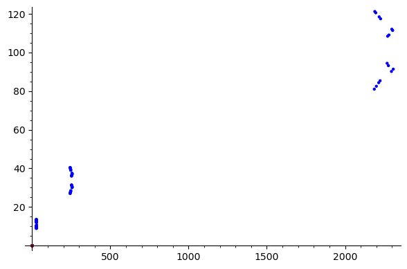
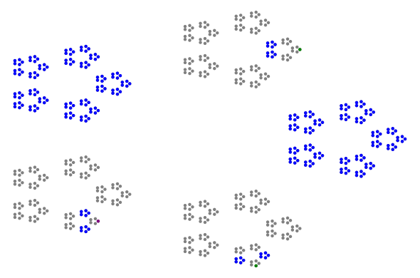
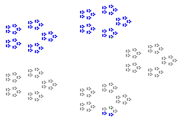
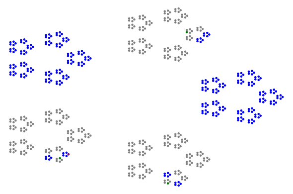
Examples of these representations can be seen in Figures 11, 12 and 13, for the different primes. For example, in Figure 12 we can see a pentagon divided in five pentagons. Each one of these five pentagons represents a remainder modulo (hence, a -adic ball of radius ). They are in turn subdivided in five pentagons, which represents balls of radius , and so on.
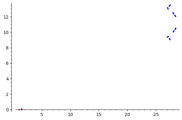
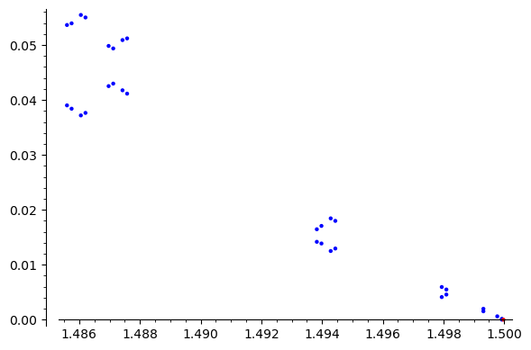
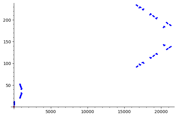
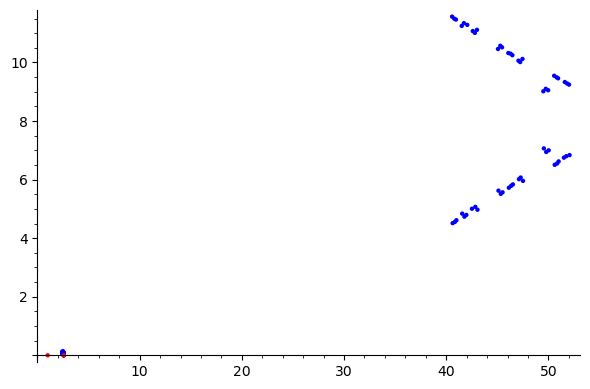
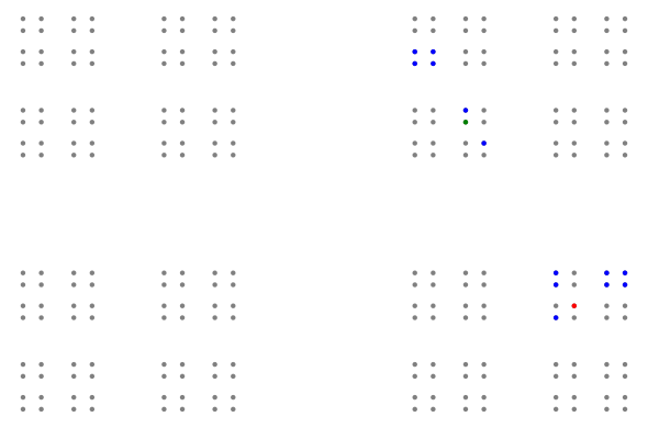
The -dimensional representations are recognized by their coordinate axes. Here two variables are being represented, say and . A point is mapped to by applying componentwise the correspondence
where for , for , and for . For example, in Figure 14 of the Appendix A, we are representing a function from to ; is the independent variable and is the dependent one. The five clusters in which the points are divided correspond to -adic balls of radius when projected to the -axis. They can be seen, in turn, subdivided into five clusters, which correspond to being in a ball of radius , and so on. The same clusters occur in the -axis. The values in the axes do not represent -adic numbers, but the real numbers resulting from the mapping.
All figures in this paper, including the -adic representations, have been done using computer code developed in Sage.
3. -adic analytic integrable systems
In this section we review the basic notions of -adic symplectic geometry when the field of coefficients is replaced by the field of -adic numbers . These extensions were proposed in an earlier paper by Pelayo, Voevodsky and Warren [29, Section 7] in 2015.
3.1. -adic analytic manifolds
First we review some concepts for -adic differential geometry, which can be found in the literature (see for example [38]), starting with the concept of a -adic manifold. The following definitions are straightforward extensions of the real case. Following [38, Sections 7-8], given a Hausdorff topological space and an integer , an -dimensional -adic analytic atlas is a set of functions , where and are open subsets, such that
-
•
is a homeomorphism between and ;
-
•
for any , the change of charts is bi-analytic, i.e. it is analytic with analytic inverse.
Such an together with such an atlas is called an -dimensional -adic analytic manifold. A maximal atlas for has a chart for each open set. The integer is called the dimension of .
Now let and be -adic analytic manifolds of dimensions and respectively, a map is analytic if, for any , there are neighborhoods of and of such that is analytic (as a function from a subset of to a subset of ). is bi-analytic, or an isomorphism of -adic analytic manifolds, if it is bijective and and are analytic.
Theorem 3.1 ([38, Proposition 8.6]).
Let be a prime number. For a -adic analytic manifold the following conditions are equivalent.
-
(1)
is paracompact (any open covering can be refined to a locally finite one).
-
(2)
is strictly paracompact (any open covering can be refined to one consisting in pairwise disjoint sets).
-
(3)
is an ultrametric space (its topology can be defined by a metric that satisfies the strict triangle inequality).
Corollary 3.2.
Let be a prime number. Any paracompact -adic analytic manifold is isomorphic to a disjoint union of -adic analytic balls. Hence, a compact -adic analytic manifold is isomorphic to a finite disjoint union of -adic analytic balls.
Corollary 3.2 implies that, when defining an atlas for a manifold, we can take the open sets in the atlas as disjoint, and the charts sending them to balls in .
The last part of Corollary 3.2 was strengthened by Serre [40]: two finite disjoint unions of balls are isomorphic if and only if the corresponding numbers of balls differ by a multiple of . That is, there are exactly compact -adic manifolds, modulo isomorphism.
The notions of -adic analytic function, -adic vector field and -adic differential form are analogous to the ones in the real case. In order to make the paper as accessible as possible and make some elementary comparisons with the real case, we review these notions in Appendix B.
3.2. -adic integrable systems
Let be a prime number. A -adic analytic symplectic manifold is a pair where is a -adic analytic manifold and is a closed non-degenerate analytic -form in . For example, if is a -adic analytic manifold, then the canonical symplectic form on is also analytic by construction.
Given a -adic analytic symplectic manifold and a -adic analytic function , there is a unique -adic analytic vector field that satisfies
| (3.1) |
As in the real case, is called the Hamiltonian vector field associated to . We recall the proof of this fact, which is the same as in the real case. Let . We may assume that has the form
in coordinates near , and . Hence .
Also as in the real case, the Poisson bracket of two -adic analytic functions is defined by
Definition 3.3 (Pelayo-Voevodsky-Warren [29, Definition 7.1]).
Let be a prime number and let be a -adic analytic symplectic manifold. We say that a -adic analytic map
is a -adic analytic integrable system if two conditions hold:
-
(1)
The functions satisfy for all ;
-
(2)
The set where the differential -forms are linearly dependent has -adic measure zero.
In item (2) of Definition 3.3 the -adic measure is with respect to the -adic volume form .
Throughout the paper, whenever we speak of analytic maps we always mean -adic analytic maps, and similarly for manifolds.
4. The -adic analytic oscillator on
This section starts the main part of the paper. Recall that our goal is to start developing the theory of -adic integrable systems, so we will start with the simplest example, which is the oscillator, that is, the system
with Hamiltonian
on endowed with the standard -adic symplectic form . Since this section we believe is interesting in its own right, independently on the upcoming sections, we use for the variables on , instead of , because it is more common.
As it is well known, in the real case the trajectory in the phase space of this system coincides with the fiber of , which is a circle. In the -adic case, we will see that the trajectory is part of the fiber of . Actually, is the momentum map of a -adic circle action (see Definition C.3). This will be useful later because the oscillator is used in the construction of the Jaynes-Cummings model.
As the fiber of is a circle, we will first find some structure in and other circles in the -adic plane , to which we dedicate Section 4.1. Then in Section 4.2 we study the -adic harmonic oscillator.
We refer to Appendix A for the basic definitions concerning the -adic numbers, which we use below.
4.1. The structure of -adic analytic circles
We can understand a point in as acting on (in the sense of Appendix C) as multiplication by the matrix
These matrices are called unitary in real symplectic algebra, due to its identification with complex numbers of absolute value that associates to this matrix the number . In -adic algebra, this identification does not make much sense because not all complex -adics can be expressed as , for ; actually some of them are transcendental over (the field is not defined as the algebraic closure of , but as the metric completion of that closure). This means that the identification will not be surjective.
Despite of this, we will still call these matrices unitary because it is not clear what this term should mean in the complex -adic context. (A unitary matrix in is a matrix such that . This definition uses the notion of complex conjugate, which has no canonical equivalent in because the Galois group of the extension is infinite.)
Let , where . In the real case, given two points , for , there is a unitary matrix that sends one point to the other:
| (4.1) |
Also, all unitary matrices have the form
| (4.2) |
In terms of Lie groups, this is to say that the group of unitary matrices is the same as the group of rotation matrices, which is essentially , because the domain of the functions is and their values repeat with period .
Now we turn to the -adic case. The group of rotation matrices can now be identified with , where if and otherwise , because this is the domain of the cosine and the sine, and the latter is injective as a function from to (see Appendix A). We will see now that this group does not coincide with , but instead it is a proper subgroup. Equivalently, the set of points of the form for , does not give all the points in .
Proposition 4.1.
Let be a prime number. Let be given by . Let and (concretely, if ). Then the following statements hold.
-
(i)
Any two points in are related by the action of , except if , in which case only proportional points are related.
-
(ii)
Two points are related by a rotation matrix if and only if
(4.3) where
and if and otherwise .
This , that is constant in an orbit of , will be called the order of the orbit.
Proof.
We start with the “degenerate case” . If or , the only solution to is and , so suppose .
Now
where is an element of such that . Let and be two elements in with . If there is a unitary matrix which sends one to the other, we have
and
which implies . For the other direction, if , the matrix
is unitary and sends to . This shows part (i).
In order to prove part (ii), we need the matrix to be a rotation matrix. This happens when
This needs that , which implies
as we wanted.
Now we turn to . The unitary matrix for part (i) is the same matrix (4.1) as in the real case. For part (ii), this matrix is a rotation matrix if and only if
| (4.4) |
for some .
By changing to
we may assume that . Now, the first four numbers are in , but not all of them in . Without loss of generality, suppose . Let . The conditions (4.3) are now written as
| (4.5) | ||||
| (4.6) |
Now make the change , where (because ):
| (4.7) | ||||
| (4.8) |
As , (4.8) solves as . Substituting in (4.7), we get
But we also know that
and together with the previous equation
and
as we wanted.
Conversely, suppose that (4.5) and (4.6) hold. We know that , and by (4.5), also . Let and . We have that
and the same for . Using (4.5) we get
which implies , that is
(the exponent of is always the same unless , in which case it goes one up when squaring and one down when canceling the squares, as in Corollary A.6). We claim that the plus sign holds.
By (4.6),
so we must have . If , the claim is proved. Otherwise, is a multiple of , which implies is not and . So the minus sign cannot hold, and the claim is proved.
Now
It follows from Proposition A.11 that is in the image of the sine series, so there is such that . This implies
and
Moreover,
so the plus sign must hold, and and are related by a rotation. ∎
Proposition 4.2.
Let be a prime number. Let be given by . Let and let and (concretely, if ). Given , the number of order orbits of the rotation group in is given as follows.
-
•
If :
-
•
If :
-
•
If :
Proof.
As before, we start with the case (and ). If or , is empty and the number of orbits is zero. Otherwise, an orbit is
for fixed and with , with the order determined by the order of . Two choices of give different orbits if and only if their leading digits differ, which gives orbits ( values of times leading digits of ).
Now we turn to . Without loss of generality, we take (otherwise change to ).
We start with . Let be the set of orbits and be the set of pairs such that , where is the finite field of order . Of course, and are empty if .
By Proposition 4.1, there is an injective correspondence
that assigns to the orbit of the pair . For the case , is surjective, because if we have with we can lift them to (apply Theorem A.5).
Suppose that . must satisfy , and and are not both . This means , which has no solution if and leaves two possible values for otherwise. For each of these solutions, and can take possible values, and we are done.
Now let us assume that . This means that , and must satisfy .
-
•
If , there is such that and
(4.9) Substituting in (4.9),
which, for a fixed value of , has one solution for , and in turn one solution for . Moreover, the same cannot be obtained for two values of , hence there are as many solutions as values for , which are .
-
•
If , is irreducible modulo , so it has a root in such that generates as a -vector space. Defining as usual the conjugate of as for , we can write
and the problem reduces to count the number of such that . Let be the set of such . We have that:
-
–
;
-
–
If and ,
and ;
-
–
is not empty: if is a square modulo , this is obvious. Otherwise, let be the smallest non-square modulo and . By our choice of , for some , and
which implies .
This together implies that, for , is a bijection between and , which implies that all the have the same size and
as we wanted.
-
–
-
•
If , we suppose without loss of generality that is odd. Consider first the case where is even. In this case , so the other case () has no solution. We need to choose and . will always be , and can be or . Hence (which is or ) determines , and can be chosen freely between and . Once we have and so that , we can fix and lift using Corollary A.6. This leaves two orbits, and the other two come from swapping and .
In the other case, and are both odd and . This means that the cases and have no solution. We can choose four possibilities for and modulo . Again, Corollary A.6 allows us to lift this to four orbits for and .
∎
Corollary 4.3.
Let be given by . Let in and let .
-
•
If and , consists of orbits for the rotation group with each order , together with orbits with order if is even. The set consists of two lines, that form orbits with each integer order and one with their intersection point .
-
•
If and , is empty if is odd, and otherwise consists of orbits, all with order . The set is a single point.
-
•
If and , consists of orbits with order , if it is not empty. The set is again a single point.
In any case, each orbit is homeomorphic to by definition. See Table 2 for a comparison to the real case, and Figures 4, 5 and 6 for representations of for .
| -adic | ||||
| Real | ||||
| Uniqueness of flow | Unique | Not unique, but any two solutions coincide near | ||
| Image of Hamiltonian | ending in | all | even order | |
| Fiber of nonzero | circle (1 sector) | circle (4 sectors) | circle ( sectors) | circle ( sectors) |
| Fiber of | point | point | two lines | point |
In view of the above we can now compute the image of :
Corollary 4.4.
Let be given by .
-
•
If , is surjective.
-
•
If , the image of consists of all even-order -adics and zero.
-
•
If , the image of consists of the -adics of order such that
and zero.
The relations between points in the same orbit of the rotation group can be used to deduce the relation between and :
Corollary 4.5.
Let be a prime number. The following statements hold.
-
•
If , is isomorphic to .
-
•
If , the quotient group is isomorphic to .
-
•
If , is isomorphic to .
Proof.
The last two parts are direct consequences of the proof of Proposition 4.2. In the second the quotient is given by the pairs such that , or equivalently the unitary matrices over . In the third it is given by
where the matrices are taken with entries in (note that, in this case, it is a proper subgroup of the unitary matrices modulo ).
For the first part, consider such that and defined as . We see that is a group morphism because
and
Actually, it is an isomorphism, because
so determines its inverse , and they determine uniquely and . The image by of is
By Proposition A.11, this implies and
The class of a number in this quotient is given by its order in , which is additive by multiplication, and its leading digit in , which is multiplicative. Hence, the quotient group is . ∎
In any case, the three groups have the same Lie algebra, .
4.2. Formulas and results for the -adic analytic oscillator on
Consider the classical Hamiltonian on the plane with the standard symplectic form . By Hamilton’s equations
we have
and taking we get , that is, and .
To find the flow, we need to solve the differential equation
that is, taking ,
| (4.10) |
As we know, the solution to this problem in the real case is
| (4.11) |
In the -adic case, the equations (4.11) have infinitely many solutions and they do not even coincide near the origin. However, if we restrict to analytic functions, then there are still infinitely many solutions, but any two of them coincide near the origin (Proposition A.9). So we can look for an analytic solution for this problem which is given as a power series around the initial point :
and the equations (4.10) become
Solving the recurrence
and substituting in the expressions for and , we obtain the same solution (4.11) as in the real case. Despite this similarity, there are important differences:
- •
-
•
The image of the Hamiltonian in the real case is . In the -adic case, the image is given by Corollary 4.4.
-
•
In both cases, the fiber of each point different from is a “circle”. But the structure of a circle is much more complicated in the -adic case, as seen in Section 4.1.
-
•
The fiber of is a point in the real case. In the -adic case, by Corollary 4.3, the same happens for some values of ( and ) but not for the : in this case the fiber consists of two lines.
See Table 2 for a summary of these differences.
5. The -adic analytic spin system on
Once we have studied the oscillator, the next step is to study the spin system, which is the other system involved in the construction of the Jaynes-Cummings model. This will be relatively easy now because some results previously known for the oscillator can be used again.
In the real case, this system is simple: the momentum map is defined on the sphere and it sends a point to its coordinate (see Figure 7). This gives the rotational action of on . The image of the system is the interval , and the fiber of each point is a circle except for and themselves. Now we turn to the -adic case: the fibers are still circles, but the image is more complicated.
We can give (and in general ) a structure of a -adic analytic manifold: for fixed values of and , the coordinate takes two possible values if is a square different from zero, one if it is zero, and no possible values otherwise, so we define
and similarly one defines additional charts with the same formula but changing the order of the coordinates. From the formula, we deduce that
We can also define the -form by
Now we consider on the symplectic form given by
and the actions of the groups (as the unitary matrices) and (as the rotation matrices) on the coordinates (see Appendix C for the definition of Hamiltonian actions). Substituting the expression of the induced vector field we get
which implies, by , that this vector field is exactly . So represents the rotation angle around the axis in the clockwise direction. (Normally this angle is taken in counter-clockwise direction, but here we take it the other way to achieve consistency with the case of the oscillator.)
Of course, and , and hence , are invariant by these actions. So the actions are symplectic, as in the real case. The induced vector field is in the direction of , and this is a Hamiltonian vector field with Hamiltonian function This makes the actions Hamiltonian, because in this case , that is,
| (5.1) |
A flow for this vector field can be calculated as in the case of the oscillator, resulting in the same solution (4.11).
Now we characterize the fibers and image of . As with our previous example, the results will depend on the value of . So we start with .
Proposition 5.1.
Let be a prime number such that . Let be the momentum map of the -adic spin system given by (5.1). Given , is equal to:
-
(1)
if ;
-
(2)
empty if equals or , and has odd positive order;
-
(3)
a circle (that is, a set homeomorphic to ) otherwise.
Proof.
First suppose that . Then is even, which implies by Corollary 4.4 that the such that form a circle.
Now take with . We have
If both are zero, we are in the previous case. Otherwise, suppose without loss of generality that . Then and . If this is even, we have again a circle, if it is odd there is no preimage, and if it is (i.e. ), the preimage is a single point. ∎
The case is similar:
Proposition 5.2.
Let be a prime number such that . Let be the momentum map of the -adic spin system given by (5.1). Given , is equal to
-
(1)
two lines intersecting at , if ;
-
(2)
a circle (that is, a set homeomorphic to ), otherwise.
Proof.
The cases are the same as in the previous proof, but now Corollary 4.4 gives a different result. ∎
If , the calculations are more involved. Coincidentally, this is the only case in which the sphere is compact.
Proposition 5.3.
Let . Let be the momentum map of the -adic spin system given by (5.1). Given , equals
-
(1)
, if ;
-
(2)
a circle (that is, a set homeomorphic to ), if
-
(3)
the empty set, otherwise.
Proof.
Let and . Corollary 4.4 implies that we have one point when , that is, when , a circle if and nothing if this is .
If , and , so we have a circle in this case.
If , . Let , with .
because is the term with smallest order. So this case has no solution.
Now suppose (and , where we already know the solution). In this case
One of these two summands is and the other is greater than , depending on . Suppose without loss of generality that , the other case will follow by changing by . Then .
Let , so that . We write , with .
This is at least , because each term has at least this order. We want to know when it is at least . Let , and the sum becomes
This has order at least if and only if the parenthesis is even. If , this happens when is even, and if , when is odd.
It remains only to plug this back into :
If , putting results in
If , putting results in . The other two cases in the statement correspond to changing by . ∎
Corollary 5.4.
Let be the momentum map of the -adic spin system given by (5.1). The image of is given by:
-
(1)
, if ;
-
(2)
the set where
and
if ;
-
(3)
the set where
and
if .
| -adic | ||||
| Real | ||||
| Uniqueness of flow | Unique | Not unique, but any two solutions coincide near | ||
| Image of Hamiltonian | all | |||
| Fiber of and | point | point | two lines | point |
| Fiber of other points | circle (1 sector) | circle (4 sectors) | circle ( sectors) | circle ( sectors) |
6. The -adic Jaynes-Cummings model
Now we turn our attention to the coupling of the models: oscillator (Section 4) and spin (Section 5). In the real case, this is known as the Jaynes-Cummings model [21, 32].
First we need two definitions which will help us write the statements later on.
Definition 6.1.
Let be a prime number. For , let be the set of points such that is the sum of two squares (the numbers that satisfy this are characterized in Corollary 4.4) and
Also, for and , we define
and for ,
6.1. General results
Theorem 6.2.
Let be a prime number. The map
defined by
| (6.1) |
is a -adic analytic integrable system on the -adic analytic manifold endowed with the -adic analytic symplectic form , where are angle-height coordinates on . In addition, this integrable system has the following properties.
-
(1)
The map is the momentum map for the Hamiltonian circle action of on that rotates simultaneously horizontally about the vertical axis of and about the origin of (recall that the notion of -adic Hamiltonian action is given in Appendix C).
-
(2)
The set of rank critical points of is given by
The set of rank critical points of is
The set of critical values of is
- (3)
Proof.
First, are analytic functions in : either they are the variables in the charts themselves, or they are related to them by analytic expressions of the form . This implies that and are analytic, because they are polynomials in these variables, and the -form is also analytic.
Next we see that
Using (3.1), we get
This concludes part (1) of the theorem, because the first vector field corresponds exactly to the rotation action in the planes and . We also get
Now we have to find where and are collinear. If , and are proportional in , and form a basis of the cotangent space. So the only way the two forms can be proportional is if , but that implies , which is not possible. Hence, .
Now the problem reduces to find collinearity of
By calling the proportionality constant and using that is a basis, this boils down to
If and are both , we obtain and , which leads to two points where the rank is . Otherwise
and substituting in , we get
The description of the critical values follows from substituting the expressions for the critical points in and . This completes part (2). Also, these points form a set with measure (it has only degrees of freedom), so, together with , we obtain that this is an integrable system.
Now we turn to study the fibers. Let . Our goal is to find such that
Define . These equations imply that
and
so . Once we have and , the next step is to choose suitable . Finally, for we have a linear system
The solution is unique if , that is, if , and leads to
as we wanted. This finishes part (3). ∎
Corollary 6.3.
Let be a prime number. Let be the -adic analytic Jaynes-Cummings model given by (6.1). Let and as in Definition 6.1. Then, for any and , is homeomorphic to except if , in which case the following statements hold:
-
(1)
If and , then is still homeomorphic to .
-
(2)
If and , then is a point.
-
(3)
If and , then is homeomorphic to .
-
(4)
If and , then is the union of two -planes.
Proof.
If , then is homeomorphic to . Now we must see that, if , is homeomorphic to , a point, , or two -planes, in the different cases. First note that implies .
-
(1)
If , we must have . If , the conditions become incompatible, so it must be , and and can be chosen freely such that . This leads to a circle if is sum of two squares, a single point if , and nothing otherwise.
-
(2)
If , we have that , and it is always a square in this case, and for such that . Once we choose a solution, the solutions to are of the form and . So we have , for , and
as well as that
hence the value of decides . can be freely chosen, and it forces . We must now make three cases.
-
(a)
If , we must have . We are again in case (1), but with two lines instead of a point for and a circle for any other .
-
(b)
If and , we have . This implies , hence . In this case is formed by the points , which form two planes. The previous case is already included here.
-
(c)
If and , we have that
Substituting in ,
Solving in ,
and analogously
Hence, in this case determines , and . Every value is valid, so we have homeomorphic to . ∎
-
(a)
Remark 6.4.
In the real case, the fiber of is a point at , homeomorphic to a circle at the points in two curves, homeomorphic to a pinched torus at and homeomorphic to a torus otherwise (Figure 2). This seems different to the -adic case, but it actually reproduces parts (1) and (2) of Corollary 6.3: in the real case is topologically a circle, except in the rank critical points and , where it degenerates to a point. Multiplying by and pinching one at the two points and leaves exactly the fibers we know. Parts (3) and (4) have no real equivalent, and correspond to special properties of the -adic fields.
6.2. Fibers and image for
To complete the study of the fibers and image of the Jaynes-Cummings model, we only need to describe for the different values of and . As it will turn out, the results are different for respect to . (This is not strange, after having seen that is compact only for .) We start with . This will actually be divided in two cases, depending on modulo .
Definition 6.5.
Given , we classify the -adic numbers in three classes. If , the classes are as follows:
-
•
first class: such that is a square;
-
•
second class: such that has even order but is not a square;
-
•
third class: such that has odd order.
If , the classes need to be slightly modified:
-
•
first class: such that is a square and the two parts and separately have even order.
-
•
second class: such that and have even order, but their product is not a square.
-
•
third class: such that at least one of and has odd order.
Here, , and are considered to be in the first class.
In what follows, for a fixed , we call
the potential at . This value increases as we move toward , and : the “equipotential contours” are initially balls containing these three numbers, then one around a number and another around the other two, and finally a different ball around each number.
Theorem 6.6.
Let be as given in Definition 6.1. The projection of to the coordinate consists of:
-
(1)
all numbers in the first class according to Definition 6.5 with potential less than ,
-
(2)
some numbers in the first and second classes according to Definition 6.5 with potential exactly (which points depends on the concrete value of ), and
-
(3)
if , all numbers with potential greater than (independently of the class).
Proof.
This follows from a case analysis of
If the potential is less than , the part wins: its order and leading digit determine those of . This must be a square if we want to be a square. Also, if , the two factors separately must have even order.
If the potential is exactly , we are subtracting two things with the same order, so the result may or may not be a square.
Finally, if the potential is greater than , the order of the result is . This is even, and the leading digit will be that of . This is a square if and only if . ∎
Corollary 6.7.
Let be a prime number. Let be the -adic analytic Jaynes-Cummings model given by (6.1). If , the image of (i.e. the classical spectrum of the system) is the whole .
Proof.
We must prove that is never empty. This is a consequence of the previous result: for all with low enough order,
and . The number will be a square if and only if is a square, that is, if and only if is a square. So any with low enough order such that is a square will work, because will automatically be even. ∎
We now know the values of that appear in . The next step is to determine which ones lead to one value of (which is zero) and which ones lead to two, but this is easy: there is only one if and only if
Hence, there are at most three values of with this condition, and all of them are in the first class or in the third. Only the in the first class (i.e. those with and even, if , and all of them if ) are involved here. This completes the characterization of .
Corollary 6.3 tells us the form of the “sub-fiber” , that can be a circle, a point, a curve, or the union of two -planes. With this information we can give a topological characterization of the fibers, analogous to the one for the real case. For this, we need a criterion to decide whether a zero of an analytic function is surrounded by squares, non-squares, or a mixture. (If we interpret “squares” as the -adic equivalent of “positive real numbers”, this is similar to the criterion to classify local extrema of real functions.)
Proposition 6.8.
Let be a prime number. Let
be a power series in one variable with coefficients in and without constant term that converges in some open ball. Then the following statements hold.
-
(1)
If , for any , there are and such that , , is a square and is not.
-
(2)
If and is a square different from , there is such that, for all with , is a square.
-
(3)
If and is a non-square, there is such that, for all with , is a non-square.
Proof.
The condition of being a square is only determined by the order of and its leading digit. For small enough, the order and leading digit of are the same as those of the first nonzero term of the series, because the rest of terms have greater order. Hence the problem reduces to the case where the series has only one term.
If that term is , to make this a square we take a square as if is a square, and a non-square otherwise. To make it a non-square, we do the opposite.
If that term is , that is automatically a square if is a square, and a non-square otherwise. ∎
Corollary 6.9.
Let be a prime number. Let be an open set, , and analytic such that . Also let be the derivative of and be its second derivative. Then the following statements hold.
-
(1)
If , then for any , there are and such that , , is a square and is not.
-
(2)
If and is a square different from , then there is such that, for all with , is a square.
-
(3)
If and is a non-square, then there is such that, for all with , is a non-square.
Proof.
Apply Proposition 6.8 to . ∎
Lemma 6.10.
Let be a prime number such that . If is a first class number, any sufficiently near such that is a square is also in the first class, except if and , in which case some numbers are in the first class and the rest in the third.
Proof.
If , the two factors and will not be zero near , so their order will be locally constant.
If and it is not true that , one of the factors will not be zero and its order will be locally constant. In this case, is a square, which implies , and is a square, so the order of the other factor is also preserved. In the case , the order of the two factors is unbounded, but as has order , the two orders always coincide. If they are even, is in the first class, and if they are odd, is in the third class. ∎
 |
 |
 |
 |
 |
 |
Theorem 6.11.
Let be a prime number such that . Let be the -adic analytic Jaynes-Cummings model given by (6.1).
-
(1)
If , then the fiber is the disjoint union of a -dimensional -adic analytic submanifold and an isolated point at .
-
(2)
If , then the fiber has dimension and a singularity at .
-
(3)
If is a rank critical value, that is, and for some such that is the sum of two squares:
-
(a)
If is a non-square modulo , then the fiber is the disjoint union of a -dimensional -adic analytic submanifold and the circle formed by the critical points for that value:
-
(b)
If is a square modulo , then the fiber has dimension and singularities at the critical points.
-
(a)
-
(4)
For the rest of values of , the fiber is a -dimensional manifold.
Proof.
We define
By Lemma 6.10, when is a first class number and not a rank critical point, all near , provided is a square, are also in . So we only need to analyze whether is a square or not.
If , the sub-fiber is a circle, and has dimension because varies analytically with . So in these points, the fiber has locally dimension and only the cases with need separate treatment.
To achieve we need . We will call the derivative of . If this is nonzero at , by Corollary 6.9, some near give two values of and other give no possible value. But
so we can parameterize near by , and still has dimension at . If , we have two cases by Corollary 6.9:
-
•
If is a square, is a square near . Unless we are at a rank point, this means that all near give two values of (while gives only one), so this is a singularity in .
-
•
If is a non-square, is a non-square near , which means that no near appears in , so this is an isolated point.
We have that
The cases where we have not dimension are those with , and this leads to
and
| (6.2) |
If , this can be rewritten as
Calling what is inside the parenthesis, we get and
Hence, this case leads exactly to the rank critical points. We must now check the second derivative:
This divided by is a square if and only if is a square.
Now suppose . The equation (6.2) now gives
which implies , and
These are the rank critical points. The second derivative is
is always a square, and for the current primes is a non-square (because is). By Corollary 6.9 we have an isolated point for . If we cannot use as before Lemma 6.10 to ensure that the points near the critical one are in , because we are at a rank point, but the same lemma tells us that there are points in arbitrarily close to the critical point, so we have a singularity. This completes the proof. ∎
For the other primes, we have:
 |
 |
 |
 |
 |
 |
Theorem 6.12.
Let be a prime number such that . Let be the -adic analytic Jaynes-Cummings model given by (6.1), such that and
-
(1)
If is a rank critical value, then the fiber has dimension and a singularity at every point of .
-
(2)
If is a rank critical value, that is, and for some :
-
(a)
If is a non-square modulo , then the fiber is the disjoint union of a -dimensional -adic analytic submanifold and the circle formed by the critical points for that value:
-
(b)
If is a square modulo , it has dimension and singularities at the critical points.
-
(a)
-
(3)
For the rest of values of , the fiber is a -dimensional -adic analytic manifold.
Proof.
This is similar to the case , so we will focus on the differences between the two proofs.
-
•
Lemma 6.10 is not needed, because for these primes there is no condition in the factors and .
-
•
For , the sub-fiber may not be a circle: this happens if . But even in this case the sub-fiber has dimension , so this does not alter the situation.
-
•
The cases with and lead again to the two rank points, but in this case their sub-fiber has dimension instead of . This creates a singularity at the points in , for , which are in the limit of the dimension sub-fibers when tends to . So we must calculate this limit. Fixing , we know (Corollary 6.3) that tends to and tends to , and
Squaring the limit
so the original limit gives , where , if , and if . The second derivatives, and , are now both perfect squares, so the part of the fiber with has points arbitrarily close to the two planes for .
∎
Remark 6.13.
consists of four lines of rank points with that meet at the rank point . Analogously, consists of four lines of rank points with that meet at .
6.3. Fibers and image if
In what follows, we will talk about the -adic expansions of numbers. We say that a -adic number ends in , where each is or , if the first digits (the rightmost ones) are , not counting the infinitely many zeros at the right. With this definition, all numbers end in , the multiples of plus end in (as well as these numbers multiplied by a power of two), the multiples of plus in , and so on.
We know that is a square if and only if is even and ends in , and is sum of two squares if and only if ends in (Corollary 4.4). We have now four classes of , for a fixed :
-
(1)
and end in , is even and ends in .
-
(2)
and end in , is even and ends in .
-
(3)
and end in , and is odd. (Note that necessarily ends in .)
-
(4)
At least one of and ends in .
Again, , and are considered to be in the first class.
However, we know that , and for this implies that has one of the forms
in addition to the special cases and (basically, for all not included here ends in and they are automatically in the last class). Concretely, must be a -adic integer.
The analog of Theorem 6.6 for is the following:
Theorem 6.14.
Let be as in Definition 6.1. The projection of to the coordinate consists of
-
(1)
all numbers in the first class with potential less than ,
-
(2)
all numbers in the second class with potential ,
-
(3)
some numbers in the first and second classes with potential (which points depends on the concrete value of ), and
-
(4)
all numbers in the third class with potential .
Proof.
If the potential of is less than , subtracting from does not change the order nor the first three digits from the right, so the result is a square if and only if is a square.
If the potential is exactly , subtracting keeps the order and also the second digit, but inverts the third, so we must have before subtracting in order to reach a square at the end.
If the potential is , the result will have that order, and it will not be a square.
If the potential is , subtracting will increase the order at least to (the first two digits are in both numbers). The new order and the new first three digits cannot be known in advance.
If the potential is , we need the initial value to end in so that subtracting at order results in , but that is automatic.
Finally, if the potential is greater than , subtracting cannot leave another square because the new first two digits will be instead of . ∎
Calculating the image is significantly more complicated here, because of the compactness of , that forbids taking “big enough” as we did with . Actually, is not surjective, as the following necessary condition shows.
Proposition 6.15.
Let be in the image of the Jaynes-Cummings model given by (6.1). The following statements hold.
-
(1)
If , then (that is, is integer).
-
(2)
If , then and .
-
(3)
If is even, then .
-
(4)
If is odd, then .
Proof.
If is in the image, there is in the situation of Theorem 6.14. The potential of must be at most , so
There are two important aspects in this inequality:
-
•
If the right-hand side is odd, equality must be attained. This is because the only case with odd potential has it equal to .
-
•
If , ends in and .
With this into account, now we distinguish the possible cases. If and , and . If , and .
If and , and , so it must be equal, , and . If , and .
If is even, and , so it must be equal again, , and .
Finally, if is odd, and , which implies . ∎
Another necessary condition that applies only to is the following:
Proposition 6.16.
Let be the Jaynes-Cummings model given by (6.1). If and , then ends in .
Proof.
This is an immediate consequence of the condition that ends in together with being integer. ∎
We can also formulate some sufficient conditions for a point to be in the image:
Proposition 6.17.
Let and let be the Jaynes-Cummings model given by (6.1). Then the following statements hold.
-
(1)
If and , is in the image of .
-
(2)
If is even, ends in and , is in the image.
-
(3)
If is odd, ends in and , is in the image.
Proof.
For part (1), we will prove that there is a in the third class with potential . To do that, we take such that and ends in . This has positive order, so also ends in and the same happens with the product. We have also
so this is in the third class and we are done.
For part (2), we follow the same strategy, but now making and still with positive order. Then the potential is
as we want.
For part (3), we will construct a in the first class if and in the second class if . This will have positive order, so
which, in any of the two cases, is the correct potential for the selected class. In order to construct , it is only left to force to end in if needs to be in the first class, and in for the second class. As has positive order, will end in the same three digits as , that are or . Now we take with order if the current ending is not the desired one (so that multiplying by inverts the third digit), and greater order otherwise (so that the ending stays as is). ∎
This settles the cases , even , and odd with
Determining whether other cases are in the image seems more complicated.
We have only left to discuss the topological structure of the fibers. This is similar to the case : for fixed and , there are at most three such that , and they are in the first and fourth classes. Those in the first class are the ones interesting to us. Then, forms a circle, except in the rank points where it is a single point.
Lemma 6.18.
Let . If is a first class number (such that is a square), any sufficiently near such that is a square is also in the first class, except if and , in which case some numbers are in the first class and the rest in the fourth.
Proof.
The same as Lemma 6.10, changing even order by ending. ∎
 |
 |
 |
 |
 |
 |
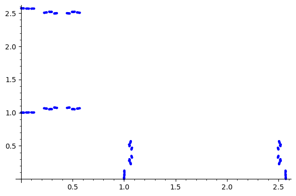
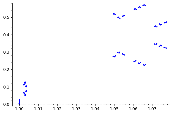
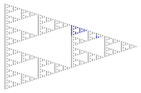
For an illustration of the following result see Figure 13.
Theorem 6.19.
Let . Let be the -adic analytic Jaynes-Cummings model given by (6.1). The following statements hold.
-
(1)
If , then the fiber consists of a single point at .
-
(2)
If , then the fiber has dimension and a singularity at .
-
(3)
If is a rank critical value, then the fiber is the disjoint union of a -dimensional -adic analytic submanifold, maybe empty, and the circle formed by the critical points for that value:
-
(4)
For the rest of values of , the fiber is a -dimensional -adic analytic submanifold.
Proof.
The same as Theorem 6.11. The changes are:
-
•
If the number is never a square. This happens because ends in and has order multiple of , so ends in and also has order multiple of . No number with this form, after subtracting , ends in (the ending stays as if its order is negative, changes to if it is zero, or changes to if it is positive).
-
•
No point other than can have as image. This is because, if it was so,
would be a square, so is also a square. Hence, ends in and has odd order. But should end in , so ends in . There is no number ending in and with odd order that ends in after adding .
∎
In the case of the rank critical values, Figure 13 seems to imply that the fiber only consists of the critical points. We have not been able to deduce this from the formula, and it may well happen that the figure is not taking into consideration enough points to pick one in the fiber.
7. Non-degeneracy and normal forms of the critical points of
In this section we verify the non-degeneracy of the critical points of the -adic Jaynes-Cummings model given by (6.1), and obtain a normal form near each critical point. Because we are dealing with -valued maps, the calculations have to be done, even if they are analogous to the case of -valued maps. Also, in the case the calculations are mathematical folklore among experts and we did not see them explicitly written elsewhere so that we could cite them here (the statement is given in [32, Proposition 2.1, paragraph 3]), and since the example we are presenting here is foundational for the theory of -valued integrable systems, we want to present the calculations explicitly.
Also, it should be noted that Williamson’s full classification [44] is not (yet) available in the -adic case, so all conclusions concerning the example have to be done by hand. (In the real case there are some simplifications as in [44, Section 5]).
The following definition is analogous to the one for the real case, [28, Definition 3.1]. In [7, 13, 23] there are criteria for deciding whether a point is non-degenerate, for rank and points.
Definition 7.1.
Let be a -adic analytic symplectic four-manifold. Let be an integrable system on and let be a critical point of . If , the is called non-degenerate if the Hessians span a Cartan subalgebra of the symplectic Lie algebra of quadratic forms on the tangent space . If one can assume that . Let be an embedded local -dimensional symplectic submanifold through such that and is transversal to the Hamiltonian vector field defined by the function . The critical point of is called (transversally) non-degenerate if is a non-degenerate symmetric bilinear form on .
First we treat the case of rank points.
Proposition 7.2.
Let be a prime number. The critical points in the preimage under the Jaynes-Cummings model given by (6.1) of the curves:
are non-degenerate of rank , and of “elliptic-regular” type: for a point , where with , consider the map
given by
where
The map is a linear symplectomorphism, i.e. an automorphism such that , where
and is the Jaynes-Cummings symplectic linear form at . In addition, satisfies the equation
where
and with
In particular, if is given by
then
Proof.
The point is of rank by Theorem 6.2. First, we want to be quadratic near . This means that . Let .
which is true for proportional to . We will take for the moment this combination, and the proportionality constant will be determined later.
In the coordinates we have:
The combination
gives
Choosing the basis given by the columns of and changing, becomes
Let be the coordinates after this change. Note that does not appear in , which is expected because
and both Hessians of and should vanish at , which is proportional to .
Now we have that
so the linear term in is , and
and
We want to remove the terms in and in these expressions. In order to do this, we first change the coordinates and :
The result is that
which is almost the expression we want. Now we change and :
This does not affect , because they do not use , so taking the matrix as above, we have the desired result for .
Making the changes in ,
and we are done. ∎
The following result is a direct consequence of the proof of Proposition 7.2, which can be simplified in the case of the real Jaynes-Cummings model.
Corollary 7.3.
In the case of the real Jaynes-Cummings model given in Proposition 1.1, we have that:
| (7.1) |
where with
and are local coordinates around such that
In particular, if
then
Proof.
If we apply the proof of Proposition 7.2 word by word, we end up with the expressions
and
where the constants depend on . At the critical points must be sum of two squares, which in the real case means . (The endpoints of this interval correspond to a rank point.) This implies that for all . Now we can make further simplifications:
-
(1)
Multiply the coordinates and by , so that
and
-
(2)
Multiply by and divide by the same amount. This does not alter and makes
-
(3)
Multiply by (in what follows we call this factor ). After this step,
and
-
(4)
Multiply by , so that takes its final form and is not altered.
-
(5)
Multiply the first row of by and the second by . The simplification is complete.
∎
Remark 7.4.
In the -adic case the simplifications in the proof of Corollary 7.3 are in general not possible: we need to take roots of the constants , which is only possible for some values of and .
Remark 7.5.
We do not know how/if some form of Eliasson and Vey’s Theorem [15, 16, 36, 41, 42] holds in the -adic case (the analytic case of this theorem is due to Rüßmann [36] for two degrees of freedom and Vey [41] in arbitrary dimension). In the real case Eliasson’s Theorem (assuming that there are no hyperbolic components) says that there is a local diffeomorphism and symplectic coordinates such that , where is one of the elliptic, real or focus-focus models. In the real-elliptic case, if we derive this expression twice we obtain the linear statement we have proved, in the simplified form (7.1). The term is not in the elliptic model , but it appears when deriving (it comes from a second derivative of ).
Now the rank points. We know that there are two: (whose image is ) and (whose image is ). Both have a singularity, however, the two singularities have different types.
Proposition 7.6.
Let be a prime number. Let be the -adic Jaynes-Cummings model given by (6.1). The point is non-degenerate of rank , and of “elliptic-elliptic” type: consider the map
given by
The map is a linear symplectomorphism, i.e. an automorphism such that , where
and is the Jaynes-Cummings symplectic linear form at . In addition, satisfies the equation
where with
Proof.
The point has rank because . The Hessians are
To see that the point is non-degenerate, we take a linear combination of these matrices and multiply it by :
The characteristic polynomial of this matrix is
that has, in general, four different roots (in if , or in a degree extension otherwise). Hence, the point is non-degenerate.
To show the local expression for , we have that
and
where
In the basis formed by the columns of , the Hessians of and have the forms of the matrices and , which gives the formula we want. We also have that
hence in the new coordinates is . ∎
Remark 7.7.
Identifying a Hessian with its quadratic form, the result in Proposition 7.6 can be written
In the real case the can be eliminated from the expression of for the rank points in a similar way to Corollary 7.3: first divide all coordinates by and then adjust to recover the form of . In the -adic case, this can be done only if is a square modulo (that is, if ).
Proposition 7.8.
Let be a prime number. Let be the -adic Jaynes-Cummings model given by (6.1). The point is non-degenerate of rank , and of “focus-focus” type: consider the map
given by
The map is a linear symplectomorphism, i.e. an automorphism such that , where
and is the Jaynes-Cummings symplectic linear form at . In addition, satisfies the equation
where with
Proof.
Again, the rank is because at this point . Now the Hessians are
Taking a linear combination and multiplying by the inverse of the matrix of the symplectic form,
The characteristic polynomial is now
that has again four different roots (maybe not in , but in a degree extension). Hence, the point is non-degenerate. It is only left to find the matrix which makes the following equalities hold:
and
The matrix we are looking for is
and we can see that in the new basis becomes . ∎
Appendix A Basic -adic theory
In this appendix we review the basic -adic theory we need in the main part of the paper and derive some results (such as Proposition A.9), the statements of which we did not find explicitly written elsewhere and which we need in the main part of the paper.
A.1. Properties of the -adic numbers
The field of real numbers is defined as a completion of with respect to the normal absolute value on . Analogously, the field of -adic numbers can be defined as a completion of with respect to a non-archimedean absolute value. Throughout this section we fix a prime number .
Following [18, Definitions 2.1.2 and 2.1.4], the -adic valuation on is the function
defined as follows: for each integer , , let be the unique positive integer satisfying
We extend to the field of rational numbers as follows: if , then
Also, for any , we define the -adic absolute value of by
if , and we set .
One can check that is a non-archimedean absolute value:
-
•
for all ,
-
•
for all ,
-
•
for all .
Theorem A.1 ([18, Theorem 3.2.13]).
There exists a field with a non-archimedean absolute value , such that the following statements hold.
-
(1)
There exists an inclusion , and the absolute value induced by on via this inclusion is the -adic absolute value.
-
(2)
The image of under this inclusion is dense in with respect to the absolute value .
-
(3)
is complete with respect to the absolute value .
The field satisfying (1), (2) and (3) is unique up to isomorphism of fields preserving the absolute values.
Following [18, Definition 3.3.3], the ring of -adic integers is defined by:
Proposition A.2 ([18, Proposition 3.3.4]).
For any , there exists a Cauchy sequence converging to , of the following type:
-
•
satisfies ;
-
•
for every we have .
The sequence with these properties is unique.
Proposition A.2 implies that any -adic number can be written uniquely as where and , which is called -adic expansion of . We have that the absolute value defined in Theorem A.1, , coincides with . This motivates to define and call it order of .
In the following we will drop the subindex in and .
The topology of the -adic field is very different from the reals, despite both being completions of the rationals with different metrics.
Theorem A.3 ([18, Corollaries 3.3.6 and 3.3.7]).
The following statements hold.
-
•
The -adic metric on given by satisfies the inequality This makes an ultrametric space.
-
•
is totally disconnected, that is, all sets with more than one element are disconnected.
-
•
The balls in the ultrametric space are given by
Replacing by any other point in the ball does not change the ball.
-
•
All balls are compact and open (in particular, is compact and open). is locally compact.
Corollary A.4.
An open subset of is a disjoint union of balls.
Proof.
This is a consequence of the previous theorem and [38, Lemma 1.4]. ∎
The following is an important theorem in -adic algebra. For a polynomial , we denote by the formal derivative of .
Theorem A.5 (Hensel’s lifting, [18, Theorem 3.4.1 and Problem 112]).
Let be a polynomial in . Let be a -adic integer, and . If , there exists such that and .
Corollary A.6.
If and , if and only if and , or and .
Proof.
The implication to the left is obvious if . If , we have that for some , so
To prove the other implication, we apply Hensel’s lifting to and . If , we have and , so there is with and . This implies , so , as we wanted. The case is similar but with . ∎
The following result is a consequence of the absolute value being non-archimedean.
Proposition A.7 ([18, Corollary 4.1.2]).
A series in converges if and only if the sequence of its terms converges to zero.
Now we define some concepts we need concerning the topology of .
-
•
For any , we define the -adic norm on by
-
•
The balls in are defined with this norm:
The resulting topology in is the -th product of the topology in .
-
•
For any , the limit of a function , where is an open set in , at a point , is equal to if and only if, for any , there is such that ; we denote this by .
-
•
is continuous at if .
-
•
is continuous at if it is continuous in each (this is equivalent to the standard definition of continuous function between two topological spaces).
Because of Theorem A.3, continuous functions look very different from their real counterparts. For example, the functions and are both continuous in , despite having discrete images.
-adic differentiation is defined in analogy to the real case. Let be an open set. (Actually, by Corollary A.4, we can take to be a ball.) A function is differentiable at if there is a linear map such that
It is easy to check that If is differentiable at , then the limit
exists and The derivatives of elementary functions give the same result in the real and -adic cases. For example, and The easiest way of seeing this is just taking the limits:
The previous results convey, at a formal level that there is a high degree of similarity between the real and -adic cases. However, upon closer analysis, one realizes that this is not necessarily the case. Indeed, consider the function given by where is the -adic expansion of . We can check that which implies that the function is continuous, and also that the function has zero derivative everywhere. In the real case, such a function would necessarily be constant. However, is not only non-constant, but it is actually injective.
A.2. -adic initial value problems
It is not a good idea, at least in principle, to use differentiable functions in general in the context of -adic symplectic geometry: for any differential equation, the solution will not be unique, not even locally, because we could add an injective function with zero derivative to the solution and we will have another solution. The workaround is to restrict to analytic functions.
A power series in is given by where means and are coefficients in . The following result is well-known and will be useful to us later.
Proposition A.8 ([18, Proposition 4.2.1]).
Consider a power series in one variable in . The convergence radius of the series is given by
Then:
-
•
If (that is, ), then converges only when .
-
•
If (that is, ), then converges for every .
-
•
If and (that is, ), then converges if and only if (that is, ).
-
•
If and does not tend to zero, then converges if and only if (that is, ).
Let be an open set. A function is analytic [38, page 38] if can be expressed as where , for some and , and there is a power series converging in such that for every .
Proposition A.9 (-adic analytic initial value problem).
Let be open subsets of . An initial value problem, of the form
where is analytic, and , has an analytic solution in a neighborhood of . The solution is locally unique among analytic functions, that is, any other solution coincides with it near .
Proof.
We may assume without loss of generality (shrinking if necessary) that is given by a power series in , centered at . Take The initial value implies that . The differential equations give
The degree part at the left-hand side gives and the right-hand side gives a polynomial in . Hence is uniquely determined from the previous ones. The resulting is a solution in a neighborhood of the origin (the intersection of with the convergence domain of the series), and it is locally unique because any other analytic solution would have the same power series around and so it coincides with near this point. ∎
Remark A.10.
Proposition A.9 implies that we can now speak of “the solution” of an analytic differential equation, maybe not in the sense of “the unique solution”, but in the sense of “the germ of every solution”.
A.3. Properties of trigonometric and exponential series on the -adic field
In the -adic setting, one defines the following analogs of the well known sine, cosine, and exponential series in the real case.
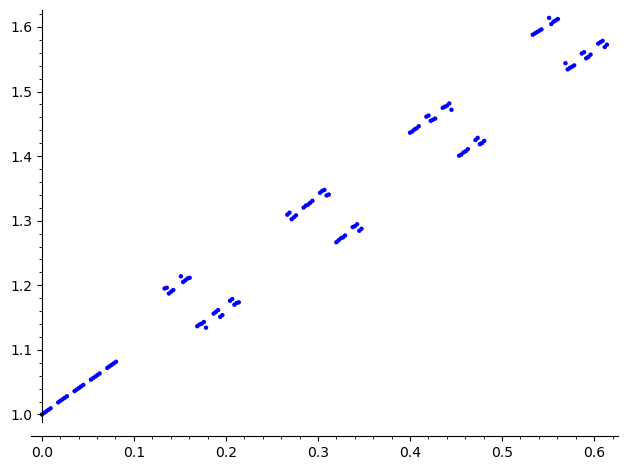
These expressions, when adequately restricted, define functions which have the following properties (quite different, again, from the real counterparts), which we have not found as explicitly written elsewhere but that for us were essential in Section 4.1, so we prove all of them.
A study of the -adic exponential series may be found in Conrad [8, Section 4]. The first statement below corresponds to [8, page 13 and Examples 4.2 and 8.15]. The sine series in the second statement below is mentioned in [8, page 21] where the author also indicates that the proof that the exponential series converges on for and on for also applies to the case of the p-adic sine series; this corresponds to the first part of the second statement below. We have not found the second part of the second statement below or the third statement below explicitly written here or elsewhere. We do not have a complete explicit description of the image of the cosine series, and hence the claim for this part (third part of statement) refers to an inclusion into a set, not an equality. The proof method we follow below to determine the domain and image of the exponential series is essentially self-contained and the calculations are carried out in a slightly different form (but using essentially the same technique) than how they are presented in [8].
Proposition A.11.
Let if , otherwise .
-
(1)
The domain of the exponential series is . Its image is .
-
(2)
The domain of the sine series is . Its image is .
-
(3)
The domain of the cosine series is . Its image is contained in .
Proof.
In order to determine the domains of definition of these functions, it suffices to apply Proposition A.8. We prove the claim for the exponential and the other two cases are analogous:
Let , so that the sum in actually ends in .
So we have . For , this implies that the convergence domain of the series is . For , we have , and This equals for an that is a power of , so it does not tend to infinity, and the domain is .
Now we turn to the image. Let be the -adic expansion for , and the same for . If , we have that and the series implies that . Now
| (A.1) |
Taking modulo at both sides, the only term with in the right corresponds to , and it is an empty product that equals , and the rest of terms have , which makes them multiples of . So we have . If , we take modulo . The only terms left on the left-hand side are . On the right all terms with have automatically and , so they are multiples of and the right-hand side is still . This implies . In any case, we have proved that the image is contained in .
Conversely, suppose that . Then the construction of with can be done inductively on . Supposing that we already have for , we will deduce . In order to do this, we take mod on both sides of (A.1) and get in this way that By induction hypothesis, the components with on the left coincide modulo with those on the right, so the expression simplifies to
for some . One term in the right-hand side is exactly , and the rest only depend on for , which we already know. This means that we can obtain a unique value for , and the induction step is complete.
The case of the sine series is similar to the exponential, but with , because there is no term of degree in the sine series.
For the cosine series, we start in the same way, noticing that
For , we take modulo , and obtain again , as we want. For , we take modulo . At the right, all terms with have and This means only survives from this sum, and , as we wanted. ∎
Appendix B -adic analytic functions, vector fields and forms
Throughout this section is a fixed prime number. The content of this section is directly analogous to the real case, we include it here for completeness and also because it gives us the chance to discuss some peculiarities of the -adic case which do not appear in the real case.
Given a -adic analytic manifold , a function is (-adic) analytic [38, page 49] if it is analytic as a map between manifolds, that is, for the charts of , is analytic on . Let be the space of analytic maps .
A tangent vector to is a linear map such that for all . Let be the space of tangent vectors to . If is a -adic analytic manifold, then has also the structure of an analytic manifold. An analytic vector field on is an analytic map that assigns a tangent vector to each point, or equivalently, a linear map such that for all . Let be the space of vector fields in . An analytic -form in is a linear antisymmetric map Let be the space of -forms in .
The pullback of by and the push-forward of a vector are defined exactly as in the real case. Similarly, if is bi-analytic, the push-forward of a vector field is defined as in the real case and denoted by . Similarly for the pullback of a form , denoted as usual by .
In the linear case where is an open subset of , as is paracompact, analytic functions can be given by a family of power series, each one converging in an element of a partition of in open sets (actually, balls):
for any and some coefficients . This allows us to define the vector field , for open in is given by
for , where and is defined as . It follows that for any function and , there are functions such that
| (B.1) |
and . Also, for any and , we have that . This says that the vector fields form a basis of the space , or locally, that the vectors form a basis of the vector space .
In the real case, the proof of the formula (B.1) is usually done by a method involving integrals (as for example in [17, Theorem 3.4]). One has to be careful if one wants to derive it for -adic smooth functions (which we have not defined, since we are restricting to the analytic case, but the definition is the natural one) because it is more delicate to work with integrals. However, the formula can still be derived without integrals, by using induction on . Supposing it is true for , to prove it for we only need to find such that
The formula already gives the value of for . For we take to be the partial derivative of with respect to in those points. By smoothness of , this function is also continuous on those points, and in fact smooth.
Finally, if and , the differential form is defined as the map sending a vector field to . In particular, if
we have . Hence, the -forms are a basis of , dual to the basis of .
All of the previous definitions generalize to the context of -adic analytic manifolds. Indeed, let be a -adic analytic manifold and an open set of . The vector field is defined as the push-forward by of the corresponding vector field in , and the -forms are defined as the pullback of the corresponding forms in . (With this definition, the vector fields and the -forms are again bases of their respective spaces.)
The wedge operation is defined as usual, and similarly for the differential operator
extending linearly to all forms, where is shorthand for . A form is closed if its differential is . Also, given a -form and a vector field , is defined as usual.
Appendix C -adic hamiltonian actions
In Sections 4 and 5 of the paper we discuss Hamiltonian -actions, which are essential to understand the Jaynes-Cummings model. In this appendix we briefly recall the concept of -adic Hamiltonian action.
Definition C.1.
A -adic analytic Lie group is a group endowed with a structure of -adic analytic manifold that makes the group operations analytic. The Lie algebra associated to a group is given, as usual, by the left-invariant vector fields, identified by tangent vectors at the identity.
The first example is , whose Lie algebra is itself with the Lie bracket equal to . Unlike real Lie groups, we can restrict this: is still a group, and it contains all the elements near the identity of , hence it has the same Lie algebra, and the same applies to . (Note that the Lie algebra still characterizes locally the group.)
It is a known result about -adic Lie groups that every -adic Lie group is paracompact [38, Corollary 18.8]. Hence (Theorem 3.1) it is an ultrametric space.
In what follows let be a -adic Lie group with Lie algebra and a -adic symplectic manifold. We have the canonical actions of in itself:
By slight abuse of notation, we call (as usual when speaking of Lie algebras)
for and . (These two are tangent vectors at .)
Definition C.2.
Let be a -adic analytic Lie group with Lie algebra and a -adic analytic symplectic manifold. A -action is analytic if it is analytic as a map between the manifolds and . Given such an action, for , we denote by the map from to sending to . The action is symplectic if, for any , is a symplectomorphism.
Given a symplectic action of over , and a vector , we define a vector field assigning to each point the push-forward of by the application , that is,
for .
Definition C.3.
Let be a -adic analytic Lie group with Lie algebra and a -adic analytic symplectic manifold. We say that the action is weakly Hamiltonian if, for any , the induced vector field is Hamiltonian with Hamiltonian function . The momentum map of a weakly Hamiltonian action is the map defined by for all . The action is called Hamiltonian if, for all and ,
(Note that if is a tangent vector at the identity, is a tangent vector at and is again a tangent vector at the identity.)
Remark C.4.
In terms of momentum map, the condition for the action to be Hamiltonian is written as . In the well studied case of being a compact connected Abelian Lie group (a torus) acting on a (real) symplectic manifold, a weakly Hamiltonian action is Hamiltonian if and only if is -invariant. If this torus acts on a compact , which is the setting of the well known convexity theorem of Atiyah [2] and Guillemin-Sternberg [19], then being weakly Hamiltonian is equivalent to being Hamiltonian.
References
- [1] J. Alonso, H. R. Dullin, S. Hohloch: Taylor series and twisting-index invariants of coupled spin-oscillators, Journal of Geometry and Physics 140 (2019) 131-151.
- [2] M. Atiyah: Convexity and commuting Hamiltonians, Bull. Lond. Math. Soc. 14 (1982), 1–15.
- [3] S. Awodey, Á. Pelayo, M. A. Warren: Voevodsky’s univalence axiom in homotopy type theory. Notices Amer. Math. Soc. 60(9) (2013), 1164–1167.
- [4] O. Babelon, L. Cantini, B. Douçot: A semi-classical study of the Jaynes-Cummings model, J. Stat. Mech. Theory Exp. (2009), no. 7, P07011, 45 pp.
- [5] O. Babelon, B. Douçot: Classical Bethe Ansatz and normal forms in an integrable version of the Dicke model, Phys. D 241 (2012) 2095–2108.
- [6] O. Babelon, B. Douçot: Higher index focus-focus singularities in the Jaynes-Cummings-Gaudin model: symplectic invariants and monodromy, J. Geom. Phys. 87 (2015), 3–29.
- [7] A. V. Bolsinov, A. T. Fomenko: Integrable Hamiltonian Systems: Geometry, Topology, Classification, CRC Press, 2004.
- [8] K. Conrad: Infinite series in p-adic fields. Available in section of Expository papers (algebraic number theory) of http://www.math.uconn.edu/~kconrad.
- [9] G. S. Djordjevic, B. Dragovich: p-adic and adelic harmonic oscillator with time-dependent frequency. Theor. Math. Phys. 124 (2000), 1059–1067.
- [10] B. Dragovich: p-Adic and Adelic Quantum Mechanics. Proceedings of the First Int. Conf. on p-Adic Mathematical Physics, 1-5 October 2003, Moscow.
- [11] B. Dragovich: Adelic harmonic oscillator. International Journal of Modern Physics A 10(16) (1995): 2349–2365.
- [12] B. Dragovich, A. Yu. Khrennikov, S. V. Kozyrev, I. V. Volovich: On p-adic mathematical physics. P-Adic Numbers, Ultrametric Analysis, and Applications 1 (2009), 1–17.
- [13] H. R. Dullin, Á. Pelayo: Generating hyperbolic singularities in semitoric systems via Hopf bifurcations. J. Nonlinear Sci. 26 (2016), 787–811.
- [14] Y. Eliashberg: Recent advances in symplectic flexibility. Bull. Amer. Math. Soc. 52(1) (2015), 1–26.
- [15] L. H. Eliasson: Normal forms for hamiltonian systems with Poisson commuting integrals – elliptic case. Comment. Math. Helv. 65 (1990) 4–35.
- [16] L. H. Eliasson: Hamiltonian Systems with Poisson Commuting Integrals, PhD thesis, University of Stockholm, 1984.
- [17] J. M. Gamboa, J. M. Ruiz: Iniciación al Estudio de las Variedades Diferenciables, Sanz y Torres, 2020.
- [18] F. Q. Gouvea: -adic Numbers, Springer-Verlag 1993.
- [19] V. Guillemin, S. Sternberg: Convexity properties of the moment mapping. Invent. Math. 67 (1982), 491–513.
- [20] R. Gutiérrez-Jáuregui, G. S. Agarwal: Probing the spectrum of the Jaynes-Cummings-Rabi model by its isomorphism to an atom inside a parametric amplifier cavity, Phys. Rev. A 103 (2021) Paper No. 023714, 9 pp.
- [21] E. T. Jaynes, F. W. Cummings: Comparison of quantum and semiclassical radiation theories with application to the beam maser. Proc. IEEE 51(1) (1963), 89–109.
- [22] N. Koblitz: -adic Numbers, -adic Analysis, and Zeta-Functions. Springer, 1984.
- [23] Y. Le Floch, Á. Pelayo: Symplectic geometry and spectral properties of classical and quantum coupled angular momenta. J. Nonlinear Sci. 29 (2016), 655–708.
- [24] Y. Le Floch, Á. Pelayo, S. Vũ Ngọc: Inverse spectral theory for semiclassical Jaynes-Cummings systems, Math. Ann. 364 (2016) 1393-1413.
- [25] J. Palmer, Á. Pelayo, X. Tang: Semitoric systems of non-simple type. Preprint, arxiv:1909.03501.
- [26] Á. Pelayo: Hamiltonian and symplectic symmetries: an introduction. Bull. Amer. Math. Soc. 54(3) (2017), 383–436.
- [27] Á. Pelayo: Symplectic and inverse spectral geometry of integrable systems: a glimpse and open problems. Top. Appl. 339 Part A (2023) 108577.
- [28] Á. Pelayo, T. Ratiu, S. Vũ Ngọc: Fiber connectivity and bifurcation diagrams of almost toric integrable systems. Journal of Symplectic Geometry 13(2) (2015), 343–386.
- [29] Á. Pelayo, V. Voevodsky, M. A. Warren: A univalent formalization of the -adic numbers. Math. Struct. in Comp. Science 25 (2015), 1147–1171.
- [30] Á. Pelayo, S. Vũ Ngọc: Semitoric integrable systems on symplectic -manifolds. Invent. Math. 177 (2009), 571–597.
- [31] Á. Pelayo, S. Vũ Ngọc: Constructing integrable systems of semitoric type. Acta Math. 206 (2011), 93–125.
- [32] Á. Pelayo, S. Vũ Ngọc: Hamiltonian dynamics and spectral theory for spin-oscillators. Comm. Math. Phys. 309 (2012) 123–154.
- [33] Á. Pelayo, M. A. Warren: Homotopy type theory. Gazette des Mathématiciens Société Mathématique de France 42 (2014), 95–110.
- [34] Á. Pelayo, M. A. Warren: Homotopy type theory and Voevodsky’s univalent foundations. Bull. Amer. Math. Soc. 51 (2014), 597–648.
- [35] J. M. Raimond, M. Brune, S. Haroche: Colloquium: Manipulating quantum entanglement with atoms and photons in a cavity, Rev. Modern Phys. 73 (2001) 565–582.
- [36] H. Rüssmann: Über das Verhalten analytischer Hamiltonscher Differentialgleichungen in der Nähe einer Gleichgewichtlösung. Math. Ann., 154 (1964), 285–300.
- [37] F. Schlenk: Symplectic embedding problems: old and new. Bull. Amer. Math. Soc. 55(2) (2018), 139–182.
- [38] P. Schneider: -adic Lie Groups, Springer-Verlag 2011.
- [39] B. W. Shore, P. L. Knight: The Jaynes-Cummings model, J. Modern Opt. 40 (1993) 1195–1238.
- [40] J. P. Serre: Classification des varietes analytiques -adiques compactes. Topology 3 (1965) 409–412.
- [41] J. Vey: Sur certains systèmes dynamiques séparables. Amer. J. Math., 100 (1978), 591–614.
- [42] S. Vũ Ngọc, C. Wacheux: Smooth normal forms for integrable hamiltonian systems near a focus-focus singularity. hal preprint oai:hal.archives-ouvertes.fr: hal-00577205, arXiv: 1103.3282.
- [43] A. Weinstein: Symplectic geometry, Bull. Amer. Math. Soc. 5(1) (1981), 1–13.
- [44] J. Williamson: On the algebraic problem concerning the normal forms of linear dynamical systems. American Journal of Mathematics 58(1) (1936), 141–163.