BiTrack: Bidirectional Offline 3D Multi-Object Tracking Using Camera-LiDAR Data

Abstract

Compared with real-time multi-object tracking (MOT), offline multi-object tracking (OMOT) has the advantages to perform 2D-3D detection fusion, erroneous link correction, and full track optimization but has to deal with the challenges from bounding box misalignment and track evaluation, editing, and refinement. This paper proposes “BiTrack”, a 3D OMOT framework that includes modules of 2D-3D detection fusion, initial trajectory generation, and bidirectional trajectory re-optimization to achieve optimal tracking results from camera-LiDAR data. The novelty of this paper includes threefold: (1) development of a point-level object registration technique that employs a density-based similarity metric to achieve accurate fusion of 2D-3D detection results; (2) development of a set of data association and track management skills that utilizes a vertex-based similarity metric as well as false alarm rejection and track recovery mechanisms to generate reliable bidirectional object trajectories; (3) development of a trajectory re-optimization scheme that re-organizes track fragments of different fidelities in a greedy fashion, as well as refines each trajectory with completion and smoothing techniques. The experiment results on the KITTI dataset demonstrate that BiTrack achieves the state-of-the-art performance for 3D OMOT tasks in terms of accuracy and efficiency.

I Introduction

Many applications require offline multi-object tracking (OMOT) technologies to achieve object trajectories of high accuracy, such as movement analysis and dataset annotation. Real-time multi-object tracking (MOT) usually uses either tracking-by-detection[1, 2, 3, 4] or joint detection and tracking[5] schemes. In contrast, OMOT prefers the former because many post-processing and global optimization techniques rely on detection results. Most OMOT association frameworks can fall into two categories: (1) optimization and clustering of detection results[6, 7, 8], and (2) editing and refinement of initial trajectories[9, 10, 11, 3, 4]. Both categories rely on the quality of detection. Due to the lack of sequential information, the former likely suffers from context inconsistency and computational instability; as based on sequential tracking results, the latter usually yields guaranteed performance. Many methods utilize 2D detection results to improve 3D detection, where the performance is limited by either the cascade pipeline[12] or various 2D-3D object registration errors[13]. Therefore, to develop a post-processing based OMOT framework (as shown in Fig. 1), the following technical challenges have to be well dealt with:

1. 2D-3D object registration. Sensor miscalibration, inter-object occlusion, detection inaccuracy, and bounding box misalignment cause many object registration noises for 2D-3D object post-fusion.

2. Initial trajectory generation. The association accuracy relies on the quality of object similarity metrics and track management mechanisms, which suffer from complex object movements, detection false alarms, and object re-appearances.

3. Trajectory post-processing. Trajectory post-processing includes two aspects: (1) the re-organization of multiple trajectories and (2) the refinement of each single trajectory. The former requires track quality evaluation and association techniques, while the later demands trajectory completion and regression skills. Both aspects suffer from object temporal contradictions, tracking uncertainties, and heavy computations.

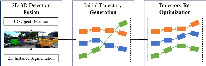
Figure 1: A post-processing based offline 3D multi-object tracking framework with three main stages.

TABLE I: A methodological comparison between BiTrack and typical 2D-3D object detection and tracking methods

[c] Category 2D-3D Object Fusion Initial Trajectory Generation Trajectory Post-Processing Similarity Evaluation Track Management Multi-Trajectory Fusion Single-Trajectory Refinement CLOCs[13] 3D Object Detection Box-Level Object Fusion - - - - AB3DMOT[2] 3D MOT $\times$ 3D IoU / 3D Center Distance Online Hit-Miss $\times$ $\times$ JRMOT[12] 3D MOT Frustum-Based Detection Pipeline Appearance / 2D IoU / 3D IoU Online Hit-Miss $\times$ $\times$ AHC_ETE[8] 2D OMOT $\times$ Appearance / 2D Center Distance $\times$ Hierarchical Clustering $\times$ TMOH[10] 2D OMOT $\times$ Appearance Occlusion-Aware Online Miss Bidirectional Trajectory Replacement $\times$ ReMOT[9] 2D OMOT $\times$ Appearance / 2D Center Distance Online Hit-Miss Forward Tracklet Split-Merge $\times$ StrongSORT[4] 2D OMOT $\times$ Appearance & 2D Center Distance Online Hit-Miss Tracklet Association LI & GPR 3DAL[11] 3D OMOT $\times$ 3D IoU / 3D Center Distance Online Hit-Miss $\times$ Deep Learning Regression PC3T[3] 3D OMOT $\times$ 3D Center Distance Online Miss $\times$ Kalman Filter Prediction BiTrack (ours) 3D OMOT Point-Level Object Fusion 3D Normalized Center Distance Improved Offline Hit-Miss Bidirectional Trajectory Split-Merge LI & CSA & GPR

• “$\times$”: unsupported functionality, “LI”: linear interpolation, “CSA”: confidence-based size averaging, “GPR”: Gaussian process regression

A number of detection fusion methods[13] use the 2D intersection-over-unions (IoUs) between 2D bounding boxes and the perspective views (PVs) of 3D bounding boxes as fusion cues, which may lead to ambiguities due to occlusions. Most real-time MOT methods[1, 2, 12, 4] employ bounding box-based metrics for object similarities as well as life cycle-based mechanisms for the track management, while few of them consider metric limitations or the nature of detection errors. Many OMOT methods perform trajectory refinement with clustering[8], association[4], or regression[11, 4] techniques but they can hardly re-organize the existing trajectories with global sequential information.

This paper presents “BiTrack”, an OMOT framework which enables robust 2D-3D detection fusion, reliable initial trajectory generation, and efficient trajectory re-optimization. The contributions of this work include:

1. Development of a 2D-3D detection fusion module that utilizes point-level representations and object point densities to achieve robust object registration.

2. Development of a trajectory generation module that employs a scale-balanced object similarity metric and an offline-oriented track management mechanism to achieve reliable 3D MOT.

3. Development of a trajectory re-optimization module that utilizes a priority-based fragment optimization as well as trajectory completion and smoothing skills to achieve efficient bidirectional trajectory fusion and single-trajectory refinement.

4. Release of the source code of this work at https://github.com/Kemo-Huang/BiTrack.

The organization of this paper is as follows. Section II introduces the related detection and MOT methods. Section III states the system setup and the problems to solve. Section IV describes the proposed methods. Section V presents the experiments and analyses. Section VI concludes this paper.

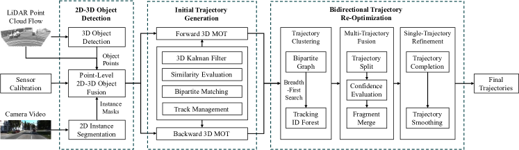
Figure 2: The system architecture of BiTrack.

II Related Work

Typical methods for 2D-3D object detection, real-time MOT and OMOT are summarized in TABLE I. There are many multi-modal detection fusion methods in 3D object detection[14, 13] and 3D MOT[12]. JRMOT[12] adopts the frustum-based fusion method[14] for cascade 2D-3D detection, where the 2D detection stage becomes the bottleneck. CLOCs[13] uses separate detection branches and re-evaluates 3D detection confidences using 2D results. However, the 2D-3D object correspondences are based on 2D IoU, which may suffer from object occlusions.

IoU and the center distance are two prevalent object motion similarity metrics for 2D and 3D MOT[2, 12, 8, 11, 9, 3, 4]. Both metrics provide incomplete spatial information, while 2D appearance similarities are hard to be combined with the latter due to the scale gap[4]. In addition, hit-miss schemes are commonly used in the track management[2, 12, 11, 9, 3, 4] but most of them are only designed for online applications.

Many OMOT methods[10, 9, 4, 11, 3] perform trajectory post-processing based on real-time MOT results, which implicitly demand sequential association. Some methods like min-cost flow[6] and hierarchical clustering[8] can merge detection results from a global graph without sequential cues. However, they usually result in heavy computations and inconsistent object similarities. ReMOT[9] re-evaluates 2D object similarities in a sliding window for tracklet split-merge. TMOH[10] assembles the results from forward and backward data sequences but the object link contradictions are simply handled by replacing the entire trajectory. Furthermore, single-trajectory refinement can be performed in the final stage using physical models[4, 3] or deep learning models[11].

BiTrack follows the refinement scheme for both detection and tracking. In contrast to previous works, this work provides the features of point-level detection fusion, robust motion-based initial trajectory generation, as well as split-merge based bidirectional trajectory re-optimization.

III System Setup and Problem Statement

BiTrack can be divided into three main modules: (1) 2D-3D object detection, (2) initial trajectory generation, and (3) bidirectional trajectory re-optimization, as shown in Fig. 2. The whole pipeline is fully automatic.

Given a sequence of camera and LiDAR inputs, the goal of OMOT is to localize and identify the objects of specific categories in the 3D environment for all frames. For data pre-processing, object detectors localize 2D objects $\boldsymbol{\mathcal{D}}^{\text{2D}}$ and 3D objects $\boldsymbol{\mathcal{D}}^{\text{3D}}$ with detection confidences $\boldsymbol{\mathcal{C}}^{\text{2D}}$ and $\boldsymbol{\mathcal{C}}^{\text{3D}}$ in separate branches. BiTrack performs OMOT as follows.

Firstly, the 2D-3D object fusion module performs the object registration between $\boldsymbol{\mathcal{D}}^{\text{2D}}$ and $\boldsymbol{\mathcal{D}}^{\text{3D}}$ using camera intrinsic parameters $\boldsymbol{K}$, camera-LiDAR extrinsic parameters $[\boldsymbol{R}\mid\boldsymbol{t}]$, and 2D-3D detection similarities $\boldsymbol{\mathcal{W}}^{\text{D}}\in\mathbb{R}^{+}$. The 2D-3D object registration is addressed as a complete bipartite graph matching problem to solve the assignment matrix $\boldsymbol{\mathcal{X}}^{\text{D}}$:

$$\begin{gathered}\boldsymbol{\mathcal{X}}^{\text{D}*}=\mathop{\arg\max}_{X^{\text{D}}}\sum_{D^{\text{2D}}_{i}\in\boldsymbol{\mathcal{D}}^{\text{2D}}}\sum_{D_{j}^{\text{3D}}\in\boldsymbol{\mathcal{D}}^{\text{3D}}}W^{\text{D}}_{i,j}X^{\text{D}}_{i,j}\\ \text{s.t. }\begin{dcases}\sum_{D^{\text{3D}}_{j}\in\boldsymbol{\mathcal{D}}^{\text{3D}}}X^{\text{D}}_{i,j}\leq 1&\forall D^{\text{2D}}_{i}\in\boldsymbol{\mathcal{D}}^{\text{2D}}\\ \sum_{D^{\text{2D}}_{i}\in\boldsymbol{\mathcal{D}}^{\text{2D}}}X^{\text{D}}_{i,j}\leq 1&\forall D^{\text{3D}}_{j}\in\boldsymbol{\mathcal{D}}^{\text{3D}}\\ X^{\text{D}}_{i,j}\in\{0,1\}&\forall D^{\text{2D}}_{i}\in\boldsymbol{\mathcal{D}}^{\text{2D}},\forall D^{\text{3D}}_{j}\in\boldsymbol{\mathcal{D}}^{\text{3D}}\\ \end{dcases}\end{gathered}$$ (1)

The final 3D detection inputs for tracking $\boldsymbol{\mathcal{D}}=\{D^{\text{3D}}_{i}\in\boldsymbol{\mathcal{D}}^{\text{3D}}\mid f^{\text{D}}(D^{\text{3D}}_{i})=1\}$ are selected from $\boldsymbol{\mathcal{D}}^{\text{3D}}$ according to $\boldsymbol{\mathcal{C}}^{\text{3D}}$, $\boldsymbol{\mathcal{W}}^{\text{D}}$, and $\boldsymbol{\mathcal{X}}^{\text{D}*}$ with the detection decision function $f^{\text{D}}(\cdot)$:

$$f^{\text{D}}(D^{\text{3D}}_{i})=\mathds{1}\bigg{[}\left(C^{\text{3D}}_{i}\geq\theta^{\text{det}}\right)\\ \lor\left(\exists D^{\text{2D}}_{j}\in\boldsymbol{\mathcal{D}}^{\text{2D}}:W^{\text{D}}_{i,j}X_{i,j}^{\text{D}*}\geq\alpha\right)\bigg{]}$$ (2)

where $\theta^{\text{det}}$ is the detection confidence threshold, $\alpha$ is the detection similarity threshold, and $\mathds{1}[\cdot]\rightarrow\{0,1\}$ is the indicator function.

Secondly, the initial trajectory generation module performs the association between detected objects $\boldsymbol{\mathcal{D}}$ and predicted objects $\boldsymbol{\mathcal{\hat{D}}}$ with detection-prediction similarities $\boldsymbol{\mathcal{W}}^{\text{T}}\in\mathbb{R}^{+}$. The association is also formulated as the bipartite matching problem to solve the assignment matrix $\boldsymbol{\mathcal{X}}^{\text{T}}$:

$$\begin{gathered}\boldsymbol{\mathcal{X}}^{\text{T}*}=\mathop{\arg\max}_{X^{\text{T}}}\sum_{D_{i}\in\boldsymbol{\mathcal{D}}}\sum_{\hat{D}_{j}\in\boldsymbol{\mathcal{\hat{D}}}}W^{\text{T}}_{i,j}X^{\text{T}}_{i,j}\\ \text{s.t. }\begin{dcases}\sum_{\hat{D}_{j}\in\boldsymbol{\mathcal{\hat{D}}}}X^{\text{T}}_{i,j}\leq 1&\forall D_{i}\in\boldsymbol{\mathcal{D}}\\ \sum_{D_{i}\in\boldsymbol{\mathcal{D}}}X^{\text{T}}_{i,j}\leq 1&\forall\hat{D}_{j}\in\boldsymbol{\mathcal{\hat{D}}}\\ X^{\text{T}}_{i,j}\in\{0,1\}&\forall D_{i}\in\boldsymbol{\mathcal{D}},\forall\hat{D}_{j}\in\boldsymbol{\mathcal{\hat{D}}}\\ \end{dcases}\end{gathered}$$ (3)

Tracked objects $\boldsymbol{\mathcal{D}}^{\prime}=\{D_{i}\in\boldsymbol{\mathcal{D}}\mid g(D_{i})=1\}$ are sequentially selected from $\boldsymbol{\mathcal{D}}$ according to $\boldsymbol{\mathcal{W}}^{\text{T}}$ and $\boldsymbol{\mathcal{X}}^{\text{T}*}$ with the track decision function $f^{\text{T}}(\cdot)$ and the track management function $g(\cdot)$ in case of false alarms and object re-appearances:

$$f^{\text{T}}(D_{i})=\mathds{1}\left[\exists\hat{D}_{j}\in\boldsymbol{\mathcal{\hat{D}}}:W^{\text{T}}_{i,j}X_{i,j}^{\text{T}*}\geq\beta\right]$$ (4)

$$\forall X_{i,j}^{\text{T}*}=1:n^{\text{hit}}(D_{i}) =\begin{cases}n^{\text{hit}}(D_{i})&\text{if }f^{\text{T}}(D_{i})=0\\ n^{\text{hit}}(D_{j})+1&\text{if }f^{\text{T}}(D_{i})=1\end{cases}$$ (5)

$$n^{\text{miss}}(D_{i}) =\begin{cases}n^{\text{miss}}(D_{i})+1&\text{if }f^{\text{T}}(D_{i})=0\\ 0&\text{if }f^{\text{T}}(D_{i})=1\end{cases}$$ (6)

$$g(D_{i})=\begin{cases}1&\text{if }\left(n^{\text{hit}}(D_{i})\geq\theta^{\text{hit}}\right)\land\left(n^{\text{miss}}(D_{i})=0\right)\\ -1&\text{if }n^{\text{miss}}(D_{i})\geq\theta^{\text{miss}}\\ 0&\text{otherwise}\end{cases}$$ (7)

where $\beta$ is the tracking similarity threshold, $n^{\text{hit}},n^{\text{miss}}\in\mathbb{N}_{0}$ are the times of hit and miss, and $\theta^{\text{hit}},\theta^{\text{miss}}\in\mathbb{N}_{0}$ are thresholds. Tracking IDs can only be assigned to confirmed objects $\left(g(\cdot)=1\right)$. Object candidates $\left(g(\cdot)=0\right)$ are used for temporary object prediction while dead objects $\left(g(\cdot)=-1\right)$ are permanently removed. The confirmed objects with the same IDs are connected with object links $\boldsymbol{\mathcal{L}}$ to generate trajectories $\boldsymbol{\mathcal{T}}$. The same detection input $\boldsymbol{\mathcal{D}}$ is used to perform MOT in both forward and backward time directions to generate trajectories $\boldsymbol{\mathcal{T}}^{\text{A}}=\left\{\boldsymbol{\mathcal{D}}^{\text{A}},\boldsymbol{\mathcal{L}}^{\text{A}}\right\}$ and $\boldsymbol{\mathcal{T}}^{\text{B}}=\left\{\boldsymbol{\mathcal{D}}^{\text{B}},\boldsymbol{\mathcal{L}}^{\text{B}}\right\}$.

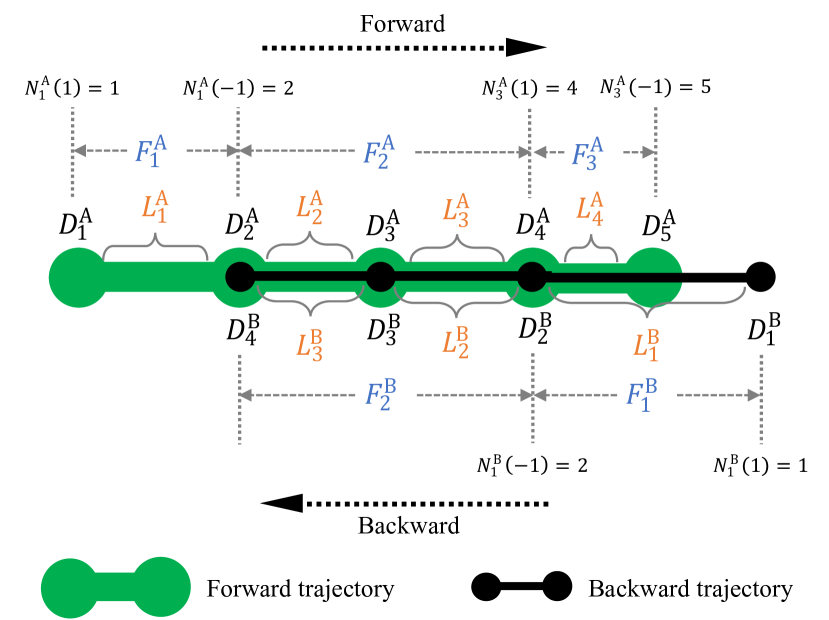
Figure 3: A visual explanation of the symbol definitions for bidirectional trajectory fusion. Best viewed in color.

Finally, the trajectory re-optimization module performs the trajectory fusion and refinement. Fig. 3 demonstrates the symbol definitions. $\boldsymbol{\mathcal{T}}^{\text{A}}$ and $\boldsymbol{\mathcal{T}}^{\text{B}}$ are split into track fragments $\boldsymbol{\mathcal{F}}^{\text{A}}$ and $\boldsymbol{\mathcal{F}}^{\text{B}}$ by the common links $\boldsymbol{\mathcal{L}}^{\text{A}}\cap\boldsymbol{\mathcal{L}}^{\text{B}}$. The fragments are selected via the optimization of fragment priorities under the condition of exclusive object frames:

$$\begin{gathered}\boldsymbol{\mathcal{F}}^{*}=\mathop{\arg\max}_{F}\sum_{F_{i}\in\boldsymbol{\mathcal{F}}^{\text{A}}\cup\boldsymbol{\mathcal{F}}^{\text{B}}}h(F_{i})\\ \text{s.t. }\forall T_{i}\in\boldsymbol{\mathcal{T}},\forall D_{j}\neq D_{k}\in T_{i}:t(D_{j})\neq t(D_{k})\end{gathered}$$ (8)

where $t(\cdot)$ is the frame of an object and $h(\cdot)$ is the fragment priority function:

$$h(F_{i})=\begin{cases}Z&\text{if }F_{i}\in\boldsymbol{\mathcal{F}}^{\text{A}}\cap\boldsymbol{\mathcal{F}}^{\text{B}}\\ \max\left\{N^{\text{A}}_{i}(1),N^{\text{A}}_{i}(-1)\right\}&\text{if }F_{i}\in\boldsymbol{\mathcal{F}}^{\text{A}}-\boldsymbol{\mathcal{F}}^{\text{B}}\\ \max\left\{N^{\text{B}}_{i}(1),N^{\text{B}}_{i}(-1)\right\}&\text{if }F_{i}\in\boldsymbol{\mathcal{F}}^{\text{B}}-\boldsymbol{\mathcal{F}}^{\text{A}}\end{cases}$$ (9)

where $Z\gg N$ is a large integer, $N_{i}(1)$ and $N_{i}(-1)$ stand for the sequential index of the first and last object of $F_{i}$ in the entire trajectory respectively. The fused trajectories $\boldsymbol{\mathcal{T}}^{\text{C}}=\{\boldsymbol{\mathcal{D}}^{\text{C}},\boldsymbol{\mathcal{L}}^{\text{C}}\}$ are obtained from the optimization results $\boldsymbol{\mathcal{F}}^{*}$. The object localization results can be further regressed using the temporal information:

$$\boldsymbol{\mathcal{D}}^{\text{C}}\xrightarrow{\boldsymbol{\mathcal{L}}^{\text{C}}}\boldsymbol{\mathcal{D}}^{+}$$ (10)

The final trajectory outputs become $\boldsymbol{\mathcal{T}}^{+}=\{\boldsymbol{\mathcal{D}}^{+},\boldsymbol{\mathcal{L}}^{\text{C}}\}$.

Therefore, the proposed methods of this work focus on solving the following problems:

1. How to evaluate 2D-3D detection similarities $\boldsymbol{\mathcal{W}}^{\text{D}}$?

2. How to evaluate detection-prediction similarities $\boldsymbol{\mathcal{W}}^{\text{T}}$ and design the hit-miss thresholds $\{\theta^{\text{hit}},\theta^{\text{miss}}\}$?

3. How to perform the optimization of eq. (8) and the refinement of eq. (10)?

IV Proposed Methods

IV-A 2D-3D Object Registration via Points

This work suggests that 2D IoU has three shortages for 2D-3D object fusion: (1) the PVs of 3D bounding boxes are larger than 2D bounding boxes for occluded objects, (2) the PVs of 3D boxes could overlap, and (3) bounding boxes contain space at corners. However, the point density metric between 2D segmentation masks and 3D object points can perfectly tackle those problems.

IV-A1 Point-Level Segmentation

To obtain pixel-level object masks, 2D instance segmentation is required. On the other hand, the 3D bounding boxes obtained from 3D object detection can be directly used to crop LiDAR points for efficiency because 3D objects rarely overlap, especially for rigid bodies. Although cropping LiDAR points within bounding boxes may cost more computations, the operations of multiple data frames can be paralleled by multi-processing for faster execution thanks to the offline setting.

IV-A2 Point-Level Association

After removing background, the correspondence between 2D and 3D objects should be robust against object occlusions. However, sensor miscalibration and detection inaccuracy may still produce registration noises, e.g., a 2D instance mask can include the projected points of multiple 3D objects. Thus, the 2D-3D object similarity should be quantified and the optimization should be performed. This work uses the number of overlapped pixels as $\boldsymbol{\mathcal{W}}^{D}$ and the Hungarian algorithm[15] to solve the equation (1).

Fig. 4 demonstrates the effect of 2D-3D object fusion. The original detection results are generated by the SOTA method VirConv[16] on the KITTI[17] dataset. The proposed 2D-3D fusion method can effectively reduce false alarms, while high-quality detection results can be successfully selected for the trajectory generation stage. The whole fusion procedure is shown in Algorithm 1.

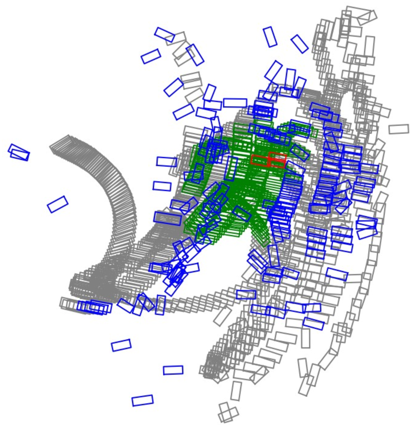
(a) Original detection results[16]

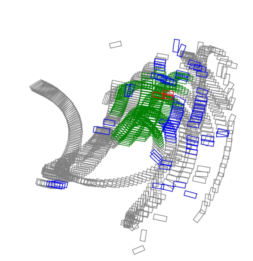
(b) After 2D-3D object fusion

Figure 4: The bird’s-eye view of 2D-3D object fusion results of a sequence. The gray boxes are the objects that the dataset doesn’t care. The green boxes are true positives. The blue boxes are false positives. The red boxes are false negatives. Best viewed in color.

Input: 2D instance masks $\boldsymbol{\mathcal{D}}^{\text{2D}}$;

3D bounding boxes $\boldsymbol{\mathcal{D}}^{\text{3D}}$;

3D detection confidences $\boldsymbol{\mathcal{C}}^{\text{3D}}$;

LiDAR point clouds $\boldsymbol{\mathcal{P}}^{\text{LiDAR}}$;

Sensor calibration parameters $\left\{\boldsymbol{K},[\boldsymbol{R}\mid\boldsymbol{t}]\right\}$;

Output: the selected 3D bounding boxes $\boldsymbol{\mathcal{D}}$;

1 $\boldsymbol{\mathcal{P}}^{\text{3D}}\leftarrow$ Crop the LiDAR points within $\boldsymbol{\mathcal{D}}^{\text{3D}}$ from $\boldsymbol{\mathcal{P}}^{\text{LiDAR}}$;

2 $\boldsymbol{\mathcal{P}}^{\text{2D}}\leftarrow$ Project $\boldsymbol{\mathcal{P}}^{\text{3D}}$ to camera images using $\left\{\boldsymbol{K},[\boldsymbol{R}\mid\boldsymbol{t}]\right\}$;

3 $\boldsymbol{\mathcal{P}}^{\text{2D}}\leftarrow$ Align $\boldsymbol{\mathcal{P}}^{\text{2D}}$ to image pixels;

4 $\boldsymbol{\mathcal{W}}^{\text{D}}\leftarrow\left\{\left|P^{\text{2D}}_{i}\cap D^{\text{2D}}_{j}\right|:P^{\text{2D}}_{i}\in\boldsymbol{\mathcal{P}}^{\text{2D}},D^{\text{2D}}_{j}\in\boldsymbol{\mathcal{D}}^{\text{2D}}\right\}$;

5 $\boldsymbol{\mathcal{X}}^{\text{D}*}\leftarrow$ Solve the eq. (1) using the Hungarian algorithm;

6 $\boldsymbol{\mathcal{D}}\leftarrow\left\{D^{\text{3D}}_{i}\mid f^{\text{D}}(D^{\text{3D}}_{i})=1,D^{\text{3D}}_{i}\in\boldsymbol{\mathcal{D}}^{\text{3D}}\right\}$;

return $\boldsymbol{\mathcal{D}}$

Algorithm 1 Point-level fusion between 2D instance masks and 3D bounding boxes

IV-B Reliable Initial Trajectory Generation

Most 3D MOT methods follow the SORT[1] framework. This work improves the simple 3D MOT baseline[18] with the following techniques for reliable trajectory generation.

IV-B1 Integrated Object Motion similarity Metric

Both 3D IoU and the center distance (CD) metrics have shortages: (1) 3D IoU is too sensitive to object rotation errors, (2) CD does not utilize object size and rotation cues, (3) 3D IoU is incomparable (zero) for separate objects, and (4) the numerical value of CD has no upper bound. To complement these two metrics, this work proposes the normalized center distance (NCD) as the geometric cost. Specifically, the proposed NCD similarity metric $\boldsymbol{\mathcal{W}}^{\text{T}}$ for $D_{i}$ and $\hat{D}_{j}$ is defined as:

$$W^{\text{T}}_{i,j}=1-\frac{d(c_{i},\hat{c}_{j})}{\max\left\{d(v_{i,k},\hat{v}_{j,l})\mid v_{i,k}\in\boldsymbol{\mathcal{V}}_{i},\hat{v}_{j,l}\in\boldsymbol{\mathcal{\hat{V}}}_{j}\right\}}$$ (11)

where $d(\cdot)$ denotes the Euclidean distance, $c$ denotes the center of the bounding box, $\boldsymbol{\mathcal{V}}$ denotes bounding box vertices, $\hat{c}_{j}$ and $\boldsymbol{\mathcal{\hat{V}}}_{j}$ are predicted values from the Kalman filter. The NCD metric provides two main advantages for object similarity evaluation: (1) simultaneous utilization of bounding box positions, sizes, and rotations; (2) normalized numerical value for easy combination with other similarities (e.g., the weighted sum with the cosine similarity between appearance embeddings).

IV-B2 Previous Tracklet Recovery and Double Miss Thresholds

Online tracking results should be reported sequentially but OMOT can break this restriction. Once objects are confirmed, their previous tracklets can be recovered to generate more complete trajectories. Additionally, based on the intuition that false alarms usually do not appear continually, an extra miss threshold is set for track candidates so that false alarms can be quickly rejected.

IV-B3 Velocity Re-initialization

Most SORT-based methods[4, 18, 3] simply initialize object linear velocities as zeros and leave the estimation to the Kalman filter in later updates. However, this inaccurate prior knowledge makes the Kalman filter hard to converge and leads to inaccurate predictions in the early stage. This work proposes to re-initialize the states of objects after they are firstly matched with new measurements. Specifically, the static state is updated exactly as the new measurement and the linear velocity is re-initialized as the translation divided by the passed frames. All state covariances are updated as usual.

IV-C Efficient Trajectory Re-Optimization

Forward and backward trajectory integration realizes false alarms and ID switches, while sequential bounding box refinement realizes false negatives and regression errors. This work proposes three efficient post-processing steps for MOT to improve the link accuracy, the bounding box integrity, and the trajectory smoothness.

IV-C1 Bidirectional Trajectory Clustering

It is necessary to cluster forward and backward trajectories into several groups so that trajectory fusion can be performed within searching boundaries. This work defines the clustering condition as the existence of equal bounding boxes. During the traversal of the bounding boxes, the “two pointers” technique can accelerate the search if bounding boxes are ordered by sequential frames. The trajectories are then formed as a bipartite graph, where the nodes are the trajectory IDs and the edges indicate the existence of equal bounding boxes between two sets of trajectories. The trajectory clustering is basically a breadth-first search (BFS) to transform a bipartite graph into a forest. The whole procedure is shown in Algorithm 2.

Input: Forward tracking IDs $\boldsymbol{\mathcal{A}}$;

Backward tracking IDs $\boldsymbol{\mathcal{B}}$;

Output: Tracking ID clusters $\boldsymbol{\mathcal{S}}$;

1 $\boldsymbol{\mathcal{E}}\leftarrow$ Search the common bounding boxes between forward and backward trajectories via “two-pointers”;

2 $\boldsymbol{\mathcal{G}}\leftarrow$ Build a bipartite graph where $\{\boldsymbol{\mathcal{A}},\boldsymbol{\mathcal{B}}\}$ are nodes and $\boldsymbol{\mathcal{E}}$ are edges;

3 $\boldsymbol{\mathcal{S}}\leftarrow\varnothing$;

4 while $\boldsymbol{(\mathcal{A}}\neq\varnothing)\lor(\boldsymbol{\mathcal{B}}\neq\varnothing)$ do

5       $\boldsymbol{S}^{\text{A}}_{c}\leftarrow\boldsymbol{S}^{\text{B}}_{c}\leftarrow\varnothing$;

6       if $\boldsymbol{\mathcal{A}}\neq\varnothing$ then

7             $A_{i}\leftarrow\text{pop}(\mathcal{A})$;

8             $\boldsymbol{S}^{\text{A}}_{c}\leftarrow\boldsymbol{S}^{\text{A}}_{c}\cup\{A_{i}\}$;

9             $\boldsymbol{\mathcal{M}}\leftarrow\left\{B_{j}\mid\text{edge}(A_{i},B_{j})\in\boldsymbol{\mathcal{E}},B_{j}\in\boldsymbol{\mathcal{B}}\right\}$;

10            

11      else

12             $B_{j}\leftarrow\text{pop}(\mathcal{B})$;

13             $\boldsymbol{S}^{\text{B}}_{c}\leftarrow\boldsymbol{S}^{\text{B}}_{c}\cup\{B_{j}\}$;

14             $\boldsymbol{\mathcal{M}}\leftarrow\left\{A_{i}\mid\text{edge}(A_{i},B_{j})\in\boldsymbol{\mathcal{E}},A_{i}\in\boldsymbol{\mathcal{A}}\right\}$;

15            

16       end if

17      while $|\boldsymbol{\mathcal{M}}|>0$ do

18             $\boldsymbol{\mathcal{N}}\leftarrow\varnothing$;

19             foreach $M_{i}\in\boldsymbol{\mathcal{M}}$ do

20                   if $M_{i}\in\boldsymbol{\mathcal{B}}$ then

21                         $\boldsymbol{\mathcal{N}}\leftarrow\boldsymbol{\mathcal{N}}\cup\{A_{j}\mid\text{edge}(M_{i},A_{j})\in\boldsymbol{\mathcal{E}},A_{j}\in\boldsymbol{\mathcal{A}}\}$;

22                         $\boldsymbol{\mathcal{B}}\leftarrow\boldsymbol{\mathcal{B}}-\{M_{i}\}$;

23                         $\boldsymbol{S}^{\text{B}}_{c}\leftarrow\boldsymbol{S}^{\text{B}}_{c}\cup\{M_{i}\}$;

24                        

25                  else

26                         $\boldsymbol{\mathcal{N}}\leftarrow\boldsymbol{\mathcal{N}}\cup\{B_{j}\mid\text{edge}(M_{i},B_{j})\in\boldsymbol{\mathcal{E}},B_{j}\in\boldsymbol{\mathcal{B}}\}$;

27                         $\boldsymbol{\mathcal{A}}\leftarrow\boldsymbol{\mathcal{A}}-\{M_{i}\}$;

28                         $\boldsymbol{S}^{\text{A}}_{c}\leftarrow\boldsymbol{S}^{\text{A}}_{c}\cup\{M_{i}\}$;

29                        

30                   end if

31                  

32             end foreach

33            $\boldsymbol{\mathcal{M}}\leftarrow\boldsymbol{\mathcal{N}}$;

34            

35       end while

36      $\boldsymbol{\mathcal{S}}\leftarrow\boldsymbol{\mathcal{S}}\cup\left\{\boldsymbol{S}^{\text{A}}_{c}\cup\boldsymbol{S}^{\text{B}}_{c}\right\}$;

37      

38 end while

return $\boldsymbol{\mathcal{S}}$

Algorithm 2 BFS-based trajectory clustering

(a) Forward tracking results

(b) Backward tracking results

(c) Bidirectional fusion results

Figure 5: Visualization of the bidirectional trajectory fusion. Circles represent detected boxes and arrows represent moving directions. Generally, the proposed fusion strategy prefers the object links of tails rather than heads.

IV-C2 Bidirectional Trajectory Fusion

This work suggests that the differences between forward and backward tracking results usually fall into two scenarios: (1) large object velocity changes and (2) incorrect velocity initialization. Hence, the proposed strategy of the bidirectional trajectory fusion is twofold: (1) merges trajectory fragments as many as possible and (2) selects fragments from long trajectories as many as possible. For the clusters whose trajectories have no time contradiction, trajectories are directly merged. For the other clusters, trajectories are split, selected, and merged on the fragment level. Specifically, the common object links are extracted as guaranteed fragments, while the others become candidates. The fragments in the two groups can be merged only if their time frames are mutually excluded. BiTrack uses a greedy approach to select candidate fragments based on the priority function (8). A visual example is shown in Fig. 5. The whole procedure is demonstrated in Algorithm 3.

In contrast to TMOH[10] which uses a entire trajectory replacement strategy for choosing long trajectories, this work split the original trajectories into fragments and recombine them according to the historical update states, thus the trajectory contradictions can be handled more finely.

Input: Tracking ID clusters $\boldsymbol{\mathcal{S}}$;

Forward trajectories $\boldsymbol{\mathcal{T}}^{\text{A}}$ and object links $\boldsymbol{\mathcal{L}}^{\text{A}}$;

Backward trajectories $\boldsymbol{\mathcal{T}}^{\text{B}}$ and object links $\boldsymbol{\mathcal{L}}^{\text{B}}$;

Common boxes between trajectories $\boldsymbol{\mathcal{O}}$;

Output: Fused trajectories $\boldsymbol{\mathcal{T}}^{\text{C}}$;

1 $\boldsymbol{\mathcal{T}}^{\text{C}}\leftarrow\varnothing$;

2 foreach $\boldsymbol{S}_{i}\in\boldsymbol{\mathcal{S}}$ do

3       if $|\boldsymbol{S}_{i}|=1$ then

4             $\boldsymbol{\mathcal{L}}^{(\boldsymbol{S}_{i})}\leftarrow\left\{L_{j}\mid\text{id}(L_{j})\in\boldsymbol{S}_{i},L_{j}\in\boldsymbol{\mathcal{L}}^{\text{A}}\cup\boldsymbol{\mathcal{L}}^{\text{B}}\right\}$;

5            

6      else

7             $\boldsymbol{\mathcal{O}}^{(\boldsymbol{S}_{i})}\leftarrow\left\{O_{j}\mid\text{id}(O_{j})\in\boldsymbol{S}_{i},O_{j}\in\boldsymbol{\mathcal{O}}\right\}$;

8             if $\boldsymbol{\mathcal{O}}^{(\boldsymbol{S}_{i})}$ are in different frames then

9                   $\boldsymbol{\mathcal{L}}^{(\boldsymbol{S}_{i})}\leftarrow$ Link $\boldsymbol{\mathcal{O}}^{(\boldsymbol{S}_{i})}$ together;

10                  

11            else

12                   $\boldsymbol{\mathcal{T}}^{\text{A}(\boldsymbol{S}_{i})}\leftarrow\left\{T_{j}\mid\text{id}(T_{j})\in\boldsymbol{S}_{i},T_{j}\in\boldsymbol{\mathcal{T}}^{\text{A}}\right\}$;

13                   $\boldsymbol{\mathcal{T}}^{\text{B}(\boldsymbol{S}_{i})}\leftarrow\left\{T_{j}\mid\text{id}(T_{j})\in\boldsymbol{S}_{i},T_{j}\in\boldsymbol{\mathcal{T}}^{\text{B}}\right\}$;

14                   $\boldsymbol{\mathcal{F}}^{\text{A}(\boldsymbol{S}_{i})},\boldsymbol{\mathcal{F}}^{\text{B}(\boldsymbol{S}_{i})}\leftarrow$ Split $\boldsymbol{\mathcal{T}}^{\text{A}(\boldsymbol{S}_{i})},\boldsymbol{\mathcal{T}}^{\text{B}(\boldsymbol{S}_{i})}$ using $\boldsymbol{\mathcal{L}}^{\text{A}(\boldsymbol{S}_{i})}\cap\boldsymbol{\mathcal{L}}^{\text{B}(\boldsymbol{S}_{i})}$;

15                   $\boldsymbol{\mathcal{F}}^{(\boldsymbol{S}_{i})}\leftarrow\boldsymbol{\mathcal{F}}^{\text{A}(\boldsymbol{S}_{i})}\cap\boldsymbol{\mathcal{F}}^{\text{B}(\boldsymbol{S}_{i})}$;

16                   $\boldsymbol{\mathcal{M}}\leftarrow\boldsymbol{\mathcal{F}}^{\text{A}(\boldsymbol{S}_{i})}\cup\boldsymbol{\mathcal{F}}^{\text{B}(\boldsymbol{S}_{i})}-\boldsymbol{\mathcal{F}}^{(\boldsymbol{S}_{i})}$;

17                   $\boldsymbol{\mathcal{H}}=\left\{h(F_{j})\mid F_{j}\in\boldsymbol{\mathcal{M}}\right\}$;

18                   $\boldsymbol{\mathcal{M}}\leftarrow$ Sort $\boldsymbol{\mathcal{M}}$ by $\boldsymbol{\mathcal{H}}$ in descending order;

19                   foreach $F_{j}\in\boldsymbol{\mathcal{M}}$ do

20                         $\boldsymbol{\mathcal{N}}\leftarrow\{F_{k}\mid\text{id}(F_{j})=\text{id}(F_{k}),F_{k}\in\boldsymbol{\mathcal{F}}^{(\boldsymbol{S}_{i})}\}\cup\{F_{j}\}$;

21                         if the objects of $\boldsymbol{\mathcal{N}}$ are in different frames then

22                               $\boldsymbol{\mathcal{F}}^{(\boldsymbol{S}_{i})}\leftarrow\boldsymbol{\mathcal{F}}^{(\boldsymbol{S}_{i})}\cup\{F_{j}\}$

23                         end if

24                        

25                   end foreach

26                  

27             end if

28            

29       end if

30      $\boldsymbol{\mathcal{T}}^{\text{C}}\leftarrow\boldsymbol{\mathcal{T}}^{\text{C}}\cup\boldsymbol{\mathcal{F}}^{(\boldsymbol{S}_{i})}$;

31 end foreach

return $\boldsymbol{\mathcal{T}}^{\text{C}}$

Algorithm 3 Bidirectional multi-trajectory fusion

IV-C3 Single-Trajectory Refinement

After obtaining accurate object links, each single trajectory can be further refined via trajectory completion and smoothing. For trajectory completion, this work performs the linear interpolation on 3D positions and detection confidences to recover missed objects. To avoid adding false positives, this work only interpolates objects in a sliding window of size $\theta^{\text{inter}}$ and filters the results that are too close to existing objects according to NCD and the threshold $\gamma$. For trajectory smoothing, this work performs confidence-weighted size averaging for rigid objects and regresses 3D positions via the Gaussian process, whose radial basis function kernel $e^{-\frac{||x-x^{\prime}||^{2}}{2\sigma^{2}}}$ is based on the adaptive smoothness control function[4]: $\sigma=\tau\log\frac{\tau^{3}}{|T_{i}|}$, where $|T_{i}|$ is the trajectory length and $\tau$ is a hyper-parameter.

V Experiments

TABLE II: Comparison with PC3T[3] on the KITTI training set.

[c] FP$\downarrow$ FN$\downarrow$ IDSW$\downarrow$ MOTA$\uparrow$ DetA$\uparrow$ AssA$\uparrow$ HOTA$\uparrow$ PC3T 1352 1959 13 86.19 % 79.95 % 86.87 % 83.28 % PC3T⁺ 18 1195 496 86.62 % 80.30 % 86.63 % 83.34 % PC3T⁺⁺ 14 1202 494 86.62 % 80.67 % 87.37 % 83.86 % BiTrack (ours) 1266 1655 13 87.81 % 81.93 % 87.38 % 84.54 %

• using our 2D-3D detection fusion module.

• using our 2D-3D detection fusion and single-trajectory refinement modules.

TABLE III: Comparison with state-of-the-art 3D OMOT methods on the KITTI test set.

[c] FP$\downarrow$ FN$\downarrow$ IDSW$\downarrow$ MOTA$\uparrow$ DetA$\uparrow$ AssA$\uparrow$ HOTA$\uparrow$ CasTrack[19, 3] 1227 1533 24 91.91 % 78.58 % 84.22 % 81.00 % VirConvTrack[16, 3] 702 2648 8 90.24 % 78.14 % 86.39 % 81.87 % BiTrack (ours) 959 1892 21 91.65 % 80.13 % 86.07 % 82.69 %

• Only cars are evaluated. Results are available at https://www.cvlibs.net/datasets/kitti/eval_tracking.php

V-A Dataset and Evaluation Metrics

The KITTI tracking benchmark[17] was used as the evaluation platform. It includes 21 training sequences and 29 test sequences of front-view camera images and LiDAR point clouds. All sensor data are pre-calibrated and synchronized. The ground truth (GT) consists of 3D bounding boxes, categories, and tracking IDs. The experiments followed the official evaluation setting of the KITTI benchmark and the labels of cars in all training sequences were used. The judgement of true positive (TP), false positive (FP) and false negative (FN) for object detection is based on the rotated IoU in the 3D space, while the judgement for MOT is based on the 2D IoU on the image plane. The 3D IoU threshold for detection is 0.7 and the 2D IoU threshold for tracking is 0.5. The average precision (AP) metric with 40 recall positions is used for object detection. MOTA[20] and HOTA[21] metrics are two main metrics for MOT, where MOTA penalizes FP, FN, and ID switches (IDSW) while HOTA relies on the detection accuracy (DetA) and the association accuracy (AssA).

V-B Implementation Details

The 3D object detection method VirConv[16] and the 2D instance segmentation method PointTrack[22] were applied in the pre-processing to generate high-quality detection input. In the 2D-3D object fusion, this work set $\theta^{\text{det}}=0.85$ and $\alpha=0$. In the 3D trajectory generation, this work set $\beta=0.5$, the initial state covariance $\boldsymbol{P}_{0}=10\mathbf{I}$, the process covariance $\boldsymbol{Q}=2\mathbf{I}$, and the measurement covariance $\boldsymbol{R}=\mathbf{I}$, where $\mathbf{I}$ is the identity matrix. In the track management, this work set $\theta^{\text{hit}}=6$ and $\theta^{\text{miss}}=\{5,28\}$ for new trajectories and confirmed trajectories respectively. In the single-trajectory refinement, this work set $\theta^{\text{inter}}=4$, $\gamma=0.35$, and $\tau=5.5$.

V-C Comparative Results

This work compared to a strong OMOT baseline PC3T[3], which also uses the tracking-by-detection paradigm based on the 3D Kalman filter. Both BiTrack and PC3T need no network training process for tracking, thus this work used all 21 training sequences for evaluation. To perform fair comparison, all experiments used the same 3D object detection source (VirConv[16]). TABLE II shows the superiority of BiTrack in terms of both MOTA (+1.62%) and HOTA (+1.26%). To further demonstrate the effectiveness of the proposed methods, this work re-implemented the baseline with the proposed 2D-3D detection fusion module and the single-trajectory refinement module based on the official code. The results show that the both two modules produce performance gains for PC3T but BiTrack is still better than the improved baseline.

This work submitted the test-set results to the KITTI test server. TABLE III shows the MOT result comparison on the KITTI test set, where BiTrack outperforms all the other public MOT methods in terms of HOTA. The main superiority falls in the detection accuracy (DetA) due to the relatively fewer false alarms and missed objects. The association accuracy (AssA) is a bit lower than VirConvTrack[16, 3], which may due to the larger number of detected objects.

V-D Ablation Studies

For the 2D-3D object fusion, this work compared the object representations of (1) 3D bounding boxes, (2) 2D bounding boxes, (3) 3D object points, and (4) 2D instance masks on detection precision and tracking accuracy. Specifically, 2D bounding box was obtained by the extension of 2D instance masks. The number of inside-box pixels was counted as the 2D-3D object similarity for the “box-point” fusion and the “mask-box” fusion. All object fusion methods shared the same MOT module and the same detection confidence threshold. TABLE IV shows that the proposed “mask-point” fusion method is superior to other box-level fusion methods in terms of both detection precision of hard objects as well as object tracking accuracy.

TABLE IV: Evaluation of different object representations and registration cues for 2D-3D object fusion.

[c] 2D Obj. 3D Obj. AP$\uparrow$ (mod.) AP$\uparrow$ (hard) MOTA$\uparrow$ HOTA$\uparrow$ $\times$ Box 96.01 % 95.69 % 86.27 % 83.03 % Box Box 96.32 % 95.99 % 87.40 % 83.45 % Mask Box 96.49 % 93.94 % 83.94 % 81.14 % Box Point 96.32 % 96.00 % 87.31 % 83.40 % Mask Point 96.33 % 96.01 % 87.41 % 83.46 %

For the initial trajectory generation, the proposed improvements for the Kalman filter-based 3D MOT were evaluated. TABLE V shows that all the modifications have positive effects on tracking accuracy, especially for the NCD similarity metric and the track recovery. The double miss thresholds and the velocity re-initialization gives small improvements.

TABLE V: Evaluation of the different similarity metrics and track management mechanisms for 3D trajectory generation.

[c] $\boldsymbol{\mathcal{W}}^{\text{T}}$ Track Recov. $\theta^{\text{miss}}$ Velocity Re-Init. MOTA$\uparrow$ HOTA$\uparrow$ IoU $\times$ 28 $\times$ 86.67 % 82.87 % CD $\times$ 28 $\times$ 86.22 % 82.53 % NCD $\times$ 28 $\times$ 86.88 % 83.30 % NCD ✓ 28 $\times$ 87.31 % 83.54 % NCD ✓ {5, 28} $\times$ 87.32 % 83.55 % NCD ✓ {5, 28} ✓ 87.37 % 83.55 %

The bidirectional multi-trajectory fusion module was evaluated based on the best unidirectional tracking results. TABLE VI shows that the backward trajectories are slightly less accurate than the forward trajectories in average. However, the proposed method can improve the trajectories by selecting the better object links between them. The performance of the proposed method mainly relies on the trajectory differences, which is usually small in the experiments. The improvement of high-quality tracking results via bidirectional trajectory fusion is hard because it only changes the ways of connecting objects while the objects themselves are left unchanged.

TABLE VI: Evaluation of the proposed bidirectional multi-trajectory fusion method.

[c] MOTA$\uparrow$ HOTA$\uparrow$ forward MOT 87.37 % 83.55 % backward MOT 87.32 % 83.37 % bidirectional fusion 87.38 % 83.59 %

For the single trajectory refinement module, the weighted size averaging, linear interpolation, and Gaussian process regression techniques were evaluated based on the bidirectional fusion results. TABLE VII shows that all these methods provide performance gains due to more complete trajectories and more correct object regression results.

TABLE VII: Evaluation of the proposed single-trajectory refinement method.

[c] Weighted Size Avg. Linear Interp. Gaussian Process MOTA$\uparrow$ HOTA$\uparrow$ $\times$ $\times$ $\times$ 87.38 % 83.59 % ✓ $\times$ $\times$ 87.46 % 84.23 % ✓ ✓ $\times$ 87.77 % 84.43 % ✓ ✓ ✓ 87.81 % 84.54 %

VI Conclusion

This paper has presented BiTrack, an OMOT framwork based on 2D-3D detection fusion, bidirectional tracking, and trajectory re-optimization. It uses point-level object correspondences, an integrated object motion similarity metric, the improved hit-miss management, a greedy-based fragment fusion mechanism, and physical models to generate accurate offline trajectories. Our approach achieves SOTA performance among public methods on the KITTI leaderboard. Due to the decoupled architecture as well as the efficient and fully automatic pipeline, BiTrack is easily applied to 3D object dataset annotation platforms and other offline applications.

References

- [1] A. Bewley, Z. Ge, L. Ott, F. Ramos, and B. Upcroft, “Simple online and realtime tracking,” in 2016 IEEE International Conference on Image Processing (ICIP), 2016, pp. 3464–3468.
- [2] X. Weng, J. Wang, D. Held, and K. Kitani, “3D Multi-Object Tracking: A Baseline and New Evaluation Metrics,” IROS, 2020.
- [3] H. Wu, W. Han, C. Wen, X. Li, and C. Wang, “3d multi-object tracking in point clouds based on prediction confidence-guided data association,” IEEE Transactions on Intelligent Transportation Systems, vol. 23, no. 6, pp. 5668–5677, 2022.
- [4] Y. Du, Z. Zhao, Y. Song, Y. Zhao, F. Su, T. Gong, and H. Meng, “Strongsort: Make deepsort great again,” IEEE Transactions on Multimedia, pp. 1–14, 2023.
- [5] K. Huang and Q. Hao, “Joint multi-object detection and tracking with camera-lidar fusion for autonomous driving,” in 2021 IEEE/RSJ International Conference on Intelligent Robots and Systems (IROS), 2021, pp. 6983–6989.
- [6] L. Zhang, Y. Li, and R. Nevatia, “Global data association for multi-object tracking using network flows,” in 2008 IEEE Conference on Computer Vision and Pattern Recognition, 2008, pp. 1–8.
- [7] C. Wang, Y. Wang, Y. Wang, C.-T. Wu, and G. Yu, “mussp: Efficient min-cost flow algorithm for multi-object tracking,” in Advances in Neural Information Processing Systems, H. Wallach, H. Larochelle, A. Beygelzimer, F. d'Alché-Buc, E. Fox, and R. Garnett, Eds., vol. 32. Curran Associates, Inc., 2019.
- [8] K. Zhao, T. Imaseki, H. Mouri, E. Suzuki, and T. Matsukawa, “From certain to uncertain: Toward optimal solution for offline multiple object tracking,” in 2020 25th International Conference on Pattern Recognition (ICPR), 2021, pp. 2506–2513.
- [9] F. Yang, X. Chang, S. Sakti, Y. Wu, and S. Nakamura, “Remot: A model-agnostic refinement for multiple object tracking,” Image and Vision Computing, vol. 106, p. 104091, 2021.
- [10] D. Stadler and J. Beyerer, “Improving multiple pedestrian tracking by track management and occlusion handling,” in 2021 IEEE/CVF Conference on Computer Vision and Pattern Recognition (CVPR), 2021, pp. 10 953–10 962.
- [11] C. R. Qi, Y. Zhou, M. Najibi, P. Sun, K. Vo, B. Deng, and D. Anguelov, “Offboard 3d object detection from point cloud sequences,” in Proceedings of the IEEE/CVF Conference on Computer Vision and Pattern Recognition (CVPR), June 2021, pp. 6134–6144.
- [12] A. Shenoi, M. Patel, J. Gwak, P. Goebel, A. Sadeghian, H. Rezatofighi, R. Martín-Martín, and S. Savarese, “Jrmot: A real-time 3d multi-object tracker and a new large-scale dataset,” in 2020 IEEE/RSJ International Conference on Intelligent Robots and Systems (IROS), 2020, pp. 10 335–10 342.
- [13] S. Pang, D. Morris, and H. Radha, “Clocs: Camera-lidar object candidates fusion for 3d object detection,” in 2020 IEEE/RSJ International Conference on Intelligent Robots and Systems (IROS), 2020, pp. 10 386–10 393.
- [14] C. R. Qi, W. Liu, C. Wu, H. Su, and L. J. Guibas, “Frustum pointnets for 3d object detection from rgb-d data,” in Proceedings of the IEEE Conference on Computer Vision and Pattern Recognition (CVPR), June 2018.
- [15] H. W. Kuhn, “The hungarian method for the assignment problem,” Naval research logistics quarterly, vol. 2, no. 1-2, pp. 83–97, 1955.
- [16] H. Wu, C. Wen, S. Shi, X. Li, and C. Wang, “Virtual sparse convolution for multimodal 3d object detection,” in Proceedings of the IEEE/CVF Conference on Computer Vision and Pattern Recognition (CVPR), June 2023, pp. 21 653–21 662.
- [17] A. Geiger, P. Lenz, and R. Urtasun, “Are we ready for autonomous driving? the kitti vision benchmark suite,” in 2012 IEEE Conference on Computer Vision and Pattern Recognition, 2012, pp. 3354–3361.
- [18] X. Weng, J. Wang, D. Held, and K. Kitani, “3d multi-object tracking: A baseline and new evaluation metrics,” in 2020 IEEE/RSJ International Conference on Intelligent Robots and Systems (IROS), 2020, pp. 10 359–10 366.
- [19] H. Wu, J. Deng, C. Wen, X. Li, C. Wang, and J. Li, “Casa: A cascade attention network for 3-d object detection from lidar point clouds,” IEEE Transactions on Geoscience and Remote Sensing, vol. 60, pp. 1–11, 2022.
- [20] K. Bernardin and R. Stiefelhagen, “Evaluating multiple object tracking performance: The clear mot metrics,” EURASIP Journal on Image and Video Processing, vol. 2008, no. 1, p. 246309, 2008.
- [21] J. Luiten, A. Osep, P. Dendorfer, P. Torr, A. Geiger, L. Leal-Taixe, and B. Leibe, “Hota: A higher order metric for evaluating multi-object tracking,” International Journal of Computer Vision, vol. 129, no. 2, pp. 548–578, 2021.
- [22] Z. Xu, W. Yang, W. Zhang, X. Tan, H. Huang, and L. Huang, “Segment as points for efficient and effective online multi-object tracking and segmentation,” IEEE Transactions on Pattern Analysis and Machine Intelligence, vol. 44, no. 10, pp. 6424–6437, 2022.