Early Classification of Time Series:
Taxonomy of Methods and Extensive Benchmark
Abstract
In many situations, the measurements of a studied phenomenon are provided sequentially, and the prediction of its class needs to be made as early as possible so as not to incur too high a time penalty, but not too early and risk paying the cost of misclassification. This problem has been particularly studied in the case of time series, and is known as Early Classification of Time Series (ECTS). Although it has been the subject of a growing body of literature, there is still a lack of a systematic, shared evaluation protocol to compare the relative merits of the various existing methods. This document begins by situating these methods within a principle-based taxonomy. It defines dimensions for organizing their evaluation, and then reports the results of a very extensive set of experiments along these dimensions involving nine state-of-the art ECTS algorithms. In addition, these and other experiments can be carried out using an open-source library in which most of the existing ECTS algorithms have been implemented (see https://github.com/ML-EDM/ml_edm).
1 Introduction
In hospital emergency rooms (?), in the control rooms of national or international power grids (?), in government councils assessing critical situations, there is a time pressure to make early decisions. On the one hand, the longer a decision is delayed, the lower the risk of making the wrong decision, as knowledge of the problem increases with time. On the other hand, late decisions are generally more costly, if only because early decisions allow one to be better prepared. For example, a cyber-attack that is not detected quickly enough gives hackers time to exploit the security flaw found.
A number of applications involve making decisions that optimizes a trade-off between accuracy of the prediction and its earliness. The problem is that favoring one usually works against the other. Greater accuracy comes at the price of waiting for more data.
Such a compromise between the Earliness and the Accuracy of decisions has been particularly studied in the field of Early Classification of Time Series (ECTS) (?), and introduced by ? (?). ECTS consists in finding the optimal time to trigger the class prediction of an input time series observed over time. Successive measurements provide more and more information about the incoming time series, and ECTS algorithms aim to optimize online the trade-off between two conflicting objectives, namely, the earliness and accuracy of class predictions. More formally, we have the following problem.
Problem statement:
In the ECTS problem, measurements of an input time series are observed over time. At time , the incomplete time series is available where denotes the time indexed measurements. These measurements can be single or multi-valued. The input time series belongs to an unknown class . The task is to make a prediction about the class of the incoming time series, at a time before the deadline which corresponds to the length of the full time series. A misclassification cost is incurred when a prediction is made, denoted by . Furthermore, there exists a delay cost that expresses the time pressure and encourages early decisions (defined in Section 2.2). The choice of the best trigger time should optimize a compromise between these costs that move in opposite direction. The choice of the best triggering time must optimize a compromise between the two costs, which are moving in opposite directions.
To the best of our knowledge, ? (?) are the earliest explicitly mentioning “classification when only part of the series are presented to the classifier”. Since then, several researchers have continued their efforts in this direction and have published a large number of research articles. A recent and extensive review of the ETCS approaches can be found in the paper written by ? (?), including the applications that motivated the researchers to work in this area, and covering about fifty relevant papers selected from the papers found by search engines at the time of this writing.
As pointed out by ? (?), the ECTS problem is a special case of optimal stopping (?, ?), where the decision to be made concerns both: (i) when to stop receiving new measurements in order to (ii) predict the class of the incoming time series.
In the same paper, the ECTS problem has been extended into a more general one, which consists in optimizing the decision times of Machine Learning (ML) models in a wide range of settings where data is collected over time. The authors proposed a set of open research questions to the community, in order to widen the range of applications that are amenable to the ECTS framework (i.e. dealing with other learning tasks, other types of data, other application contexts etc.).
However, despite the growing interest in ECTS over the last twenty years, there still remains a need for a shared taxonomy of approaches and an agreed well-grounded evaluation methodology. Here, in particular, we list limits that hamper a fair comparison of ECTS methods and algorithms:
-
1.
Costs taken into account for evaluating the performance of the proposed method are not always clearly stated. It seems natural to distinguish between the misclassification costs , and the delay cost , and to add them in order to define the cost of making a decision at time . More generally, the delay cost may depend on the true class and the predicted one , and a single cost function integrating misclassification and delay costs should then be used. For the sake of clarity, we keep the simple notation which distinguishes both cost functions in the rest of this paper. But in all cases, it is essential to state the framework used and the associated evaluation metric.
-
2.
The performance of the proposed methods should be evaluated against a range of possible types of cost functions. It is usual to evaluate “by default” the methods using a loss function that penalizes a wrong classification by a unity cost, and to consider a linear delay cost function: , for a value . However, lots of applications rather involve unbalanced miss-classification costs, and possibly also non linear delay costs. This is the case, for instance, in maintenance applications where wrongly not recognizing a critical situation is much more costly than wrongly predicting a problem and taking steps to fix it, and where delay cost may rise as a an exponential function of time: . It is therefore quite important to assess the adaptability of the methods to various representative problem settings.
-
3.
The contributions of the various components of a ECTS algorithm should be clearly delineated. The predominant approach to ECTS is to have a decision component which is in charge of evaluating the best moment to make the prediction about the class of the incoming times series, and a classifier one which makes the prediction itself. In order to fairly compare the triggering methods, which are at the heart of ECTS, the classifier used should be the same. We call these methods “separable methods”.
An alternative approach relies on having a system that classifies the incoming time series at each time with a prediction in the set {‘postpone decision’, } where is the number of classes. Therefore, within this approach, a single system decides either to wait at least one more time step, or to predict a class and stops the process. In this case, no distinction can be made between a decision component and a classifier one, and the whole system is evaluated as such. In the spirit of deep neural networks, we call this type of methods “end-to-end” to underline the fact that a single learning system is in charge of all operations, here decision and classification. Of course, this precludes a comparison involving only the choice of the decision component with other methods. -
4.
As with other supervised learning tasks, performance should be compared with that of “baseline” algorithms. In the case of ECTS tasks, two naive baselines are: (1) make a prediction as soon as it is allowed, and (2) make a prediction at , after the entire time series has been observed. In our experiments reported in Section 4, we have added a third baseline, less simple than the two afore-mentioned ones, but still too obvious so that, to our knowledge, it has never been published as an original method. This is a confidence-based method where a decision is triggered as soon as the confidence for the likeliest class given is greater that a threshold. (Formally, let , then a prediction is made (i.e. ) as soon as , for some threshold .)
-
5.
Precautions should be taken when using datasets of training time series to ensure that no bias enters unwillingly into the training and evaluation process. A case in point, concerns the normalization often used in time series datasets. ? (?) have reported that 71% of the reference time series classification datasets used to evaluate ECTS methods are made up of -nomalized time series, i.e. with measurements independently modified on each complete series to obtain a mean of zero and a standard deviation equal to 1. Clearly, this setting is not applicable in practice, as z-normalization would require knowledge of the entire incoming time series. In a research context, previous work has used such training sets to test the proposed algorithms. As ? (?, ?) note, this preprocessing is irreversible and can generate a problem for ECTS by introducing a temporal leakage of information. In order to assess its impact, we report in Section B.5 of Appendix B a comparison of results for -normalized and non-normalized time series.
Up until now, it has been difficult to conduct fair comparisons between competing methods. Often, published performances are based on choices concerning data sets, the precise performance measure used, hyperparameter values and evaluation protocols (e.g., the split between training and test sets) that are not entirely explicit or, in any case, are difficult to reproduce. This is why we have recoded all the methods, specified a shared evaluation protocol with variants that can be employed by everyone, and searched for a set of data sets that can be widely used to test and compare new as well as existing methods. We hope this will be a useful resource for the scientific community working in this field.
As this community shows a growing interest in the ECTS problem, granted by the increasing number of applications that fall in its range, it is timely (1) to propose a framework into which to cast the various approaches and thus indicate avenues for future research, and (2) a well-grounded evaluation methodology. Specifically, this paper makes the following contributions:
-
•
A taxonomy is proposed in Section 2, classifying approaches in the literature according to their design choices.
-
•
Extensive experiments have been performed, meeting the above-mentioned shortcomings. (1) The experimental protocol in Section 4.1 explicitly defines the costs used during training and evaluation, and varies the balance between misclassification and delay costs by using a large range of cost values. (2) Experiments are performed repeatedly for several types of cost function, i.e. balanced or unbalanced misclassification cost, and linear or exponential delay cost (see Sections 4.2 and 4.3) and many intermediate results are available in the supplementary materials. (3) Ablation and substitution studies are conducted in Section 4.4 with the aim of evaluating the impact of methodological choices, such as the choice of classifier, its calibration, or even z-nomalisation of training time series. (4) The experiments include three baseline approaches, rarely considered in the literature, which perform surprisingly. (5) In addition to the reference data used in the ECTS field, a collection of some thirty non-z-normalized datasets is proposed and provided to the community.
-
•
An open source library is being made available 111https://github.com/ML-EDM/ml_edm in order to enable reproducible experiments, as well as facilitate the scientific community’s development of future approaches. Particular care has been taken to ensure the quality of the code, so that this library may be used to develop real-life applications.
The rest of this paper is organised as follows : Section 2 proposes and describes a new ECTS taxonomy, the principled way the various choices that need to be made when designing one ECTS method and a set of 4 questions for their possible choices. Section 3 presents a comprehensive view of the ECTS field, following the suggested taxonomy and the 4 raise questions. In Section 4 we introduce our extensive experimental pipeline and present the main benchmark results obtained for different cost setting. This benchmark is supported by a library released as Open Source for dissemination and use by the ECTS research community. Finally Section 5 concludes this paper. Appendix A lists the datasets used within the experiments, complementary results are provided in Appendix B.
2 Organizing the ECTS approaches: a taxonomy
The aim of this section is to outline in a principled way the various choices that need to be made when designing one ECTS method.
General form of an ECTS model
An ECTS approach aims at optimizing a trade-off between accuracy and earliness of the prediction, and thus must be evaluated on this ground. The correctness of the prediction is measured by the misclassification cost where is the prediction and is the true class. The time pressure is sanctioned by a delay cost that is assumed to be positive and, in most applications, an increasing function of time:
-
•
, that corresponds to the misclassification cost defining the cost of predicting when the true class is .
-
•
, the delay cost that, usually, is a non-decreasing function over time.
An ECTS function involves a predictor , which predicts the class of an input time series for any . The cost incurred when a prediction has been triggered at time is given by a loss function . The best decision time is given by:
| (1) |
Let an optimal ECTS function belonging to a class of functions , whose output at time when receiving is:
| (2) |
But ECTS is an online optimization problem, where at each time step a function must decide to make a prediction or not, and Equation 1 is no longer operational since it requires a complete knowledge of the time series. In practice, the function triggers a decision at , based on a partial description of the incoming time series (with ). Hopefully, will be as close as possible to the optimal time , at least in terms of cost, minimizing as much as possible.
From a machine learning point of view, the goal is to find the function that best optimizes a loss function , minimizing the true risk over all time series distributed according to the distribution222 Notice that the notation is an abuse that we use use to simplify our purpose. In all mathematical rigor, the measurements observed successively constitute a family of time-indexed random variables . This stochastic process is not generated as commonly by a distribution, but by a filtration which is defined as a collection of nested -algebras (?) allowing to consider time dependencies. Therefore, the distribution should also be re-written as a filtration. that governs the time series in the application:
| (3) |
The questions then are:
-
1.
Which form can take the function ? We will distinguish end-to-end architecture from separable ones.
-
2.
How the criterion to be optimized accounts for the trade-off between accuracy and earliness? We will see that the costs implied, about misclassification and delay, are variously explicit in the existing methods.
-
3.
How the when question of the stopping problem can be approached? This will lead us to distinguish between cost-aware and cost-unaware ones on one hand, and between anticipation-based methods versus myopic ones, on the other hand.
-
4.
How the prediction problem itself can be solved given that belongs to a different input spaces at each time step ?
This set of questions and possible choices for their solution are illustrated in Figure 1. We turn successively to each one in the following.
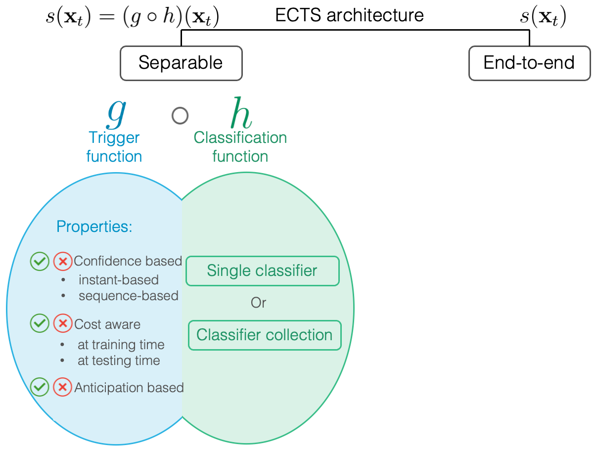
2.1 The different forms of the function
An ECTS function must solve both the question of (i) when to stop receiving new measurements and decide to make a prediction and (ii) how to make that prediction about the class of the incoming time series .
In the separable approaches, the two questions are solved using two separate components. The classification one deals with making a prediction: , while the trigger function decides when to predict. Within this approach, the classification component is learned independently of the trigger one, whereas the latter uses the results of the classification one in order to trigger a decision. A simple case is to decide it is time to make a prediction as soon as the prediction component is sufficiently sure of its prediction. We formalize separable approaches using the formula: where is the decision or trigger function, and is the prediction function.
In the end-to-end approaches, a single component decides when to make a prediction and what that prediction is. Thus, the function , defined in Equation 2, is responsible both for choosing the time for making the prediction, and for the prediction itself .
The question that naturally arises is which type of architecture (i.e. end-to-end or separable) performs best. On the one hand, in separable approaches, the classification component is trained independently of the triggering one, which can be detrimental. On the other hand, separating the ECTS problem into two inherently simpler sub-problems could be an advantage. In this paper, we do not delve any further into this question, which we leave for future work.
2.2 Choice of the optimizing criterion during training
This section covers optimization criteria existing in the literature and used to train ECTS functions. In the following, these criteria are listed by level of cost awarness, and we differentiate between the following situations:
-
1.
The first one, we call cost-aware at training time.
being unknown, instead of using Equation 3 describing the true risk, one tries to minimize the empirical risk, also called average cost in the ECTS literature, for a training set of time series:
(4) AvgCost is the most appropriate criterion to both train and evaluate ECTS approches. The following presents proxy measures of AvgCost.
-
2.
The second situation is a sub-case of cost-awareness, and can be qualified as cost-proxy at training time. There, while the accuracy and earliness of prediction are taken into account, the optimization criterion combines them in a proxy. Classical proxys include:
-
•
The Harmonic Mean (see (?)):
(5) with:
(6) (7) where is the time that the ECTS function decides to make prediction for the time series .
-
•
The CF (i.e. Cost Function) criterion with (see (?, ?, ?)):
(8) When the cost of misclassification , and the delay cost is and , CF becomes a particular case of AvgCost.
The choice of using costs or approximating them by a proxy is a technical issue, which may, for example, be relevant to making the loss function differentiable by approximation. For this reason, in the remainder of this paper, cost-aware/cost-proxys at training time situations are grouped together under the term cost-aware at training time, this difference not being essential.
-
•
-
3.
The third situation is qualified as cost-unaware-train. This is the case of methods that only set the threshold on the confidence of the prediction in order to trigger the prediction, regardless of the costs incurred on the training set. Another example is methods that use rigid rules, such as “decide as early as the first measurement is available”.
It is a question whether any of these approaches fare better than the others. To measure this, we must use the Average Cost (see Equation 4) measured on a test set, which represents the ground truth of the ECTS problem. It is to be remarked that many proposed methods were evaluated on other criteria in publications with the result of not allowing a rigorous comparison between them. We will come to this problem in Section 4.
The rest of this section is specific to separable ECTS approaches, which represent a large part of the literature.
2.3 Information used by the trigger function during inference
The trigger function can draw on different types of information. In the simplest case, it can decide irrespectively of the incoming time series . This is the case, for example, of the rule that would say: “wait until half of the measurements are available, then make a prediction”. The corresponding trigger function can be said to be blind.
Apart from this extreme case, it is interesting to distinguish two dimensions. First, the trigger function may or may not take the misclassification and delay costs into account. Second, it can also make its decision at each time step solely on the basis of past observations, or it can anticipate possible futures to help its decision.
For instance, confidence-based methods (seen Section 2.3.1) do not explicitly take costs into account in the triggering decision.
2.3.1 Confidence-based approaches
Confidence-based approaches are widely used in the literature. The simplest trigger model of this kind consists in monitoring a quantity related to the confidence of the prediction over time and triggering class prediction as soon as a threshold value is exceeded. The confidence metric monitored can take different forms. For example, a baseline approach, referred to as Proba Threshold 333Baseline implemented in the aeon library : https://urlz.fr/qmWl in the remainder of this paper, involves monitoring the highest conditional probability estimated by the classifier. This baseline example is referred as instant-based method, since it takes as input only the last confidence score available at time . Another type of approaches, referred as sequence-based, monitors the entire sequence of past confidence scores, and triggering a prediction is made conditionally on a particular property of this sequence. Finally, trigger functions can either take as input a scalar value, e.g. , in the case of instant based approaches, or a sequence of scalar values, e.g. , in the case of sequence-based approaches (see Section 3.1).
2.3.2 Cost-awareness at testing time
Given that an ECTS approach will ultimately be evaluated on the average cost of using it (see Equation 4), it seems natural to exploit the cost values at testing time, in order to trigger predictions at optimal moments. Method such as Economy (?) and 2step/NoCluster (?) do that. They can thus be qualified as “cost-aware at testing time”.
Other approaches use instead trigger functions that, once learned, do not take into account the cost at testing time, but that rely on other measures such as, for instance, the confidence of the prediction. This is the case of the SR approach (?). Therefore, these approaches can be qualified as “cost-unaware at testing time”.
Notice that some approaches are cost-aware during training but not during inference. This is the case with the SR approach, which is cost-aware at training time since it uses costs to optimize its parameters, and cost-unaware at testing time since the resulting trigger function does not use cost values during inference. Table 1 shows these two different properties for each approach in the literature.
2.3.3 Bling, Myopic and Anticipation-based decisions
Some separable approaches consider the output of the classifier at time to decide whether this is the right time to make a prediction. For instance, stopping the process when the confidence in the classification is above some threshold, or when the difference of confidence between the best two predictions exceeds some value. This type of method can be described as myopic since it only looks at the current time step , without trying to guess the future.
But there is a another possibility. As was first noted by ? (?), the ECTS problem can be cast as a LUPI (Learning Using Privileged Information) problem (?).
In this scenario, the learner can benefit at the training time of privileged information that will not be available at test time. Formally, the training set can be expressed as , where is what is observable and is some additional information not available when the prediction must be made. This is exactly what happens in the ECTS problem. Whereas at test time, only is available, during training the complete time series are known. This brings the possibility to learn what are the likely future of an incoming time series provided it comes from the same distribution. Hence, it becomes also possible to guess the cost to be optimized for all future time steps, and therefore to wait until the moment seems the best. This type of approach can be said anticipation-based (also called non-myopic in the literature). Because it exploits more information from the training set, it can be expected to outperform myopic and blind methods.
Is this confirmed by experience? Are there situations where the advantage is significant? Our experiments in Section 4 provide answers to these questions.
2.4 Choice of the classification component
One source of difficulty when devising a ECTS method in the separable setting is that inputs differ from one time step to another. The number of measurements, and hence the input dimension, varies. Two approaches have been used to deal with the problem.
-
1.
A set of classifiers is learned, each dedicated to a given time step , and thus a given input dimension. In practice, authors often chose a limited subset of timestamps, usually a set of twenty (one measurement every 5% of the length of the time series), to restrict the number of classifiers to learn and therefore the associated computational cost.
-
2.
A single classifier is used for all possible incoming time series . One way of doing this is to “project” an input of dimension , if is the dimension of an observation at time (i.e. multi-valued time series), into a fixed dimensional vector whatever and . This may simply be the mean value and standard deviation of the available measurements (multiplied by the dimension ) or the result of a more sophisticated feature engineering as tested by ? (?). Deep learning architectures can also be used to learn an encoding of the time series in an intermediate layer. For instance, ? (?) use a CNN architecture, and ? (?) a FCN one. ? (?) show that using deep neural architectures often perform well for time series classification.
Both approaches have their own limitations. On the one hand, using a set of classifiers, each independently dedicated to a time step, does not exploit information sharing. On the other hand, using a single classifier seems to be a more difficult task, as the representation of can be different at times and and all further time steps which can lead to additional difficulty for the classifier while moreover requiring a more demanding feature engineering step. Therefore, here also, it is interesting to measure experimentally whether one dominates the other. This will be the subject of future work.
3 State of the art
In this section, we position various existing proposed methods along the dimensions of the taxonomy presented in Section 2 (see Table 1). Then, we examine the methods and how they exemplify solutions to the general questions raised in the taxonomy. Thus, while each method combines solutions to all questions, in the following, we underline how each one brings an original solution to one specific problem. For instance, the Economy approach is separable, anticipation-based, and cost-aware at testing time. However, we’re focusing here on the anticipation-based dimension, since this is one of the first methods to have emphasized it and introduced an original solution for this aspect.
| References | Classifier(s) (collection ✓) | End2end | Confidence | Anticipation | Cost awareness |
|---|---|---|---|---|---|
| EDSC (?) | Shapelet | ✓ | ✓ | ✗ | |
| ECTS’ (?) | 1NN | ✓ | ✓ | ✗ | |
| Reject (?) | SVM | ✓ | ✗ | ||
| RelClass (?) | QDA, Linear SVM | ✓ | ✓ | ✗ | |
| \hdashlineiHMM (?) | HMM | ✓ | ✗ | ||
| 2step/NoCluster (?) | Linear SVM (✓) | ✓ | train & test | ||
| ECDIRE (?) | Gausian Process (✓) | ✓ | ✗ | ||
| Stopping Rule (?) | Gaussian Process (✓) | ✓ | train | ||
| \hdashlineEARLIEST (?) | LSTM | train | |||
| ECEC (?) | WEASEL (✓) | ✓ | train | ||
| DDQN (?) | MLP | ✓ | ✓ | train | |
| TEASER (?) | WEASEL (✓) | ✓ | train | ||
| \hdashlineECONOMY--max (?) | XGBoost tsfel (✓) | ✓ | train & test | ||
| DETSCNet (?) | TCN | ✓ | train | ||
| CALIMERA (?) | MiniROCKET (✓) | ✓ | train | ||
| ELECTS (?) | LSTM | ✓ | train | ||
| \hdashlineSOCN (?) | FCN | ✓ | train | ||
| EarlyStop-RL (?) | MLP | ✓ | ✓ | train |
3.1 Confidence-based approaches
Most ECTS methods to date are separable, confidence-based, cost-aware at training time, and are not anticipation-based. They implement separately the prediction and the triggering components, they learn them using the costs, hence they are cost-aware at training time, but they decide to trigger a decision based on the information available at the current time step without trying to anticipate the likely future, and they base their decision upon the confidence of the predictions made by the classifier.
There exist two families of confidence-based approaches. In the first one, only the last time step is considered, a score based on confidence estimations is monitored at each time step and a class prediction is triggered as soon as a threshold on this score is exceeded. By contrast, in the second, a sequence of estimated scores is monitored, and the condition to trigger a decision depends upon some property of this sequence.
3.1.1 Instant-based decision criterion
One basic method is to monitor , the highest conditional probability estimated by the classifier, which is a simple measure of classifier confidence over time. As soon as it exceeds a value, which is an hyper parameter of the method, a prediction is made. We call this method Proba_Threshold 444Baseline implemented in the aeon library : https://urlz.fr/qmWl and use it as baseline for comparison later in our experiments.
The Reject method (?) uses ensemble consensus as a confidence measure. For each time step, (i) first, a pool of classifiers is trained by varying their hyperparameters (i.e. SVMs); (ii) then, the most accurate of these are selected; (iii) and the pair of classifiers minimizing their agreement in predictions is chosen to form the ensemble. Finally, the prediction is triggered as soon as both classifiers in the ensemble predict the same class value. In this case, the monitored confidence measure is binary (agreement or disagreement), there is no trigger threshold and thus this trigger model is free of hyper-parameters 555The Reject approach involves choosing the number of classifiers trained in step (i) and selected in step (ii) that could be considered as hyper-parameters of the monitored confidence measure..
Hidden Markov Models (HMMs) are naturally suited to the classification of online sequences. An HMM is learned for each class, and at each time step , the class to be preferred is the one with the highest a posteriori probability given . However, the decision to make a prediction now or to postpone it must then involve a threshold so that the prediction is only made if the a posteriori probability of the best HMM is sufficiently high or is greater than that of the second-best. In reaction to this, ? (?) propose to replace the standard HMM with imprecise HMMs based on the concept of credal classifier. This eliminates the need to choose a threshold, since a decision is made when one classification “dominates” (according to a criterion based on probability intervals) all the others.
Rather that considering only the largest value predicted by the classifier, it is appealing to consider also the difference with the second largest value, since a large difference points to the fact that there is no tie between predictions to expect.
This is one dimension used in the Stopping Rule (SR) approach (?). Specifically, the output of the system is defined as:
| (9) |
where is the largest posterior probability estimated by the classifier , is the difference between the two largest posterior probabilities, and represents the proportion of the incoming time series at time . The parameters ; and are learned from the training set.
Using the same notations as SR, the Early Classification framework based on class DIscriminativeness and RELiability (ECDIRE) (?) finds the earliest timestamp for which a threshold applied on is reached (defined as in Equation 9). Then, the quantity is monitored, and a second threshold is applied to trigger the prediction.
A different class of methods relies on searching telltale representations of subsequences, such that if the incoming time sequence matches one or more of these representations, then its class can be predicted. Typically, these representations take the form of shapelets that discriminate well one class from the others (?). For instance, the Early Distinctive Shapelet Classification (EDSC) method learns a distance threshold for each shapelet, based on the computation of the Euclidean distance between the considered subsequence and all others valid subsequences in the training set (?). It selects a subset of them, based on a utility measure that combines precision and recall, weighted by the earliness. A prediction is made as soon as matches one of these shapelets well enough. Because this family of methods is computationally expensive, extensions have been developed to reduce the computational load (?, ?). Other extensions aimed at improving the reliability of the predictions reliability (?, ?), and tackling multivariate time series (?, ?, ?, ?).
3.1.2 Sequence-based decision criterion
Other approaches propose sequence-based confidence measures specifically designed for the ECTS problem.
The Effective Confidence-based Early Classification (ECEC) (?) proposes a confidence measure based on the sequence of predicted class values, from the first one observed to the current timestamp. At each time step, this approach exploits the precision of the classifier to estimate the probability for each possible class value of being correct if predicted. Then, assuming that successive class predictions are independent, the proposed confidence measure represents the probability that the last class prediction is correct given the sequence of predicted class values. The proposed confidence measure is monitored over time, and prediction is triggered if this measure exceeds a certain threshold tuned as the single hyper-parameter.
The Teaser (Two-tier Early and Accurate Series classifiER) (?) approach considers the problem of triggering or not a prediction as a classification task, the aim of which is to discriminate between correct and bad class predictions. As the authors point out, the balance of this classification task varies according to the time step considered . Indeed, assuming there is an information gain over time, there are fewer and fewer bad decisions as new measurements are received (or even no bad decisions after a while, i.e. for some datasets). To exploit this idea, a collection of one-class SVMs is used, learning hyper-spheres around the correct predictions for each time step. A prediction is triggered when it falls within these hyper-spheres for consecutive time steps ( being a parameter of the method).
The Second-Order Confidence Network approach (SOCN) (?) considers, as does Teaser, the same classification task aiming to discriminate between correct and bad predictions. To learn this task, a transformer (?) is used, taking as input the complete sequence of conditional probabilities estimated by the classifier , from the first time step, up to the current time step. A confidence threshold is learned by minimizing the same cost function as (?), and above which the prediction is considered reliable and therefore triggered.
3.2 Anticipation-based methods
One way of designing approaches that anticipate future measurements is to achieve classification of an incomplete time series while guaranteeing a minimum probability threshold according to which the same decision would be made on the complete series. This is the case of the Reliability Classification (RelClass) approach (?). Assuming that the measurements are i.i.d. and generated by a Gaussian process, this approach estimates the conditional probability of the entire time series given an incomplete realization and thus derives guarantees of the form:
where is a random variable associated with the complete times series, is a confidence threshold, and is the classifier learned over complete times series. At each time step , is evaluated and a prediction is triggered if this term becomes greater than the threshold , which is the only hyper-parameter to be tuned.
Another way of implementing anticipation-based approaches is to exploit the continuations of training time series, which are full-length. One of the first method for ECTS (?) has been derived into such an anticipation-based approach (?). The first, called Early Classification on Time Series (ECTS)(?), exploits the concept of Minimum Prediction Length (MPL), defined as the earliest time step for which the predicted label should not change for the incoming time series from to . This is estimated by looking for the 1NN of in the training set, and check whether from onward, its predicted label did not change. To be more robust, the MPL is defined based on clusters computed on full-length training time series to estimate the best decision time. The approach has been extended later on to speed up learning stage (?). This method looks in its own way at the likely future of - i.e. an incomplete time series belongs to a cluster whose continuations are known - and thus can be considered as an anticipation-based method.
? (?) present a method that claims explicitly to be “non myopic” in that a decision is taken at time only insofar as it seems that no better time for prediction is to be expected in the future. In order to do this, the family of Economy methods estimates the future cost expectation based on the incoming time series . This can be done since the training data consists of full-length time series and therefore a Learning Using Privileged Information (LUPI) (?) is possible.
More formaly, the objective is to trigger a decision when is minimal, with:
| (10) |
A tractable version of Equation 10 has been proposed by introducing an additional random variable which is the membership of to the groups of a partition :
| (11) |
In technical terms, training approaches from the Economy framework involve estimating the three probability terms of Equation 11, for the current time step , as well as for future time steps , with:
-
•
the probability of belonging to the groups ,
-
•
the prior probability of classes in each group,
-
•
the probability of predicting when the true class is within the group .
A key challenge in this framework is to design approaches achieving the most useful partition for predicting decision costs expectation.
In the first article which presents this framework (?), a method, called Economy-, is designed as follows. (i) A partition of training examples is first performed by a K-means algorithm ; (ii) then a simple model uses the Euclidean distance as a proxy of the probability that belongs to each group; (iii) the continuation of training time series within each group is exploited to predict the cost expectation for future time steps.
In order to avoid the clustering step with the associated choice of hyper parameters, (?) presented a variant called NoCluster which uses the 1 nearest neighbor in the training set in order to guess the likely future of .
Then, Economy- was introduced in (?) which relies on a supervised method to define a confidence-based partition of training time series. The algorithm, dedicated to binary classification problems, is designed as follows: (i) a collection of partitions is constructed by discretizing the output of each classifier into equal-frequency intervals, the groups thus formed correspond to confidence levels for each time step; (ii) at the current time , the incoming time series belongs to only one group, since the output of the classifier falls within a particular confidence level; (iii) then, a Markov chain model is trained to estimate the probabilities of the future time step confidence levels. Economy--max (?) generalizes this approach to multi-class problems, aggregating the multiple conditional probabilities in the classifiers’ output by using only the most probable class value.
Finally, Calimera (?) uses anticipation about the future from another perspective. Instead of trying to guess the likely continuation of which allows one to compute expected future costs, and therefore to wait until there seems no better time to make a prediction, their method is based on predicting directly the difference in cost between predicting the class now or wait at least one more time step. If this difference is positive, then it is better to postpone the prediction. They advocate furthermore, that a calibration step should intervene above the regression in order to make a decision.
3.3 Reinforcement Learning based methods
To learn an ECTS function, it is possible to use an agent that learns what to do by exploring the outcomes associated with different decision strategies as it interacts with the world. The ECTS problem can therefore be recast as a reinforcement learning (RL) problem.
In RL, an agent must learn to associate an action with each observable state so that the expected gain be maximized. Let us suppose that the agent-environment interactions break naturally into subsequences which we call episodes
At each time step , the agent perceives the environment’s state (i.e. ), choses an action (i.e. either make a prediction now and measure the gain , or postpone the decision and receive the next measurement ) according to its current policy , where is the probability that action is taken given the state .
The goal is for the agent to learn an optimal policy from sequences of interactions with its environment . This can be done by computing the utility function defined for all (state, action) pairs. By definition:
| (12) |
and the optimal policy can be derived from:
| (13) |
It suffices at each observed state to chose action such as:
| (14) |
One way to learn the function is using the Q-learning algorithm (?, ?) 666Note that other approaches are possible in the reinforcement learning scenario, like learning the utility function and using TD-learning, or even learning the policy directly. The Q-learning approach is however widely used. and its variants for continuous definition of environment’s states, such as Deep Q-learning (?).
In End-to-end approaches, only one function is responsible for both stopping and making a prediction about the class of whereas, in separable approaches involves two combined functions, respectively dedicated to triggering the prediction and to the classification itself. In the case of Reinforcement Learning based approaches, this distinction takes the following form:
-
1.
The separable approach. RL can be used to learn the Trigger function only, once the classifiers have been learnt. In that case, the set of actions at each time step is restricted to two elements: {‘decide now’, ‘postpone decision’}. The function evaluates for each state the expected gain for each of the two possibilities, allowing one to decide what to do at each time step.
-
2.
The End-to-End approach. RL can also be used to learn at once both when to trigger a prediction and what prediction to make. In principle, it suffices to extend the set of actions to , where there are classes. Either, the agent postpones the decision, or it predicts a class for the incoming time series .
In the literature, Reinforcement Learning-based ECTS approaches frequently include Deep Learning modules:
Separable RL approaches:
The Early and Adaptive Recurrent Label ESTimator (Earliest) uses a RNN architecture (?) to make the prediction and a Reinforcement Learning agent trained jointly using policy gradient, to trigger prediction or not. If prediction is triggered, the hidden representation given by the RNN is sent to a Discriminator, whose role is to predict a class, given this representation. The model has been extended for irregularly sampled time series (?). ? (?) extend the ECTS framework to channel filtering, using here also Reinforcement Learning.
End-to-end RL approaches:
? (?, ?) use a Deep Q-Network (?), alongside a specifically designed reward signal, encouraging the agent to find a good trade-off between earliness and accuracy. Those type of approaches also naturally extend to online setting where time series are not of fixed length. (?) introduce EarlytStop-RL, in which model-free RL is used to address the problem of early diagnosis of lung cancer.
3.4 Deep Learning based methods
Alongside the Reinforcement Learning based approaches, there exist deep learning methods that do not use RL.
The Decouple ETSC Network (Detscnet) (?) architecture leverages a gradient projection technique in order to jointly learn two sub-modules: one for variable-length series classification, the other for the early exiting task.
The End-to-end Learned Early Classification of Time Series method (Elects) leverages a LSTM architecture, adding a stopping prediction head to the network and adapting the loss function to promote good early predictions (?).
4 Experiments & Results
This section presents the extensive set of experiments carried out in order to provide a consistent and fair evaluation of a wide range of the existing literature’s methods. We first describe the experimental protocol used. We then turn to the experiments and their results. Figure 2 provides a synthetic view of the organization of these experiments.
-
•
Section 4.1 introduces the experimental protocol as well as the global evaluation methodologies.
-
•
In Section 4.2, the main state-of-the-art and the three baseline methods have been evaluated using a widely used cost setting, i.e. with a a binary balanced misclassification cost and a linear delay cost.
-
•
In Section 4.3, methods are evaluated in an anomaly detection scenario where the misclassification cost matrix is severely imbalanced, with false negatives being much more costly than false positives, and where the delay cost is no longer linear with time but exponentially increasing with time.
- •
.
The experiments presented here aim to evaluate the effects of design choices on method performance and thus to provide answers to the questions:
-
•
Do anticipation-based methods perform better than blind or myopic ones?
-
•
Do methods that are cost-aware for their decision (i.e. explicitly estimating costs) perform better than methods that are cost-unaware (e.g. confidence-based) (see Section 2.3.2).
-
•
How the various methods fare when modifying the form of the delay cost and/or the misclassification cost matrix?
-
•
Does -normalization distort the measured performance of the methods. Are some methods more prone to this?
4.1 Experimental Protocol
This section covers the shared part of the experimental protocol for all experiments irrespective of the choice of the cost functions (see Sections 4.2 and 4.3 for this).
4.1.1 Evaluation of the performance
The ECTS problem explicitly balances the pressure to make a correct prediction and a time pressure. The correctness of the prediction is measured by the misclassification cost where is the prediction and is the true class. The time pressure is sanctioned by a delay cost that is assumed to be positive and, in most applications, an increasing function of time. Sometimes, the two can be combined when the misclassification cost is function of the time : .
Therefore, for each test times series , an ECTS method incurs a cost assumed to be of the following additive form: , where is the time when the system decided to make a prediction, this prediction being .
For a test set of time series, the average cost of a method is:
| (15) |
This is accordingly the criterion with which we evaluated the methods in the experiments reported in this paper.
In addition, in order to assess how the methods adapt to various balances between the misclassification and the delay costs, we vary the settings of these costs by weighting them during training and testing. The performance of the methods is therefore evaluated using the weighted average cost, as defined in Equation 16, for different values of the costs balance , ranging from to , with a step:
| (16) |
Small values of correspond to a high delay cost and a small misclassification cost ; inversely, large values of give more weight to the misclassification cost with a lower delay cost.
4.1.2 Optimization of the parameters of the methods
We have optimized the parameters of all tested methods using AvgCost during training as the optimization criterion. Most of the methods rely on some simple validation grid-search, for which the bounds have been set according to the original published papers. When possible, granularity of the grid has been adapted to keep similar computation times between competitors. As well, default hyper-parameters have been kept constant compared to the original papers. There was one exception. Because the original version of Teaser uses the Harmonic Mean (see Section 2.2), we have kept this setting (the resulting method being Teaser), and we have added a variant called Teaser optimized using AvgCost.
4.1.3 Comparing the trigger methods
In order to carry out a fair comparison between the tested methods, we isolated as far as possible the triggering function, responsible for deciding when to stop receiving measurements, from the prediction one, responsible for predicting a label to the incoming time series. As advocated in (?), we have chosen the MiniROCKET algorithm (?) to be the base classifier for all methods. It is indeed recognized as among the best performing classifier in the Time Series classification literature as well as one of the fastest one.
Of course, distinguishing the decision component from the prediction one is only possible for the “separable” methods. In our experiments, we chose not evaluated “end-to-end” methods, leaving that for future work.
Trigger models: Nine trigger models were selected from the literature based on their usage and their performance 777The EDSC algorithm (?), even though available in the provided library, is not included in the following experiments, due to high space and time complexity (which hinders fair comparisons).
-
•
Economy--Max (?): triggers a decision if the predicted cost expectation is the lowest at time when compared with the expected cost for all future time steps (cf. Section 3.2, Anticipation-based).
-
•
Calimera (?): triggers a decision when a regressor model which predicts the difference between the current observed cost and the minimum cost in the future is negative (cf. Section 3.2, Anticipation-based).
-
•
Stopping Rule (?): uses a trigger function based on a linear combination of confidence estimates and a delay measure linear on time (cf. Section 3.1, Confidence-based).
-
•
Teaser (?): The trigger module consists of a collection of One Class SVM learned over the training set in order to isolate good predictions from bad ones. A prediction is triggered once consecutive predictions have been classified as ‘good’ by these OneClass SVM ( being tuned to maximize the harmonic mean between Earliness and Accuracy) (cf. Section 3.1, Confidence-based).
-
•
Teaser (?): Same algorithm as above. is now tuned maximizing the criterion, in order to allow the method to adapt to different cost settings.
-
•
Ecec (?): defines a confidence measure, based on the aggregated confidence of the predictions up to time , and triggers a prediction if it exceeds a threshold, tuned by explicit grid-search (cf. Section 3.1, Confidence-based).
-
•
Ecdire (?): determines “safe” timestamps, based on classifier performance, from which predictions about possible classes can be made. Predictions cannot be triggered if those timestamps have not been reached. In addition, the difference between the two highest predicted probabilities must also exceed a certain threshold. (cf. Section 3.1, Confidence-based).
-
•
Ects (?): computes the first time for which nearest neighbors of the incoming time series in the training set were given a label that did not change by the classifier (cf. Section 3.2, Anticipation-based).
All these methods have been re-implemented using Python, reproducing results close to published ones. Except the code for the Ects implementation, which has been taken from ? (?). Hyper-parameters are the ones chosen in the original published methods. Code to reproduce the experiments is available publicly at https://github.com/ML-EDM/papers_experiments/tree/main/ects_reloading.
Baselines: Furthermore, in order to evaluate the benefits, if any, of the various methods, it is telltale to compare them with simple ones. We chose three such baselines:
-
•
Asap (As Soon As Possible) always triggers a prediction at the first possible timestep.
-
•
Alap (As Late As Possible) always waits the complete series to trigger the prediction.
-
•
Proba Threshold is a natural, confidence-based, cost-aware at training time, baseline: it triggers a prediction if the estimated probability of the likeliest prediction exceeds some threshold, found by grid search (cf. Section 3.1, Confidence-based).
4.1.4 Calibration of the classifications
Like ? (?), we add a calibration step when learning the classifiers, i.e. Platt’s scaling (?). Indeed, as we are dealing with collections of independently trained classifiers, the prediction scores may not remain consistent with one another over the time dimension. However, the trigger methods usually have their parameters set with the same values for all time steps. This is the case, for example with the Proba Threshold approach. In addition, some approaches such as Calimera and Economy--Max exploit the estimated posterior probabilities to estimate the future cost expectation. It is therefore highly desirable for all classifiers, at all times, to have their output calibrated.
4.1.5 Datasets and training protocol
Datasets 888All original datasets of the paper can be downloaded, already prepared and splitted, from https://urlz.fr/qRqu: In order to be able to directly compare our results to past experiments, we first use the usual TSC datasets from the UCR Archive (?) with the default split. In total, we have used 77 datasets from the UCR Archive, i.e. the ones with enough training samples to satisfy our experimental protocol end-to-end (blue cylinder in Figure 2). In this way, most of the datasets used by either ? (?) and ? (?) or by ? (?) are contained in our experiments.
A second collection of non -normalized data sets is also provided. In this way, the associated potential information leakage is avoided (see Section 1). Any difference with the performance obtained on the -normalized data sets can thus signal the danger of -normalization with firm evidence. Considering the limited amount of non -normalized datasets within the UCR archive (?), we have decided to look for complementary new datasets so as to provide another collection of datasets. To this end, the Monash archive for extrinsic regression (?), provided 20 new time series datasets, for which we have discretized the the numerical target variable into binary classes based on a threshold value. For instance, if this threshold is equal to the median value of the regression target, the resulting classification datasets will be balanced in term of classes (as in Section 4.2). Note that this threshold can be chosen differently to get imbalanced datasets (as in Section 4.3.2), several thresholds could also be used to increase number of classes. As a result, we get a new set of classification tasks, as has recently been done by ? (?). Finally, 35 datasets have been gathered: 15 from the original archive and 20 from the Monash extrinsic regression archive. (orange cylinder in Figure 2).
Splitting strategy:
When not using predefined splits, the train sets are split into two distinct sets in a stratified fashion: a first one to train the different classifiers, corresponding to 60% of the training set and another one to train the trigger model, trained over the 40% left. The set used to train the classifiers, is itself split into two different sets in order to train calibrators, using 30% of the given data. Because of this procedure, we have been led to exclude some of the datasets, due to their limited training set size.
All the experiments have been performed using a linux operating machine, with an Intel Xeon E5-2650 2.20GHz (24-cores) and 252GB of RAM. Proceeding all datasets (including both blue and orange cylinders) over all competing approaches takes between 9-10 days, using MiniROCKET classifier, which is the most efficient tested.
4.2 Experiments with balanced misclassification and linear delay costs
This first setting is the one most widely used in the literature to date.
4.2.1 Cost definition
The misclassification cost is symmetrical and balanced, the delay cost is linear. They can be defined as follows:
Thus, for each dataset, the AvgCost is bounded between 0 and 1.
4.2.2 Results and analysis
For comparability reasons, this first set of experiments is analyzed over the classical ETSC benchmark used in the literature so far (blue cylinder in Figure 2). Results over the new, non -normalized, datasets can be found in Appendix B.
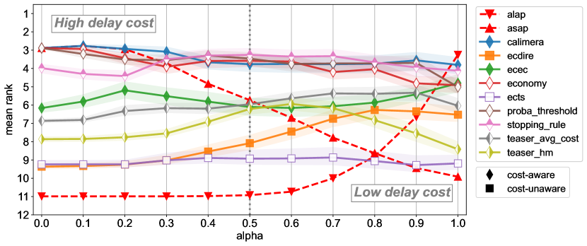
Figure 3(b) provides a global views about the relative performances of the tested methods. The Wilcoxon-Holm Ranked test provides an overall statistical analysis. It examines the critical difference among all techniques to plot the method’s average rank in a horizontal bar. Lower ranks denote better performance, and the methods connected by a horizontal bar are similar in terms of statistical significance. When evaluated by their average rank on all data sets with respect to the average cost (Equation 16), here for , four methods significantly outperform the others:
| Methods | Confidence | Anticipation | Cost awareness |
|---|---|---|---|
| Stopping Rule | ✓ | train | |
| Proba Threshold | ✓ | train | |
| Economy--max | ✓ | train & test | |
| Calimera | ✓ | train |
Figure 3(a) allows a closer look, this time varying the relative costs of misclassification and delaying prediction using Equation 16, where a small value of means that delay cost is paramount. level confidence intervals have been computed using bootstrap 999Resample with replacement has been done a large number of times (10.000 ) and are reported as shaded colors on the figure. The statistic of interest is studied, here the mean, by examining the bootstrap distribution at the desired confidence level.. Again, the same four methods top the others for almost every values of . Not surprisingly, the baseline Asap (predict as soon as possible) is very good when the delay cost is very high, while Alap (predict at time ) is very good when there is no cost associated with delaying decision.
It is remarkable that, in this cost setting, the simple Proba Threshold method exhibits a strong performance for almost all values of . It is therefore worth including in the evaluation of new methods. However, while Figures 3(a), 3(b) are useful for general analysis, they do not provide insights about how the Accuracy vs Earliness trade-off is optimized for each of the competitor. Figure 4 provides some explanation for this.
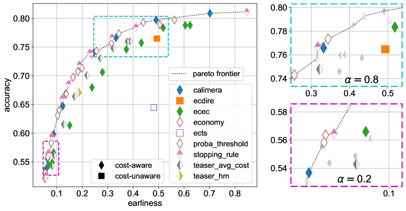
In this figure, the two evaluation measures: ‘Accuracy’ and ‘Earliness’, are considered as dimensions in conflict. The Pareto front is the set of points for which no other point dominates with respect to both Accuracy and Earliness. It is drawn here when varying their relative importance using (in the set ).
One must note first that, as Ects and Ecdire are cost-unaware, their performance do not vary with . Whatever the relative weight between accuracy and earliness, they make their prediction approximately after having observed half of the times series and they reach an average accuracy respectively near 0.64 and 0.77. They are clearly dominated by the other methods. This is also the case for Teaser, which, while being cost-aware at training time, also only appears once in the figure. Indeed, no weighting mechanism is provided in the original version of the algorithm, where the harmonic mean is used as an optimization criterion (see Equation 5).
Each of the leading methods Stopping Rule, Proba Threshold, Economy and Calimera have at least one point on the Pareto front and generally exhibits a combined performance very close to it. A closer look reveals how each approach optimizes the earliness vs. accuracy trade-off differently for a fixed cost. If we consider , for example, it appears that Economy takes its decision earlier than Proba Threshold, itself being more precocious than Ecec. Because this is also an area of problems where the delay cost is low, by doing so, Economy prevents itself from benefiting from waiting for more measurements and increasing its performance. Hence its slight downward slope on Figure 3(a) for high values of .
It’s worthnoting that the two naive baselines Asap and Alap perform better than the majority of approaches on seven values out of ten. This is specially the case when the delay cost is large, i.e. for , for which the Asap baseline is as competitive as top performers. Globally, the performance of Proba Threshold is remarkable in this cost setting. Even though, it is simply based on a single threshold on the confidence in the current prediction, its performance makes it one of the best methods. One question is how such simple method, like Proba Threshold, can adapt to scenarios where the misclassification and delay costs, not being symmetrical for the misclassification cost, and not linear for the delay one, reflect other application settings.
4.3 Experiments with unbalanced misclassification and non-linear delay costs
While the previous section has provided a first assessment of how the various methods adapt to different respective weights for the misclassification and the delay costs, it nonetheless assumed that the misclassification costs were balanced (e.g. 0 if correctly classified and 1 otherwise) and that the delay cost was a linear function of time.
There are however applications where these assumptions do not hold, for instance predictive maintenance or hospital emergency services, are characterized by (i) imbalanced misclassification costs (e.g. it is more costly to have to repair a machine than to carry out a maintenance operation that turns out not being necessary) and by (ii) non linear delay cost (e.g. usually, the later the surgical operation is decided, the costlier it is to organize it and the larger the risk for the patient). In the following, we call all applications presenting these characteristics “anomaly detection” applications.
The question arises as to how the various ECTS algorithms behave in this case, depending on their level of cost awareness and whether or not they are anticipation-based. This is what is investigated in the series of experiments reported in this section.
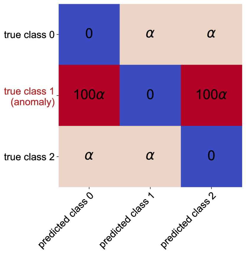
(three class problem)
4.3.1 Cost definition for anomaly detection
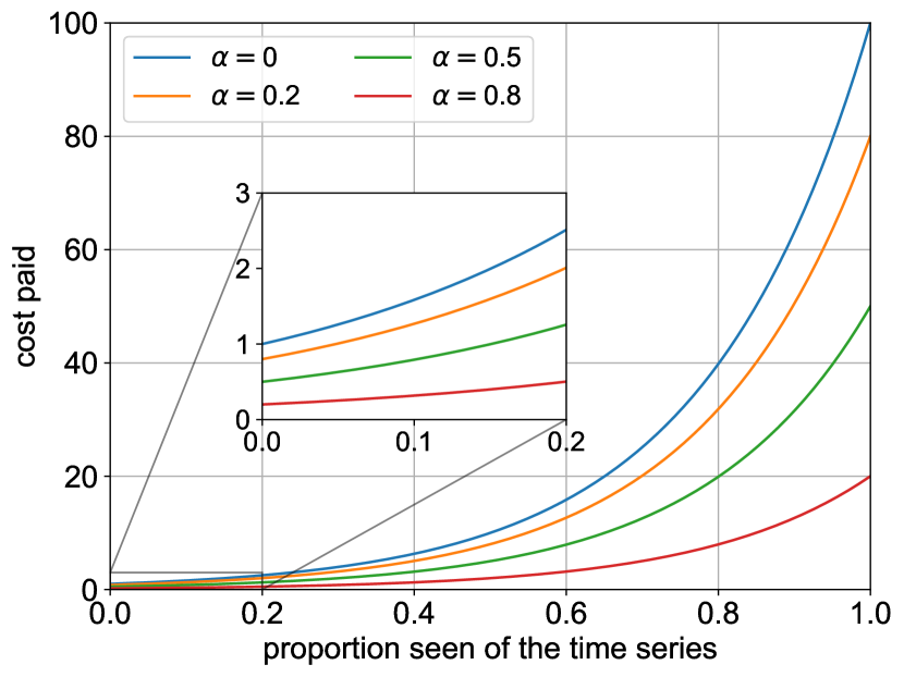
In order to study the behavior of the various algorithms on scenarios corresponding to anomaly detection, we set the unbalanced misclassification cost matrix such that a false negative (i.e. missing an anomaly) was 100 times costlier than a false positive (i.e. wrongly predicting an anomaly) (see Figure 5(b)). For this last situation, the cost was arbitrarily set to 1. The delay cost is defined as an exponential function of time. In order to have a cost commensurable with the misclassification one, we decided that waiting for the entire time series to be seen, at , would cost 100 (see Figure 5(a)), starting at 1 for and reaching 100 when .
4.3.2 Results and analysis
In this part, as a new cost setting is explored, there is no need to produce comparable results from previous works. Thus, we choose to use the new non -normalized datasets collection is now used (orange cylinder in Figure 2). In order for the imbalanced misclassification cost to make sense, those datasets have been altered so that minority class represents 20% of all labels. As explained in Section 4.1, some extrinsic regression datasets are turn into classification ones. In these cases, the threshold value has been set to the second decile of the regression target. For the original classification datasets, minority class has been sub-sampled when necessary.
figurec
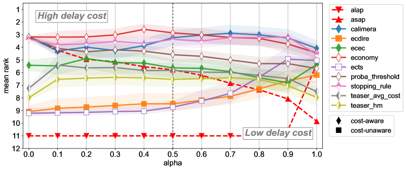

Results from the Wilcoxon-Holm Ranked test (both regarding the average rank and the value for AvgCost) (see Figure 6(b)) and from the AvgCost plot (see Figure 6(a)) with varying values of (in Equation 16) show that now the best method overall is Economy which is both cost-aware at training and testing time, and anticipating-based. However, Stopping-Rule is a very strong contender while being cost-aware at training time but not at testing time and confidence-based. There is a reason for it. When Stopping Rule equals or overpasses Economy, this is for high values of when the delay cost loses its importance, therefore leaving the misclassification cost to reign and confidence-based methods to be good.
It may come as a surprise that Calimera lags behind Economy for , despite being similarly based on the estimation of future cost expectation. One reason for this is that the cost expectation is achieved by considering only the predicted class. This poor estimate of the cost expectancy becomes critical when the delay cost is important.
Similarly, Proba Threshold is surprisingly good in this scenario, even if it is no longer in the top tier. Looking solely at prediction confidence, we might expect it to be blind to the rapid increase in delay cost in the anomaly detection scenario. However, it is noticeable that the cost of delay only increases sharply after around 60% of the complete time series has been observed, which is generally sufficient to exceed the confidence threshold. Hence, Proba Threshold does not suffer from high delay costs that are to come, and exhibits a good performance here.
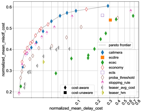
Figure 7 plots the Pareto front considering two axes based on decision costs. The horizontal axis corresponds to the average delay cost incurred for each example, normalized by the worst delay cost paid at . It is better to be on the left of the -axis. The vertical axis corresponds to 1 minus the misclassification cost incurred for each example, normalized by the worst prediction cost. It is better to be high on the -axis.
We observe that the Pareto front is composed almost exclusively of points corresponding to the Economy method. This is consistent with the evaluation based on the AvgCost metric. This figure highlights the fact that the design of approaches capable of handling arbitrarily parameterized decision costs requires a cost-aware application framework.
4.4 Other experiments: ablation and substitution studies
In the following Section, complementary experiments, such as ablation studies as well as sanity checks are briefly discussed. For conciseness, figures supporting the analysis can be found in Appendices B.
Impact of removing calibration
? (?) assert that calibration of the classifiers is paramount for the performance of ECTS algorithms. In order to test this claim, we have repeated the experiments removing the calibration step. The examples used for calibration have been removed as well during training, so that all else remains the same as before.
The results of Figure 11 show that indeed Calimera suffers greatly if no calibration is done. Indeed, this approach relies on estimating the expectation of future costs via a regression problem, and a miscalibration may have a negative impact on the built targets. For its part, Proba Threshold suffers somewhat mildly. This is no surprise as they rely on a single threshold on the confidence of the prediction for all time steps.
Impact of the choice of base classifier
All methods have been compared using the same classifier: MiniROCKET so that only the decision components differ. However, the choice of the base classifiers could induce a bias favoring or hampering some methods. In order to clarify this, we have repeated the experiments replacing MiniROCKET with two base classifiers: WEASEL 2.0 (?), and the XGBoost classifier (?) using features produced by tsfresh (?). Both of these classifiers have already been tested within the ECTS literature in (?, ?) and (?) respectively. Figure 12 and 13 in Appendix B report the results respectively with these two classification methods. One can observe that the results are not significantly altered with the same overall ordering of the method when varying the value of . Furthermore, our results on AvgCost show that performance tends to be better for all methods using MiniROCKET. It is thus to be preferred given its simplicity and good performance.
Impact of z-normalization
Considering the newly proposed ensemble of datasets, we were not able to identify any problems of information leakage over time. This inconclusive result simply indicates that the variance of the time series measurements is not informative for theses datasets, which still could be the case considering past published results. For further details, please refer to Section B.5 of Appendix B.
5 Conclusion
The first contribution of this research work is the coding of all the methods tested and making the codes available in a repository open to everyone. In this way, the experiments reported can be duplicated and further studies carried out. Furthermore, the deposited datasets and the experimental framework provide a ground for fair comparisons bewteen competing methods. We claim that the AvgCost is the appropriate measure by which to evaluate the performance of the methods. This is indeed what will be “paid” at the end of the day by a practitioner using a method. We have accordingly characterized a number of methods from the literature.
Our extensive experiments have shown that:
-
•
It is worthwhile to resort to dedicated ECTS methods, and more so in scenarios like anomaly detection with asymmetrical misclassification cost and exponential delay cost.
-
•
However, it is noticeable that Proba Threshold, a baseline method, is surprisingly good overall in the standard setting with symmetrical misclassification cost and linear delay cost, exhibiting comparable performance to confidence-based myopic methods such as Stopping-Rule and anticipation-based cost-aware ones such as Calimera and Economy.
-
•
Calibration of the classifiers has a large impact on some methods such as Calimera in particular, less so on other methods like Proba Threshold and Ecdire.
In this paper, we have proposed a reading guide to highlight the main characteristics of ECTS methods, namely (i) the importance of the two components: decision and prediction which are distinct in the “separable” architecture and not in the “end-to-end” one, (ii) the distinction between anticipation-based and myopic methods, and (iii) between cost-aware and cost-unaware techniques. On the basis of these dimensions, it becomes easy to imagine new methods that combine them in original ways, which could lead to new properties and better performance for solving the problem of early classification of time series, which, present in many applications has potentially great impacts.
To go a step further, future work could be carried out to study the literature’s approaches applied in as yet unexplored cost settings. For example, in many applications, the delay cost depends on the true class and the predicted one, and thus a single cost function integrating misclassification and delay costs should then be used. The use of this general cost form requires the adaptation of some state-of-the-art methods and has not yet been studied.
In addition, in real ECTS applications, it is up to the business expert to define the costs, which is not an easy task in practice. Future work could study the impact of: (i) noisy costs, (ii) and cost drift between training and testing stages. This would make it possible to identify the most resilient literature approaches.
Finally, in the case of existing separable approaches, misclassification cost is not exploited for training the classification function. Future work could investigate the interest of using cost-sensitive classifiers in the case of ECTS.
A Data description
A.1 UCR Time Series Classification datasets
| Train | Test | Length | Class | Type | |
| Data | |||||
| ACSF1 | 100 | 100 | 1460 | 10 | Device |
| Adiac | 390 | 391 | 176 | 37 | Image |
| Beef | 30 | 30 | 470 | 5 | Spectro |
| BeetleFly | 20 | 20 | 512 | 2 | Image |
| BME | 30 | 150 | 128 | 3 | Simulated |
| Car | 60 | 60 | 577 | 4 | Sensor |
| CBF | 30 | 900 | 128 | 3 | Simulated |
| Chinatown | 20 | 345 | 24 | 2 | Traffic |
| ChlorineConcentration | 467 | 3840 | 166 | 3 | Sensor |
| CinCECGTorso | 40 | 1380 | 1639 | 4 | Sensor |
| Coffee | 28 | 28 | 286 | 2 | Spectro |
| Computers | 250 | 250 | 720 | 2 | Device |
| CricketX | 390 | 390 | 300 | 12 | Motion |
| CricketY | 390 | 390 | 300 | 12 | Motion |
| CricketZ | 390 | 390 | 300 | 12 | Motion |
| Crop | 7200 | 16800 | 46 | 24 | Image |
| DiatomSizeReduction | 16 | 306 | 345 | 4 | Image |
| DistalPhalanxOutlineCorrect | 600 | 276 | 80 | 2 | Image |
| Earthquakes | 322 | 139 | 512 | 2 | Sensor |
| ECG200 | 100 | 100 | 96 | 2 | ECG |
| ECG5000 | 500 | 4500 | 140 | 5 | ECG |
| ECGFiveDays | 23 | 861 | 136 | 2 | ECG |
| ElectricDevices | 8926 | 7711 | 96 | 7 | Device |
| EOGVerticalSignal | 362 | 362 | 1250 | 12 | EOG |
| EthanolLevel | 504 | 500 | 1751 | 4 | Spectro |
| FaceAll | 560 | 1690 | 131 | 14 | Image |
| FaceFour | 24 | 88 | 350 | 4 | Image |
| FacesUCR | 200 | 2050 | 131 | 14 | Image |
| FiftyWords | 450 | 455 | 270 | 50 | Image |
| Fish | 175 | 175 | 463 | 7 | Image |
| FordA | 3601 | 1320 | 500 | 2 | Sensor |
| FreezerRegularTrain | 150 | 2850 | 301 | 2 | Sensor |
| GunPoint | 50 | 150 | 150 | 2 | Motion |
| Ham | 109 | 105 | 431 | 2 | Spectro |
| HandOutlines | 1000 | 370 | 2709 | 2 | Image |
| Haptics | 155 | 308 | 1092 | 5 | Motion |
| Herring | 64 | 64 | 512 | 2 | Image |
| HouseTwenty | 34 | 101 | 3000 | 2 | Device |
| InlineSkate | 100 | 550 | 1882 | 7 | Motion |
| InsectEPGRegularTrain | 62 | 249 | 601 | 3 | EPG |
| InsectWingbeatSound | 220 | 1980 | 256 | 11 | Sensor |
| ItalyPowerDemand | 67 | 1029 | 24 | 2 | Sensor |
| LargeKitchenAppliances | 375 | 375 | 720 | 3 | Device |
| Lightning2 | 60 | 61 | 637 | 2 | Sensor |
| Lightning7 | 70 | 73 | 319 | 7 | Sensor |
| Mallat | 55 | 2345 | 1024 | 8 | Simulated |
| Meat | 60 | 60 | 448 | 3 | Spectro |
| MedicalImages | 381 | 760 | 99 | 10 | Image |
| MelbournePedestrian | 1200 | 2450 | 24 | 10 | Traffic |
| MixedShapesRegularTrain | 500 | 2425 | 1024 | 5 | Image |
| MoteStrain | 20 | 1252 | 84 | 2 | Sensor |
| NonInvasiveFetalECGThorax1 | 1800 | 1965 | 750 | 42 | ECG |
| NonInvasiveFetalECGThorax2 | 1800 | 1965 | 750 | 42 | ECG |
| OSULeaf | 200 | 242 | 427 | 6 | Image |
| OliveOil | 30 | 30 | 570 | 4 | Spectro |
| PhalangesOutlinesCorrect | 1800 | 858 | 80 | 2 | Image |
| Plane | 105 | 105 | 144 | 7 | Sensor |
| PowerCons | 180 | 180 | 144 | 2 | Power |
| ProximalPhalanxOutlineCorrect | 600 | 291 | 80 | 2 | Image |
| RefrigerationDevices | 375 | 375 | 720 | 3 | Device |
| Rock | 20 | 50 | 2844 | 4 | Spectrum |
| ScreenType | 375 | 375 | 720 | 3 | Device |
| SemgHandGenderCh2 | 300 | 600 | 1500 | 2 | Spectrum |
| ShapesAll | 600 | 600 | 512 | 60 | Image |
| SmoothSubspace | 150 | 150 | 15 | 3 | Simulated |
| SonyAIBORobotSurface1 | 20 | 601 | 70 | 2 | Sensor |
| SonyAIBORobotSurface2 | 27 | 953 | 65 | 2 | Sensor |
| StarLightCurves | 1000 | 8236 | 1024 | 3 | Sensor |
| Strawberry | 613 | 370 | 235 | 2 | Spectro |
| SwedishLeaf | 500 | 625 | 128 | 15 | Image |
| Symbols | 25 | 995 | 398 | 6 | Image |
| SyntheticControl | 300 | 300 | 60 | 6 | Simulated |
| ToeSegmentation1 | 40 | 228 | 277 | 2 | Motion |
| Trace | 100 | 100 | 275 | 4 | Sensor |
| TwoLeadECG | 23 | 1139 | 82 | 2 | ECG |
| TwoPatterns | 1000 | 4000 | 128 | 4 | Simulated |
| UMD | 36 | 144 | 150 | 3 | Simulated |
| UWaveGestureLibraryX | 896 | 3582 | 315 | 8 | Motion |
| UWaveGestureLibraryY | 896 | 3582 | 315 | 8 | Motion |
| UWaveGestureLibraryZ | 896 | 3582 | 315 | 8 | Motion |
| Wafer | 1000 | 6164 | 152 | 2 | Sensor |
| Wine | 57 | 54 | 234 | 2 | Spectro |
| WordSynonyms | 267 | 638 | 270 | 25 | Image |
| Worms | 181 | 77 | 900 | 5 | Motion |
| Yoga | 300 | 3000 | 426 | 2 | Image |
A.2 Proposed, non -normalized, datasets
| Train | Test | Length | Class | Type | |
|---|---|---|---|---|---|
| Data | |||||
| \hdashlineBME | 30 | 150 | 128 | 3 | Simulated |
| Chinatown | 20 | 345 | 24 | 2 | Traffic |
| Crop | 7200 | 16800 | 46 | 24 | Image |
| DodgerLoopDay | 78 | 80 | 288 | 7 | Sensor |
| EOGVerticalSignal | 362 | 362 | 1250 | 12 | EOG |
| GestureMidAirD1 | 208 | 130 | 360 | 26 | Trajectory |
| GunPointAgeSpan | 135 | 316 | 150 | 2 | Motion |
| HouseTwenty | 34 | 101 | 3000 | 2 | Device |
| InsectEPGRegularTrain | 62 | 249 | 601 | 3 | EPG |
| MelbournePedestrian | 1200 | 2450 | 24 | 10 | Traffic |
| PLAID | 537 | 537 | Vary | 11 | Device |
| Rock | 20 | 50 | 2844 | 4 | Spectrum |
| SemgHandGenderCh2 | 300 | 600 | 1500 | 2 | Spectrum |
| SmoothSubspace | 150 | 150 | 15 | 3 | Simulated |
| UMD | 36 | 144 | 150 | 3 | Simulated |
| \hdashlineAcousticContaminationMadrid_nmv | 166 | 72 | 365 | 2 | Environnement |
| AluminiumConcentration | 440 | 189 | 2542 | 2 | Environnement |
| BitcoinSentiment | 232 | 100 | 24 | 2 | Sentiment |
| ChilledWaterPredictor | 321 | 138 | 168 | 2 | Energie |
| CopperConcentration | 440 | 189 | 2542 | 2 | Environnement |
| Covid19Andalusia | 142 | 62 | 91 | 2 | Santé |
| DailyOilGasPrices | 133 | 58 | 30 | 2 | Économie |
| DhakaHourlyAirQuality | 1447 | 621 | 24 | 2 | Environnement |
| ElectricityPredictor | 567 | 243 | 168 | 2 | Energie |
| FloodModeling3 | 429 | 184 | 266 | 2 | Environnement |
| HouseholdPowerConsumption1 | 1001 | 430 | 1440 | 2 | Energie |
| HotwaterPredictor | 245 | 106 | 168 | 2 | Energie |
| MadridPM10Quality_nmv | 4845 | 2077 | 168 | 2 | Environnement |
| ParkingBirmingham_eq | 1391 | 597 | 14 | 2 | Environnement |
| PrecipitationAndalusia_nmv | 470 | 202 | 365 | 2 | Environnement |
| SierraNevadaMountainsSnow | 350 | 150 | 30 | 2 | Environnement |
| SolarRadiationAndalusia_nmv | 470 | 202 | 365 | 2 | Energie |
| SteamPredictor | 210 | 90 | 168 | 2 | Energie |
| TetuanEnergyConsumption | 254 | 110 | 144 | 2 | Energie |
| WindTurbinePower | 596 | 256 | 144 | 2 | Energie |
B Supplementary results
B.1 Additional figures : Standard cost setting
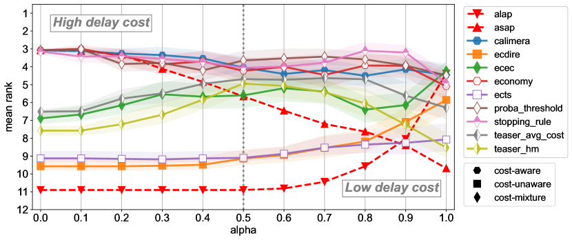
B.2 Additional figures : Anomaly detection cost setting
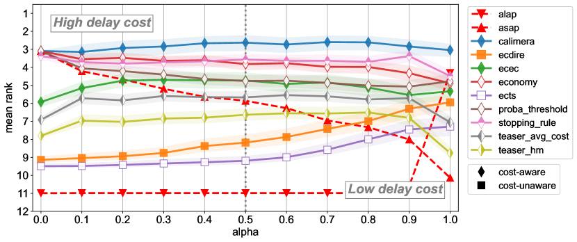
B.3 Removing calibration
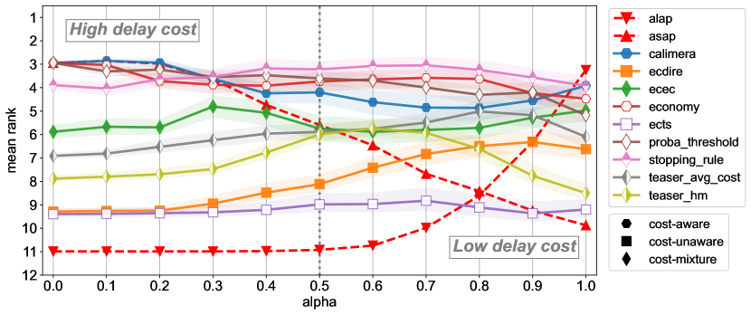
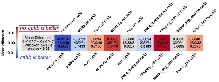
B.4 Changing the base classifier
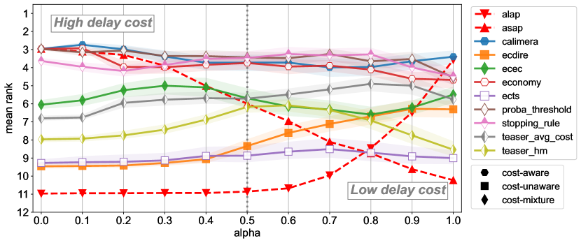
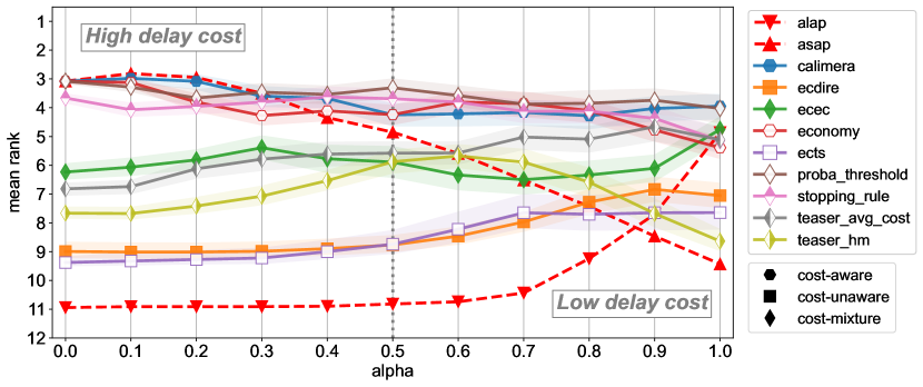
B.5 Impact of -normalization
For example, when a normalized time series has a low variance at the beginning, we can expect a high variance in the rest of the series since the mean variance is 1. There is therefore an information leakage that can be exploited by a ECTS algorithm, while this is not representative of what happens in real applications. A proposal such as the one presented in (?), where the Z-normalization of available time series is repeated at each time step, has its own problems. Besides being a costly solution, it means that if a single classifier is used for all time steps, the representation of can be different at times and and all further time steps which can induce confusion for the classifier.
On the one hand, -normalization induces an information leakage that could help methods to unduly exploit knowledge about the future of incoming time series. On the other hand, any normalization tends to smooth the signal and therefore, potentially, hinder the recognition of telltale features. So, does -normalization affect the performance of ECTS methods? And if yes, in which way? In order to answer this question, we took the new datasets collection described in Section 4.1. They are indeed not z-normalized originally. We duplicate and z-normalized them to get a second collection. As explained in Section 4.1, some extrinsic regression datasets has been converted into classification one. Here, the threshold value chosen to discretized the output into binary classes has been set the median of the regression target. In this way, classes within those datasets are equally populated.
In these experiments, the delay cost is linear as in Section 4.2 and as in most of the literature.
Figure 14 reports pairwise comparisons done on the 35 datasets. We look at , as this is the only value for which significant differences are observed. One can see that most of the trigger models do not actually benefit from the -normalization. Quite the opposite: out of nine trigger models, only one, i.e. Ecdire, actually has a better mean AvgCost when being trained on -normalized data. Regarding the remaining methods, both Stopping Rule and TeaserAvg performs significantly worse when operating on -normalized data. Those trends are quite similar for other values, without any significance on the statistical tests though. Thus, while -normalization has some impact, since privileged information from the future can be leaked, our experiments, for the proposed datasets collection at least, show that this does not alter the overall results reported in the literature, and are globally in accordance with the results presented in Section 4
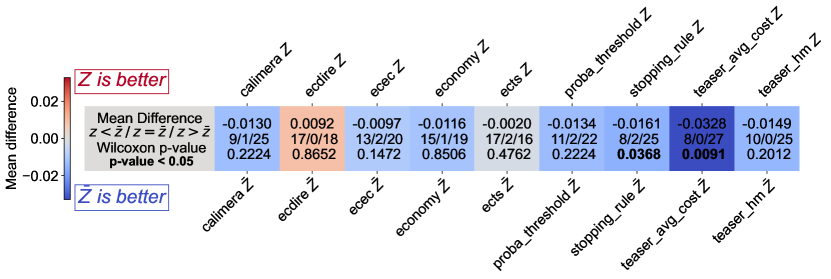
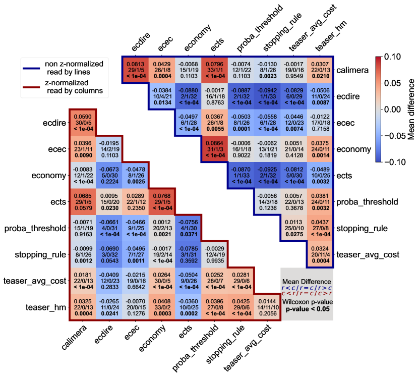
B.6 Anomaly detection cost setting : an ablation study
Exponential delay cost only
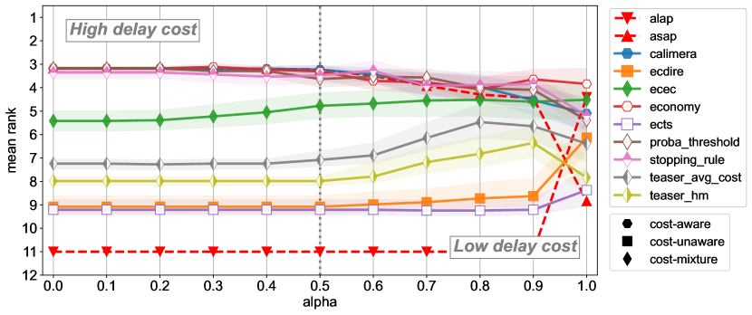
Imbalanced misclassification cost only
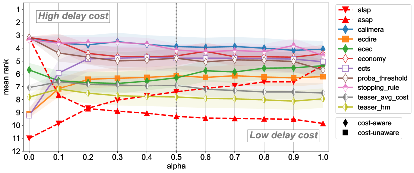
Standard cost setting, imbalanced datasets
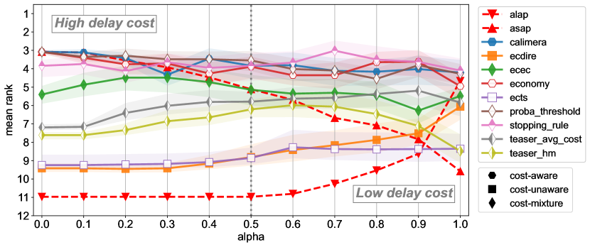
References
- Achenchabe et al. Achenchabe, Y., Bondu, A., Cornuéjols, A., and Dachraoui, A. (2021a). Early classification of time series: Cost-based optimization criterion and algorithms. Machine Learning, 110(6), 1481–1504.
- Achenchabe et al. Achenchabe, Y., Bondu, A., Cornuéjols, A., and Lemaire, V. (2021b). Early classification of time series is meaningful. arXiv preprint arXiv:2104.13257.
- Alonso González and Diez Alonso González, C. J., and Diez, J. J. R. (2004). Boosting interval-based literals: Variable length and early classification. In Data mining in time series databases, pp. 149–171. World Scientific.
- Antonucci et al. Antonucci, A., Scanagatta, M., Mauá, D. D., and de Campos, C. P. (2015). Early classification of time series by hidden markov models with set-valued parameters. In Proceedings of the NIPS time series workshop, pp. 1–5.
- Bilski and Jastrzebska Bilski, J. M., and Jastrzebska, A. (2023). Calimera: A new early time series classification method. Information Processing & Management, 60(5), 103465.
- Bondu et al. Bondu, A., Achenchabe, Y., Bifet, A., Clérot, F., Cornuéjols, A., Gama, J., Hébrail, G., Lemaire, V., and Marteau, P.-F. (2022). Open challenges for machine learning based early decision-making research. ACM SIGKDD Explorations Newsletter, 24(2), 12–31.
- Chen et al. Chen, H., Zhang, Y., Tian, A., Hou, Y., Ma, C., and Zhou, S. (2022). Decoupled early time series classification using varied-length feature augmentation and gradient projection technique. Entropy, 24(10), 1477.
- Chen et al. Chen, T., He, T., Benesty, M., Khotilovich, V., Tang, Y., Cho, H., Chen, K., Mitchell, R., Cano, I., Zhou, T., et al. (2015). Xgboost: extreme gradient boosting. R package version 0.4-2, 1(4), 1–4.
- Christ et al. Christ, M., Braun, N., Neuffer, J., and Kempa-Liehr, A. W. (2018). Time series feature extraction on basis of scalable hypothesis tests (tsfresh–a python package). Neurocomputing, 307, 72–77.
- Dachraoui et al. Dachraoui, A., Bondu, A., and Cornuéjols, A. (2013). Early classification of individual electricity consumptions. RealStream2013 (ECML), 18–21.
- Dau et al. Dau, H. A., Bagnall, A., Kamgar, K., Yeh, C.-C. M., Zhu, Y., Gharghabi, S., Ratanamahatana, C. A., and Keogh, E. (2019). The ucr time series archive. IEEE/CAA Journal of Automatica Sinica, 6(6), 1293–1305.
- Dayan and Watkins Dayan, P., and Watkins, C. (1992). Q-learning. Machine learning, 8(3), 279–292.
- Dempster et al. Dempster, A., Schmidt, D. F., and Webb, G. I. (2021). Minirocket: A very fast (almost) deterministic transform for time series classification. In Proceedings of the 27th ACM SIGKDD conference on knowledge discovery & data mining, pp. 248–257.
- Ferguson Ferguson, T. S. (1989). Who solved the secretary problem?. Statistical science, 4(3), 282–289.
- Ghalwash and Obradovic Ghalwash, M. F., and Obradovic, Z. (2012). Early classification of multivariate temporal observations by extraction of interpretable shapelets. BMC bioinformatics, 13, 1–12.
- Ghalwash et al. Ghalwash, M. F., Radosavljevic, V., and Obradovic, Z. (2014). Utilizing temporal patterns for estimating uncertainty in interpretable early decision making. In Proceedings of the 20th ACM SIGKDD international conference on Knowledge discovery and data mining, pp. 402–411.
- Gupta et al. Gupta, A., Gupta, H. P., Biswas, B., and Dutta, T. (2020). Approaches and applications of early classification of time series: A review. IEEE Transactions on Artificial Intelligence, 1(1), 47–61.
- Hartvigsen et al. Hartvigsen, T., Gerych, W., Thadajarassiri, J., Kong, X., and Rundensteiner, E. (2022). Stop&hop: Early classification of irregular time series. In Proceedings of the 31st ACM International Conference on Information & Knowledge Management, pp. 696–705.
- Hartvigsen et al. Hartvigsen, T., Sen, C., Kong, X., and Rundensteiner, E. (2019). Adaptive-halting policy network for early classification. In Proceedings of the 25th ACM SIGKDD International Conference on Knowledge Discovery & Data Mining, pp. 101–110.
- Hatami and Chira Hatami, N., and Chira, C. (2013). Classifiers with a reject option for early time-series classification. In 2013 IEEE symposium on computational intelligence and ensemble learning (CIEL), pp. 9–16. IEEE.
- He et al. He, G., Duan, Y., Peng, R., Jing, X., Qian, T., and Wang, L. (2015). Early classification on multivariate time series. Neurocomputing, 149, 777–787.
- He et al. He, G., Duan, Y., Qian, T., and Chen, X. (2013). Early prediction on imbalanced multivariate time series. In Proceedings of the 22nd ACM international conference on Information & Knowledge Management, pp. 1889–1892.
- Kladis et al. Kladis, E., Akasiadis, C., Michelioudakis, E., Alevizos, E., and Artikis, A. (2021). An empirical evaluation of early time-series classification algorithms.. In EDBT/ICDT Workshops.
- Klenke Klenke, A. (2013). Probability theory: a comprehensive course. Springer Science & Business Media.
- Lin et al. Lin, Y.-F., Chen, H.-H., Tseng, V. S., and Pei, J. (2015). Reliable early classification on multivariate time series with numerical and categorical attributes. In Advances in Knowledge Discovery and Data Mining: 19th Pacific-Asia Conference, PAKDD 2015, Ho Chi Minh City, Vietnam, May 19-22, 2015, Proceedings, Part I 19, pp. 199–211. Springer.
- Lv et al. Lv, J., Chu, Y., Hu, J., Li, P., and Hu, X. (2023). Second-order confidence network for early classification of time series. ACM Transactions on Intelligent Systems and Technology.
- Lv et al. Lv, J., Hu, X., Li, L., and Li, P. (2019). An effective confidence-based early classification of time series. IEEE Access, 7, 96113–96124.
- Martinez et al. Martinez, C., Perrin, G., Ramasso, E., and Rombaut, M. (2018). A deep reinforcement learning approach for early classification of time series. In 2018 26th European Signal Processing Conference (EUSIPCO), pp. 2030–2034. IEEE.
- Martinez et al. Martinez, C., Ramasso, E., Perrin, G., and Rombaut, M. (2020). Adaptive early classification of temporal sequences using deep reinforcement learning. Knowledge-Based Systems, 190, 105290.
- Mathukia et al. Mathukia, C., Fan, W., Vadyak, K., Biege, C., and Krishnamurthy, M. (2015). Modified early warning system improves patient safety and clinical outcomes in an academic community hospital. Journal of community hospital internal medicine perspectives, 5(2), 26716.
- Middlehurst et al. Middlehurst, M., Schäfer, P., and Bagnall, A. (2024). Bake off redux: a review and experimental evaluation of recent time series classification algorithms. Data Mining and Knowledge Discovery, 1–74.
- Mnih et al. Mnih, V., Kavukcuoglu, K., Silver, D., Rusu, A. A., Veness, J., Bellemare, M. G., Graves, A., Riedmiller, M., Fidjeland, A. K., Ostrovski, G., et al. (2015). Human-level control through deep reinforcement learning. nature, 518(7540), 529–533.
- Mori et al. Mori, U., Mendiburu, A., Dasgupta, S., and Lozano, J. A. (2017a). Early classification of time series by simultaneously optimizing the accuracy and earliness. IEEE transactions on neural networks and learning systems, 29(10), 4569–4578.
- Mori et al. Mori, U., Mendiburu, A., Keogh, E., and Lozano, J. A. (2017b). Reliable early classification of time series based on discriminating the classes over time. Data mining and knowledge discovery, 31, 233–263.
- Pantiskas et al. Pantiskas, L., Verstoep, K., Hoogendoorn, M., and Bal, H. (2023). Multivariate time series early classification across channel and time dimensions. arXiv preprint arXiv:2306.14606.
- Parrish et al. Parrish, N., Anderson, H. S., Gupta, M. R., and Hsiao, D. Y. (2013). Classifying with confidence from incomplete information. The Journal of Machine Learning Research, 14(1), 3561–3589.
- Platt et al. Platt, J., et al. (1999). Probabilistic outputs for support vector machines and comparisons to regularized likelihood methods. Advances in large margin classifiers, 10(3), 61–74.
- Rußwurm et al. Rußwurm, M., Courty, N., Emonet, R., Lefèvre, S., Tuia, D., and Tavenard, R. (2023). End-to-end learned early classification of time series for in-season crop type mapping. ISPRS Journal of Photogrammetry and Remote Sensing, 196, 445–456.
- Schäfer and Leser Schäfer, P., and Leser, U. (2020). Teaser: early and accurate time series classification. Data mining and knowledge discovery, 34(5), 1336–1362.
- Schäfer and Leser Schäfer, P., and Leser, U. (2023). Weasel 2.0: a random dilated dictionary transform for fast, accurate and memory constrained time series classification. Machine Learning, 112(12), 4763–4788.
- Shepp Shepp, L. A. (1969). Explicit solutions to some problems of optimal stopping. The Annals of Mathematical Statistics, 40(3), 993.
- Skakun et al. Skakun, S., Franch, B., Vermote, E., Roger, J.-C., Becker-Reshef, I., Justice, C., and Kussul, N. (2017). Early season large-area winter crop mapping using modis ndvi data, growing degree days information and a gaussian mixture model. Remote Sensing of Environment, 195, 244–258.
- Sutton and Barto Sutton, R. S., and Barto, A. G. (2018). Reinforcement learning: An introduction. MIT press.
- Tan et al. Tan, C. W., Bergmeir, C., Petitjean, F., and Webb, G. I. (2020). Monash university, uea, ucr time series extrinsic regression archive. arXiv preprint arXiv:2006.10996.
- Tavenard and Malinowski Tavenard, R., and Malinowski, S. (2016). Cost-aware early classification of time series. In Machine Learning and Knowledge Discovery in Databases: European Conference, ECML PKDD 2016, Riva del Garda, Italy, September 19-23, 2016, Proceedings, Part I 16, pp. 632–647. Springer.
- Vapnik and Vashist Vapnik, V., and Vashist, A. (2009). A new learning paradigm: Learning using privileged information. Neural networks, 22(5-6), 544–557.
- Vaswani et al. Vaswani, A., Shazeer, N., Parmar, N., Uszkoreit, J., Jones, L., Gomez, A. N., Kaiser, Ł., and Polosukhin, I. (2017). Attention is all you need. Advances in neural information processing systems, 30.
- Wang et al. Wang, W., Chen, C., Wang, W., Rai, P., and Carin, L. (2016). Earliness-aware deep convolutional networks for early time series classification. arXiv preprint arXiv:1611.04578.
- Wang et al. Wang, Y., Zhang, Q., Ying, L., and Zhou, C. (2024). Deep reinforcement learning for early diagnosis of lung cancer. In Proceedings of the AAAI Conference on Artificial Intelligence, Vol. 38, pp. 22410–22419.
- Wang et al. Wang, Z., Yan, W., and Oates, T. (2017). Time series classification from scratch with deep neural networks: A strong baseline. In 2017 International joint conference on neural networks (IJCNN), pp. 1578–1585. IEEE.
- Wu et al. Wu, R., Der, A., and Keogh, E. (2021). When is early classification of time series meaningful. IEEE Transactions on Knowledge and Data Engineering.
- Xing et al. Xing, Z., Pei, J., Dong, G., and Yu, P. S. (2008). Mining sequence classifiers for early prediction. In Proceedings of the 2008 SIAM international conference on data mining, pp. 644–655. SIAM.
- Xing et al. Xing, Z., Pei, J., and Philip, S. Y. (2009). Early prediction on time series: A nearest neighbor approach.. In IJCAI, pp. 1297–1302. Citeseer.
- Xing et al. Xing, Z., Pei, J., and Yu, P. S. (2012). Early classification on time series. Knowledge and information systems, 31, 105–127.
- Xing et al. Xing, Z., Pei, J., Yu, P. S., and Wang, K. (2011). Extracting interpretable features for early classification on time series. In Proceedings of the 2011 SIAM international conference on data mining, pp. 247–258. SIAM.
- Yan et al. Yan, W., Li, G., Wu, Z., Wang, S., and Yu, P. S. (2020). Extracting diverse-shapelets for early classification on time series. World Wide Web, 23, 3055–3081.
- Yao et al. Yao, L., Li, Y., Li, Y., Zhang, H., Huai, M., Gao, J., and Zhang, A. (2019). Dtec: Distance transformation based early time series classification. In Proceedings of the 2019 SIAM International Conference on Data Mining, pp. 486–494. SIAM.
- Ye and Keogh Ye, L., and Keogh, E. (2011). Time series shapelets: a novel technique that allows accurate, interpretable and fast classification. Data mining and knowledge discovery, 22, 149–182.
- Zafar et al. Zafar, P.-E., Achenchabe, Y., Bondu, A., Cornuéjols, A., and Lemaire, V. (2021). Early classification of time series: Cost-based multiclass algorithms. In 2021 IEEE 8th International Conference on Data Science and Advanced Analytics (DSAA), pp. 1–10. IEEE.
- Zhang and Wan Zhang, W., and Wan, Y. (2022). Early classification of time series based on trend segmentation and optimization cost function. Applied Intelligence, 1–12.