Re-examination of the role of displacement and photon catalysis operation in continuous variable measurement device-independent quantum key distribution

Abstract

We investigate the benefits of using $m$-photon catalysed two-mode squeezed coherent ($m$-PCTMSC) state in continuous variable measurement device-independent quantum key distribution (CV-MDI-QKD). To that end, we derive the Wigner characteristic function of the $m$-PCTMSC state and show that the 0-PCTMSC state is a Gaussian state and is an inferior choice as compared to the zero photon catalyzed two-mode squeezed vacuum state for CV-MDI-QKD. We carry out the optimization of the secret key rate with respect to all state parameters, namely variance, transmissivity, and displacement. Contrary to many recent proposals, the results show that zero- and single-photon catalysis operation provides only a marginal benefit in improving the maximum transmission distance. Secondly, we find that displacement offers no benefit in improving CV-MDI-QKD.

I Introduction

Quantum key distribution (QKD) has the capability to create a secure key shared between two parties despite transmitting data over an insecure quantum channel [1, 2, 3]. This security of QKD protocols is established by the fundamental principles of quantum mechanics. Discrete variable(DV) as well continuous variable(CV) quantum systems can be employed to carry out QKD [3]. Due to technical advantages, there has been significant increase in interest in CV QKD resulting in the rapid expansion of the field. Numerous CV-QKD protocols have undergone theoretical investigation and practical validation over the past two decades [3].

Inspired by the idea of entanglement swapping, measurement-device-independent QKD (MDI-QKD) protocol was proposed for discrete variable systems [4, 5]. The MDI-QKD protocols are immune to attack on detectors. The corresponding MDI-QKD for CV system was constructed and [6, 7, 8] several efforts have been made to enhance their efficiency in terms of maximum possible transmission distance over which secure QKD can be established.

Non-Gaussian operations have been shown to enhance the performance of quantum teleportation [9, 10, 11, 12, 13, 14, 15, 16], quantum metrology [17, 18, 19, 20, 21, 22, 23, 24, 25, 26] and quantum key distribution [27, 28, 29, 30]. Non-Gaussian operations such as photon subtraction, photon addition, and photon catalysis (PC) operations were considered in the context of CV-MDI-QKD operations [31, 32, 33, 34].

In this work, we consider the application of PC operation on the family of two mode squeezed coherent (TMSC) states and utilize them as resource states in CV-MDI-QKD. We first analytically derive the Wigner characteristic function of the $m$-photon catalyzed TMSC ($m$-PCTMSC) state, which is used to evaluate the covariance matrix. As a special case, we find that the Wigner characteristic function of the 0-PCTMSC state is Gaussian, while for higher values of $m$, the state is non-Gaussian. The Wigner characteristic function allows us to compute the covariance matrix required for the evaluation of the secret key rate for the protocol with $m$-PCTMSC state as the resource state. We optimized the secret key rate with respect to the state parameters, namely, variance, transmissivity, and displacement for a given value of $m$.

The results show that PC operations performed by Alice are not particularly useful and yield to only a marginal advantage. Displacement coupled with PC operation is not a useful operation as far as QKD is concerned, which is similar to our recent result on displacement coupled to photon subtraction [35]. In fact, the optimal variance for large distances is on the low range where both PC and displacement are not useful. These results are in contrast with several earlier pieces of published work [33, 34], where the advantage obtained was an artifact of working at high variance.

We were able to reach these conclusions because of our global approach and the fact that we had an analytical expression for the Wigner characteristic function for the $m$-PCTMSC state. Our results will directly impact other similar studies on photon catalysis such as virtual zero photon catalysis [36] and underwater CV-MDI-QKD [37].

The rest of the paper is organized in the following manner. In Sec. II, we commence by deriving the Wigner function of $m$-PCTMSC state. Section III introduces the $m$-PCTMSC state CV-MDI-QKD protocol. In Sec. IV, we present a detailed numerical simulation and optimize the secret key rate over the state parameters. Finally, Sec. V provides concluding remarks and future research directions.

II Wigner characteristic function and covariance matrix of the $m$-PCTMSC state

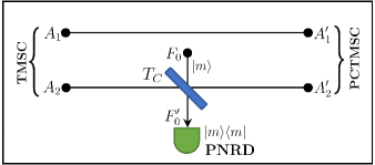
Figure 1: Schematic illustrating the generation of the PCTMSC state from the TMSC state. A beam splitter with transmissivity $T_{C}$ is used to interfere the ancillary mode $F_{0}$ in Fock state $|m\rangle$ and the mode $A_{2}$ of the TMSC state. An $m$-PCTMSC state is successfully generated when $m$ photons are detected by a photon number resolving detector.

The Wigner characteristic function corresponding to an $n$-mode quantum system state, as represented by the density operator $\hat{\rho}$, can be expressed as follows:

$$\chi(\Lambda)=\text{Tr}[\hat{\rho}\,\exp(-i\Lambda^{T}\Omega\hat{\xi})],\quad\Omega={\displaystyle\bigoplus_{k=1}^{n}}\begin{pmatrix}0&1\\ -1&0.\end{pmatrix}$$ (1)

where $\hat{\xi}=(\hat{q_{1}},\hat{p_{1}},\dots,\hat{q_{n}},\hat{p_{n}})^{T}$, and $\Lambda=(\Lambda_{1},\Lambda_{2},\dots,\Lambda_{n})^{T}$ with $\Lambda_{k}=(\tau_{k},\sigma_{k})^{T}\in\mathcal{R}^{2}$.

States with Gaussian Wigner characteristic function are known as Gaussian states. Such states can be uniquely specified via the first order moments and second order moments. First order moments is defined as $\bm{d}=\langle\hat{\xi}\rangle$. The second order moments can be written in the form of a matrix called covariance matrix $\Sigma$, whose entries are given by

$$(\Sigma)_{ij}=\frac{1}{2}\langle\{\hat{\xi_{i}},\hat{\xi_{j}}\}\rangle-\langle\hat{\xi_{i}}\rangle\langle\hat{\xi_{j}}\rangle.$$ (2)

Figure 1 shows the schematic for generating the PCTMSC state. We suppose that the modes $A_{1}$ and $A_{2}$ are initialized to the TMSC state. To generate TMSC state, we consider two uncorrelated modes, each of them initialized to a coherent state. Such a state is Gaussian and, therefore, can be described by the following displacement vector and covariance matrix (in shot noise units):

$$\bm{d}=(d,0,d,0)^{T},\quad\Sigma=\mathbb{1}_{4},$$ (3)

where $\mathbb{1}_{4}$ is the $4\times 4$ identity matrix. To generate a TMSC state, these modes are passed via a two-mode nonlinear optical down converter, whose effect can be modeled by the following symplectic transformation corresponding to two mode squeezing operation:

$$S_{A_{1}A_{2}}(\lambda)=\frac{1}{\sqrt{1-\lambda^{2}}}\begin{pmatrix}\,\mathbb{1}_{2}&\lambda\,\mathbb{Z}\\ \lambda\,\mathbb{Z}&\,\mathbb{1}_{2}\end{pmatrix},$$ (4)

where $\mathbb{Z}=\text{diag}(1,\,-1)$ and $\lambda=\tanh(r)$ with $r$ being the squeezing parameter. The displacement vector of the TMSC state can be evaluated as

$$\bm{d^{\prime}}=S_{A_{1}A_{2}}(\lambda)\bm{d}=\frac{d(1+\lambda)}{\sqrt{1-\lambda^{2}}}\begin{pmatrix}1\\ 0\\ 1\\ 0\\ \end{pmatrix}.$$ (5)

Similarly, the covariance matrix of the TMSC state can be calculated as

$$\Sigma^{\prime} =S_{A_{1}A_{2}}(\lambda)\Sigma S_{A_{1}A_{2}}(\lambda)^{T},$$ (6)

$$=\frac{1}{1-\lambda^{2}}\begin{pmatrix}(1+\lambda^{2})\,\mathbb{1}_{2}&2\lambda\,\mathbb{Z}\\ 2\lambda\,\mathbb{Z}&(1+\lambda^{2})\,\mathbb{1}_{2}\end{pmatrix}.$$

For the TMSC state, which is Gaussian and specified by the displacement vector (5) and covariance matrix (6), Eq. (1) acquires a simple form [38, 39]:

$$\chi(\Lambda)=\exp[-\frac{1}{2}\Lambda^{T}(\Omega\Sigma^{\prime}\Omega^{T})\Lambda-i(\Omega\bm{d^{\prime}})^{T}\Lambda].$$ (7)

Using the above equation, the Wigner characteristic function of the TMSC state, $\chi_{A_{1}A_{2}}(\Lambda_{1},\Lambda_{2})$, can be easily calculated. We consider an ancilla mode $F_{0}$ initialized to the Fock state $|m\rangle$. To interfere the mode $F_{0}$ with the mode $A_{2}$ of the TMSC state, a beam splitter with transmissivity $T_{C}$ is utilized. Before the interference, the Wigner characteristic function of the three mode system is given by

$$\chi_{A_{1}A_{2}F_{0}}(\Lambda)=\chi_{A_{1}A_{2}}(\Lambda_{1},\Lambda_{2})\chi_{|m\rangle}(\Lambda_{3}),$$ (8)

where $\chi_{|m\rangle}(\Lambda_{3})$ is the Wigner characteristic function of the Fock state:

$$\chi_{|m\rangle}(\Lambda_{3})=\exp\left[-\frac{\tau_{3}^{2}}{2}-\frac{\sigma_{3}^{2}}{2}\right]\,\mathcal{L}_{m}\left(\tau_{3}^{2}+\sigma_{3}^{2}\right),$$ (9)

where $\mathcal{L}_{m}(x)$ is the Laguerre polynomial. The three modes get entangled by the beam splitter’s action, and the modified Wigner characteristic function is given by

$$\chi_{A^{\prime}_{1}A^{\prime}_{2}F^{\prime}_{0}}(\Lambda)=\chi_{A_{1}A_{2}F_{0}}\left([\mathbb{1}\oplus B_{A_{2}F_{0}}(T_{C})]^{-1}\Lambda\right),$$ (10)

where $B_{A_{2}F_{0}}(T_{C})$ represents the beam splitter transformation given by

$$B_{A_{2}F_{0}}(T_{C})=\begin{pmatrix}\sqrt{T_{C}}\,\mathbb{1}&\sqrt{1-T_{C}}\,\mathbb{1}\\ -\sqrt{1-T_{C}}\,\mathbb{1}&\sqrt{T_{C}}\,\mathbb{1}\end{pmatrix}.$$ (11)

A photon number resolving detector is employed to measure the mode $F^{\prime}_{0}$. The measurement is described by the positive operator valued measure $\{\Pi_{m}=|m\rangle\langle m|,\mathbb{1}-\Pi_{m}\}$. The detection of $m$ photons indicates a successful $m$-photon catalysis operation. The unnormalized Wigner characteristic function of the $m$-PCTMSC state is

$$\widetilde{\chi}^{(m)}_{A_{1}A^{\prime}_{2}}(\Lambda_{1},\Lambda_{2})=\frac{1}{\pi}\int d^{2}\Lambda_{3}\,\chi_{A^{\prime}_{1}A^{\prime}_{2}F^{\prime}_{0}}(\Lambda)\chi_{|m\rangle}(-\Lambda_{3}).$$ (12)

II.1 Zero photon catalyzed TMSC state

We carry out a direct calculation of the integral (12) for $m=0$ to evaluate the Wigner characteristic function for 0-PCTMSC state:

$$\widetilde{\chi}^{(0)}_{A_{1}A^{\prime}_{2}}(\Lambda_{1},\Lambda_{2}) =\frac{\left(1-\lambda^{2}\right)}{1-\lambda^{2}T_{C}}\exp\left[-d^{2}\frac{(\lambda+1)^{2}\left(1-T_{C}\right)}{4\left(1-\lambda^{2}T_{C}\right)}\right]$$ (13)

$$\times\exp[-\frac{1}{2}\Lambda^{T}(\Omega\,\Sigma_{PC}^{(0)}\,\,\Omega^{T})\Lambda-i(\Omega\,\,\bm{d}_{PC}^{(0)})^{T}\Lambda],$$

where

$$\bm{d}_{PC}^{(0)}=\frac{d\sqrt{1-\lambda^{2}}}{1-\lambda^{2}T_{C}}\begin{pmatrix}(1+\lambda T_{C})\\ 0\\ (1+\lambda)\sqrt{T_{C}}\\ 0\\ \end{pmatrix},$$ (14)

and

$$\Sigma_{PC}^{(0)}=\frac{1}{1-\overline{\lambda}^{2}}\begin{pmatrix}(1+\overline{\lambda}^{2})\,\mathbb{1}_{2}&2\overline{\lambda}\,\mathbb{Z}\\ 2\overline{\lambda}\,\mathbb{Z}&(1+\overline{\lambda}^{2})\,\mathbb{1}_{2}\end{pmatrix},\quad\overline{\lambda}=\lambda\sqrt{T_{C}}.$$ (15)

The success probability of zero photon catalysis can be calculated from Eq. (13) as

$$P_{PC}^{(0)}=\widetilde{\chi}^{(0)}_{A_{1}A^{\prime}_{2}} (\Lambda_{1},\Lambda_{2})\bigg{|}_{\begin{subarray}{c}\tau_{1}=\sigma_{1}=0\\ \tau_{2}=\sigma_{2}=0\end{subarray}}=\frac{\left(1-\lambda^{2}\right)}{1-\lambda^{2}T_{C}}$$ (16)

$$\times\exp\left[-d^{2}\frac{(\lambda+1)^{2}\left(1-T_{C}\right)}{4\left(1-\lambda^{2}T_{C}\right)}\right].$$

Hence, the normalized Wigner characteristic function for 0-PCTMSC can be expressed as follows:

$$\chi^{(0)}_{A_{1}A_{2}^{\prime}}(\Lambda_{1},\Lambda_{2}) =\left(P_{PC}^{(0)}\right)^{-1}\widetilde{\chi}^{(0)}_{A_{1}A^{\prime}_{2}}(\Lambda_{1},\Lambda_{2}),$$ (17)

$$=\exp[-\frac{1}{2}\Lambda^{T}(\Omega\,\Sigma_{PC}^{(0)}\,\,\Omega^{T})\Lambda-i(\Omega\,\,\bm{d}_{PC}^{(0)})^{T}\Lambda].$$

Since the Wigner characteristic function is Gaussian, the 0-PCTMSC state is a Gaussian state with mean $\bm{d}_{PC}^{(0)}$ (14) and covariance matrix $\Sigma_{PC}^{(0)}$ (15). It is important to note that the covariance matrix of the 0-PCTMSC state (14) is independent of the displacement $d$. By substituting $d=0$ in the above equation, we can calculate the Wigner characteristic function for $0$-PCTMSV states. The form of the covariance matrix (15) suggests that the 0-PCTMSV state is another Gaussian state with a small variance. Additionally, if we take the limit of $T_{C}$ approaching unity in Eq. (17), we can obtain the Wigner characteristic function of the TMSC state.

The success probability for 0-PCTMSV can be obtained by setting $d=0$ in the above equation:

$$P_{PC}^{(0)}=\frac{\left(1-\lambda^{2}\right)}{1-\lambda^{2}T_{C}}.$$ (18)

Since

$$0\leq\frac{(\lambda+1)^{2}\left(1-T_{C}\right)}{4\left(1-\lambda^{2}T_{C}\right)}\leq 1,$$ (19)

the success probability of the 0-PCTMSC state is less than the 0-PCTMSV state. We would also like to remark that in Ref. [34], it has been claimed that the 0-PCTMSC state is a non-Gaussian state, which our explicit calculation shows is an incorrect statement.

II.2 Calculation for $m$-photon catalysis

To evaluate the integral (12) for the general case, we need to express the Laguerre polynomial present in the Wigner characteristic function of the Fock state $|m\rangle$ as follows:

$$\mathcal{L}_{m}\left(\tau_{3}^{2}+\sigma_{3}^{2}\right)=\frac{1}{m!}\frac{\partial^{2m}}{\partial u^{m}\partial v^{m}}e^{uv+u(\tau_{3}+i\sigma_{3})-v(\tau_{3}-i\sigma_{3})}\bigg{|}_{\begin{subarray}{c}u=0\\ v=0\end{subarray}}.$$ (20)

When the aforementioned equation is substituted in Eq. (12), a Gaussian integral is obtained that evaluates to

$$\widetilde{\chi}^{(m)}_{A_{1}A^{\prime}_{2}} =P_{PC}^{(0)}\chi^{(0)}_{A_{1}A_{2}^{\prime}}(\Lambda_{1},\Lambda_{2})$$ (21)

$$\times\bm{\widehat{D}}{\exp\big{[}-x_{1}u_{1}v_{1}+x_{2}u_{1}+x_{3}v_{1}-x_{4}u_{2}v_{2}}$$

$$+x_{5}u_{2}+x_{6}v_{2}+x_{7}(u_{1}v_{2}+v_{1}u_{2})\big{]},$$

where the coefficients $x_{i}$ are as under

$$x_{0}=(T_{C}\lambda^{2}-1)^{-1},\,\quad x_{1}=2x_{0}(1-T_{C}),$$

$$x_{2}=y_{0}+x_{0}y_{2},\quad\quad\quad x_{3}=y_{0}+x_{0}y_{3},$$

$$x_{4}=a_{4}\lambda^{2},\quad\quad\quad\quad\quad\,x_{5}=y_{1}+x_{0}y_{4},$$

$$x_{6}=y_{1}+x_{0}y_{5},\quad\quad\quad x_{7}=2x_{0}(\lambda^{2}-1)\sqrt{T_{C}},$$ (22)

with

$$y_{0}= x_{0}d(\lambda+1)\sqrt{1-\lambda^{2}}\sqrt{\left(1-T_{C}\right)T_{C}},$$ (23)

$$y_{1}= -x_{0}d(\lambda+1)\sqrt{1-\lambda^{2}}\sqrt{1-T_{C}}.$$

The operator $\bm{\widehat{D}}$ is given by

$$\bm{\widehat{D}}=\frac{1}{(m!)^{2}}\frac{\partial^{m}}{\partial\,u_{1}^{m}}\frac{\partial^{m}}{\partial\,v_{1}^{m}}\frac{\partial^{m}}{\partial\,u_{2}^{m}}\frac{\partial^{m}}{\partial\,v_{2}^{m}}\{\bullet\}_{\begin{subarray}{c}u_{1}=v_{1}=0\\ u_{2}=v_{2}=0\end{subarray}}.$$ (24)

The success probability of $m$-photon catalysis operation is evaluated from Eq. (21) as

$$P_{PC}^{(m)} =\widetilde{\chi}^{(m)}_{A_{1}A^{\prime}_{2}}(\Lambda_{1},\Lambda_{2})\bigg{|}_{\begin{subarray}{c}\tau_{1}=\sigma_{1}=0\\ \tau_{2}=\sigma_{2}=0\end{subarray}}$$ (25)

$$=P_{PC}^{(0)}\bm{\widehat{D}}{\exp\big{[}-x_{1}u_{1}v_{1}+y_{0}(u_{1}+v_{1})-x_{4}u_{2}v_{2}}$$

$$+y_{1}(u_{2}+v_{2})+x_{7}(u_{1}v_{2}+v_{1}u_{2})\big{]},$$

where the coefficients $y_{i}$ are given in Eq. (23). Finally, the normalized Wigner characteristic function of the $m$-PCTMSC state is given by

$$\chi^{(m)}_{A_{1}A_{2}^{\prime}}(\Lambda_{1},\Lambda_{2})=\left(P_{PS}^{(m)}\right)^{-1}\widetilde{\chi}^{(m)}_{A_{1}A^{\prime}_{2}}(\Lambda_{1},\Lambda_{2}).$$ (26)

Wigner characteristic function of PCTMSV states can be obtained by setting $d=0$ in the above equation. Further, in the limit $T_{C}\rightarrow 1$ in Eq. (26), we obtain the Wigner function of the TMSC state.

To evaluate the secret key rate, we need to compute the covariance matrix of the PCTMSC state [40]. The covariance matrix contains the averages of different symmetrically ordered operators. One of the major advantages of working in the Wigner characteristic formalism is that it is possible to determine the average of a symmetrically ordered operator by differentiating the $m$-PCTMSC state’s Wigner characteristic function with regard to the $\tau$ and $\sigma$ parameters as

$${}_{\bm{:}}^{\bm{:}}\hat{q_{1}}^{r_{1}}\hat{p_{1}}^{s_{1}}\hat{q_{2}}^{r_{2}}\hat{p_{2}}^{s_{2}}{}_{\bm{:}}^{\bm{:}}=\bm{\widehat{F}}\chi^{(m)}_{A_{1}A_{2}^{\prime}}(\tau_{1},\sigma_{1},\tau_{2},\sigma_{2}),$$ (27)

with

$$\bm{\widehat{F}}= \left(\frac{1}{i}\right)^{r_{1}+r_{2}}\left(\frac{1}{-i}\right)^{s_{1}+s_{2}}\frac{\partial^{r_{1}+s_{1}}}{\partial\sigma_{1}^{r_{1}}\partial\tau_{1}^{s_{1}}}$$ (28)

$$\times\frac{\partial^{r_{2}+s_{2}}}{\partial\sigma_{2}^{r_{2}}\partial\tau_{2}^{s_{2}}}\{\bullet\}_{\begin{subarray}{c}\tau_{1}=\sigma_{1}=0\\ \tau_{2}=\sigma_{2}=0\end{subarray}},$$

and the symbol ${}_{\bm{:}}^{\bm{:}}\bullet{}_{\bm{:}}^{\bm{:}}$ denotes Weyl ordering. By selecting appropriate values for $r_{1}$, $s_{1}$, $r_{2}$, $s_{2}$ in the Eq. (27), all the elements of the covariance matrix can be obtained. The covariance matrix takes the following specific form for the considered PCTMSC state:

$$\Sigma_{A_{1}A^{\prime}_{2}}=\begin{pmatrix}V_{A}^{q}&0&V_{C}^{q}&0\\ 0&V_{A}^{p}&0&V_{C}^{p}\\ V_{C}^{q}&0&V_{B}^{q}&0\\ 0&V_{C}^{p}&0&V_{B}^{p}\end{pmatrix}.$$ (29)

The covariance matrix for $m$-PCTMSC state ($m\geq 1$) does depend on the displacement.

III $m$-PCTMSC state based CV-MDI-QKD protocol

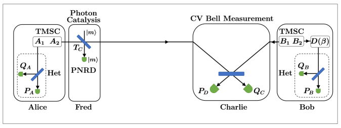
Figure 2: Schematic illustrating the working principle of CV-MDI-QKD protocol based on the PCTMSC state. To begin with, Alice and Bob prepare a TMSC state. Alice then transfers one of her modes to an unreliable party, Fred, to perform PC operation. The photon-catalyzed mode is then transferred to another unreliable party, Charlie, who uses a balanced beam splitter to combine it with the mode obtained from Bob. Charlie then executes homodyne measurement on the output modes and publishes the results. Based on the results, Bob performs a displacement operation, which entangles the modes with Alice and Bob. After that, Alice and Bob measure their modes using heterodyne measurement.

We introduce a CV-MDI-QKD protocol that is based on the $m$-PCTMSC state, with its schematic depicted in Fig. 2. The protocol involves two primary parties, Alice and Bob, who seek to establish a shared secure key. To achieve this, they undertake the methodology described below:

Step 1: Alice initializes a TMSC state with its two modes termed as $A_{1}$ and $A_{2}$. The variance of the state $V$, is fixed at $V=\cosh(2r)$.

Step 2: Alice sends one of the modes (say $A_{2}$) to Fred who implements the PC operation. The output mode($A^{\prime}_{2}$) is further transferred to Charlie through a quantum channel of length $L_{AC}$. This is done to facilitate entanglement swapping.

Step 3: Bob generates his own TMSC state with associated variance $V$. Let the two modes be denoted by $B_{1}$ and $B_{2}$. He then sends one of the modes ($B_{1}$) to Charlie via a separate quantum channel with length $L_{BC}$.

Step 4: Charlie utilizes a beam splitter to combine the received modes $A^{\prime}_{2}$ and $B_{1}$. Subsequently, he subjects the resulting output modes C and D, to homodyne measurements using $\hat{q}$ and $\hat{p}$ operators, and declares the respective measurement outcomes, $\{Q_{C},P_{D}\}$.

Step 5: Based on the results declared by Charlie, Bob applies a suitable displacement operation to his retained mode $B_{2}$, specifically $\hat{D}(g(Q_{C}+iP_{D}))$, with ‘$g$’ representing the gain factor. This transformation results in $B_{2}$ becoming $B^{\prime}_{2}$, effectively concluding the entanglement swapping process. The final state of modes $A_{1}$ and $B^{\prime}_{2}$ is entangled. Thereafter, Alice and Bob perform heterodyne measurements on their retained modes to obtain correlated outcomes, $\{Q_{A},P_{A}\}$ and $\{Q_{B},P_{B}\}$, respectively.

Step 6: The final step of CV-MDI-QKD is classical data post-processing, which involves information reconciliation (reverse reconciliation) and privacy amplification.

III.1 Secret key rate of PCTMSC based CV-MDI-QKD

We now calculate the secret key rate of the PCTMSC-based CV-MDI-QKD protocol. While the zero PC operation preserves the Gaussian character of the TMSC state, multi PC operation transforms the Gaussian state into a non-Gaussian state. We utilize the covariance matrix of the non-Gaussian state to calculate the secret key rate. This provides a lower bound on the secret key rate of the protocol with non-Gaussian states as the resource states [40].

As the CV-MDI-QKD protocol involves two quantum channels, Eve has the opportunity to employ two different methods for eavesdropping. In the first method, Eve carries out a correlated two-mode coherent Gaussian attack, introducing quantum correlations into both quantum channels, which is commonly referred to as the two-mode attack [41, 6]. In the second method, Eve independently implements entangling cloner attacks on each quantum channel, called as one-mode attack [6]. In our calculation of the secret key rate, we assume a one-mode collective Gaussian attack, which is a less effective eavesdropping strategy employed by Eve.

Since $L_{AC}$ and $L_{BC}$ are the transmission distances between Alice to Charlie and Bob to Charlie, the total transmission distance in the one-way CV-QKD protocol from Alice to Bob is $L_{AB}=L_{AC}+L_{BC}$. Here, the distance shall be expressed in kilometer (km). The quantum channel typically consists of an optical fiber network. The total loss in the optical fiber for a length $L$ is quantified as $\gamma L$, with $\gamma$ representing the attenuation factor in decibels per kilometer (dB/km) [42]. In this study, we adopt a value of $0.2$ dB/km for $\gamma$ [43].

Let the quantum channel between Alice and Charlie be characterized via the transmissivity $T_{A}$ and excess noise $\varepsilon_{A}^{\text{th}}$. Similarly, the quantum channel between Bob and Charlie is characterized via the transmissivity $T_{B}$ and excess noise $\varepsilon_{B}^{\text{th}}$. The length and transmissivities of these quantum channels are related by the relation $T_{A}=10^{-\gamma\frac{L_{AC}}{10}}$ and $T_{B}=10^{-\gamma\frac{L_{BC}}{10}}$.

Under the assumption that all of Bob’s operations, except for the heterodyne detection, are untrustable, the CV-MDI-QKD protocol under consideration becomes a one-way QKD protocol that makes use of heterodyne detection [44, 45, 7]. It is important to highlight that the secret key rate for this equivalent one-way QKD protocol is either less than or equal to the original protocol. We employ this one-way QKD protocol for the sake of simplifying our calculations when evaluating the secret key rate [46].

The corresponding transmissivity $T$ of the quantum channel in one-way QKD protocol can be given by $T=\frac{g^{2}}{2}T_{A}$, where $g$ represents the gain of the displacement operation implemented by Bob. Similarly, the corresponding excess noise $\varepsilon^{\text{th}}$ at optimal gain turns out to be

$$\varepsilon^{\text{th}}=\frac{T_{B}}{T_{A}}\left(\varepsilon_{B}^{\text{th}}-2\right)+\varepsilon_{A}^{\text{th}}+\frac{2}{T_{A}}.$$ (30)

Hence, the total channel-added noise turns out to be

$$\chi_{\text{ch}}=\frac{1-T}{T}+\varepsilon^{\text{th}}.$$ (31)

Using $I_{AB}$ to represent the mutual information between Alice and Bob and $\chi_{BE}$ to represent the Holevo bound between Bob and Eve, the secret key rate of the CV-MDI-QKD protocol can be expressed as

$$K=P^{(m)}_{PC}\left(\beta I_{AB}-\chi_{BE}\right).$$ (32)

Here $\beta$ represents the reconciliation efficiency. The calculation details for $I_{AB}$ and $\chi_{BE}$ are available in Refs. [31, 32]. The central point is that the covariance matrix elements are used to calculate the key rate in Eq.(32), which we can compute from the Wigner characteristic function described in Sec. II.

IV Numerical calculation and analysis of the secret key rate

Having computed the covariance matrix for the $m$-PCTMSC state, we now move on to numerically calculate the secret key rate for the family of $m$-PCTMSC states. Our focus will be on the extreme asymmetric case, when $L_{BC}=0$, i.e., Charlie and Bob are together as this scenario yields maximum transmission distance. Initially, we will discuss the secret key rate dependence on displacement for specific values of variance and transmissivity. Later, we will optimize the secret key rate with respect to PCTMSC state parameters, namely, variance, transmissivity, and displacement to obtain a global picture.

IV.1 The impact of displacement on transmission distance for PCTMSC states

In this section, we first scrutinize the effect of zero PC operation, wherein we explain the inherent limitations of the ‘0-PCTMSC state’ as compared to the ‘0-PCTMSV state’ and then move on to the non-Gaussian ‘1-PCTMSC state’, where we show that the right amount of displacement can substantially augment the performance for certain parameter value range.

IV.1.1 Secret key rate for 0-PCTMSC state

The covariance matrix of the 0-PCTMSC state is independent of the displacement, thereby rendering the factor $\left(\beta I_{AB}-\chi_{BE}\right)$ in the secret key rate (32) identical for both 0-PCTMSC and 0-PCTMSV states. However, as shown in Sec. II.1, the success probability for 0-PCTMSC state decreases with increasing displacement. Therefore, the secret key rate, which is a product of the probability and $\left(\beta I_{AB}-\chi_{BE}\right)$, of the 0-PCTMSC state is always less than 0-PCTMSV state. This, in turn, reduces the transmission distance when the displacement of the TMSC state is increased at a fixed secret key rate.

To understand how zero photon catalysis may appear to enhance the maximum transmission distance [33], two facts are important. Firstly, the fact that the 0-PCTMSV state is essentially another Gaussian state with a reduced variance as compared to the input state. Secondly, as presented in Fig. 3, if we plot variance as a function of maximum distance for a given key rate for the TMSV state, there is an optimal value of variance. Now, if the initial variance of the TMSV state is set higher than the optimal value, the 0-PC may lead to an increased value of the maximum transmission distance as it reduces the variance. This, however, is an artifact of working with a non-optimal value of variance and not a real advantage of zero photon catalysis. This is precisely the reason for the results shown in Ref. [33], a TMSV state with a variance of $V=15$ was considered, which revealed that zero photon catalysis could indeed enhance the maximum transmission distance. However, our findings, as illustrated in Fig. 6(c), indicate that when dealing with a TMSV state with smaller variance ($V=5$), zero photon catalysis does not lead to an increase in the transmission distance. The conclusion is that 0-PC is of no real use. In fact once it becomes clear that after 0-PC, the state is still a Gaussian state with deteriorated parameters, there is no question of this state giving any advantage over the initial state in any quantum protocol.

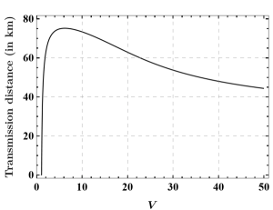
Figure 3: Transmission distance $L_{AB}$ as a function of variance $V$ at a fixed secret key rate $K=10^{-3}$ for the TMSV state. Numerical values of the other parameters are taken as $\beta=96\%$ and $\epsilon_{A}^{\text{th}}=\epsilon_{B}^{\text{th}}=0.002$.

There are several problems with the results presented in Ref. [34] in the context of zero photon catalysis; firstly, they have made a wrong conclusion that after zero photon catalysis the state becomes non-Gaussian; secondly, their graphs and text contain discrepancies on the role of displacement.

IV.1.2 Secret key rate for 1-PCTMSC state

We now turn to the analysis of 1-PCTMSC state and show that 1-PC operation on TMSV and TMSC states can have positive effects on the QKD performance. We first note that the performance of $1$-PCTMSC state is contingent on displacement since the covariance matrix depends on displacement. We analyze the variation in the maximum transmission distance as a function of displacement for 1-PCTMSC state at fixed secret key rate. The results are shown in Fig. 4, where we have considered a constant variance $V=15$ and three different values of transmissivities $T_{C}=0.90$, $0.94$, and $0.98$ at a fixed key rate $K=10^{-5}$.

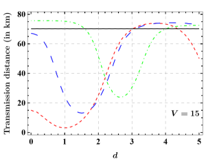
Figure 4: Transmission distance $L_{AB}$ as a function of displacement $d$ for different beam splitter transmissivities for the 1-PCTMSC state. The secret key rate is fixed at $K=10^{-5}$. Different curves for 1-PCTMSC state correspond to $T_{C}=0.90$ (dotted), $T_{C}=0.94$ ( dashed), and $T_{C}=0.98$ (dotdashed). The solid straight line represents the TMSV state. Numerical values of the other parameters are taken as $\beta=96\%$ and $\epsilon_{A}^{\text{th}}=\epsilon_{B}^{\text{th}}=0.002$.

The results show that 1-PC operation can have advantageous effects on TMSV state. Further, introducing displacement can lead to either beneficial or harmful outcomes depending on the transmissivity value. For instance, in the case of $T_{C}=0.90$, introducing displacement in the range of $d\in(3,4)$ yields optimal performance, outperforming the TMSV state. In Ref. [34] (Fig. 9), 1-PCTMSC state is shown to yield lower performance than the TMSV state at $d=2$, $V=50$, and $T_{C}=0.90$ . This is even evident in our result at $V=15$ for the curve $T_{C}=0.90$, where the performance is quite low at $d=2$. Therefore, introducing the right amount of displacement is crucial to achieving optimal performance. Furthermore, introducing displacement in the range $d\in(3.5,4.5)$ is beneficial while working at $T_{C}=0.94$. Finally, at $T_{C}=0.98$, displacement does not help in improving the transmission distance.

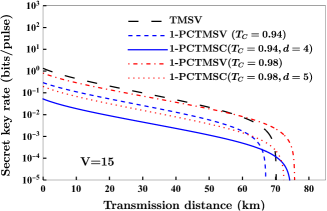
Figure 5: Secret key rate as a function of transmission distance. Numerical values of the other parameters are taken as $\beta=96\%$ and $\epsilon_{A}^{\text{th}}=\epsilon_{B}^{\text{th}}=0.002$.

These results can be explicitly seen in Fig. 5, where we plot the secret key rate as a function of transmission distance at fixed transmissivities and variance. At $T_{C}=0.94$, the maximum transmission distance of the 1-PCTMSV state is less than the TMSV state, while the maximum transmission distance of the 1-PCTMSC state is more than the TMSV state. On the other hand, at $T_{C}=0.98$, the maximum transmission distance for both 1-PCTMSV and 1-PCTMSC states is more than than the TMSV state; however, the maximum transmission distance of the 1-PCTMSV state is more than the 1-PCTMSC state.

We would like to point out that our results for 1-PC states like those for 0-PC state are at variance with the conclusions drawn in Ref. [34]. Secondly, as will become clear from the results in the next section and as was seen in the previous section, the advantage of displacement and PC are primarily in the high variance regime which is not the optimal value of variance.

IV.2 Optimization of the secret key rate with state parameters

The state parameters for PCTMSC states consist of variance which represents the amount of squeezing, displacement which represents the amplification factor, and transmissivity which represents the strength of the PC process. For the PCTMSV state, where displacement is set to zero, the state parameters are variance and transmissivity only. In an actual practical experimental situation where the experimentalist can generate a state with varying variance, displacement, and transmissivity, it is very important to find out what is the best of choice of these parameters for carrying out the QKD protocol. In such a scenario, we are interested in finding out the optimal value of parameters that maximizes the secret key rate of the QKD protocol. Two different situations are considered for the optimization of the secret key rate:

• Variance is kept fixed and the key rate is optimized with respect to displacement and transmissivity and cases of no PC, 0 PC and 1 PC.

• The key rate is optimized with respect to all the three parameters namely variance, displacement and transmissivity for the no PC 0 PC and 1 PC cases.

IV.2.1 Optimal displacement and transmissivity for fixed variance

We maximize the secret key rate by varying the displacement and transmissivity at a constant variance. We chose three difference values of the variance parameter namely, $V=5$, $V=10$, and $V=15$. The displacement parameter is restricted to the interval of $d\in(0,5)$. The optimization problem can be succinctly expressed as

$$\max_{d,T_{C}} K(V,d,T_{C})$$ (33)

subject to $$0\leq d\leq 5,$$

$$0\leq T_{C}\leq 1.$$

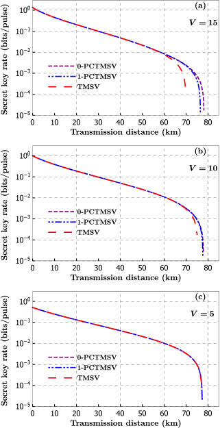
Figure 6: Secret key rate (optimized with respect to displacement and transmissivity) as a function of transmission distance. Three different variances have been considered: (a) $V=5$, (b) $V=10$, (c) $V=15$. Numerical values of the other parameters are taken as $\beta=96\%$ and $\epsilon_{A}^{\text{th}}=\epsilon_{B}^{\text{th}}=0.002$.

The optimization of state parameters is carried out for each transmission distance value. We only need to optimize the transmissivity parameter to achieve maximum secret key rate for the PCTMSV state. As expected, the optimal displacement for the 0-PCTMSC state turns out to be zero. Surprisingly, the optimal displacement for the 1-PCTMSC state is also zero. Since the optimal performance of the 0-PCTMSC and 1-PCTMSC states is the same as that of 0-PCTMSV and 1-PCTMSV states, respectively, we present the results only for 0-PCTMSV and 1-PCTMSV states along with the TMSV state in Fig. 6 for three fixed values of variance $(V=5$, $10$, and $15)$.

At high variance ($V=15$), both 0-PCTMSV and 1-PCTMSV states outperform the TMSV state. The maximum transmission distance is obtained for the 0-PCTMSV state followed by the 1-PCTMSV state. We note that this result for the 0-PCTMSV state has already been obtained in a previous study [33]. As the variance is decreased, all three states tend to yield the same performance. In particular, at $V=5$, we observe that the performance of the three states is similar. However, we also notice a decrease in the secret key rate as the variance decreases. It should be noted that the optimal transmissivity approaches unity wherever the PCTMSV states performance is equal to the TMSV state. This stems from the fact that the PCTMSV states approach the TMSV state in the unit transmissivity limit.

This leaves us with the task of finding the optimal variance of the employed resource states. The next section attempts to determine the optimal variance maximizing the secret key rate for different values of transmission distance.

IV.2.2 Optimal variance, displacement and transmissivity

We are now ready to we carry out the optimization of all state parameters, namely, variance, displacement, and transmissivity, with the aim of maximizing the secret key rate. The range of these parameters considered in the optimization is following:

$$\max_{V,d,T_{C}} K(V,d,T_{C})$$ (34)

subject to $$1\leq V\leq 15,$$

$$0\leq d\leq 5,$$

$$0\leq T_{C}\leq 1.$$

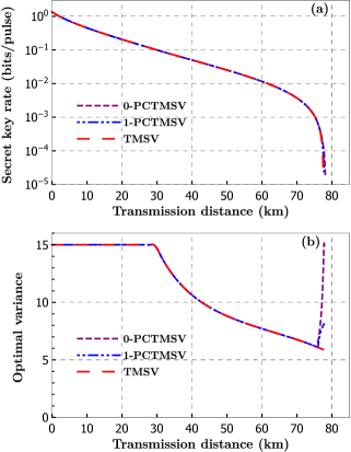
Figure 7: (a) Secret key rate (optimized with respect to variance, displacement, and transmissivity) as a function of the transmission distance. (b) Optimal variance as a function of the transmission distance. Numerical values of the other parameters are taken as $\beta=96\%$ and $\epsilon_{A}^{\text{th}}=\epsilon_{B}^{\text{th}}=0.002$.

The result of the optimization is shown in Fig. 7. We see that the PC operation can enhance the maximum transmission distance by less than one km. Further, the optimal variance is $V\approx 6$ at the maximum transmission distance; however, the optimal variance rises sharply for the 0-PCTMSV state. As states with low variances are easy to prepare, it raises a big question on the utility of photon catalysis by Alice in CV-MDI-QKD. Our analysis demonstrates that there is very little advantage in performance if Alice performs PC operations.

V Conclusion

In this article, we considered multiphoton catalysis on the TMSC state (the TMSV state is a special case). The generated state is used as a resource for CV-MDI-QKD. We showed that Alice’s implementation of zero and single photon catalysis has a negligible impact on enhancing the maximum transmission distance. Additionally, the results demonstrate that displacement does not yield any advantage in photon catalysis. The results provide a global perspective as we optimize all the state parameters and thereby show that many earlier results were artifacts of working in the wrong parameter regime. We presented our results stepwise so that we can make comparisons with earlier work.

A key ingredient of our work is that we computed the Wigner characteristic function of the PCTMSC states, which can be utilized to examine non-Gaussianity [47], nonlocality [48, 49], and nonclassicality [50, 51, 52]. In an earlier work [35], we demonstrated that applying photon subtraction on Alice’s end does not yield any benefits in CV-MDI-QKD. In future research, we aim to investigate whether noiseless linear amplifiers [53] and quantum scissors [54] can enhance the performance of CV-MDI-QKD.

Reference [34] claims that employing non-Gaussian operations on Bob’s side results in a final state with reduced entanglement content, potentially leading to a “lesser key rate or transmission distance”. However, Ref. [55] has demonstrated that entanglement content may be enhanced by performing non-Gaussian operation by Bob (after evolution through the noisy channel) as compared to non-Gaussian operation performed by Alice. Therefore, it is worthwhile to explore whether performing non-Gaussian operations on Bob’s side offers more advantages than doing so on Alice’s side.

References

- Gisin et al. [2002] N. Gisin, G. Ribordy, W. Tittel, and H. Zbinden, Quantum cryptography, Rev. Mod. Phys. 74, 145 (2002).
- Scarani et al. [2009] V. Scarani, H. Bechmann-Pasquinucci, N. J. Cerf, M. Dušek, N. Lütkenhaus, and M. Peev, The security of practical quantum key distribution, Rev. Mod. Phys. 81, 1301 (2009).
- Pirandola et al. [2020] S. Pirandola, U. L. Andersen, L. Banchi, M. Berta, D. Bunandar, R. Colbeck, D. Englund, T. Gehring, C. Lupo, C. Ottaviani, J. L. Pereira, M. Razavi, J. S. Shaari, M. Tomamichel, V. C. Usenko, G. Vallone, P. Villoresi, and P. Wallden, Advances in quantum cryptography, Adv. Opt. Photon. 12, 1012 (2020).
- Braunstein and Pirandola [2012] S. L. Braunstein and S. Pirandola, Side-channel-free quantum key distribution, Phys. Rev. Lett. 108, 130502 (2012).
- Lo et al. [2012] H.-K. Lo, M. Curty, and B. Qi, Measurement-device-independent quantum key distribution, Phys. Rev. Lett. 108, 130503 (2012).
- Pirandola et al. [2015] S. Pirandola, C. Ottaviani, G. Spedalieri, C. Weedbrook, S. L. Braunstein, S. Lloyd, T. Gehring, C. S. Jacobsen, and U. L. Andersen, High-rate measurement-device-independent quantum cryptography, Nature Photonics 9, 397 (2015).
- Li et al. [2014] Z. Li, Y.-C. Zhang, F. Xu, X. Peng, and H. Guo, Continuous-variable measurement-device-independent quantum key distribution, Phys. Rev. A 89, 052301 (2014).
- Ma et al. [2014] X.-C. Ma, S.-H. Sun, M.-S. Jiang, M. Gui, and L.-M. Liang, Gaussian-modulated coherent-state measurement-device-independent quantum key distribution, Phys. Rev. A 89, 042335 (2014).
- Opatrný et al. [2000] T. Opatrný, G. Kurizki, and D.-G. Welsch, Improvement on teleportation of continuous variables by photon subtraction via conditional measurement, Phys. Rev. A 61, 032302 (2000).
- Dell’Anno et al. [2007] F. Dell’Anno, S. De Siena, L. Albano, and F. Illuminati, Continuous-variable quantum teleportation with non-gaussian resources, Phys. Rev. A 76, 022301 (2007).
- Yang and Li [2009] Y. Yang and F.-L. Li, Entanglement properties of non-gaussian resources generated via photon subtraction and addition and continuous-variable quantum-teleportation improvement, Phys. Rev. A 80, 022315 (2009).
- Xu [2015] X.-x. Xu, Enhancing quantum entanglement and quantum teleportation for two-mode squeezed vacuum state by local quantum-optical catalysis, Phys. Rev. A 92, 012318 (2015).
- Hu et al. [2017] L. Hu, Z. Liao, and M. S. Zubairy, Continuous-variable entanglement via multiphoton catalysis, Phys. Rev. A 95, 012310 (2017).
- Wang et al. [2015] S. Wang, L.-L. Hou, X.-F. Chen, and X.-F. Xu, Continuous-variable quantum teleportation with non-gaussian entangled states generated via multiple-photon subtraction and addition, Phys. Rev. A 91, 063832 (2015).
- Kumar and Arora [2023] C. Kumar and S. Arora, Success probability and performance optimization in non-gaussian continuous-variable quantum teleportation, Phys. Rev. A 107, 012418 (2023).
- Kumar et al. [2024a] C. Kumar, M. Sharma, and S. Arora, Continuous variable quantum teleportation in a dissipative environment: Comparison of non-gaussian operations before and after noisy channel, Advanced Quantum Technologies 7, 2300344 (2024a).
- Birrittella et al. [2012] R. Birrittella, J. Mimih, and C. C. Gerry, Multiphoton quantum interference at a beam splitter and the approach to heisenberg-limited interferometry, Phys. Rev. A 86, 063828 (2012).
- Carranza and Gerry [2012] R. Carranza and C. C. Gerry, Photon-subtracted two-mode squeezed vacuum states and applications to quantum optical interferometry, J. Opt. Soc. Am. B 29, 2581 (2012).
- Braun et al. [2014] D. Braun, P. Jian, O. Pinel, and N. Treps, Precision measurements with photon-subtracted or photon-added gaussian states, Phys. Rev. A 90, 013821 (2014).
- Ouyang et al. [2016] Y. Ouyang, S. Wang, and L. Zhang, Quantum optical interferometry via the photon-added two-mode squeezed vacuum states, J. Opt. Soc. Am. B 33, 1373 (2016).
- Zhang et al. [2021] H. Zhang, W. Ye, C. Wei, Y. Xia, S. Chang, Z. Liao, and L. Hu, Improved phase sensitivity in a quantum optical interferometer based on multiphoton catalytic two-mode squeezed vacuum states, Phys. Rev. A 103, 013705 (2021).
- Tan et al. [2008] S.-H. Tan, B. I. Erkmen, V. Giovannetti, S. Guha, S. Lloyd, L. Maccone, S. Pirandola, and J. H. Shapiro, Quantum illumination with gaussian states, Phys. Rev. Lett. 101, 253601 (2008).
- Lopaeva et al. [2013] E. D. Lopaeva, I. Ruo Berchera, I. P. Degiovanni, S. Olivares, G. Brida, and M. Genovese, Experimental realization of quantum illumination, Phys. Rev. Lett. 110, 153603 (2013).
- Kumar et al. [2022] C. Kumar, Rishabh, and S. Arora, Realistic non-gaussian-operation scheme in parity-detection-based mach-zehnder quantum interferometry, Phys. Rev. A 105, 052437 (2022).
- Kumar et al. [2023a] C. Kumar, Rishabh, and S. Arora, Enhanced phase estimation in parity-detection-based mach–zehnder interferometer using non-gaussian two-mode squeezed thermal input state, Annalen der Physik 535, 2300117 (2023a).
- Kumar et al. [2023b] C. Kumar, Rishabh, M. Sharma, and S. Arora, Parity-detection-based mach-zehnder interferometry with coherent and non-gaussian squeezed vacuum states as inputs, Phys. Rev. A 108, 012605 (2023b).
- Huang et al. [2013] P. Huang, G. He, J. Fang, and G. Zeng, Performance improvement of continuous-variable quantum key distribution via photon subtraction, Phys. Rev. A 87, 012317 (2013).
- Guo et al. [2019] Y. Guo, W. Ye, H. Zhong, and Q. Liao, Continuous-variable quantum key distribution with non-gaussian quantum catalysis, Phys. Rev. A 99, 032327 (2019).
- Ye et al. [2019] W. Ye, H. Zhong, Q. Liao, D. Huang, L. Hu, and Y. Guo, Improvement of self-referenced continuous-variable quantum key distribution with quantum photon catalysis, Opt. Express 27, 17186 (2019).
- Hu et al. [2020] L. Hu, M. Al-amri, Z. Liao, and M. S. Zubairy, Continuous-variable quantum key distribution with non-gaussian operations, Phys. Rev. A 102, 012608 (2020).
- Ma et al. [2018] H.-X. Ma, P. Huang, D.-Y. Bai, S.-Y. Wang, W.-S. Bao, and G.-H. Zeng, Continuous-variable measurement-device-independent quantum key distribution with photon subtraction, Phys. Rev. A 97, 042329 (2018).
- Kumar et al. [2019] C. Kumar, J. Singh, S. Bose, and Arvind, Coherence-assisted non-gaussian measurement-device-independent quantum key distribution, Phys. Rev. A 100, 052329 (2019).
- Ye et al. [2020] W. Ye, H. Zhong, X. Wu, L. Hu, and Y. Guo, Continuous-variable measurement-device-independent quantum key distribution via quantum catalysis, Quantum Information Processing 19, 346 (2020).
- Singh and Bose [2021] J. Singh and S. Bose, Non-gaussian operations in measurement-device-independent quantum key distribution, Phys. Rev. A 104, 052605 (2021).
- Kumar et al. [2024b] C. Kumar, S. Chatterjee, and Arvind, Optimization of state parameters in displacement assisted photon subtracted measurement-device-independent quantum key distribution, arxiv.2406.04270 (2024b).
- Zhong et al. [2020] H. Zhong, Y. Guo, Y. Mao, W. Ye, and D. Huang, Virtual zero-photon catalysis for improving continuous-variable quantum key distribution via gaussian post-selection, Scientific Reports 10, 17526 (2020).
- Wang et al. [2020] Y. Wang, S. Zou, Y. Mao, and Y. Guo, Improving underwater continuous-variable measurement-device-independent quantum key distribution via zero-photon catalysis, Entropy 22, 10.3390/e22050571 (2020).
- Weedbrook et al. [2012] C. Weedbrook, S. Pirandola, R. García-Patrón, N. J. Cerf, T. C. Ralph, J. H. Shapiro, and S. Lloyd, Gaussian quantum information, Rev. Mod. Phys. 84, 621 (2012).
- Olivares [2012] S. Olivares, Quantum optics in the phase space, The European Physical Journal Special Topics 203, 3 (2012).
- García-Patrón and Cerf [2006] R. García-Patrón and N. J. Cerf, Unconditional optimality of gaussian attacks against continuous-variable quantum key distribution, Phys. Rev. Lett. 97, 190503 (2006).
- Ottaviani et al. [2015] C. Ottaviani, G. Spedalieri, S. L. Braunstein, and S. Pirandola, Continuous-variable quantum cryptography with an untrusted relay: Detailed security analysis of the symmetric configuration, Phys. Rev. A 91, 022320 (2015).
- Grasselli [2021] F. Grasselli, Beyond point-to-point quantum key distribution, in Quantum Cryptography: From Key Distribution to Conference Key Agreement (Springer International Publishing, Cham, 2021) pp. 83–104.
- Liao et al. [2017] S.-K. Liao, W.-Q. Cai, W.-Y. Liu, L. Zhang, Y. Li, J.-G. Ren, J. Yin, Q. Shen, Y. Cao, Z.-P. Li, F.-Z. Li, X.-W. Chen, L.-H. Sun, J.-J. Jia, J.-C. Wu, X.-J. Jiang, J.-F. Wang, Y.-M. Huang, Q. Wang, Y.-L. Zhou, L. Deng, T. Xi, L. Ma, T. Hu, Q. Zhang, Y.-A. Chen, N.-L. Liu, X.-B. Wang, Z.-C. Zhu, C.-Y. Lu, R. Shu, C.-Z. Peng, J.-Y. Wang, and J.-W. Pan, Satellite-to-ground quantum key distribution, Nature 549, 43 (2017).
- Grosshans et al. [2003] F. Grosshans, N. J. Cerf, J. Wenger, R. Tualle-Brouri, and P. Grangier, Virtual entanglement and reconciliation protocols for quantum cryptography with continuous variables, Quantum Info. Comput. 3, 535–552 (2003).
- Weedbrook et al. [2004] C. Weedbrook, A. M. Lance, W. P. Bowen, T. Symul, T. C. Ralph, and P. K. Lam, Quantum cryptography without switching, Phys. Rev. Lett. 93, 170504 (2004).
- Devetak and Winter [2005] I. Devetak and A. Winter, Distillation of secret key and entanglement from quantum states, Proceedings of the Royal Society A: Mathematical, Physical and Engineering Sciences 461, 207 (2005).
- Genoni et al. [2008] M. G. Genoni, M. G. A. Paris, and K. Banaszek, Quantifying the non-gaussian character of a quantum state by quantum relative entropy, Phys. Rev. A 78, 060303 (2008).
- Arvind and Mukunda [1999] Arvind and N. Mukunda, Bell’s inequalities, multiphoton states and phase space distributions, Physics Letters A 259, 421 (1999).
- Kumar et al. [2021] C. Kumar, G. Saxena, and Arvind, Continuous-variable clauser-horne bell-type inequality: A tool to unearth the nonlocality of continuous-variable quantum-optical systems, Phys. Rev. A 103, 042224 (2021).
- Hillery [1989] M. Hillery, Sum and difference squeezing of the electromagnetic field, Phys. Rev. A 40, 3147 (1989).
- Mandel [1979] L. Mandel, Sub-poissonian photon statistics in resonance fluorescence, Opt. Lett. 4, 205 (1979).
- Lee [1990] C. T. Lee, Many-photon antibunching in generalized pair coherent states, Phys. Rev. A 41, 1569 (1990).
- Jing et al. [2021] F. Jing, W. Liu, L. Kong, and C. He, Improving the performance of continuous-variable measurement-device-independent quantum key distribution via a noiseless linear amplifier, Entropy 23, 10.3390/e23121691 (2021).
- Kong et al. [2022] L. Kong, W. Liu, F. Jing, Z.-K. Zhang, J. Qi, and C. He, Improvement of a continuous-variable measurement-device-independent quantum key distribution system via quantum scissors, Chinese Physics B 31, 090304 (2022).
- Lee and Nha [2013] J. Lee and H. Nha, Entanglement distillation for continuous variables in a thermal environment: Effectiveness of a non-gaussian operation, Phys. Rev. A 87, 032307 (2013).