Extensions of Panjer’s recursion for mixed compound distributions

Abstract.

In actuarial practice, the usual independence assumptions for the collective risk model are often violated, implying a growing need for considering more general models that incorporate dependence. To this purpose, the present paper studies the mixed counterpart of the classical Panjer family of claim number distributions and their compound version, by allowing the parameters of the distributions to be viewed as random variables. Under the assumptions that the claim size process is conditionally i.i.d. and (conditionally) mutually independent of the claim counts, we provide a recursive algorithm for the computation of the probability mass function of the aggregate claim sizes. The case of a compound Panjer distribution with exchangeable claim sizes is also studied. For the sake of completeness, our results are illustrated by various numerical examples.

1. Introduction

Compound distributions are widely used in actuarial science for modelling the aggregate claims amount (denoted as $S$) paid by an insurance company over a fixed period of time. The computation of the probability distribution $P_{S}$ of $S$ is one of the main topics in the field. More formally, the random variable $S$ is defined as the random sum $S:=\sum_{n=1}^{N}X_{n}$, where $X:=\{X_{n}\}_{n\in{\mathbb{N}}}$ represents the individual claim sizes and $N$ is the random number of claims. Usually, the sequence $X$ is assumed to be independent and identically distributed and independent of $N$. Even under these independence assumptions, the determination of $P_{S}$ can be a difficult task, since one usually has to compute higher order convolutions. Consequently, recursive algorithms are often used for the computation of $P_{S}$.

One of the most prominent algorithms in actuarial literature is Panjer’s recursion (see Panjer (1981), Theorem, p. 24), which in the case of discrete claims size distribution simplifies the computation of the probability mass function (abbreviated as pmf) of $S$. Recall that the Panjer class of order $k\in{\mathbb{N}}_{0}$, denoted by ${\bf Panjer}(a,b;k)$, is a collection of claim number distributions $P_{N}=\{p_{n}\}_{n\in{\mathbb{N}}_{0}}$, satisfying $p_{n}=0$ for any $n\leq k-1$ and

$$p_{n}=\left(a+\frac{b}{n}\right)\cdot p_{n-1}\quad\text{ for all }n\geq k+1$$ (1)

(see Hess et al. (2002), p. 283). The members of the aforementioned class have been characterized by Sundt & Jewell (1981) for $k=0$, Willmot (1988) for $k=1$ and Hess et al. (2002) for a general $k\geq 2$. Recently, Fackler (2023) proposed a reparametrization for the members of the ${\bf Panjer}(a,b;k)$ class for $k\geq 0$ resulting in a more practical and unified representation of the corresponding probability distributions. More general recursive expressions than (1) have also been studied by Hesselager (1994), Schröter (1990), Sundt (1992) and Wang & Sobrero (1994). For an extensive review on recursive formulas for actuarial applications, we refer to Sundt & Vernic (2009) and the references therein.

In the case of inhomogeneous insurance portfolios, mixtures of claim number distributions are considered for modelling the claim counts. Gençtürk & Yiğiter (2016), Gómez-Déniz et al. (2004), Mansoor et al. (2020), Tzougas et al. (2019) and Wang (2011) proposed some (compound) mixed negative binomial distributions with different parametrizations using various mixing distributions. On the other hand, the literature for mixed Poisson and compound mixed Poisson distributions is much more enriched, encompassing, among others, the works of Antzoulakos & Chadjiconstantinidis (2004), Karlis & Xekalaki (2005), Nadarajah & Kotz (2006a, b), Sundt & Vernic (2004), Tzougas et al. (2021) and Willmot (1986, 1987). In particular, recursive formulas have been obtained by Willmot (1993) under the additional assumption that the logarithm of the induced (by the mixing distribution) probability density function can be written as the ratio of two polynomials. Moreover, by adopting the usual independence assumptions, Hesselager (1996) obtained a recursive formula for the computation of $P_{S}$.

In actuarial practice, the assumptions of independence among the random variables of $X$ and the mutual independence between $X$ and $N$ are often violated (see among others Albrecher & Boxma (2004), Albrecher & Teugels (2006) and Kolev & Paiva (2008)). In particular, the mutual independence assumption seems to be unrealistic, especially when considering inhomogeneous portfolios. This motivates us to consider a dependence structure among the random variables of $X$ and between $N$ and $X$. In contrast to the existing notion of compound (mixed) counting distributions, where the sequence $X$ is considered to be i.i.d. and mutually independent of $N$ (see Grandell (1997), Chapter 8, and Lyberopoulos & Macheras (2019), p. 4), in our case $X$ is only conditionally i.i.d. and conditionally mutually independent of $N$. This leads to the concept of mixed compound distributions (see Section 3), which constitute a strong generalization of compound (mixed) distributions.

Under the above framework, this work studies the mixed counterpart of the original ${\bf Panjer}(a,b;0)$ class and the corresponding compound distributions, by allowing the parameters of the claim number distribution $P_{N}$ to be measurable functions of a random vector, the claim size process $X$ to be conditionally i.i.d. and conditionally mutually independent of $N$. The above assumptions allow for a (possible) correlation (positive or negative) between $N$ and $X$, as well as correlation among the random variables of $X$. In addition, we consider the case of compound Panjer distributions with exchangeable claims. Henceforth, we denote by ${\bf Panjer}(a(\varTheta),b(\varTheta);0)$ the mixed Panjer class, where $\varTheta$ is a $d$-dimensional ($d\in{\mathbb{N}}$) random vector (also referred as structural parameter).

The rest of this paper is organized as follows. Section 2 provides a characterization for the members of ${\bf Panjer}(a(\varTheta),b(\varTheta);0)$ class in terms of regular conditional probabilities, and a recursive algorithm for the computation of their pmfSection 3 studies the probabilistic aspects of mixed compound distributions. Section 4 presents a recursive algorithm for the computation of $P_{S}$ in the case that $P_{N}\in{\bf Panjer}(a(\varTheta),b(\varTheta);0)$ and the claim size distribution is concentrated on ${\mathbb{N}}_{0}$. Numerical applications are also given in Section 4, whereas Section 5 concludes the paper.

2. The class of mixed Panjer claim number distributions

${\mathbb{N}}$ and ${\mathbb{R}}$ stand for the natural and the real numbers, respectively, while ${\mathbb{N}}_{0}:={\mathbb{N}}\cup\{0\}$ and ${\mathbb{R}}_{+}:=\{x\in{\mathbb{R}}:x\geq{0}\}$. If $d\in{\mathbb{N}}$, then ${\mathbb{R}}^{d}$ denotes the Euclidean space of dimension $d$. Given a topology $\mathfrak{T}$ on a set $\varUpsilon$, write ${\mathfrak{B}}(\varUpsilon)$ for its Borel $\sigma$-algebra on $\varUpsilon$, i.e., the $\sigma$-algebra generated by $\mathfrak{T}$. Also ${\mathfrak{B}}:={\mathfrak{B}}({\mathbb{R}})$ and ${\mathfrak{B}}(\alpha,\beta):={\mathfrak{B}}\big{(}(\alpha,\beta)\big{)}$, where $\alpha,\beta\in{\mathbb{R}}$ with $\alpha<\beta$, are the Borel $\sigma$-algebras of subsets of ${\mathbb{R}}$ and $(\alpha,\beta)$, respectively. For a non-empty set $A$, denote by $\mathbbm{1}_{A}$ and by $\mathcal{P}(A)$ its indicator function and its power set, respectively. Also, for a map $f:A\rightarrow{E}$ and a non-empty set $B\subseteq{A}$, write $f{\upharpoonright}B$ to denote the restriction of $f$ to $B$. Given two measurable spaces $(\varOmega,\varSigma)$ and $(\varUpsilon,T)$, as well as a $\varSigma$-$T$-measurable map $Z:\varOmega\to\varUpsilon$, denote by $\sigma(Z):=\{Z^{-1}[B]:B\in T\}$ the $\sigma$-algebra generated by $Z$.

Throughout what follows $(\varOmega,\varSigma,P)$ is an arbitrary probability space and $N$ is a random variable on $\varOmega$ taking values in a subset $R_{N}$ of  ${\mathbb{N}}_{0}$ containing $0$.

Sundt & Jewell (1981) proved that the only non-degenerate members of the original Panjer class of claim number distributions ${\bf Panjer}(a,b;0)$ are the Poisson, the binomial and the negative binomial distributions (see Sundt & Jewell (1981), Theorem 1). These distributions will be referred as basic claim number distributions. Since the members of ${\bf Panjer}(a,b;0)$ satisfy the recursive condition (1), an interesting question is whether their mixtures also satisfy a recursive relation. The previous question traces back to Sundt (1992), but for a more general family of claim number distributions, where it seems not to have a definite answer.

A way to model the mixtures of claim number distributions is to assume the existence of a random variable (or more generally of a random vector) $\varTheta$ on $\varOmega$ with values in $D\subseteq[0,\infty)$, such that the conditional distribution of $N$ given $\varTheta$ satisfies condition $P_{N\mid\varTheta}={\bf K}(\varTheta)$ $P{\upharpoonright}\sigma(\varTheta)$-almost surely (written a.s. for short), where ${\bf K}(\varTheta)$ is a conditional distribution (cf., e.g., Lyberopoulos et al. (2019), p. 455, for the definition of a conditional distribution). A claim number distribution $P_{N}$ that satisfies the previous condition is said to be a mixed claim number distribution. This motivates us to provide the following definitions within the class of mixed claim number distributions.

Definitions 2.1.

Let $\varTheta$ be a $d$-dimensional random vector with values in $D\subseteq{\mathbb{R}}^{d}$. A random variable $N$ is distributed according to:

(a) the mixed Poisson distribution with structural parameter $\xi(\varTheta)$ (written MP$\big{(}\xi(\varTheta)\big{)}$ for short), where $\xi$ is a ${\mathfrak{B}}(D)$-${\mathfrak{B}}({\mathbb{R}}_{+})$-measurable function, if

$$p_{n}(\varTheta):=P(N=n\mid\varTheta)=e^{-\xi(\varTheta)}\cdot\frac{\big{(}\xi(\varTheta)\big{)}^{n}}{n!}\quad P{\upharpoonright}\sigma(\varTheta)\text{-a.s.}$$

for any $n\in{\mathbb{N}}_{0}$;

(b) the mixed binomial distribution with structural parameters $z_{1}(\varTheta)$ and $z_{2}(\varTheta)$ (denoted by MB$\big{(}z_{1}(\varTheta),z_{2}(\varTheta)\big{)}$ for short), where $z_{1}$ and $z_{2}$ are ${\mathfrak{B}}(D)$-$\mathcal{P}({\mathbb{N}}_{0})$- and ${\mathfrak{B}}(D)$-${\mathfrak{B}}(0,1)$-measurable functions, respectively, if

$$p_{n}(\varTheta)=\binom{z_{1}(\varTheta)}{n}\cdot\big{(}z_{2}(\varTheta)\big{)}^{n}\cdot\big{(}1-z_{2}(\varTheta)\big{)}^{z_{1}(\varTheta)-n}\quad P{\upharpoonright}\sigma(\varTheta)\text{-a.s.}$$

for any $n\in\{0,1,\ldots,z_{1}(\varTheta)\}$ $P{\upharpoonright}\sigma(\varTheta)$-a.s.. In particular, if $z_{1}(\varTheta)$ or $z_{2}(\varTheta)$ is degenerate, simply write MB$\big{(}m,z_{2}(\varTheta)\big{)}$ ($m\in{\mathbb{N}}$) or MB$\big{(}z_{1}(\varTheta),p\big{)}$ ($p\in(0,1)$), respectively;

(c) the mixed negative binomial distribution with structural parameters $\rho_{1}(\varTheta)$ and $\rho_{2}(\varTheta)$ (written MNB$\big{(}\rho_{1}(\varTheta),\rho_{2}(\varTheta)\big{)}$ for short), where $\rho_{1}$ and $\rho_{2}$ are ${\mathfrak{B}}(D)$-${\mathfrak{B}}({\mathbb{R}}_{+})$- and ${\mathfrak{B}}(D)$-${\mathfrak{B}}(0,1)$-measurable functions, respectively, if

$$p_{n}(\varTheta)=\frac{\Gamma\big{(}\rho_{1}(\varTheta)+n\big{)}}{n!\cdot\Gamma\big{(}\rho_{1}(\varTheta)\big{)}}\cdot\big{(}\rho_{2}(\varTheta)\big{)}^{\rho_{1}(\varTheta)}\cdot\big{(}1-\rho_{2}(\varTheta)\big{)}^{n}\quad P{\upharpoonright}\sigma(\varTheta)\text{-a.s.}$$

for any $n\in{\mathbb{N}}_{0}$. In particular, if $\rho_{1}(\varTheta)$ or $\rho_{2}(\varTheta)$ is degenerate, simply write MNB$\big{(}r,\rho_{2}(\varTheta)\big{)}$ ($r>0$) or MNB$\big{(}\rho_{1}(\varTheta),p\big{)}$ ($p\in(0,1)$), respectively.

In what follows, unless stated otherwise, $\varTheta$ is a $d$-dimensional random vector with values in $D\subseteq{\mathbb{R}}^{d}$ and $\xi,z_{1},z_{2},\rho_{1}$ and $\rho_{2}$ are as in Definitions 2.1.

Definition 2.2.

A claim number distribution $P_{N}$ belongs to the class ${\bf Panjer}(a(\varTheta),b(\varTheta);0)$ if, the conditional distribution of $N$ given $\varTheta$ satisfies for every $n\in R_{N}\setminus\{0\}$ the condition

$$p_{n}(\varTheta)=\bigg{(}a(\varTheta)+\frac{b(\varTheta)}{n}\bigg{)}\cdot p_{n-1}(\varTheta)\quad P{\upharpoonright}\sigma(\varTheta)\text{-a.s.},$$ (2)

where $a$ and $b$ are real-valued ${\mathfrak{B}}(D)$-measurable functions.

Remarks 2.3.

(a) In the special case $P_{\varTheta}=\delta_{\theta_{0}}$, where $\delta_{\theta_{0}}$ denotes the Dirac measure concentrated on $\theta_{0}\in D$, the class ${\bf Panjer}(a(\theta_{0}),b(\theta_{0});0)$ coincides with the original Panjer class of claim number distributions.

(b) Recursive formulas for mixed claim number distributions can be found also in Gerhold et al. (2010), Lemma 5.7, but in a different context from condition (2). More precisely, these recursive formulas arise from a change of distributions technique for the mixing distribution.

Since the definition of ${\bf Panjer}(a(\varTheta),b(\varTheta);0)$ involves conditioning, it is natural to expect that the notion of regular conditional probabilities (also known as disintegrations) will play a crucial role in order to avoid trivialities and to treat conditioning in a rigorous way. The following definition is a special instance of Fremlin (2013), Definition 452E, appropriately adapted for our purposes (see also Lyberopoulos & Macheras (2021), Definition 3.1).

Definition 2.4.

Let $(\varUpsilon,T,Q)$ be a probability space. A family $\{P_{y}\}_{y\in\varUpsilon}$ of probability measures on $\varSigma$ is called a regular conditional probability (written rcp for short) of $P$ over $Q$ if

• for each $E\in\varSigma$ the map $y\mapsto P_{y}(E)$ is $T$-measurable;

• $\int P_{y}(E)\,Q(dy)=P(E)$ for each $E\in\varSigma$.

If $f:\varOmega\to\varUpsilon$ is an inverse-measure-preserving function (i.e., $P\big{(}f^{-1}[B]\big{)}=Q(B)$ for each $B\in T$), an rcp $\{P_{y}\}_{y\in\varUpsilon}$ of $P$ over $Q$ is called consistent with $f$ if, for each $B\in T$, the equality $P_{y}\big{(}f^{-1}[B]\big{)}=1$ holds for $Q$-almost all (written a.a. for short) $y\in B$.

The following result is taken from Lyberopoulos & Macheras (2012), and serves as a basic tool for the proofs of the upcoming results. In order to present it, denote by $\circ$ the function composition operator.

Lemma 2.5.

(Lyberopoulos & Macheras (2012), Lemma 3.5) Let $(\varUpsilon,T,Q)$ be a probability space and $f:\varOmega\to\varUpsilon$ be an inverse-measure-preserving function. Put $\sigma(f):=\{f^{-1}[B]:B\in T\}$ and suppose that an rcp $\{P_{y}\}_{y\in\varUpsilon}$ of $P$ over $Q$ consistent with $f$ exists. Then, for each $A\in\varSigma$ and $B\in T$ the following hold true:

1. $\mathbb{E}_{P}[g\mid\sigma(f)]=\mathbb{E}_{P_{\bullet}}[g]\circ f$ $P{\upharpoonright}\sigma(f)$-a.s., where $g$ is a $\varSigma$-$T$-measurable function such that $\int g\,dP$ is defined on ${\mathbb{R}}\cup\{-\infty,\infty\}$;

2. $\int_{B}P_{y}(A)\,Q(dy)=\int_{f^{-1}[B]}\mathbb{E}_{P}[\mathbbm{1}_{A}\mid\sigma(f)]\,dP=P\big{(}A\cap f^{-1}[B]\big{)}$.

Henceforth, $\{P_{\theta}\}_{\theta\in D}$ is an rcp of $P$ over $P_{\varTheta}$ consistent with $\varTheta$. For any $n\in R_{N}$ and $\theta\in D$, set $p_{n}(\theta):=P_{\theta}(N=n)$.

Remarks 2.6.

(a) The use of rcp’s in applied probability has been criticized mainly due to the fact that their existence is not always guaranteed (cf., e.g., Stoyanov (2013), Subsection 2.4). However, if $\varSigma$ is countably generated and $P$ is perfect (see Fremlin (2013), 451A(d), for the definition of a perfect measure), then there always exists an rcp $\{P_{y}\}_{y\in\varUpsilon}$ of $P$ over $Q$ consistent with every inverse-measure-preserving function $f$ from $\varOmega$ into $\varUpsilon$, provided that $T$ is also countably generated (see Faden (1985), Theorems 6 and 3). Note that the most important applications in actuarial science are still rooted in the case that $\varOmega$ is a Polish space (cf., e.g., Cohn (2013), p. 239, for its definition), where such rcp’s always exist. In particular, ${\mathbb{R}}^{d}$ and ${\mathbb{R}}^{{\mathbb{N}}}$ are typical examples of Polish spaces appearing in applications (see also Lyberopoulos & Macheras (2021), Remark 3.2). For an excellent review on rcp’s and their applications, we refer the interested reader to Chang & Pollard (1997).

(b) Each of the probability measures $P_{\theta}$ of the corresponding rcp can be interpreted as a version of the conditional probability $P(\bullet\mid\varTheta=\theta)$, which is well-defined, up to an a.s. equivalence, as a function of $\theta$, while the consistency of $\{P_{\theta}\}_{\theta\in D}$ with $\varTheta$ can be interpreted as the concentrating property $P(\varTheta\neq\theta\mid\varTheta=\theta)=0$ for any $\theta\in D$ of conditional probabilities.

(c) Assume that $\varTheta$ is a positive random variable and let $P_{N}$ be a mixed claim number distribution. If the map $\theta\mapsto\mathbb{E}_{P_{\theta}}[N]$ is increasing (resp. decreasing) for $P_{\varTheta}$-a.a. $\theta>0$, then the random variables $N$ and $\varTheta$ are $P$-positively (resp. negatively) correlated.

In fact, assume first that the map $\theta\mapsto\mathbb{E}_{P_{\theta}}[N]$ is increasing for $P_{\varTheta}$-a.a. $\theta>0$. By applying Lemma 2.5, we get that $\mathbb{E}_{P}[N\cdot\varTheta]=\mathbb{E}_{P_{\varTheta}}\big{[}\theta\cdot\mathbb{E}_{P_{\theta}}[N]\big{]}$, implying together with Schmidt (2014), Theorem 2.2, and Lemma 2.5, that $\mathbb{E}_{P}[N\cdot\varTheta]\geq\mathbb{E}_{P}[N]\cdot\mathbb{E}_{P}[\varTheta]$; hence $N$ and $\varTheta$ are positively correlated. The proof for a decreasing map $\theta\mapsto\mathbb{E}_{P_{\theta}}[N]$ is similar.

It is natural to ask which are the members of Panjer$(a(\varTheta),b(\varTheta);0)$, and if they can be characterized in terms of the basic claim number distributions. By applying Lemma 2.5, the next result yields a characterization for the members of the ${\bf Panjer}(a(\varTheta),b(\varTheta);0)$ class via rcp’s, connecting in this way the defining property of the original Panjer class and of its mixed counterpart. This characterization also serves as a useful tool for proving the results presented throughout the paper.

Proposition 2.7.

The following statements are equivalent:

1. $P_{N}\in{\bf Panjer}(a(\varTheta),b(\varTheta);0)$;

2. $(P_{\theta})_{N}\in{\bf Panjer}(a(\theta),b(\theta);0)$ for $P_{\varTheta}$-a.a. $\theta\in D$.

Proof.

Fix on arbitrary $n\in R_{N}\setminus\{0\}$ and $F\in{\mathfrak{B}}(D)$. Statement (i) is equivalent to

$$\mathbb{E}_{P}\big{[}\mathbbm{1}_{\varTheta^{-1}[F]}\cdot p_{n}(\varTheta)\big{]}\,dP=\mathbb{E}_{P}\bigg{[}\mathbbm{1}_{\varTheta^{-1}[F]}\cdot\bigg{(}a(\varTheta)+\frac{b(\varTheta)}{n}\bigg{)}\cdot p_{n-1}(\varTheta)\bigg{]}$$

or, according to Lemma 2.5(i), to

$$\mathbb{E}_{P_{\varTheta}}\big{[}\mathbbm{1}_{F}\cdot p_{n}(\theta)\big{]}=\mathbb{E}_{P_{\varTheta}}\bigg{[}\mathbbm{1}_{F}\cdot\bigg{(}a(\theta)+\frac{b(\theta)}{n}\bigg{)}\cdot p_{n-1}(\theta)\bigg{]};$$

hence we equivalently get condition

$$p_{n}(\theta)=\bigg{(}a(\theta)+\frac{b(\theta)}{n}\bigg{)}\cdot p_{n-1}(\theta)\quad\text{for }P_{\varTheta}\text{-a.a. }\theta\in D,$$

which is equivalent to statement (ii). This completes the proof. ∎

Remark 2.8.

In other words, Proposition 2.7 demonstrates that a claim number distribution $P_{N}$ is an element of ${\bf Panjer}(a(\varTheta),b(\varTheta);0)$ if and only if it is a mixture of a $P_{\theta}$-basic claim number distribution. The next table summarizes the members of the mixed Panjer family.

Table 1. The members of ${\bf Panjer}(a(\varTheta),b(\varTheta);0)$ and their corresponding functions $a$ and $b$.

$P_{N}$	$a(\varTheta)$	$b(\varTheta)$
${\bf MP}\big{(}\xi(\varTheta)\big{)}$	0	$\xi(\varTheta)$
${\bf MB}\big{(}z_{1}(\varTheta),z_{2}(\varTheta)\big{)}$	$-\frac{z_{2}(\varTheta)}{1-z_{2}(\varTheta)}$	$\big{(}z_{1}(\varTheta)+1\big{)}\cdot\frac{z_{2}(\varTheta)}{1-z_{2}(\varTheta)}$
${\bf MNB}\big{(}\rho_{1}(\varTheta),\rho_{2}(\varTheta)\big{)}$	$1-\rho_{2}(\varTheta)$	$\big{(}\rho_{1}(\varTheta)-1\big{)}\cdot\big{(}1-\rho_{2}(\varTheta)\big{)}$

Recall that the so-called Neyman Type A distribution arises as a mixed Poisson distribution with Poisson distributed structure parameter (cf., e.g., Johnson et al. (2005), Section 9.6 for more details). The next example presents a recursive formula for such a mixture of distributions (see also Beal (1940), condition (4)) by applying the characterization appearing in Proposition 2.7.

Example 2.9.

Let $D={\mathbb{N}}_{0}$ and take $P_{N}={\bf MP}(\varTheta)$ with $P_{\varTheta}={\bf P}(a)$ ($a>0$). Fix an arbitrary $n\in{\mathbb{N}}$. Applying Proposition 2.7, along with Lemma 2.5, yields

$$p_{n}=\frac{a\cdot e^{-1}}{n}\cdot\sum_{k=0}^{n-1}\frac{1}{k!}\cdot\bigg{(}\sum_{\theta=0}^{\infty}e^{-\theta}\cdot\frac{\theta^{n-1-k}}{(n-1-k)!}\cdot e^{-a}\cdot\frac{a^{\theta}}{\theta!}\bigg{)}$$

which implies

$$p_{n}=\frac{a\cdot e^{-1}}{n}\cdot\sum_{k=0}^{n-1}\frac{1}{k!}\cdot p_{n-1-k}.$$

The initial value for the recursion is given by the formula

$$p_{0}=\mathbb{E}_{P}\big{[}e^{-\varTheta}\big{]}=e^{-a\cdot(1-e^{-1})}.$$

Remark 2.10.

In the case that $N$ is mixed Poisson distributed with structure distribution $U$, i.e.,

$$p_{n}=\int_{0}^{\infty}e^{-\theta}\cdot\frac{\theta^{n}}{n!}\,U(d\theta)\quad\text{ for any }n\in{\mathbb{N}}_{0}$$

(cf., e.g., Lyberopoulos et al. (2019), Definitions 3.1(b)), Willmot (1993) and Hesselager (1996) have provided some important results concerning recursive formulas, under the additional assumption that the logarithm of the mixing density can be written as the ratio of two polynomials. However, these results cannot, in general, be transferred to the class of MP$(\varTheta)$, as it is not always possible given an arbitrary probability space $(\varOmega,\varSigma,P)$ and a probability distribution $U$ to construct a random variable $\varTheta$ on $\varOmega$, such that $P_{\varTheta}=U$ (see Lyberopoulos & Macheras (2021), Remark 4.5). Even if one assumes the existence of $\varTheta$, it is not, in general, possible to construct an rcp of $P$ over $U$ consistent with $\varTheta$ (see Lyberopoulos et al. (2019), Examples 4 and 5). Nevertheless, for the most interesting cases appearing in applications, there exist a random variable $\varTheta$ such that $P_{\varTheta}=U$ and an rcp of $P$ over $U$ consistent with $\varTheta$ (see Lyberopoulos & Macheras (2013), Theorem 3.1, and Lyberopoulos et al. (2019), Examples 1, 2 and 3).

It is evident that if $P_{N}\in{\bf Panjer}(a(\varTheta),b(\varTheta);0)$, then by applying Proposition 2.7 we get

$$p_{n}=\int_{D}\bigg{(}a(\theta)+\frac{b(\theta)}{n}\bigg{)}\cdot p_{n-1}(\theta)\,P_{\varTheta}(d\theta)\quad\text{for any }n\in R_{N}{\setminus}\{0\}.$$

For various choices of the functions $a$ and $b$ (see Table 1), we can obtain recursive formulas for the computation of the probabilities $p_{n}$, see e.g., Gómez-Déniz et al. (2004), Willmot (1993) and Wang (2011). However a unified formula for these recursions does not exist in the literature; hence a question that naturally arises is whether we can obtain a recursion of the form

$$p_{n}=C_{n}\cdot p_{n-1}\quad\text{for any }n\in R_{N}{\setminus}\{0\},$$

where $C_{n}\in(0,\infty)$, for the members of ${\bf Panjer}(a(\varTheta),b(\varTheta);0)$. The next theorem introduces an appropriate rcp of $P$ over $P_{N}$ consistent with $N$ in order to obtain such a recursive formula.

Theorem 2.11.

Let $P_{N}\in{\bf Panjer}(a(\varTheta),b(\varTheta);0)$. There exists a family $\{\mu_{n}\}_{n\in{R}_{N}}$ of probability measures on $\varSigma$ defined by means of

$$\mu_{n}(A):=\frac{\mathbb{E}_{P}[\mathbbm{1}_{A}\cdot\mathbbm{1}_{\{N=n\}}]}{\mathbb{E}_{P}[\mathbbm{1}_{\{N=n\}}]}\quad\text{for any }A\in\varSigma$$

being an rcp of $P$ over $P_{N}$ consistent with $N$, such that for any $n\in{R}_{N}\setminus\{0\}$ and $F\in{\mathfrak{B}}(D)$, the condition

$$p_{n}=C_{n}\cdot p_{n-1}$$

holds true, where

$$C_{n}:=\mathbb{E}_{\mu_{n-1}}\bigg{[}a(\varTheta)+\frac{b(\varTheta)}{n}\bigg{]}.$$

Proof.

Fix on an arbitrary $n\in R_{N}$ and define the set-function $\mu_{n}:\varSigma\to(0,\infty)$ by

$$\mu_{n}(A):=\frac{\mathbb{E}_{P}[\mathbbm{1}_{A}\cdot\mathbbm{1}_{\{N=n\}}]}{\mathbb{E}_{P}[\mathbbm{1}_{\{N=n\}}]}\quad\text{for any }A\in\varSigma.$$

A standard computation justifies that $\mu_{n}$ is a probability measure on $\varSigma$. Let $A\in\varSigma$ be fixed, but arbitrary. First note that condition (d1) holds since the map $n\mapsto\mu_{n}(A)$ is clearly $\mathcal{P}(R_{N})$-measurable while condition (d2) follows from

$$P(A)=\mathbb{E}_{P}\big{[}\mathbb{E}_{P}[\mathbbm{1}_{A}\mid N]\big{]}=\int\frac{\mathbb{E}_{P}[\mathbbm{1}_{A}\cdot\mathbbm{1}_{\{N=n\}}]}{\mathbb{E}_{P}[\mathbbm{1}_{\{N=n\}}]}\,dP_{N}=\int\mu_{n}(A)\,dP_{N};$$

hence the family $\{\mu_{n}\}_{n\in{R}_{N}}$ of probability measures is an rcp of $P$ over $P_{N}$. The consistency of $\{\mu_{n}\}_{n\in R_{N}}$ follows immediately by the definition of $\mu_{n}$.

As $P_{N}\in{\bf Panjer}(a(\varTheta),b(\varTheta);0)$ and $\{P_{\theta}\}_{\theta\in D}$ is an rcp of $P$ over $P_{\varTheta}$ consistent with $\varTheta$, we can apply Proposition 2.7, together with Lemma 2.5, to get that

$$p_{n+1}=\mathbb{E}_{P_{\varTheta}}\bigg{[}\bigg{(}a(\theta)+\frac{b(\theta)}{n+1}\bigg{)}\cdot p_{n}(\theta)\bigg{]}.$$ (3)

But since

$$\mathbb{E}_{\mu_{n}}[\mathbbm{1}_{\varTheta^{-1}[F]}]=\frac{\mathbb{E}_{P}[\mathbbm{1}_{\varTheta^{-1}[F]}\cdot\mathbbm{1}_{\{N=n\}}]}{\mathbb{E}_{P}[\mathbbm{1}_{\{N=n\}}]}=\frac{\mathbb{E}_{P_{\varTheta}}[\mathbbm{1}_{F}\cdot p_{n}(\theta)]}{p_{n}}\quad\text{for every }F\in{\mathfrak{B}}(D),$$

where the second equality follows by Lemma 2.5, we obtain

$$\mathbb{E}_{P_{\varTheta}}\bigg{[}\bigg{(}a(\theta)+\frac{b(\theta)}{n+1}\bigg{)}\cdot p_{n}(\theta)\bigg{]}=\mathbb{E}_{\mu_{n}}\bigg{[}\bigg{(}a(\varTheta)+\frac{b(\varTheta)}{n+1}\bigg{)}\bigg{]}\cdot p_{n}.$$

The latter together with condition (3) completes the proof. ∎

In the next set of examples, we apply Theorem 2.11 in order to obtain recursive formulas for the pmf of a mixed counting distribution that belongs to ${\bf Panjer}(a(\varTheta),b(\varTheta);0)$. In our first example, we revisit the case of the mixed Poisson distribution.

Example 2.12.

Fix an arbitrary $n\in{\mathbb{N}}$ and let $P_{N}={\bf MP}\big{(}\xi(\varTheta)\big{)}$. Since $P_{N}$ is an element of ${\bf Panjer}(a(\varTheta),b(\varTheta);0)$ with $a(\varTheta)=0$ and $b(\varTheta)=\xi(\varTheta)$ (see Table 1), we apply Theorem 2.11 to get

$$p_{n}=\mathbb{E}_{\mu_{n-1}}\bigg{[}\frac{\xi(\varTheta)}{n}\bigg{]}\cdot p_{n-1}=\frac{\mathbb{E}_{P}\big{[}\big{(}\xi(\varTheta)\big{)}^{n}\cdot e^{-\xi(\varTheta)}\big{]}}{n\cdot\mathbb{E}_{P}\big{[}\big{(}\xi(\varTheta)\big{)}^{n-1}\cdot e^{-\xi(\varTheta)}\big{]}}\cdot p_{n-1}.$$

Setting $\widehat{u}_{\xi}(t):=\mathbb{E}_{P}\big{[}e^{-t\cdot\xi(\varTheta)}\big{]}$ ($t\geq 0$), the latter equality becomes

$$p_{n}=-\frac{1}{n}\cdot\frac{\widehat{u}_{\xi}^{(n)}(1)}{\widehat{u}_{\xi}^{(n-1)}(1)}\cdot p_{n-1},$$ (4)

where notation $f^{(n)}$ stands for the $n$-th order derivative of a real-valued function $f$. Note that the initial value for the recursion is

$$p_{0}=\widehat{u}_{\xi}(1).$$

In particular, let $D=(0,\infty)$, $\xi=\text{id}_{D}$, where by $\text{id}_{D}$ is denoted the identity map on $D$, and consider the gamma distribution with parameters $\alpha,\beta>0$ (written Ga$(\alpha,\beta)$ for short) defined as

$$\textbf{Ga}(\alpha,\beta)(B)=\int_{B}\frac{\beta^{\alpha}}{\Gamma(\alpha)}\cdot x^{\alpha-1}\cdot e^{-\beta\cdot x}\,\lambda(dx)\quad\text{for any }B\in{\mathfrak{B}}(0,\infty),$$

where $\lambda$ denotes the restriction to ${\mathfrak{B}}(0,\infty)$ of the Lebesgue measure on ${\mathfrak{B}}$. Take $P_{\varTheta}=w_{1}\cdot{\bf Exp}(\beta)+w_{2}\cdot{\bf Ga}(\alpha,\beta)$ ($\alpha,\beta>0$), where $w_{1},w_{2}\in[0,1]$ with $w_{1}+w_{2}=1$. Since

$$\widehat{u}(t):=\widehat{u}_{\text{id}_{D}}(t)=w_{1}\cdot\frac{\beta}{\beta+t}+w_{2}\cdot\Big{(}\frac{\beta}{\beta+t}\Big{)}^{\alpha}\quad\text{for any }t\geq 0$$

it follows easily that

$$\widehat{u}^{(n)}(t)=\frac{(-1)^{n}}{(\beta+t)^{\alpha+n}}\cdot\Big{(}w_{1}\cdot n!\cdot\beta\cdot(\beta+t)^{\alpha-1}+w_{2}\cdot(\alpha)_{n}\cdot\beta^{\alpha}\Big{)}\quad\text{for any }t\geq 0,$$

where $(x)_{k}$, $x\in{\mathbb{R}}$ and $k\in{\mathbb{N}}$ denotes the ascending factorial (cf., e.g., Johnson et al. (2005), p. 2); hence condition (4) yields the recursive formula

$$p_{n}=\frac{1}{n\cdot(\beta+1)}\cdot\frac{w_{1}\cdot n!\cdot(\beta+1)^{\alpha-1}+w_{2}\cdot(\alpha)_{n}\cdot\beta^{\alpha-1}}{w_{1}\cdot(n-1)!\cdot(\beta+1)^{\alpha-1}+w_{2}\cdot(\alpha)_{n-1}\cdot\beta^{\alpha-1}}\cdot p_{n-1}$$ (5)

with initial value

$$p_{0}=w_{1}\cdot\frac{\beta}{\beta+1}+w_{2}\cdot\Big{(}\frac{\beta}{\beta+1}\Big{)}^{\alpha}.$$ (6)

In the special case $w_{1}=0$ and $w_{2}=1$, conditions (5) and (6) yield

$$p_{n}=\frac{\alpha+n-1}{n\cdot(\beta+1)}\cdot p_{n-1}\quad\text{with}\quad p_{0}=\Big{(}\frac{\beta}{\beta+1}\Big{)}^{\alpha},$$

which is the usual negative binomial recursion (see Panjer (1981), p. 23).

Now take $w_{1}=\frac{\beta}{\beta+1}$, $w_{2}=\frac{1}{\beta+1}$ and $\alpha=2$. For this particular case we get

$$P_{\varTheta}(B)=\int_{B}\frac{\beta^{2}}{\beta+1}\cdot(\theta+1)\cdot e^{-\beta\cdot\theta}\,\lambda(d\theta)\quad\text{for any }B\in{\mathfrak{B}}(0,\infty)$$

implying that the structural parameter is distributed according to the Lindley distribution (cf., e.g., Ghitany et al. (2008) for the definition and its basic properties). Conditions (5) and (6) give

$$p_{n}=\frac{\beta+n+2}{(\beta+1)\cdot(\beta+1+n)}\cdot p_{n-1}\quad\text{with}\quad p_{0}=\frac{\beta^{2}\cdot(\beta+2)}{(\beta+1)^{3}}.$$

The next example presents a general recursive formula for the ${\bf MB}\big{(}m,z_{2}(\varTheta)\big{)}$ ($m\in{\mathbb{N}}$) distribution. As a special case, we obtain a well-known recursive formula for the negative hypergeometric distribution (cf., e.g., Johnson et al. (2005), Section 6.2.2, for the definition and its properties) appearing in Hesselager (1994), Example 3.

Example 2.13.

Letting $P_{N}={\bf MB}\big{(}m,z_{2}(\varTheta)\big{)}$ ($m\in{\mathbb{N}}$), we fix on an arbitrary $n\in\{1,\ldots,m\}$. Since $P_{N}\in{\bf Panjer}(a(\varTheta),b(\varTheta);0)$ with $a(\varTheta)=-\frac{z_{2}(\varTheta)}{1-z_{2}(\varTheta)}$ and $b(\varTheta)=(m+1)\cdot\frac{z_{2}(\varTheta)}{1-z_{2}(\varTheta)}$ (see Table 1), we can apply Theorem 2.11 to get

$$p_{n} =\frac{m-n+1}{n}\cdot\mathbb{E}_{\mu_{n-1}}\bigg{[}\frac{z_{2}(\varTheta)}{1-z_{2}(\varTheta)}\bigg{]}\cdot p_{n-1}$$

$$=\frac{m-n+1}{n}\cdot\frac{\mathbb{E}_{P}\big{[}\big{(}z_{2}(\varTheta)\big{)}^{n}\cdot\big{(}1-z_{2}(\varTheta)\big{)}^{m-n}\big{]}}{\mathbb{E}_{P}\big{[}\big{(}z_{2}(\varTheta)\big{)}^{n-1}\cdot\big{(}1-z_{2}(\varTheta)\big{)}^{m-n+1}\big{]}}\cdot p_{n-1}.$$ (7)

In this case, the initial value is given by

$$p_{0}=\mathbb{E}_{P}\big{[}\big{(}1-z_{2}(\varTheta)\big{)}^{m}\big{]}.$$

In particular, let $D=(0,1)$, let $z=\text{id}_{D}$ and take $P_{\varTheta}={\bf Beta}(\alpha,\beta)$ for $\alpha,\beta>0$ (cf., e.g., Schmidt (2012), p. 179, for the definition of the beta distribution). An easy computation yields

$$\frac{\mathbb{E}_{P}[\varTheta^{n}\cdot(1-\varTheta)^{m-n}]}{\mathbb{E}_{P}[\varTheta^{n-1}\cdot(1-\varTheta)^{m-n+1}]}=\frac{\alpha+n-1}{\beta+m-n},$$

implying, together with condition (7), that

$$p_{n}=\frac{(m-n+1)\cdot(\alpha+n-1)}{n\cdot(\beta+m-n)}\cdot p_{n-1}$$

with initial value

$$p_{0}=\prod_{k=0}^{m-1}\frac{\beta+k}{\alpha+\beta+k}.$$

Similarly to the previous example, in the next one we treat the case $P_{N}={\bf MNB}\big{(}r,\rho_{2}(\varTheta)\big{)}$ ($r>0$). As a special instance, a well-known recursion for the generalized Waring distribution (cf., e.g., Johnson et al. (2005), Section 6.2.3, for the definition and its properties) is rediscovered (see Hesselager (1994), Example 4).

Example 2.14.

Let $P_{N}={\bf MNB}\big{(}r,\rho_{2}(\varTheta)\big{)}$, where $r>0$, and fix on arbitrary $n\in{\mathbb{N}}$. As $P_{N}\in{\bf Panjer}(a(\varTheta),b(\varTheta);0)$ with $a(\varTheta)=1-\rho_{2}(\varTheta)$ and $b(\varTheta)=(r-1)\cdot\big{(}1-\rho_{2}(\varTheta)\big{)}$ (see Table 1), apply Theorem 2.11 to get

$$p_{n} =\frac{r+n-1}{n}\cdot\mathbb{E}_{\mu_{n-1}}\big{[}\big{(}1-\rho_{2}(\varTheta)\big{)}\big{]}\cdot p_{n-1}$$

$$=\frac{r+n-1}{n}\cdot\frac{\mathbb{E}_{P}\big{[}\big{(}\rho_{2}(\varTheta)\big{)}^{r}\cdot\big{(}1-\rho_{2}(\varTheta)\big{)}^{n}\big{]}}{\mathbb{E}_{P}\big{[}\big{(}\rho_{2}(\varTheta)\big{)}^{r}\cdot\big{(}1-\rho_{2}(\varTheta)\big{)}^{n-1}\big{]}}\cdot p_{n-1},$$ (8)

while the initial value is given by condition $p_{0}=\mathbb{E}_{P}\big{[}\big{(}\rho_{2}(\varTheta)\big{)}^{r}\big{]}$.

In particular, if $D=(0,1)$, $\rho_{2}=\text{id}_{D}$ and $P_{\varTheta}={\bf Beta}(\alpha,\beta)$ for $\alpha,\beta>0$, then

$$\mathbb{E}_{P}[\varTheta^{r}\cdot(1-\varTheta)^{n}]=\frac{\mathrm{B}(\alpha+r,\beta+n)}{\mathrm{B}(\alpha,\beta)}$$

implying, together with condition (8), that

$$p_{n}=\frac{(r+n-1)\cdot(\beta+n-1)}{n\cdot(\alpha+\beta+r+n-1)}\cdot p_{n-1}$$

with initial value

$$p_{0}=\frac{\mathrm{B}(\alpha+r,\beta)}{\mathrm{B}(\alpha,\beta)}.$$

3. Mixed compound distributions

Let $X:=\{X_{n}\}_{n\in{\mathbb{N}}}$ be a sequence of random variables on $\varOmega$ with values in $R_{X}\subseteq{\mathbb{R}}_{+}$, and consider the random variable $S$ on $\varOmega$ taking values in $R_{S}\subseteq{\mathbb{R}}_{+}$, defined by

$$S:=\begin{cases}\sum_{j=1}^{N}X_{j}&\text{, if }N\geq 1\\ 0&\text{, if }N=0\end{cases}.$$

The sequence $X$ and the random variable $S$ are known as the claim size process and the aggregate claims size, respectively. Recall that a sequence $\{Z_{n}\}_{n\in{\mathbb{N}}}$ of random variables on $\varOmega$ is:

1. $P$-conditionally (stochastically) independent given $\varTheta$, if for each $n\in{\mathbb{N}}$ with $n\geq 2$

   $$P\big{(}Z_{i_{1}}\leq z_{i_{1}},Z_{i_{2}}\leq z_{i_{2}},\ldots,Z_{i_{n}}\leq z_{i_{n}}\mid\varTheta\big{)}=\prod^{n}_{k=1}P\big{(}Z_{i_{k}}\leq z_{i_{k}}\mid\varTheta\big{)}\quad P{\upharpoonright}\sigma(\varTheta)\mbox{-a.s.}$$

   whenever $i_{1},\ldots,i_{n}$ are distinct members of ${\mathbb{N}}$ and $(z_{i_{1}},\ldots,z_{i_{n}})\in{\mathbb{R}}^{n}$;

2. $P$-conditionally identically distributed given $\varTheta$, if

   $$P\big{(}F\cap Z_{k}^{-1}[B]\big{)}=P\big{(}F\cap Z_{m}^{-1}[B]\big{)}$$

   whenever $k,m\in{\mathbb{N}}$, $F\in\sigma(\varTheta)$ and $B\in{\mathfrak{B}}$.

For the rest of the paper, we simply write “conditionally” in the place of “conditionally given $\varTheta$” whenever conditioning refers to $\varTheta$, and, unless otherwise stated, $X$ is a sequence of $P$-conditionally i.i.d random variables, and $P$-conditionally mutually independent of $N$.

Denote by $\mu$ either the Lebesgue measure $\lambda$ on ${\mathfrak{B}}(0,\infty)$ or the counting measure on ${\mathbb{N}}_{0}$, and for any $\theta\in D$ let

$$(P_{\theta})_{X_{1}}(B)=\int_{B}f_{\theta}(x)\,\mu(dx)\quad\text{ for any }B\in{\mathfrak{B}}(R_{X}),$$

where $f_{\theta}:=\big{(}f_{\theta}\big{)}_{X_{1}}$ is the probability (density) function of $X_{1}$ with respect to $P_{\theta}$. Since $\{P_{\theta}\}_{\theta\in D}$ is an rcp of $P$ over $P_{\varTheta}$ consistent with $\varTheta$, it follows by Lyberopoulos & Macheras (2022), Lemma 3.2, that the latter is equivalent to

$$P_{X_{1}\mid\varTheta}(B)=\int_{B}f_{X_{1}\mid\varTheta}(x)\,\mu(dx)\quad P{\upharpoonright}\sigma(\varTheta)\text{-a.s.}.$$

Remark 3.1.

If $\varTheta$ is non-degenerate and if $\int\mathbb{E}^{2}_{P}[X_{1}\mid\varTheta]\,dP<\infty$, then the random variables $X_{n}$, $X_{m}$ with $n\neq m$ are $P$-positively correlated.

In fact, for any $n,m\in{\mathbb{N}}$ such that $n\neq m$, we get

$$\textrm{Cov}_{P}(X_{n},X_{m})=\mathbb{E}_{P}\big{[}\mathbb{E}_{P}[X_{n}\cdot X_{m}\mid\varTheta]\big{]}-\mathbb{E}^{2}_{P}[X_{1}]=\mathbb{E}_{P}\big{[}\mathbb{E}^{2}_{P}[X_{1}\mid\varTheta]\big{]}-\mathbb{E}^{2}_{P}\big{[}\mathbb{E}_{P}[X_{1}\mid\varTheta]\big{]}>0,$$

where the first equality follows by Tzaninis & Macheras (2023), Remark 2.1, while the second one follows since $X$ is $P$-conditionally i.i.d.; hence $\textrm{Cov}_{P}(X_{n},X_{m})=\text{Var}_{P}\big{(}\mathbb{E}_{P}[X_{1}\mid\varTheta]\big{)}>0$.

The next proposition provides an expression for the probability distribution of a sum of $P$-conditionally i.i.d. random variables.

Proposition 3.2.

If $S_{n}:=\sum_{j=1}^{n}X_{j}$ for any $n\in{\mathbb{N}}$, then

$$P_{S_{n}}(B)=\int_{B}\Big{(}\int_{D}f^{\ast n}_{\theta}(x)\,P_{\varTheta}(d\theta)\Big{)}\,\mu(dx)\quad\text{for all }B\in{\mathfrak{B}}(R_{S}),$$

where $f_{\theta}^{\ast n}$ denotes the $n$-th convolution of $f_{\theta}$ with itself.

Proof.

Fix on arbitrary $n\in{\mathbb{N}}$. For any $B\in{\mathfrak{B}}(R_{S})$ and $F\in{\mathfrak{B}}(D)$, the consistency of $\{P_{\theta}\}_{\theta\in D}$ with $\varTheta$, along with Lemma 2.5, yields

$$P\big{(}S^{-1}_{n}[B]\cap\varTheta^{-1}[F]\big{)}=\int_{F}(P_{\theta})_{S_{n}}(B)\,P_{\varTheta}(d\theta).$$

But since $X$ is $P$-conditionally i.i.d., it follows by Lyberopoulos & Macheras (2022), Lemma 3.4(ii), that $X$ is $P_{\theta}$-i.i.d. for $P_{\varTheta}$-a.a. $\theta\in D$, implying that

$$(P_{\theta})_{S_{n}}(B)=\int_{B}f_{\theta}^{\ast n}(x)\,\mu(dx);$$ (9)

hence for $F=D$, we get

$$P_{S_{n}}(B)=\int_{B}\Big{(}\int_{D}f^{\ast n}_{\theta}(x)\,P_{\varTheta}(d\theta)\Big{)}\,\mu(dx)$$

which completes the proof. ∎

The next example shows how Proposition 3.2 can be utilized in order to compute convolutions in the case of $P$-conditionally i.i.d. random variables.

Example 3.3.

Let $D:=(0,\infty)$ and fix on arbitrary $n\in{\mathbb{N}}$. Assume that $P_{X_{1}\mid\varTheta}={\bf Exp}(\varTheta)$ $P{\upharpoonright}\sigma(\varTheta)$-a.s. and $P_{\varTheta}={\bf Ga}(\alpha,\beta)$ with $\alpha,\beta\in(0,\infty)$. Since by Lyberopoulos & Macheras (2022), Lemma 3.4(ii), the claim size process $X$ is $P_{\theta}$-independent and $(P_{\theta})_{X_{1}}={\bf Exp}(\theta)$ for $P_{\varTheta}$-a.a. $\theta\in D$, we deduce that $(P_{\theta})_{S_{n}}={\bf Ga}(n,\theta)$ for $P_{\varTheta}$-a.a. $\theta>0$. Now, by applying Proposition 3.2, we get

$$P_{S_{n}}(B)=\int_{B}\frac{\beta^{\alpha}\cdot x^{n-1}}{\Gamma(n)\cdot\Gamma(\alpha)}\cdot\Big{(}\int_{D}\theta^{\alpha+n-1}\cdot e^{-(\beta+x)\cdot\theta}\,\lambda(d\theta)\Big{)}\,\lambda(dx)$$

for any $B\in{\mathfrak{B}}(0,\infty)$, implying

$$P_{S_{n}}(B)=\int_{B}\frac{\beta^{\alpha}}{\textrm{B}(\alpha,n)}\cdot\frac{x^{n-1}}{(\beta+x)^{\alpha+n}}\,\lambda(dx),$$

i.e., $S_{n}$ is distributed according to the generalized Pareto distribution (cf., e.g., Willmot (1993), p. 118). Note that since each $X_{n}$ is $P$-conditionally exponentially distributed and $\varTheta$ is gamma distributed, it follows easily that each $X_{n}$ is Pareto distributed with parameters $\alpha$ and $\beta$ (cf., e.g., Schmidt (2012), p. 180 for the definition of the Pareto distribution).

The following definition is in accordance with the definition of mixed compound Poisson processes in Lyberopoulos & Macheras (2021), p. 780 and Lemma 3.3.

Definition 3.4.

The aggregate claims distribution $P_{S}$ is a mixed compound distribution, written ${\bf MC}\big{(}P_{N},P_{X_{1}}\big{)}$ for brevity, if $P_{N}$ is a mixed claim number distribution and the sequence $X$ is $P$-conditionally i.i.d. and $P$-conditionally mutually independent of $N$.

In particular, if $P_{\varTheta}=\delta_{\theta_{0}}$ for some $\theta_{0}\in D$, then $P_{S}$ reduces to a compound distribution, written ${\bf C}\big{(}(P_{\theta_{0}})_{N},(P_{\theta_{0}})_{X_{1}}\big{)}$ for short (cf., e.g., Schmidt (2012), p. 109).

Remark 3.5.

Assume that $\varTheta$ is a positive random variable and let $P_{S}={\bf MC}\big{(}P_{N},P_{X_{1}}\big{)}$. If the maps $\theta\mapsto\mathbb{E}_{P_{\theta}}[N]$ and $\theta\mapsto\mathbb{E}_{P_{\theta}}[X_{1}]$ have the same (resp. different) monotonicity for $P_{\varTheta}$-a.a. $\theta>0$, then the random variables $N$ and $X_{1}$ are $P$-positively (resp. negatively) correlated.

In fact, assume first that the maps $\theta\mapsto\mathbb{E}_{P_{\theta}}[N]$ and $\theta\mapsto\mathbb{E}_{P_{\theta}}[X_{1}]$ have the same monotonicity for $P_{\varTheta}$-a.a. $\theta>0$. By applying Lemma 2.5 we get that $\mathbb{E}_{P}[N\cdot X_{1}]=\mathbb{E}_{P_{\varTheta}}\big{[}\mathbb{E}_{P_{\theta}}[N]\cdot\mathbb{E}_{P_{\theta}}[X_{1}]\big{]}$, implying together with Schmidt (2014), Theorem 2.2, and Lemma 2.5, that $\mathbb{E}_{P}[N\cdot X_{1}]\geq\mathbb{E}_{P}[N]\cdot\mathbb{E}_{P}[X_{1}]$; hence $N$ and $X_{1}$ are positively correlated. The proof when the maps $\theta\mapsto\mathbb{E}_{P_{\theta}}[N]$ and $\theta\mapsto\mathbb{E}_{P_{\theta}}[X_{1}]$ have different monotonicity, for $P_{\varTheta}$-a.a. $\theta>0$, is similar.

The following characterization of mixed compound distributions in terms of consistent rcp’s allows us to eliminate conditioning via a suitable change of measures, and to convert a mixed compound distribution into a compound one with respect to the probability measures of the corresponding rcp.

Proposition 3.6.

The following statements are equivalent:

1. $P_{S}={\bf MC}\big{(}P_{N},P_{X_{1}}\big{)}$;

2. $(P_{\theta})_{S}={\bf C}\big{(}(P_{\theta})_{N},(P_{\theta})_{X_{1}}\big{)}$ for $P_{\varTheta}$-a.a. $\theta\in D$.

Proof.

Statement (i) is equivalent to the facts $P_{N\mid\varTheta}={\bf K}(\varTheta)$ $P{\upharpoonright}\sigma(\varTheta)$-a.s., $X$ is $P$-conditionally i.i.d. and $P$-conditionally mutually independent of $N$. Due to Lyberopoulos & Macheras (2022), Lemmas 3.2, 3.3 and 3.4(ii), we equivalently get that $(P_{\theta})_{N}={\bf K}(\theta)$, that $N$ and $X$ are $P_{\theta}$-mutually independent and that $X$ is $P_{\theta}$-i.i.d., respectively, for $P_{\varTheta}$-a.a. $\theta\in D$, which is equivalent to (ii). ∎

The characterization appearing in Proposition 3.6 allows the extension of well-known results for compound distributions to their mixed counterpart. In the next result, we present a formula for the probability distribution of $S$ in the case $P_{S}={\bf MC}\big{(}P_{N},P_{X_{1}}\big{)}$.

Corollary 3.7.

If $P_{S}={\bf MC}\big{(}P_{N},P_{X_{1}}\big{)}$, then

$$P_{S}(B)=\sum_{n=0}^{\infty}\Big{(}\int_{D}p_{n}(\theta)\cdot\int_{B}f_{\theta}^{\ast n}(x)\,\mu(dx)\,P_{\varTheta}(d\theta)\Big{)}\quad\text{for any }B\in{\mathfrak{B}}(R_{S})$$

Proof.

Since $P_{S}={\bf MC}\big{(}P_{N},P_{X_{1}}\big{)}$, apply Proposition 3.6 to get $(P_{\theta})_{S}={\bf C}\big{(}(P_{\theta})_{N},(P_{\theta})_{X_{1}}\big{)}$ for $P_{\varTheta}$-a.a. $\theta\in D$; hence by Schmidt (2012), Lemma 5.1.1, we obtain

$$(P_{\theta})_{S}(B)=\sum_{n=0}^{\infty}p_{n}(\theta)\cdot\int_{B}f_{\theta}^{\ast n}(x)\,\mu(dx)\quad\text{for any }B\in{\mathfrak{B}}(R_{S}).$$

The latter, together with Lemma 2.5, completes the proof. ∎

Denote by $g$ the probability (density) function of the random variable $S$ with respect to $P$. The next example presents an explicit formula for the tail probability $P(S>u)$ in the case of a mixed compound geometric distribution with conditionally exponentially distributed claim sizes.

Example 3.8.

Let $P_{S}={\bf MC}\big{(}P_{N},P_{X_{1}}\big{)}$ with $P_{N}=\textbf{MNB}\big{(}1,\rho_{2}(\varTheta)\big{)}$ and $P_{X_{1}\mid\varTheta}=\textbf{Exp}\big{(}v(\varTheta)\big{)}$ $P{\upharpoonright}\sigma(\varTheta)$-a.s., where $v$ is a ${\mathfrak{B}}(D)$-${\mathfrak{B}}(0,\infty)$-measurable function. By Proposition 3.6, we get that $(P_{\theta})_{S}={\bf C}\big{(}(P_{\theta})_{N},(P_{\theta})_{X_{1}}\big{)}$ with $(P_{\theta})_{N}=\textbf{NB}\big{(}1,\rho_{2}(\theta)\big{)}$ and $(P_{\theta})_{X_{1}}=\textbf{Exp}\big{(}v(\theta)\big{)}$ for $P_{\varTheta}$-a.a. $\theta\in D$. An easy computation yields

$$g(x)=\begin{cases}\mathbb{E}_{P}\big{[}\rho_{2}(\varTheta)\big{]}&\text{, if }x=0\\ \mathbb{E}_{P}\Big{[}\big{(}1-\rho_{2}(\varTheta)\big{)}\cdot\rho_{2}(\varTheta)\cdot v(\varTheta)\cdot e^{-\rho_{2}(\varTheta)\cdot v(\varTheta)\cdot x}\Big{]}&\text{, if }x>0\end{cases};$$

hence

$$P(S>u)=\mathbb{E}_{P}\Big{[}\big{(}1-\rho_{2}(\varTheta)\big{)}\cdot e^{-\rho_{2}(\varTheta)\cdot v(\varTheta)\cdot u}\Big{]}\quad\text{for any }u>0.$$ (10)

In particular,

(a) if $D=(0,\infty)$, $\rho_{2}(\varTheta)=\frac{1}{1+\varTheta}$ and $v(\varTheta)=\varTheta^{2}$, then condition (10) can be rewritten as

$$P(S>u)=\mathbb{E}_{P}\Big{[}\frac{\varTheta}{1+\varTheta}\cdot e^{-\frac{\varTheta^{2}}{1+\varTheta}\cdot u}\Big{]}\quad\text{for any }u>0.$$

Figure 1 displays the tail probability $P(S>u)$ in the case that the random variable $\varTheta$ is distributed according to the Inverse Gaussian distribution with parameters $\mu,\varphi>0$ (written IG$(\mu,\varphi)$ for short), i.e.,

$$P_{\varTheta}(B)=\int_{B}\sqrt{\frac{\varphi}{2\pi x^{3}}}\cdot e^{-\frac{\varphi(x-\mu)^{2}}{2\mu^{2}x}}\,\lambda(dx)\quad\text{for any }B\in{\mathfrak{B}}(0,\infty)$$

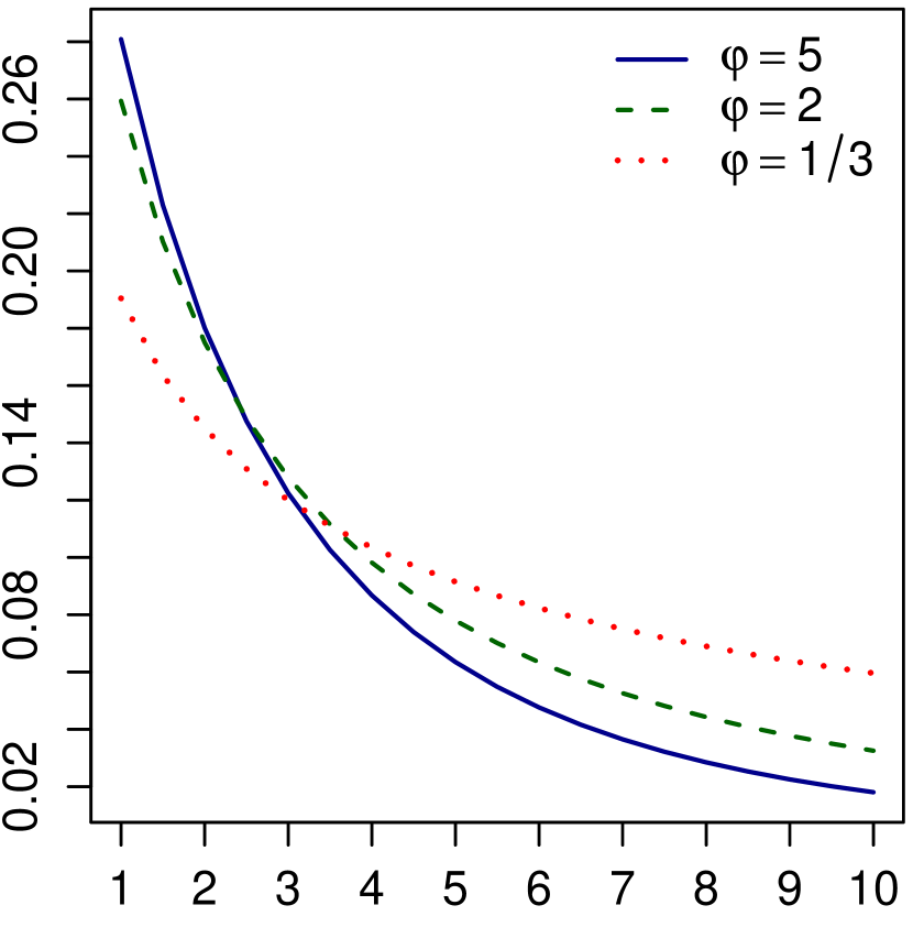
i IG$(1,\varphi)$

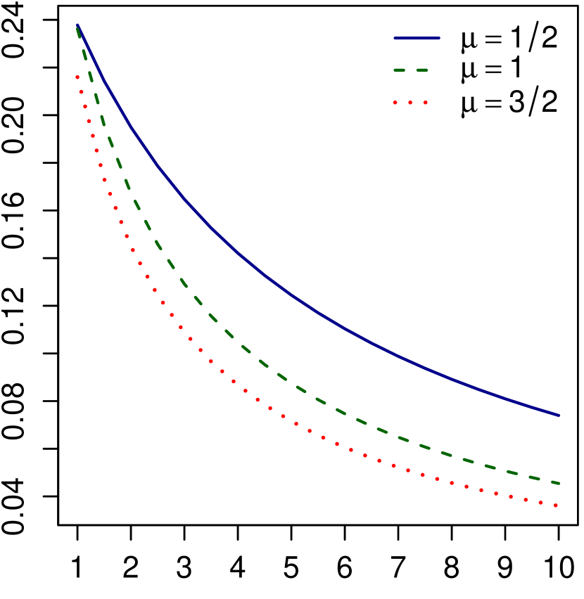
ii IG$(\mu,1)$

Figure 1. The tail probability $P(S>u)$ for different values of $\mu$ and $\varphi$.

Note that this particular selection for $\rho_{2}(\varTheta)$ and $P_{\varTheta}$ has also been adopted in a regression context by Tzougas et al. (2019);

(b) Analogously, if $\rho_{2}(\varTheta)=e^{-\varTheta}$, $v(\varTheta)=\varTheta^{3}$, then condition (10) becomes

$$P(S>u)=\mathbb{E}_{P}\Big{[}\big{(}1-e^{-\varTheta}\big{)}\cdot e^{-e^{-\varTheta}\cdot\varTheta^{3}\cdot u}\Big{]}\quad\text{for any }u>0.$$

Figure 2 depicts the tail probability $P(S>u)$ in the case $P_{\varTheta}=\textbf{Ga}(\alpha,\beta)$, where $\alpha,\beta>0$.

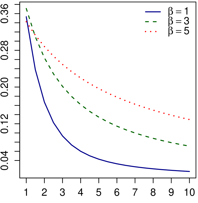
i Ga$(3,\beta)$

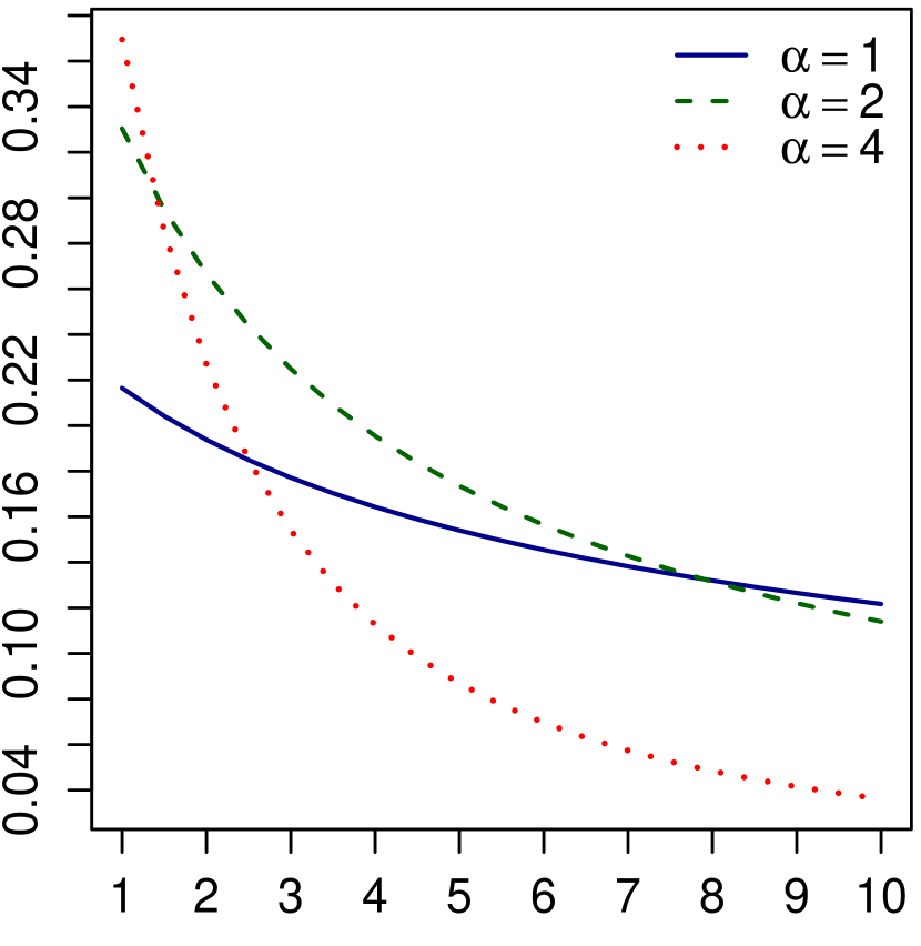
ii Ga$(\alpha,3)$

Figure 2. The tail probability $P(S>u)$ for different values of $\alpha$ and $\beta$.

Note that a similar mixture for $N$ has been studied by Gençtürk & Yiğiter (2016);

(c) Now, let $D=(0,1)$, $\rho_{2}(\varTheta)=\varTheta$ and $v(\varTheta)=-\ln\varTheta^{2}$. In this case, condition (10) can be rewritten as

$$P(S>u)=\mathbb{E}_{P}\Big{[}\big{(}1-\varTheta\big{)}\cdot\varTheta^{2\cdot u\cdot\varTheta}\Big{]}\quad\text{for any }u>0.$$

Figure 3 illustrates the tail probability $P(S>u)$ in the case $P_{\varTheta}=\textbf{Be}(\alpha,\beta)$, where $\alpha,\beta>0$. Note that such a mixture for $N$ has been considered by Wang (2011).

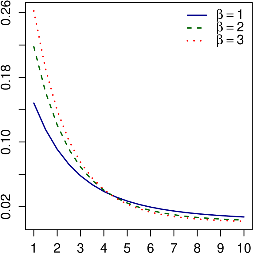
i Be$(3,\beta)$

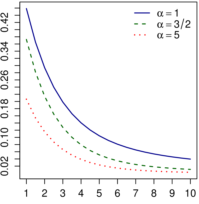
ii Be$(\alpha,3)$

Figure 3. The tail probability $P(S>u)$ for different values of $\alpha$ and $\beta$.

4. Recursive formulas for mixed compound distributions

Throughout what follows in this section, unless stated otherwise, $P_{S}={\bf MC}\big{(}P_{N},P_{X_{1}}\big{)}$ with $P_{N}\in\text{\bf Panjer}(a(\varTheta),b(\varTheta);0)$ and $P_{X_{1}}({\mathbb{N}}_{0})=1$.

Since in the collective risk model the random variable $S$ represents the total claim amount paid out from an insurance company over a fixed period of time, the determination of its pmf is of great importance. However, even in the classical case where $X$ is $P$-i.i.d. and $N,X$ are $P$-mutually independent, it is difficult to obtain a closed form for the pmf of $S$, which usually involves the computation of higher-order convolutions, a task that may be proven difficult, or at least time consuming. As a consequence, actuaries usually resort to recursive expressions, which seem to be more convenient and computationally efficient.

In the next result, we obtain a recursive formula for the pmf of $S$ by extending the famous Panjer recursion (cf., e.g., Schmidt (2012), Theorem 5.4.2) to the class $\text{\bf Panjer}(a(\varTheta),b(\varTheta);0)$. In order to present it, we denote by $m_{N\mid\varTheta}$ the conditional probability generating functions of $N$, i.e., $m_{N\mid\varTheta}(t)=\mathbb{E}_{P}\big{[}t^{N}\mid\varTheta\big{]}$ for any $t$ with $|t|\leq 1$.

Theorem 4.1.

There exists a family $\{\rho_{x}\}_{x\in{R}_{S}}$ of probability measures on $\varSigma$ defined by

$$\rho_{x}(A):=\frac{\mathbb{E}_{P}[\mathbbm{1}_{A}\cdot\mathbbm{1}_{\{S=x\}}]}{\mathbb{E}_{P}[\mathbbm{1}_{\{S=x\}}]}\quad\text{for any }A\in\varSigma$$

being an rcp of $P$ over $P_{S}$ consistent with $S$, such that

$$g(x)=\begin{cases}\mathbb{E}_{P}\big{[}m_{N\mid\varTheta}\big{(}f_{X_{1}\mid\varTheta}(0)\big{)}\big{]}&\text{, if }x=0\\ \sum_{y=1}^{x}D_{x,y}\cdot g(x-y)&\text{, if }x\in R_{S}\setminus\{0\}\end{cases},$$

where

$$D_{x,y}:=\mathbb{E}_{\rho_{x-y}}\bigg{[}\Big{(}a(\varTheta)+\frac{b(\varTheta)\cdot y}{x}\Big{)}\cdot\frac{f_{X_{1}\mid\varTheta}(y)}{1-a(\varTheta)\cdot f_{X_{1}\mid\varTheta}(0)}\bigg{]}$$

for any $x\in R_{S}\setminus\{0\}$ and $y\in\{1,\ldots,x\}$.

In particular, if $f_{X_{1}\mid\varTheta}(0)=0$ $P{\upharpoonright}\sigma(\varTheta)$-a.s. then

$$g(x)=\begin{cases}p_{0}&\text{, if }x=0\\ \sum_{y=1}^{x}D_{x,y}\cdot g(x-y)&\text{, if }x\in R_{S}\setminus\{0\}\end{cases},$$

where

$$D_{x,y}=\mathbb{E}_{\rho_{x-y}}\Big{[}\Big{(}a(\varTheta)+\frac{b(\varTheta)\cdot y}{x}\Big{)}\cdot\ f_{X_{1}\mid\varTheta}(y)\Big{]}$$

for any $x\in R_{S}\setminus\{0\}$ and $y\in\{1,\ldots,x\}$.

Proof.

Fix on arbitrary $x\in R_{S}$ and define the set-function $\rho_{x}:\varSigma\to(0,\infty)$ by

$$\rho_{x}(A):=\frac{\mathbb{E}_{P}[\mathbbm{1}_{A}\cdot\mathbbm{1}_{\{S=x\}}]}{\mathbb{E}_{P}[\mathbbm{1}_{\{S=x\}}]}\quad\text{for any }A\in\varSigma.$$

By applying similar arguments to those appearing in the proof of Theorem 2.11, it follows easily that the family $\{\rho_{y}\}_{y\in{R}_{S}}$ is an rcp of $P$ over $P_{S}$ consistent with $S$. Furthermore, first note that condition $g(0)=\mathbb{E}_{P}\big{[}m_{N\mid\varTheta}\big{(}f_{X_{1}\mid\varTheta}(0)\big{)}\big{]}$ is an immediate consequence of Corollary 3.7 for $B=\{0\}$. By Lyberopoulos & Macheras (2022), Lemmas 3.4(ii) and 3.3, the sequence $X$ is $P_{\theta}$-i.i.d. and $(N,X)$ are $P_{\theta}$-mutually independent for $P_{\varTheta}$-a.a. $\theta\in D$, respectively. Since $P_{N}\in{\bf Panjer}(a(\varTheta),b(\varTheta);0)$, Proposition 2.7 implies that $(P_{\theta})_{N}\in{\bf Panjer}(a(\theta),b(\theta);0)$ for $P_{\varTheta}$-a.a. $\theta\in D$; hence we may apply Schmidt (2012), Theorem 5.4.2, to get

$$g_{\theta}(x)=\frac{1}{1-a(\theta)\cdot f_{\theta}(0)}\cdot\sum_{y=1}^{x}\Big{(}a(\theta)+\frac{b(\theta)\cdot y}{x}\Big{)}\cdot f_{\theta}(y)\cdot g_{\theta}(x-y),$$

where $g_{\theta}$ denotes the pmf of $S$ with respect to $P_{\theta}$. The latter, together with Corollary 3.7 and Lemma 2.5, yields

$$g(x)=\sum_{y=1}^{x}\mathbb{E}_{P}\Big{[}\Big{(}a(\varTheta)+\frac{b(\varTheta)\cdot y}{x}\Big{)}\cdot\frac{f_{X_{1}\mid\varTheta}(y)}{1-a(\varTheta)\cdot f_{X_{1}\mid\varTheta}(0)}\cdot g_{\varTheta}(x-y)\Big{]}.$$ (11)

But since

$$\mathbb{E}_{\rho_{x}}[\mathbbm{1}_{\varTheta^{-1}[F]}]=\frac{\mathbb{E}_{P}[\mathbbm{1}_{\varTheta^{-1}[F]}\cdot\mathbbm{1}_{\{S=x\}}]}{\mathbb{E}_{P}[\mathbbm{1}_{\{S=x\}}]}=\frac{\mathbb{E}_{P_{\varTheta}}[\mathbbm{1}_{F}\cdot g_{\theta}(x)]}{g(x)}\quad\text{for each }F\in{\mathfrak{B}}(D),$$

where the second equality follows by Lemma 2.5, we easily get that

$$\begin{split}&\mathbb{E}_{P}\Big{[}\Big{(}a(\varTheta)+\frac{b(\varTheta)\cdot y}{x}\Big{)}\cdot\frac{f_{X_{1}\mid\varTheta}(y)}{1-a(\varTheta)\cdot f_{X_{1}\mid\varTheta}(0)}\cdot g_{\varTheta}(x-y)\Big{]}\\ &\quad=\mathbb{E}_{\rho_{x-y}}\Big{[}\Big{(}a(\varTheta)+\frac{b(\varTheta)\cdot y}{x}\Big{)}\cdot\frac{f_{X_{1}\mid\varTheta}(y)}{1-a(\varTheta)\cdot f_{X_{1}\mid\varTheta}(0)}\Big{]}\cdot g(x-y)\end{split}$$ (12)

for any $y\in\{1,\ldots,x\}$. Conditions (11) and (12) complete the first part of the proof.

In particular, first note that if $f_{X_{1}\mid\varTheta}(0)=0$ $P{\upharpoonright}\sigma(\varTheta)$-a.s., then $m_{N\mid\varTheta}\big{(}f_{X_{1}\mid\varTheta}(0)\big{)}=p_{0}(\varTheta)$ $P{\upharpoonright}\sigma(\varTheta)$-a.s.. The latter, along with conditions (11) and (12), completes the proof. ∎

Remark 4.2.

Assume that $P_{X_{1}}$ is absolutely continuous with respect to the Lebesgue measure $\lambda$ on ${\mathfrak{B}}(0,\infty)$. By applying the characterization appearing on Proposition 3.6 in conjunction with Panjer (1981), Theorem on p. 24, we can easily prove the equality

$$g(x)=\mathbb{E}_{P}\big{[}p_{1}(\varTheta)\cdot f_{X_{1}\mid\varTheta}(x)\big{]}+\int_{0}^{x}\mathbb{E}_{P}\bigg{[}\Big{(}\alpha(\varTheta)+\frac{b(\varTheta)\cdot y}{x}\Big{)}\cdot f_{X_{1}\mid\varTheta}(y)\cdot g_{\varTheta}(x-y)\bigg{]}\,\lambda(dy)$$ (13)

for any $x>0$. The integral equation (13) has to be solved numerically, however its implementation presents some serious difficulties (see Gómez-Déniz et al. (2004), p. 42). The proof of a recursion for $g$ in the spirit of Theorem 4.1 and its implementation is the subject of a forthcoming paper.

Remark 4.3.

If $X$ and $\varTheta$ are $P$-independent, it follows by Lemma 2.5 that $P_{X_{1}\mid\varTheta}=P_{X_{1}}$ $P{\upharpoonright}\sigma(\varTheta)$-a.s.. Hence Theorem 4.1 gives

$$g(x)=\begin{cases}\mathbb{E}_{P}\Big{[}m_{N\mid\varTheta}\big{(}f_{X_{1}}(0)\big{)}\Big{]}&\text{, if }x=0\\ \sum_{y=1}^{x}{D}_{x,y}\cdot g(x-y)&\text{, if }x\in R_{S}\setminus\{0\}\end{cases},$$

where ${D}_{x,y}=\mathbb{E}_{\rho_{x-y}}\Big{[}\frac{x\cdot a(\varTheta)+y\cdot b(\varTheta)}{x\cdot(1-a(\varTheta)\cdot f_{X_{1}}(0))}\Big{]}\cdot f_{X_{1}}(y)$ for any $x\in R_{S}\setminus\{0\}$ and $y\in\{1,\ldots,x\}$.

Recall that a sequence $Z:=\{Z_{n}\}_{n\in{\mathbb{N}}}$ of random variables on $\varOmega$ is called exchangeable, if the joint distribution of the sequence is invariant under the permutation of the indices (cf., e.g., Fremlin (2013), 459C). In non-classical Risk Theory, the concept of exchangeability seems to be an appealing way to introduce a dependence structure between the claim sizes. Actually, exchangeability can be a natural assumption in the risk model context (see Albrecher et al. (2011), Remark 2.7). Note that by Lyberopoulos & Macheras (2022), Proposition 4.1, we get that a sequence $Z$ is exchangeable under $P$ if and only if there exists a random vector $\widetilde{\varTheta}$ such that $Z$ is $P$-conditionally i.i.d. over $\sigma(\widetilde{\varTheta})$.

Corollary 4.4.

Let $\{\rho_{x}\}_{x\in{R}_{S}}$ be the family of probability measures constructed in Theorem 4.1. If $P_{N}\in{\bf Panjer}(a,b;0)$ and $N$, $\varTheta$ are $P$-independent then

$$g(x)=\begin{cases}\mathbb{E}_{P}\Big{[}m_{N}\big{(}f_{X_{1}\mid\varTheta}(0)\big{)}\Big{]}&\text{, if }x=0\\ \sum_{y=1}^{x}D_{x,y}\cdot g(x-y)&\text{, if }x\in R_{S}\setminus\{0\}\end{cases},$$

where $D_{x,y}=\big{(}a+b\cdot\frac{y}{x}\big{)}\cdot\mathbb{E}_{\rho_{x-y}}\Big{[}\frac{f_{X_{1}\mid\varTheta}(y)}{1-a\cdot f_{X_{1}\mid\varTheta}(0)}\Big{]}$ for any $x\in R_{S}\setminus\{0\}$ and $y\in\{1,\ldots,x\}$.

The proof follows immediately by Theorem 4.1 and therefore it is omitted.

The following example shows that if $P_{N}\in{\bf Panjer}(a(\varTheta),b(\varTheta);0)$, then the claim number distribution, for example in the case of an Excess of Loss reinsurance, remains in the same class, but with different parameters (cf., e.g., Schmidt (2012), p. 108).

Example 4.5.

Let $h$ be a ${\mathfrak{B}}(D)$-${\mathfrak{B}}(0,\infty)$-measurable function and set $v(\theta):=P_{\theta}(X_{1}>h(\theta))\in(0,1)$ for any $\theta\in D$. Fix an arbitrary $n\in{\mathbb{N}}$ and define the function $z_{n}:\varOmega\times D\rightarrow\{0,1\}$ by $z_{n}(\omega,\theta):=\mathbbm{1}_{\{X_{n}>h(\theta)\}}(\omega)$ for any $(\omega,\theta)\in\varOmega\times D$. For an arbitrary, but fixed $\theta\in D$, set $z(\theta):=\{z_{k}(\theta)\}_{k\in{\mathbb{N}}}$. Define the real-valued function $Z_{n}(\varTheta)$ on $\varOmega$ by $Z_{n}(\varTheta):=z_{n}\circ(id_{\varOmega}\times\varTheta)$ and the sequence $Z(\varTheta):=\{Z_{k}(\varTheta)\}_{k\in{\mathbb{N}}}$. Clearly $Z(\varTheta)$ is $P$-conditionally i.i.d. and $P$-conditionally independent of $N$ with $P_{Z_{n}(\varTheta)}={\bf MB}(1,v(\varTheta))$. Consider the random sum $M:=\sum_{k=1}^{N}Z_{k}(\varTheta)$. It then follows by Theorem 4.1 that

$$g(x)=\begin{cases}\mathbb{E}_{P}\big{[}m_{N\mid\varTheta}\big{(}1-v(\varTheta)\big{)}\big{]}&\text{, if }x=0\\ D_{x,1}\cdot g(x-1)&\text{, if }x\in R_{M}\setminus\{0\}\end{cases},$$

where

$$D_{x,1}=\mathbb{E}_{\rho_{x-1}}\bigg{[}\Big{(}\frac{a(\varTheta)\cdot v(\theta)}{1-a(\varTheta)\cdot\big{(}1-v(\varTheta)\big{)}}+\frac{1}{x}\cdot\frac{b(\varTheta)\cdot v(\varTheta)}{1-a(\varTheta)\cdot\big{(}1-v(\varTheta)\big{)}}\Big{)}\bigg{]}.$$

The latter, along with the fact that $P_{M}$ is a claim number distribution (cf., e.g., Schmidt (2012), Theorem 5.1.4), implies that $P_{M}\in{\bf Panjer}(\widetilde{a}(\varTheta),\widetilde{b}(\varTheta);0)$, where $\widetilde{a}(\varTheta):=\frac{a(\varTheta)\cdot v(\varTheta)}{1-a(\varTheta)\cdot\big{(}1-v(\varTheta)\big{)}}$ and $\widetilde{b}(\varTheta):=\frac{b(\varTheta)\cdot v(\varTheta)}{1-a(\varTheta)\cdot\big{(}1-v(\varTheta)\big{)}}$.

The following numerical examples demonstrate the behaviour of the pmf of the aggregate claims $S$. For illustrative purposes, we focus on three widely used mixing distributions in actuarial literature, namely the Inverse Gaussian (IG), the the Gamma (Ga) and the Beta (Be) distribution.

Example 4.6.

Let $D\subseteq(0,\infty)$ and $P_{N}=\textbf{MP}\big{(}\xi(\varTheta)\big{)}$, where $\xi$ is a ${\mathfrak{B}}(D)$-${\mathfrak{B}}(0,\infty)$-measurable function. Since $P_{N}\in{\bf Panjer}(a(\varTheta),b(\varTheta);0)$, we get $\alpha(\varTheta)=0$ and $b(\varTheta)=\xi(\varTheta)$ (see Table 1). Let $v$ be a ${\mathfrak{B}}(D)$-${\mathfrak{B}}(0,1)$-measurable function.

(a) Take $P_{X_{1}}=\textbf{MNB}\big{(}1,v(\varTheta)\big{)}$. Since $P_{X_{1}}({\mathbb{N}}_{0})=1$, we may apply Theorem 4.1 to get

$$g(x)=\begin{cases}\mathbb{E}_{P}\big{[}e^{\xi(\varTheta)\cdot(v(\varTheta)-1)}\big{]}&\text{, if }x=0\\ \sum_{y=1}^{x}D_{x,y}\cdot g(x-y)&\text{, if }x\in{\mathbb{N}}\end{cases},$$

where $D_{x,y}=\frac{y}{x}\cdot\mathbb{E}_{\rho_{x-y}}\Big{[}\xi(\varTheta)\cdot v(\varTheta)\cdot\big{(}1-v(\varTheta)\big{)}^{y}\Big{]}$ for any $x\in{\mathbb{N}}$ and $y\in\{1,\ldots,x\}$. Figure 4 depicts the behaviour of $g$ for $\xi(\varTheta)=\varTheta$ and $v(\varTheta)=\frac{\varTheta}{1+\varTheta}$.

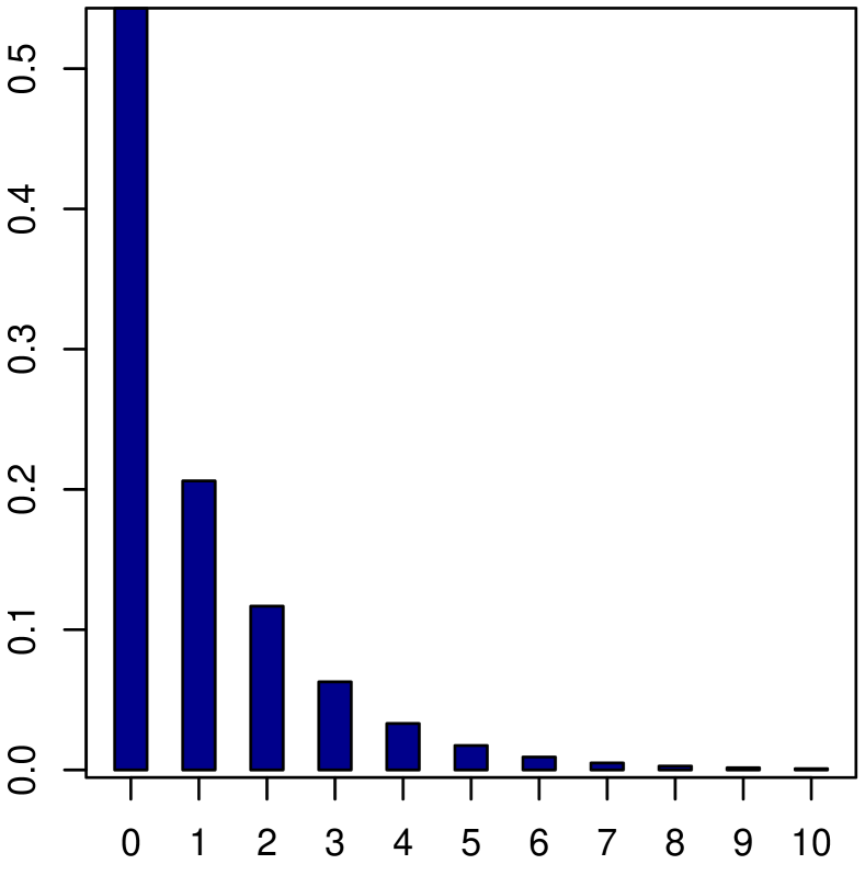
i IG$(2,5)$

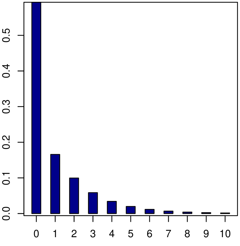
ii Ga$(5,4)$

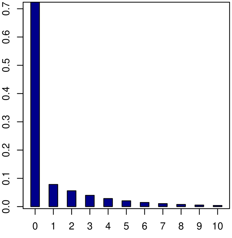
iii Be$(5,5)$

Figure 4. The pmf of $S$ for $P_{N}=\textbf{MP}(\varTheta)$ and $P_{X_{1}}=\textbf{MNB}\big{(}1,\frac{\varTheta}{1+\varTheta}\big{)}$.

(b) Assume now that the claim sizes are distributed according to a mixed zero truncated geometric distribution with parameter $v(\varTheta)$ (written $\textbf{MZTG}\big{(}v(\varTheta)\big{)}$ for short), i.e.,

$$f_{X_{1}\mid\varTheta}(x)=v(\varTheta)\cdot\big{(}1-v(\varTheta)\big{)}^{x-1}\quad P{\upharpoonright}\sigma(\varTheta)\text{-a.s.}$$

for any $x\in{\mathbb{N}}$. Since $P_{X_{1}}({\mathbb{N}}_{0})=1$ with $f_{X_{1}\mid\varTheta}(0)=0$ $P{\upharpoonright}\sigma(\varTheta)$-a.s., we may apply Theorem 4.1 to get

$$g(x)=\begin{cases}\mathbb{E}_{P}\big{[}e^{-\xi(\varTheta)}\big{]}&\text{, if }x=0\\ \sum_{y=1}^{x}D_{x,y}\cdot g(x-y)&\text{, if }x\in{\mathbb{N}}\end{cases},$$

where $D_{x,y}=\frac{y}{x}\cdot\mathbb{E}_{\rho_{x-y}}\big{[}\xi(\varTheta)\cdot v(\varTheta)\cdot\big{(}1-v(\varTheta)\big{)}^{y-1}\big{]}$ for any $x\in{\mathbb{N}}$ and $y\in\{1,\ldots,x\}$. Figure 5 illustrates the behaviour of $g$ for the same choices of $\xi(\varTheta)$ and $v(\varTheta)$ as in (a).

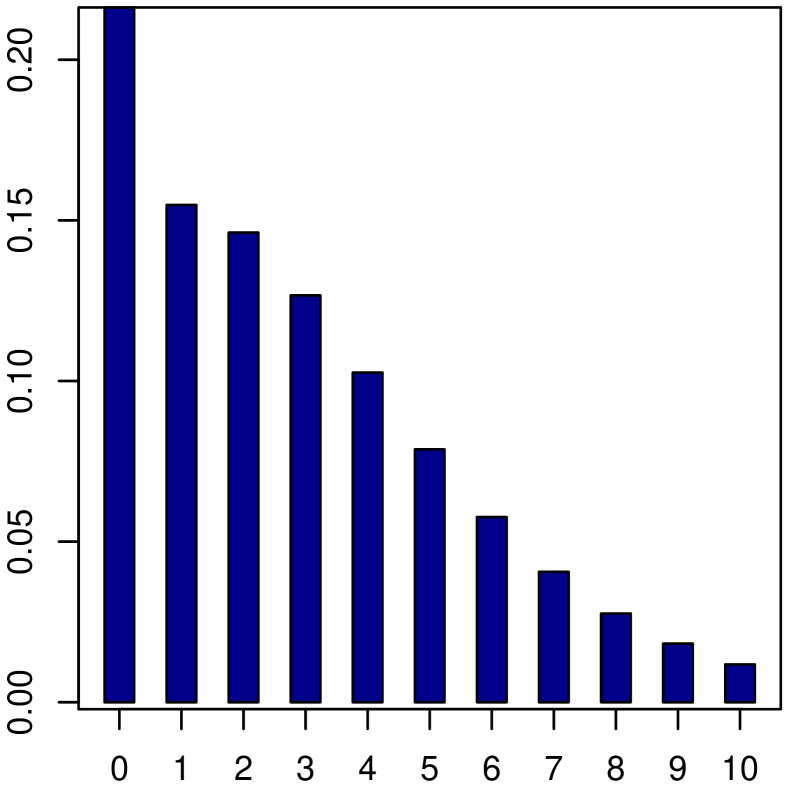
i IG$(2,5)$

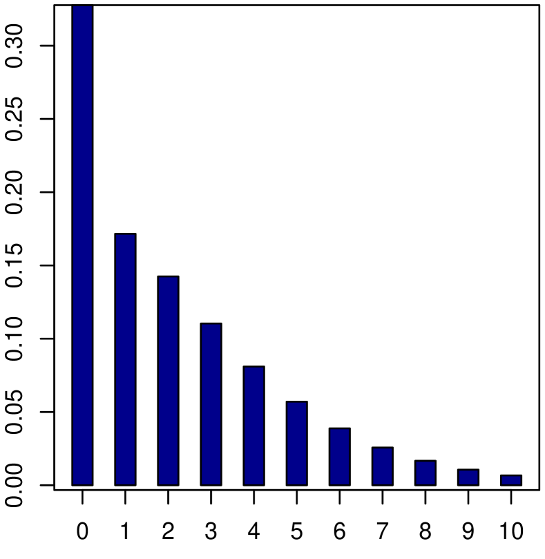
ii Ga$(5,4)$

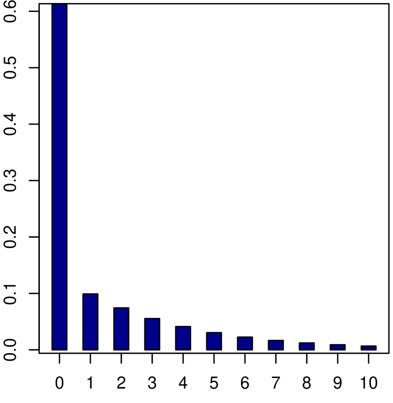
iii Be$(5,5)$

Figure 5. The pmf of $S$ for $P_{N}=\textbf{MP}(\varTheta)$ and $P_{X_{1}}=\textbf{MZTG}\big{(}\frac{\varTheta}{1+\varTheta}\big{)}$.

(c) Assume that $X$ and $\varTheta$ are $P$-independent and that $v(\varTheta)$ is degenerate at some point $p\in(0,1)$. If $P_{X_{1}}=\textbf{ZTG}(p)$, then we can apply Theorem 4.1, along with Remark 4.3(a), to get

$$g(x)=\begin{cases}\mathbb{E}_{P}\big{[}e^{-\xi(\varTheta)}\big{]}&\text{, if }x=0\\ \sum_{y=1}^{x}{D}_{x,y}\cdot g(x-y)&\text{, if }x\in{\mathbb{N}}\end{cases},$$

where ${D}_{x,y}=\frac{y}{x}\cdot p\cdot(1-p)^{y-1}\cdot\mathbb{E}_{\rho_{x-y}}\big{[}\xi(\varTheta)\big{]}$ for any $x\in{\mathbb{N}}$ and $y\in\{1,\ldots,x\}$. Figure 6 depicts $g$ for $p=3/5$ and $\xi(\varTheta)$ as in (a).

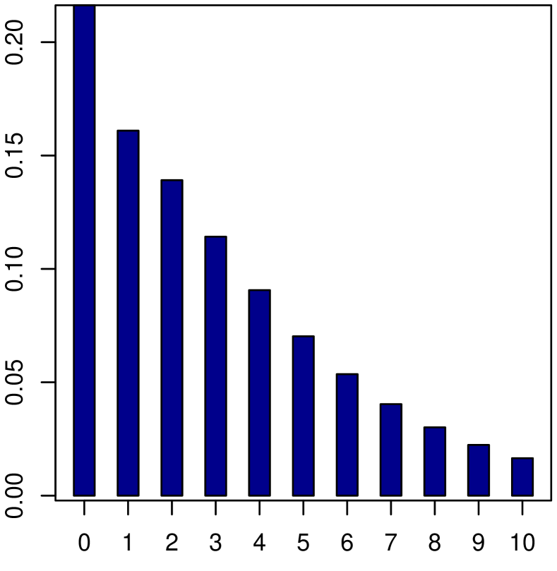
i IG$(2,5)$

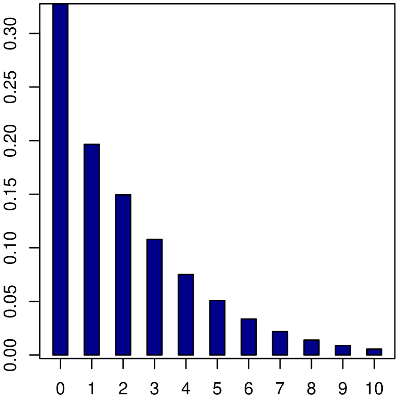
ii Ga$(5,4)$

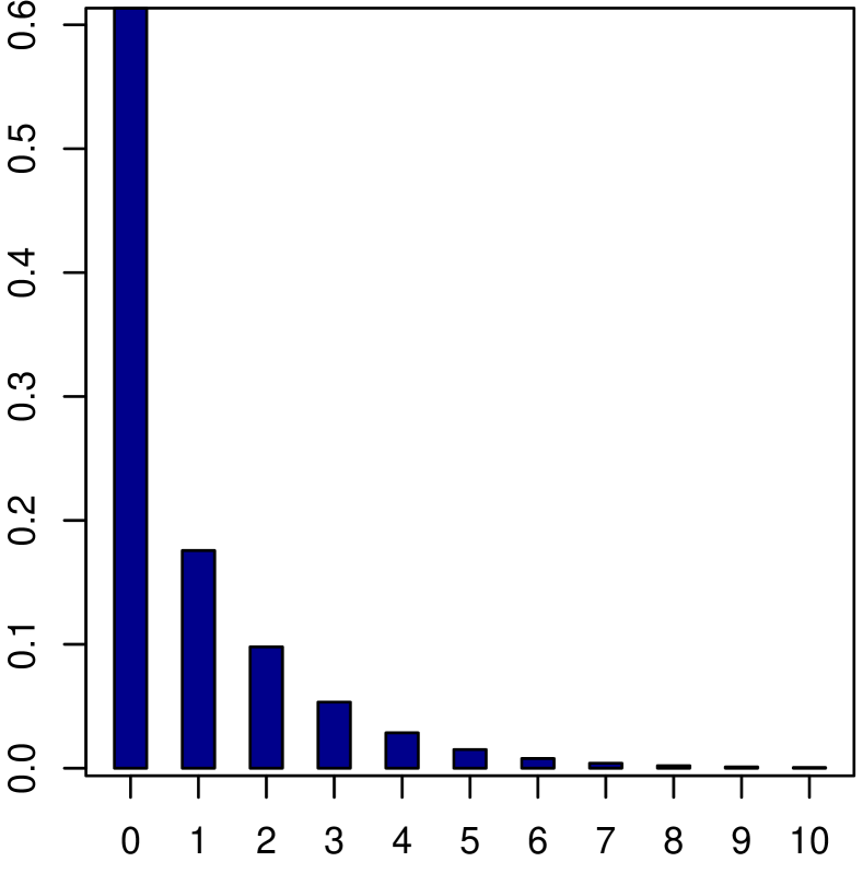
iii Be$(5,5)$

Figure 6. The pmf of $S$ for $P_{N}=\textbf{MP}(\varTheta)$ and $P_{X_{1}}=\textbf{ZTG}\big{(}\frac{3}{5}\big{)}$.

(d) Assume that $N$ and $\varTheta$ are $P$-independent and that $\xi(\varTheta)$ is degenerate at some point $\theta_{0}\in D$. If $P_{X_{1}}=\textbf{MZTG}\big{(}v(\varTheta)\big{)}$, we may apply Corollary 4.4 to get

$$g(x)=\begin{cases}e^{-\theta_{0}}&\text{, if }x=0\\ \sum_{y=1}^{x}{D}_{x,y}\cdot g(x-y)&\text{, if }x\in{\mathbb{N}}\end{cases},$$

where ${D}_{x,y}=\frac{y\cdot\theta_{0}}{x}\cdot\mathbb{E}_{\rho_{x-y}}\big{[}v(\varTheta)\cdot\big{(}1-v(\varTheta)\big{)}^{y-1}\big{]}$ for any $x\in{\mathbb{N}}$ and $y\in\{1,\ldots x\}$. Figure 7 exhibits $g$ for $\theta_{0}=3$ and $v(\varTheta)$ as in (a).

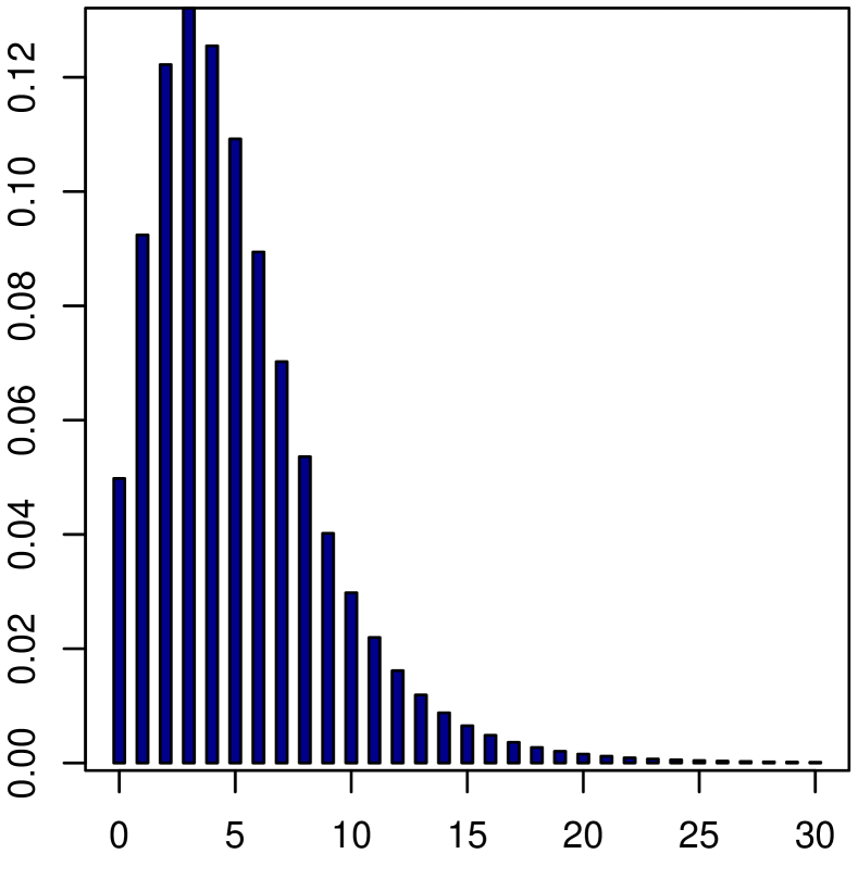
i IG$(2,5)$

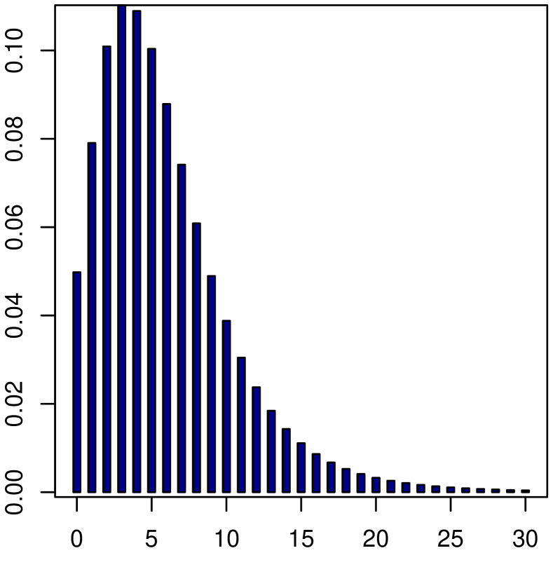
ii Ga$(5,4)$

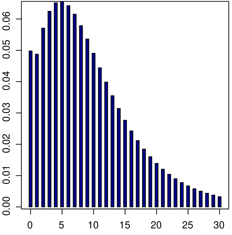
iii Be$(5,5)$

Figure 7. The pmf of $S$ for $P_{N}=\textbf{P}(3)$ and $P_{X_{1}}=\textbf{MZTG}\big{(}\frac{\varTheta}{1+\varTheta}\big{)}$.

Example 4.7.

Let $D\subseteq(0,\infty)$, $P_{N}=\textbf{MNB}\big{(}\rho_{1}(\varTheta),\rho_{2}(\varTheta)\big{)}$, where $\rho_{1},\rho_{2}$ are ${\mathfrak{B}}(D)$-${\mathfrak{B}}(0,\infty)$- and ${\mathfrak{B}}(D)$-${\mathfrak{B}}(0,1)$-measurable functions, respectively. Since $P_{N}\in{\bf Panjer}(a(\varTheta),b(\varTheta);0)$, we get $\alpha(\varTheta)=1-\rho_{2}(\varTheta)$ and $b(\varTheta)=\big{(}\rho_{1}(\varTheta)-1\big{)}\cdot\big{(}1-\rho_{2}(\varTheta)\big{)}$ (see Table 1). Take $P_{X_{1}}=\textbf{MZTG}\big{(}\frac{\varTheta}{1+\varTheta}\big{)}$.

(a) Let $\big{(}\rho_{1}(\theta),\rho_{2}(\theta)\big{)}=\big{(}\theta,e^{-\theta}\big{)}$ for any $\theta\in D$. Since $\alpha(\varTheta)=1-e^{-\varTheta}$ and $b(\varTheta)=(\varTheta-1)\cdot\big{(}1-e^{-\varTheta}\big{)}$, we may apply Theorem 4.1 to get

$$g(x)=\begin{cases}\mathbb{E}_{P}\big{[}e^{-\varTheta^{2}}\big{]}&\text{, if }x=0\\ \sum_{y=1}^{x}D_{x,y}\cdot g(x-y)&\text{, if }x\in{\mathbb{N}}\end{cases},$$

where $D_{x,y}=\mathbb{E}_{\rho_{x-y}}\Big{[}\big{(}1+(\varTheta-1)\cdot\frac{y}{x}\big{)}\cdot\frac{(1-e^{-\varTheta})\cdot\varTheta}{(1+\varTheta)^{y}}\Big{]}$ for any $x\in{\mathbb{N}}$ and $y\in\{1,\ldots,x\}$ (see Figure 8).

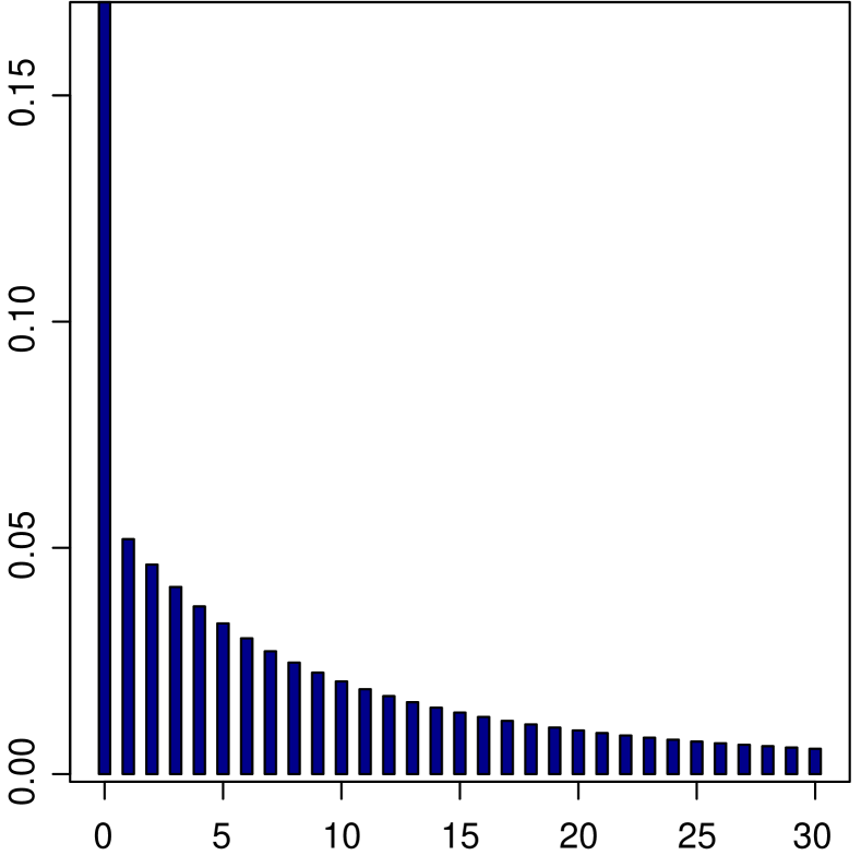
i IG$(2,5)$

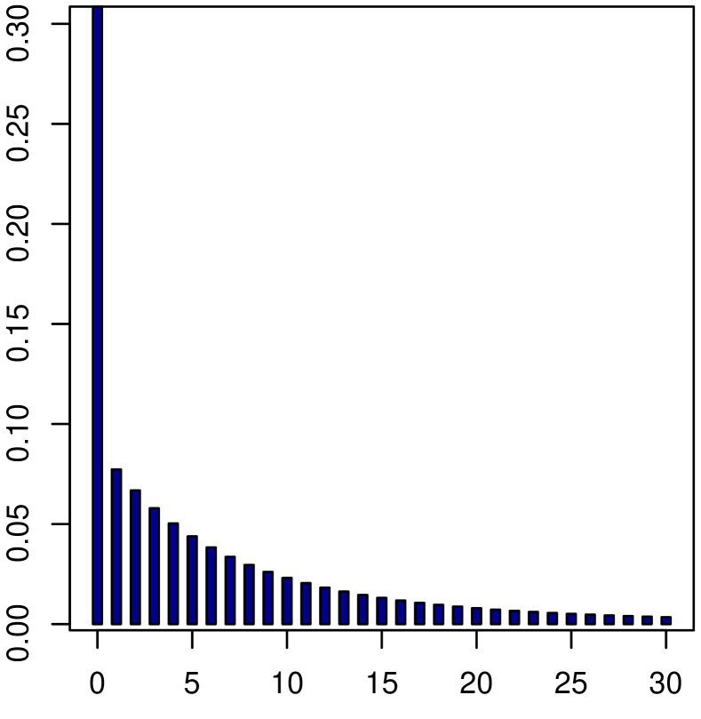
ii Ga$(5,4)$

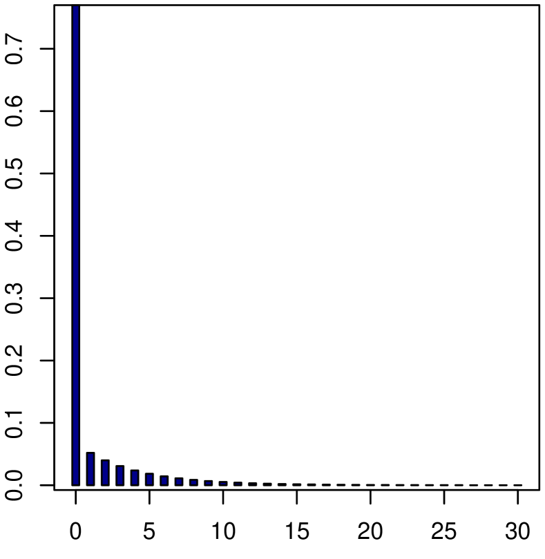
iii Be$(5,5)$

Figure 8. The pmf of $S$ for $P_{N}=\textbf{MNB}\big{(}\varTheta,e^{-\varTheta}\big{)}$ and $P_{X_{1}}=\textbf{MZTG}\big{(}\frac{\varTheta}{1+\varTheta}\big{)}$.

(b) Now take $\big{(}\rho_{1}(\theta),\rho_{2}(\theta)\big{)}=\big{(}2\theta,\frac{1}{1+\theta}\big{)}$ for any $\theta\in D$. As $\alpha(\varTheta)=\frac{\varTheta}{1+\varTheta}$ and $b(\varTheta)=(2\varTheta-1)\cdot\frac{\varTheta}{1+\varTheta}$, we can apply Theorem 4.1 to obtain

$$g(x)=\begin{cases}\mathbb{E}_{P}\Big{[}\big{(}\frac{1}{1+\varTheta}\big{)}^{2\varTheta}\Big{]}&\text{, if }x=0\\ \sum_{y=1}^{x}D_{x,y}\cdot g(x-y)&\text{, if }x\in{\mathbb{N}}\end{cases},$$

where $D_{x,y}=\mathbb{E}_{\rho_{x-y}}\Big{[}\big{(}1+(2\varTheta-1)\cdot\frac{y}{x}\big{)}\cdot\frac{\varTheta^{2}}{(1+\varTheta)^{y+1}}\Big{]}$ for any $x\in{\mathbb{N}}$ and $y\in\{1,\ldots,x\}$ (see Figure 9).

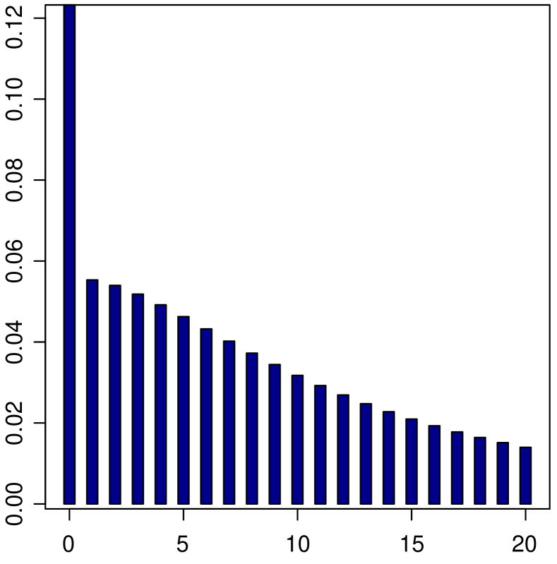
i IG$(2,5)$

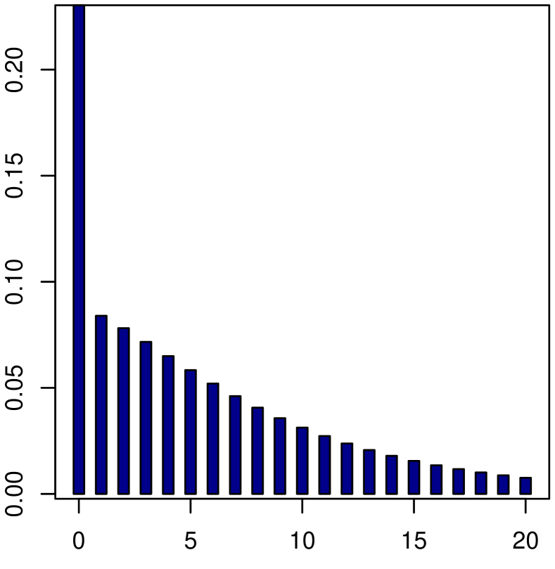
ii Ga$(5,4)$

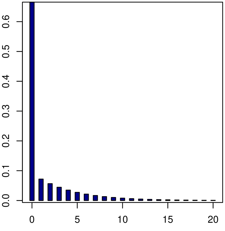
iii Be$(5,5)$

Figure 9. The pmf of $S$ with $P_{N}=\textbf{MNB}\big{(}2\varTheta,\frac{1}{1+\varTheta}\big{)}$ and $P_{X_{1}}=\textbf{MZTG}\big{(}\frac{\varTheta}{1+\varTheta}\big{)}$.

(c) Let $D=(0,1)$ and take $\big{(}\rho_{1}(\theta),\rho_{2}(\theta)\big{)}=(r,\theta)$ for any $\theta\in D$, where $r>0$. Since $\alpha(\varTheta)=1-\varTheta$ and $b(\varTheta)=(r-1)\cdot(1-\varTheta)$, we can apply Theorem 4.1 to obtain

$$g(x)=\begin{cases}\mathbb{E}_{P}\big{[}\varTheta^{r}\big{]}&\text{, if }x=0\\ \sum_{y=1}^{x}D_{x,y}\cdot g(x-y)&\text{, if }x\in{\mathbb{N}}\end{cases},$$

where $D_{x,y}=\big{(}1+(r-1)\cdot\frac{y}{x}\big{)}\cdot\mathbb{E}_{\rho_{x-y}}\Big{[}\frac{(1-\varTheta)\cdot\varTheta}{(1+\varTheta)^{y}}\Big{]}$ for any $x\in{\mathbb{N}}$ and $y\in\{1,\ldots,x\}$. Figure 10 illustrates $g$ for $P_{\varTheta}=\textbf{Be}(\alpha,\beta)$, where $\alpha,\beta>0$, and different values of $r$.

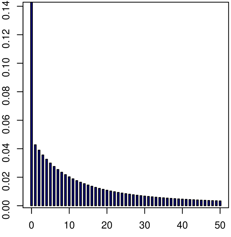
i $r=2$; $\alpha=2$; $\beta=4$

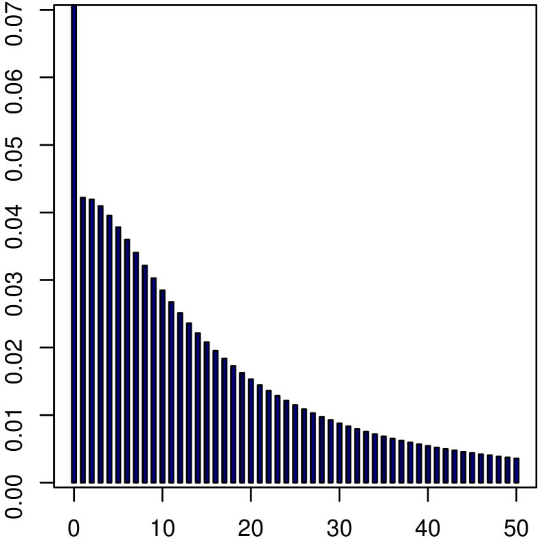
ii $r=5$; $\alpha=4$; $\beta=4$

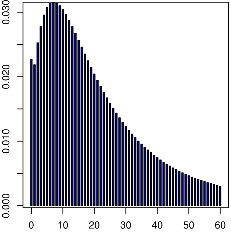
iii $r=10$; $\alpha=7$; $\beta=5$

Figure 10. The pmf of $S$ for different values of $r$, $\alpha$ and $\beta$.

(d) Let $D=(0,\infty)$ and take $\big{(}\rho_{1}(\theta),\rho_{2}(\theta)\big{)}=(\theta,p)$ for any $\theta\in D$, where $p\in(0,1)$. As $\alpha(\varTheta)=1-p$ and $b(\varTheta)=(\varTheta-1)\cdot(1-p)$, we can apply Theorem 4.1 to obtain

$$g(x)=\begin{cases}\mathbb{E}_{P}\big{[}p^{\varTheta}\big{]}&\text{, if }x=0\\ \sum_{y=1}^{x}D_{x,y}\cdot g(x-y)&\text{, if }x\in{\mathbb{N}}\end{cases},$$

where $D_{x,y}=(1-p)\cdot\mathbb{E}_{\rho_{x-y}}\Big{[}\big{(}1+(\varTheta-1)\cdot\frac{y}{x}\big{)}\cdot\frac{\varTheta}{(1+\varTheta)^{y}}\Big{]}$ for any $x\in{\mathbb{N}}$ and $y\in\{1,\ldots,x\}$. Figure 11 depicts $g$ for $P_{\varTheta}=\textbf{Ga}(\alpha,\beta)$, where $\alpha,\beta>0$, and various values of $p$.

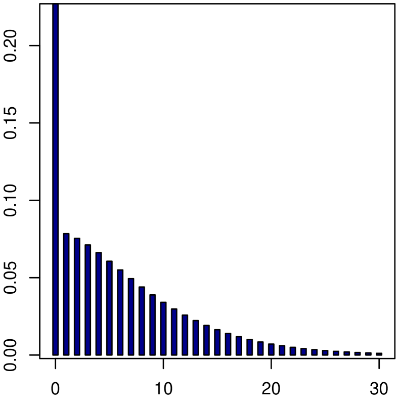
i $p=1/3$; $\alpha=2$; $\beta=1$

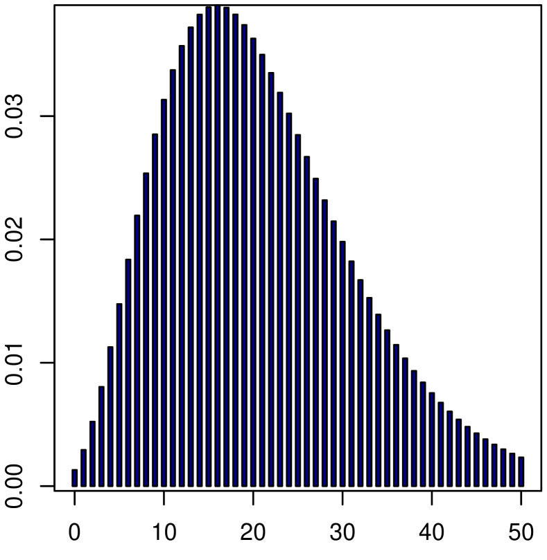
ii $p=1/2$; $\alpha=5$; $\beta=1/4$

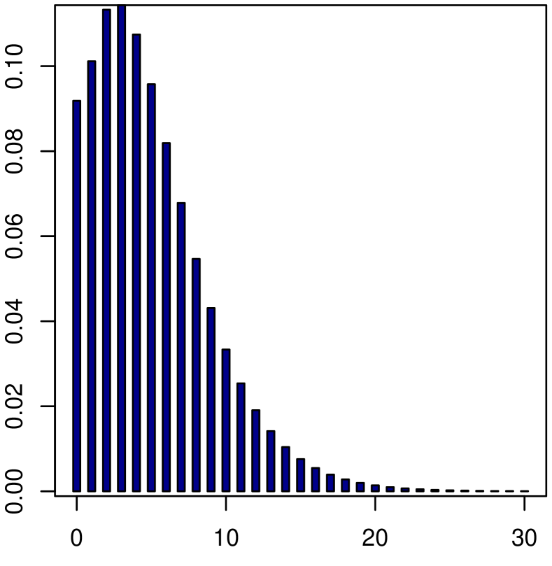
iii $p=2/3$; $\alpha=3$; $\beta=1/3$

Figure 11. The pmf of $S$ for different values of $p$, $\alpha$ and $\beta$.

(e) Assume that $N$ and $\varTheta$ are $P$-independent and let $\big{(}\rho_{1}(\theta),\rho_{2}(\theta)\big{)}=(r,p)$ for any $\theta\in D$, where $r>0$ and $p\in(0,1)$. Since $\alpha=1-p$ and $b=(r-1)\cdot(1-p)$, we can apply Corollary 4.4 to obtain

$$g(x)=\begin{cases}p^{r}&\text{, if }x=0\\ \sum_{y=1}^{x}D_{x,y}(F)\cdot g(x-y)&\text{, if }x\in{\mathbb{N}}\end{cases},$$

where $D_{x,y}=(1-p)\cdot\big{(}1+(r-1)\cdot\frac{y}{x}\big{)}\cdot\mathbb{E}_{\rho_{x-y}}\Big{[}\frac{\varTheta}{(1+\varTheta)^{y}}\Big{]}$ for any $x\in{\mathbb{N}}$ and $y\in\{1,\ldots,x\}$ (see Figure 12).

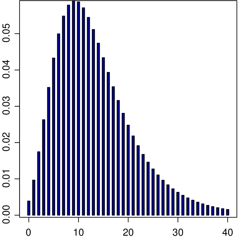
i IG$(2,5)$

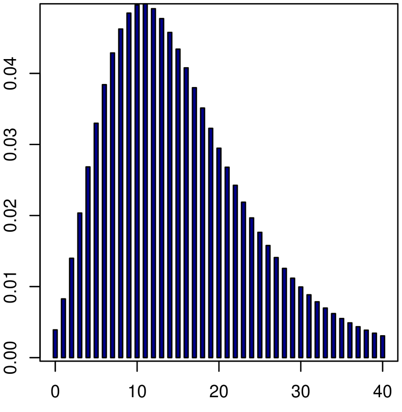
ii Ga$(5,4)$

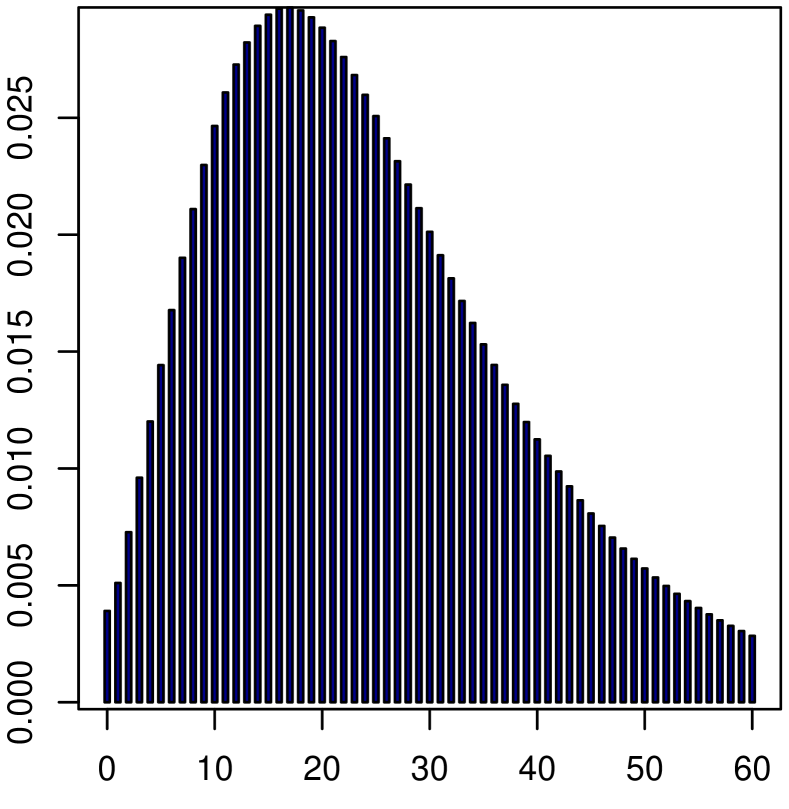
iii Be$(5,5)$

Figure 12. The pmf of $S$ with $P_{N}=\textbf{NB}(8,1/2)$ and $P_{X_{1}}=\textbf{MZTG}\big{(}\frac{\varTheta}{1+\varTheta}\big{)}$.

Example 4.8.

Let $D\subseteq(0,\infty)$, $P_{N}=\textbf{MB}\big{(}n,z_{2}(\varTheta)\big{)}$, where $n\in{\mathbb{N}}$ and $z_{2}$ is a ${\mathfrak{B}}(D)$-${\mathfrak{B}}(0,1)$-measurable function. As $P_{N}\in{\bf Panjer}(a(\varTheta),b(\varTheta);0)$, we get $\alpha(\varTheta)=-\frac{z_{2}(\varTheta)}{1-z_{2}(\varTheta)}$ and $b(\varTheta)=(n+1)\cdot\frac{z_{2}(\varTheta)}{1-z_{2}(\varTheta)}$ (see Table 1). Take $P_{X_{1}}=\textbf{MZTG}\big{(}\frac{\varTheta}{1+\varTheta}\big{)}$.

(a) Let $D=(0,1)$ and take $z_{2}(\theta)=1-\theta$ for any $\theta\in D$. Since $\alpha(\varTheta)=-\frac{1-\varTheta}{\varTheta}$ and $b(\varTheta)=(n+1)\cdot\frac{1-\varTheta}{\varTheta}$, we may apply Theorem 4.1 to get

$$g(x)=\begin{cases}\mathbb{E}_{P}\big{[}\varTheta^{n}\big{]}&\text{, if }x=0\\ \sum_{y=1}^{x}D_{x,y}\cdot g(x-y)&\text{, if }x\in{\mathbb{N}}\end{cases},$$

where $D_{x,y}=\big{(}-1+(n+1)\cdot\frac{y}{x}\big{)}\cdot\mathbb{E}_{\rho_{x-y}}\big{[}\frac{1-\varTheta}{(1+\varTheta)^{y}}\big{]}$ for any $x\in{\mathbb{N}}$ and $y\in\{1,\ldots,x\}$. Figure 13 depicts $g$ for $P_{\varTheta}=\textbf{Be}(\alpha,\beta)$, where $\alpha,\beta>0$, and different values of $n$.

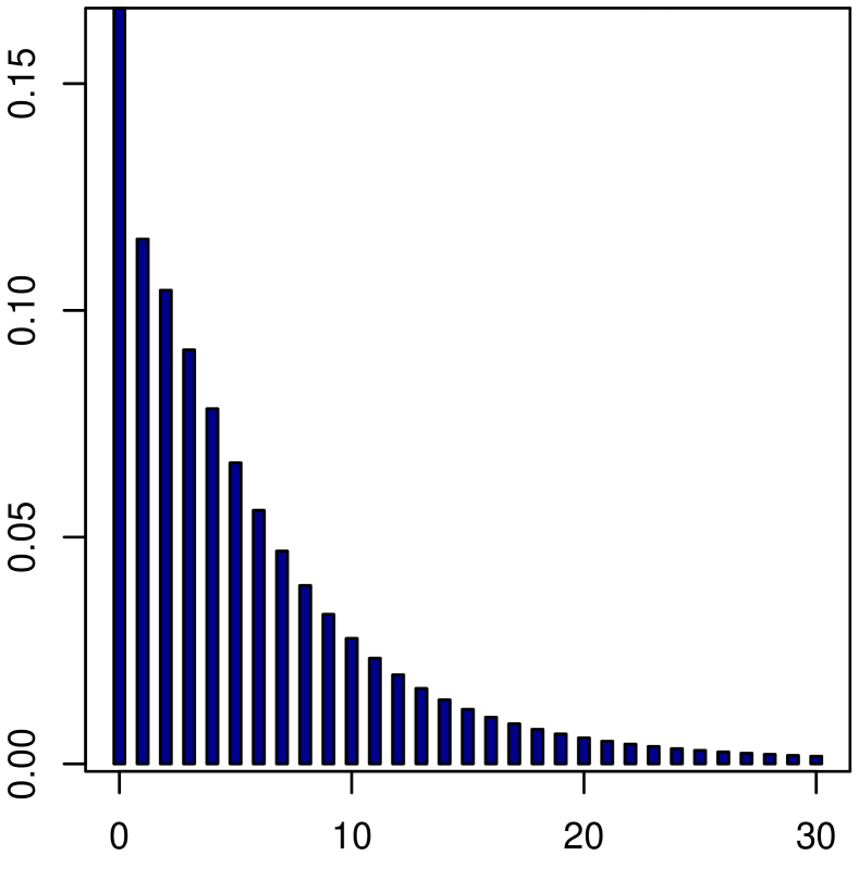
i $n=2$; $\alpha=3$; $\beta=5$

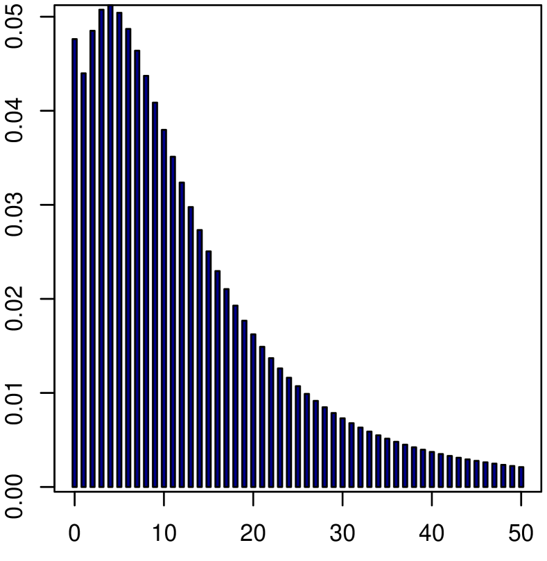
ii $n=5$; $\alpha=2$; $\beta=3$

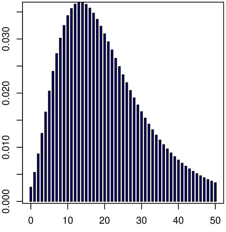
iii $n=10$; $\alpha=6$; $\beta=8$

Figure 13. The pmf of $S$ for different values of $n$, $\alpha$ and $\beta$.

(b) Let $D=(0,\infty)$ and take $z_{2}(\theta)=e^{-\theta}$ for any $\theta\in D$. As $\alpha(\varTheta)=-\frac{e^{-\varTheta}}{1-e^{-\varTheta}}$ and $b(\varTheta)=(n+1)\cdot\frac{e^{-\varTheta}}{1-e^{-\varTheta}}$, we may apply Theorem 4.1, together with Remark 4.3(a), to get

$$g(x)=\begin{cases}\mathbb{E}_{P}\Big{[}\big{(}1-e^{-\varTheta}\big{)}^{n}\Big{]}&\text{, if }x=0\\ \sum_{y=1}^{x}D_{x,y}\cdot g(x-y)&\text{, if }x\in{\mathbb{N}}\end{cases},$$

where $D_{x,y}=\big{(}-1+(n+1)\cdot\frac{y}{x}\big{)}\cdot\mathbb{E}_{\rho_{x-y}}\Big{[}\frac{\varTheta\cdot e^{-\varTheta}}{(1-e^{-\varTheta})\cdot(1+\varTheta)^{y}}\Big{]}$ for any $x\in{\mathbb{N}}$ and $y\in\{1,\ldots,x\}$. Figure 14 illustrates $g$ for $P_{\varTheta}=\textbf{Ga}(\alpha,\beta)$, where $\alpha,\beta>0$, and various values of $n$.

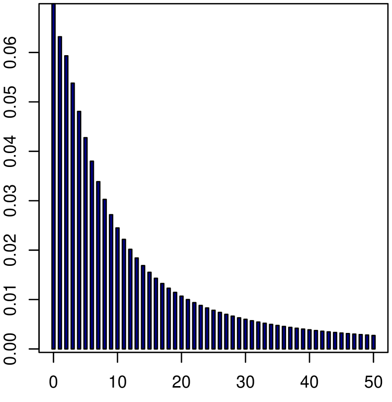
i $n=2$; $\alpha=3/4$; $\beta=3$

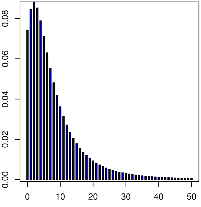
ii $n=5$; $\alpha=3$; $\beta=4$

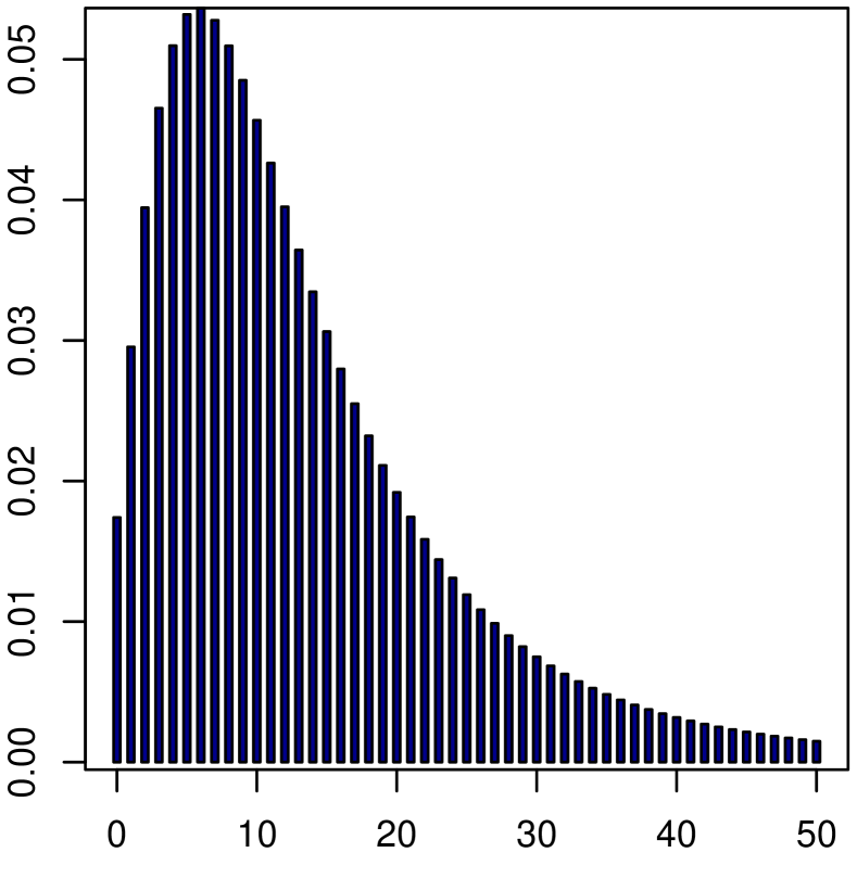
iii $n=10$; $\alpha=4$; $\beta=5$

Figure 14. The pmf of $S$ for different values of $n$, $\alpha$ and $\beta$.

(c) Let $D=(0,\infty)$ and take $z_{2}(\theta)=\frac{1}{1+\theta}$ for any $\theta\in D$. Since $\alpha(\varTheta)=-\frac{1}{\varTheta}$ and $b(\varTheta)=\frac{(n+1)}{\varTheta}$, we may apply Theorem 4.1 to get

$$g(x)=\begin{cases}\mathbb{E}_{P}\Big{[}\big{(}\frac{\varTheta}{1+\varTheta}\big{)}^{n}\Big{]}&\text{, if }x=0\\ \sum_{y=1}^{x}D_{x,y}\cdot g(x-y)&\text{, if }x\in{\mathbb{N}}\end{cases},$$

where $D_{x,y}=\big{(}-1+(n+1)\cdot\frac{y}{x}\big{)}\cdot\mathbb{E}_{\rho_{x-y}}\Big{[}\frac{1}{(1+\varTheta)^{y}}\Big{]}$ for any $x\in{\mathbb{N}}$ and $y\in\{1,\ldots,x\}$. Figure 15 depicts $g$ for $P_{\varTheta}=\textbf{IG}(\mu,\varphi)$, where $\mu,\varphi>0$, and different values of $n$.

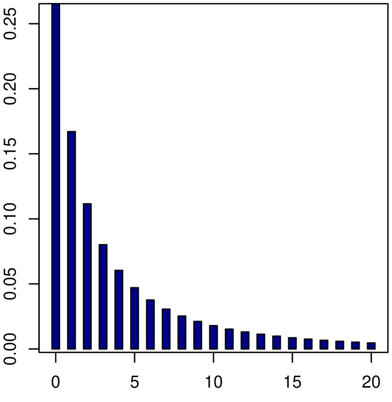
i $n=2$; $\mu=2$; $\varphi=1/2$

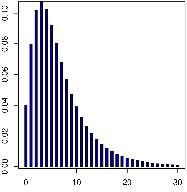
ii $n=5$; $\mu=1$; $\varphi=3$

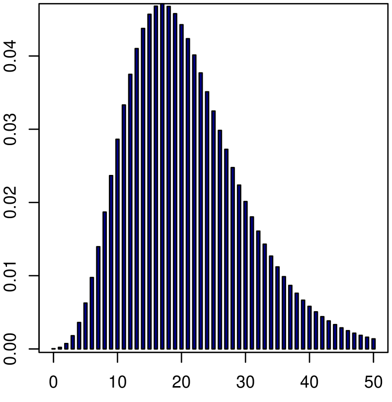
iii $n=10$; $\mu=0.5$; $\varphi=10$

Figure 15. The pmf of $S$ for different values of $n$, $\mu$ and $\varphi$.

5. Concluding Remarks

When dealing with inhomogeneous insurance portfolios, mixtures of claim number distributions are frequently used to model the claim counts. In actuarial practice, the usual independence assumptions seem to be unrealistic. In particular, the mutual independence between claims sizes and counts appears to be implausible, especially when considering inhomogeneous portfolios. The above led us to the development of this work.

This paper aims to investigate the mixed counterpart of the original ${\bf Panjer}(a,b;0)$ class and the corresponding compound distributions by relaxing the usual independence assumptions in two ways. More specifically, we allow the parameters of the claim number and the claim size distributions to be random, and we assume that the claim size process is conditionally i.i.d. and conditionally mutually independent of the claim counts.

Based on the above assumptions and the fundamental concept of regular conditional probabilities, this work provides a characterization for the members of ${\bf Panjer}(a(\varTheta),b(\varTheta);0)$ class, as well as two recursive algorithms for $P_{N}$ and $P_{S}$, respectively, where the recursion for $P_{S}$ also covers the case of a compound Panjer distribution with exchangeable claims. Our results are accompanied by various numerical examples to highlight the practical relevance of this work.

It is worth mentioning that the members of the ${\bf Panjer}(a(\varTheta),b(\varTheta);0)$ class may be of particular interest in non-life insurance problems, for example, when insurance data exhibit overdispersion. Finally, this research allows us to consider some possible extensions of actuarial interest beyond the scopes of this paper, such as the study of the mixed counterpart of ${\bf Panjer}(a,b;k)$ for $k\geq 1$ and the derivation of De Pril’s recursion for the moments of $S$ (see De Pril (1986), Theorem, p. 118).

References

Albrecher & Boxma (2004)Albrecher, H. & Boxma, O. J. (2004). A ruin model with dependence between claim sizes and claim intervals. Insurance: Mathematics and Economics, 35(2), 245–254.
Albrecher & Teugels (2006)Albrecher, H. & Teugels, J. L. (2006). Exponential behavior in the presence of dependence in risk theory. Journal of Applied Probability, 43(1), 257–273.
Albrecher et al. (2011)Albrecher, H., Constantinescu, C. & Loisel, S. (2011). Explicit ruin formulas for models with dependence among risks. Insurance: Mathematics and Economics, 48(2), 265–270.
Antzoulakos & Chadjiconstantinidis (2004)Antzoulakos, D. L. & Chadjiconstantinidis, S. (2004). On mixed and compound mixed Poisson distributions. Scandinavian Actuarial Journal, 2004(3), 161–188.
Beal (1940)Beal, G. (1940). The fit and significance of contagious distributions when applied to observations on larval insects. Ecology, 21(4), 460–474.
Chang & Pollard (1997)Chang, J. T. & Pollard, D. (1997). Conditioning as disintegration. Statistica Neerlandica, 51(3), 287–317.
Cohn (2013)Cohn, D. L. (2013). Measure Theory, 2nd ed. Birkhäuser Advanced Texts.
De Pril (1986)De Pril, N. (1986). Moments of a class of compound distributions . Scandinavian Actuarial Journal, 1986(2), 117–120.
Fackler (2023)Fackler M. (2023). Panjer class revisited: one formula for the distributions of the Panjer class. Annals of Actuarial Science, 17(1), 145–169.
Faden (1985)Faden, A. M. (1985). The existence of regular conditional probabilities: Necessary and sufficient conditions. Annals of Probability, 13(1), 288–298.
Fremlin (2013)Fremlin, D. H. (2013). Measure theory (Vol. 4). Torres Fremlin (Ed.).
Gençtürk & Yiğiter (2016)Gençtürk, Y. & Yiğiter, A. (2016). Modelling claim number using a new mixture model: negative binomial gamma distribution. Journal of Statistical Computation and Simulation, 86(10), 1829–1839.
Gerhold et al. (2010)Gerhold, S., Schmock, U. & Warnung, R. (2010). A generalization of Panjer’s recursion and numerically stable risk aggregation. Finance and Stochastics, 14(1), 81–128.
Ghitany et al. (2008)Ghitany, M. E., Atieh, B. & Nadarajah, S. (2008). Lindley distribution and its application. Mathematics and computers in simulation, 78(4), 493–506.
Gómez-Déniz et al. (2004)Gómez-Déniz, E., Sarabia, J. M. & Calderín-Ojeda, E. (2008). Univariate and multivariate versions of the negative binomial-inverse Gaussian distributions with applications. Insurance: Mathematics and Economics, 42(1), 39–49.
Grandell (1997)Grandell, J. (1997). Mixed Poisson Processes, Chapman & Hall.
Johnson et al. (2005)Johnson, N. L., Kotz, S. & Kemp, A. W. (2005). Univariate Discrete Distributions, 3rd ed. John Wiley and Sons, New York.
Hess et al. (2002)Hess, K. T., Liewald, A. & Schmidt, K. D. (2002) An extension of Panjer’s recursion. ASTIN Bulletin: The Journal of the IAA, 32(2), 61–80.
Hesselager (1994)Hesselager, O. (1994). A recursive procedure for calculation of some compound distributions. ASTIN Bulletin: The Journal of the IAA, 24(1), 19–32.
Hesselager (1996)Hesselager, O. (1996). A recursive procedure for calculation of some mixed compound Poisson distributions. Scandinavian Actuarial Journal1996(1), 54–63.
Karlis & Xekalaki (2005)Karlis, D. & Xekalaki, E. (2005). Mixed poisson distributions. International Statistical Review/Revue Internationale de Statistique, 73(1), 35–58.
Kolev & Paiva (2008)Kolev, N. & Paiva, D. (2008). Random sums of exchangeable variables and actuarial applications. Insurance: Mathematics and Economics, 42(1), 147–153.