Compositional Models for Estimating Causal Effects

Abstract

Many real-world systems can be represented as sets of interacting components. Examples of such systems include computational systems such as query processors, natural systems such as cells, and social systems such as families. Many approaches have been proposed in traditional (associational) machine learning to model such structured systems, including statistical relational models and graph neural networks. Despite this prior work, existing approaches to estimating causal effects typically treat such systems as single units, represent them with a fixed set of variables, and assume a homogeneous data-generating process. We study a compositional approach for estimating individual treatment effects (ITE) in structured systems, where each unit is represented by the composition of multiple heterogeneous components. This approach uses a modular architecture to model potential outcomes for each component and aggregates component-level potential outcomes to obtain the unit-level potential outcomes. We discover novel benefits of the compositional approach in causal inference — systematic generalization to estimate counterfactual outcomes of unseen combinations of components and improved overlap guarantees between treatment and control groups compared to the classical methods for causal effect estimation. We also introduce a set of novel environments for empirically evaluating the compositional approach and demonstrate the effectiveness of our approach using simulated and real-world data.

1 Introduction

Causal inference is central to empirical research and scientific discovery. Inferring causal effects from observational data is an important problem in many fields of science, such as medicine, economics, and education [Morgan and Winship, 2015]. Many scientific and engineering challenges require understanding treatment effect heterogeneity, including personalized medicine [Curth et al., 2024] and custom online advertising [Bottou et al., 2013]. Existing approaches for causal effect estimation usually assume that each unit of study is represented by a fixed set of features sampled from the data-generating process that is homogeneous across all the units in the population, known as unit homogeneity assumption [Holland, 1986]. However, many real-world systems are modular, i.e., they decompose into heterogeneous functional components that interact to produce system behavior [Callebaut and Rasskin-Gutman, 2005, Johnson and Ahn, 2017]. Input data to such systems is often structured and of variable size, reflecting the underlying modular structure of the system. Examples of structured inputs processed by modular systems include DNA sequences processed by cells, computer programs processed by compilers, and natural language queries processed by language models. Estimating heterogeneous treatment effects on complex real-world variable-size structured inputs is an important problem, especially as the complexity of modern technological systems increases.

To provide a simple and concrete example of the type of causal inference problem that we focus on in this paper, consider the following example of an arithmetic computation system consisting of addition, subtraction, multiplication, and division modules (see Figure 1(a)). The system takes arithmetic expressions as input — e.g., $((1+2)*(5-3))+(10/5)$ — and returns the value of the expression as output (e.g., $8$). In this example, input expressions are structured units of a “compositional” nature, i.e., they comprise multiple component operations that can combine to generate new units in multiple ways. These kinds of inputs can be represented as hierarchical graphs, e.g., parse-trees, where each node is an operation and edges represent the information flow between the components. Given such a system, consider the task of modeling the causal effect of different memory sizes on the processing time of different arithmetic expressions. This problem can be formulated as estimating the individual-level effect. In the terminology of causal inference, each arithmetic expression is a unit of analysis, the features of the arithmetic expression are pre-treatment covariates, memory size is the intervention, and processing time is the potential outcome [Rubin, 1974, 2005].

The standard approaches to heterogeneous treatment effect estimation [Hill, 2011, Athey and Imbens, 2016, Wager and Athey, 2018, Chernozhukov et al., 2018] usually represent each unit using a fixed-size feature vector. For example, in the case of arithmetic expressions, we can use the number of operations in each unit and operand values as covariates and estimate the individual-level treatment effect by conditioning on these features. However, using fixed-size representation for compositional units such as the arithmetic expressions above poses several estimation challenges: (1) As the structure and complexity of each unit varies, estimating effects at the unit level requires reasoning about the similarity among the heterogeneous units in high-dimensional space; (2) Each unit has an instance-specific composition of the basic operations, representing all the units with the same features would lead to sparse feature representation and aggregation of the features of multiple occurrences of each operation; (3) The approach does not exploit the compositionality of the units and each new unit with an unseen combination of the component operations would require reasoning from scratch.

We propose a compositional approach to causal effect estimation for structured units represented as hierarchical graphs. This approach constructs an instance-specific causal model with a modular architecture representing the components for each unit and estimates the unit-level intervention’s effects at the component level. By exploiting fine-grained information about the structure of modular systems, such as execution traces in software programs, query plans in databases, and log data in monitoring systems, the compositional approach takes advantage of detailed information about the system’s structure and behavior, which often remain unused. The compositional approach decomposes causal queries into more fine-grained queries, focusing on how unit-level interventions affect component-level outcomes to produce the overall unit’s outcome. This framing offers benefits such as improved sample efficiency, better overlap between treatment and control groups, enhanced out-of-distribution effect estimation on units with unseen combinations of components, causal effect estimation for realistic interventions that involve adding, removing, or replacing modules in the system, and scalable causal effect estimation for variable-length units without facing the curse of dimensionality. These potential benefits make the compositional approach promising for causal effect estimation in complex, modular systems.

Despite these potential benefits, learning compositional models for effect estimation has pitfalls, including a larger number of parameters to estimate, sensitivity to errors in individual components, and errors in modeling component interactions. In this paper, we investigate the conditions under which the compositional approach provides benefits over standard approaches. Our findings indicate that compositional models provide better estimates of individual treatment effects as overlap issues increase and offer systematic generalization benefits on out-of-distribution units, particularly when the underlying system comprises multiple heterogeneous components. Specifically, we:

Formalize the compositional approach to causal effect estimation: We formalize causal effect estimation for structured units, outline possible types of compositions of potential outcomes in real-world examples, provide algorithms to learn compositional models for different composition types, and discuss the assumptions required to identify individual treatment effects from observational data using the compositional approach.

Analyze the theoretical benefits of compositional models: We use the generalization bounds for individual-level treatment effect estimation [Shalit et al., 2017] to decompose the compositional model’s generalization error into factual and counterfactual errors of the component models. We discuss the assumptions of better component-level overlap and the existence of heterogeneous components with independent mechanisms, under which compositionality leads to better estimation of factual and counterfactual errors, resulting in improved generalization performance.

Propose a set of real-world evaluation environments: We propose a set of novel real-world evaluation environments to evaluate the compositional approach, including query execution in relational databases for different memory sizes and matrix processing on different types of computer hardware. We evaluate the performance of the compositional approach compared to existing approaches on both synthetic and real-world data sets.

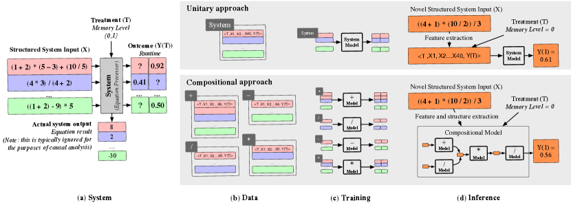
Figure 1: Overview of key ideas: (a) System: An example arithmetic system that takes structured expressions (units) as input, returns values as output. Runtime (potential outcome) is observed for each expression for a given memory level (treatment). (b) Data: Fixed-size data includes high-dimensional covariates and treatment for each unit. In contrast, compositional data consists of lower-dimensional component-specific covariates and treatment, possibly with multiple samples per unit. (c) Training: The "unitary approach" uses fixed-size data to estimate unit-level potential outcomes. The compositional model uses compositional data to estimate component-level potential outcomes, aggregating them to estimate unit-level outcomes. (d) Inference: For a novel unit (possibly with unseen component combinations), the compositional approach instantiates an instance-specific model with modular architecture similar to the interaction structure of the components.

Other real-world use cases for the compositional approach to reason about interventions’ effects and make informed, personalized decisions are detailed in the supplementary material (Section B).

2 Related Work

We briefly discuss the connections of the compositional approach with the existing work in causal inference and associational machine learning.

Causal inference in structured domains: In causal inference, a relatively sparse body of work has focused on treatment effect estimation on structured data in modular domains [Gelman and Hill, 2006, Salimi et al., 2020, Kaddour et al., 2021]. For example, existing work in multi-level modeling and hierarchical causal models [Gelman and Hill, 2006, Witty and Jensen, 2018, Weinstein and Blei, 2024] leverages hierarchical data structure to improve effect estimation under unobserved confounders. There is also growing interest in heterogeneous effect estimation for complex data, such as images [Jerzak et al., 2022], structured treatments (e.g., graphs, images, text, drugs) [Harada and Kashima, 2021, Kaddour et al., 2021], and relational data [Salimi et al., 2020, Khatami et al., 2024]. The compositional approach complements this line of research by providing fine-grained analysis of individual effect estimation on structured units and using modular architectures for variable-size compositional data, offering systematic generalization benefits for effect estimation tasks. Also, our focus lies in the structured and compositional representation of entire units rather than only treatments, which helps better estimate causal effects in the case of high-dimensional observational data. Other related work is in the fine-grained analysis of the potential outcomes to study the validity of synthetic control methods with panel data [Shi et al., 2022].

Compositional models in associational machine learning: Our work is inspired by research on compositional models in machine learning that exploit the structure of underlying domains and explicitly represent it in the model structure [Heckerman and Wellman, 1995, Koller and Pfeffer, 1997, Friedman et al., 1999, Getoor and Taskar, 2007, Taskar et al., 2005, Laskey, 2008]. The closest work to our proposed compositional models is the use of recursive neural networks [Socher et al., 2011] and modular neural networks [Andreas et al., 2016, Marcus and Papaemmanouil, 2019] in vision and language domains. However, most of the work in machine learning focuses on understanding the systematic generalization and sample efficiency benefits of compositional models for prediction tasks, while their role in reasoning about intervention effects is unexplored [Lake and Baroni, 2018, Hupkes et al., 2020, Wiedemer et al., 2024]. Our work addresses this gap.

3 Compositional Approach for Causal Effect Estimation

In this section, we introduce a compositional representation of structured units and potential outcomes and provide an algorithm to estimate individual treatment effects for the structured units from the observational data using compositional models.

Preliminaries: Let us assume that for a unit $i$ with pre-treatment covariates $X_{i}=x\in\mathcal{X}\subset\mathbb{R}^{d}$ and a binary treatment $T_{i}\in\{0,1\}$, there are two potential outcomes $\{Y_{i}(0),Y_{i}(1)\}\in\mathcal{Y}\subset\mathbb{R}$ [Rubin, 1974, 2005]. In the observational data, we only observe one of the potential outcomes for each unit, depending on the treatment assignment. We refer to $Y_{i}=Y_{i}(T_{i})$ as the observed/factual outcome and ${Y_{i}}_{CF}=Y_{i}(1-T_{i})$ as the unobserved/counterfactual outcome. Individual treatment effect (ITE) is defined as $\tau(x):\mathbb{E}[Y_{i}(1)-Y_{i}(0)|X_{i}=x]$. Estimating ITE requires assumptions of unconfoundedness, overlap, and consistency [Rosenbaum and Rubin, 1983]. Under these assumptions, $\tau(x)$ is identifiable by $\tau(x)=\mathbb{E}[{Y_{i}|X_{i}=x,t=1}]-\mathbb{E}[{Y_{i}|X_{i}=x,t=0}]$ [Pearl, 2009]. The general strategy to estimate ITE is to directly estimate the conditional expectations of the outcomes using a single model with treatment as a feature or by fitting two separate regression models [Künzel et al., 2019]. Other approaches include propensity score-based adjustments and doubly robust methods [Kennedy, 2023]. We illustrate the compositional approach by directly estimating the potential outcomes. We use the term “unitary models" to denote non-compositional approaches that don’t consider the underlying structure and use fixed-size representation.

Compositional representation of the units and potential outcomes: We adopt a system view to describe how the units of analysis can be decomposed and represented using a small set of basic components. Consider a modular system with $k$ heterogeneous components $\{C_{1},C_{2},\dots C_{k}\}$. The units share this set of reusable components (See Figure 1 for the system summary). Each structured input $Q_{i}$ to the system can be represented as a tuple $(G_{i},\{\mathbf{X}_{ij}\}_{j=1:m_{i}})$ where $G_{i}$ is a tree-like hierarchical graph representing the instance-specific interaction among components, $\mathbf{X}_{ij}\in\mathbb{R}^{d_{j}}$ are input features to the $j^{th}$ component and $m_{i}$ is the number of components involved. More specifically, the graph $G_{i}$ represents the order in which the $m_{i}$ components process the structured unit, which variables $\mathbf{X}_{ij}$ are passed as an input to each component and how variables are shared among the components. Note that $m_{i}$ can be greater than the number of distinct components $k$ in the system, indicating the presence of multiple instances of each component type to represent each data instance. The number and kind of components required to process each input are specific to each unit. As an alternative to the compositional representation, a structured unit can also be represented using a fixed-size representation in the form of a single high-dimensional feature vector, $\mathbf{X}_{i}\in\mathbb{R}^{d}$ that represents the aggregation of the component level input features $\{\mathbf{X}_{ij}\}_{j=1}^{m}$. For example, see Figure 1(b) for the example fixed-size and compositional data representation. An example of the aggregation function includes concatenating the input features of each component and adding the input features of multiple instances of each component. We assume that a treatment $T_{i}$ is selected for each unit, which can affect the potential outcomes of some or all components using different mechanisms. For instance, in an arithmetic system, memory size can affect the execution time of some or all operations using separate mechanisms. Although component-level treatments that only affect one type of component can also be selected, we restrict our focus to unit-level treatments in this work to compare the compositional approach with non-compositional (unitary) approaches. Let $Y_{i}(t)\in\mathbb{R}$ denote the unit-level potential outcome under treatment $t$ for a unit $Q_{i}$, and let $\{Y_{ij}(0),Y_{ij}(1)\}_{j=1:m_{i}}$ denote the fine-grained component-level potential outcomes.

Difference between system output and potential outcome: Note that the output of the system itself and the outcome we wish to estimate can be different. For example, in the arithmetic example, the result of the arithmetic expression is the system’s output, but the execution time of the expression is the potential outcome of interest. In practical applications of causal reasoning, it is often useful to understand the effects of interventions on system behavior, and such behavior is often represented by key performance indicators (e.g., latency, efficiency, cost, and accuracy [Li et al., 2010, Bottou et al., 2013]).

We aim to estimate ITE for structured units from observational data. Due to each unit’s varying structure and complexity, satisfying the overlap assumption at the unit level becomes challenging when using a high-dimensional $\mathbf{X}_{i}$ non-compositional representation of the units [D’Amour et al., 2021]. Instead, we exploit the underlying compositionality of the system by reasoning about the component-level potential outcomes $Y_{ij}(t)$ for comparatively lower-dimensional component-level features $\mathbf{X}_{ij}\in\mathbb{R}^{d_{j}}(d_{j}<d)$ as covariates and given unit-level intervention $T_{i}=t$. The lower-dimensional representation of the component-level features compared to the unit-level features is generally true for most systems, as not all the unit-level features are relevant to compute the outcome of each component.

Types of composition: Parallel, sequential, and hierarchical: The composition of component-level potential outcomes to generate the unit-level potential outcome depends on the specific outcome, intervention type, system characteristics, and interaction structure $G_{i}$ of the components. We categorize kinds of composition into parallel, sequential, and hierarchical, based on the dependence among component-level potential outcomes. Parallel composition assumes that the potential outcomes of each component can be computed independently of the potential outcomes of the other components because there is no direct interaction among the potential outcomes for the components. In the arithmetic example, this assumes that the processing time of one arithmetic operation under a memory level can be assumed to be conditionally independent of the processing times of the other operations, given the input features of that component and shared treatment. This composition is similar to spatial composition in vision and reinforcement learning [Higgins et al., 2017, Van Niekerk et al., 2019]. A special case is additive parallel composition, where the composition function is addition. Sequential composition assumes that the potential outcomes of components have chain-like causal dependencies, where a component’s potential outcome depends on the values of other components’ potential outcomes, similar to the chained composition of policies in reinforcement learning [Sutton et al., 1999]. Hierarchical composition assumes that some potential outcomes can be computed independently while others have sequential dependencies. We assume that the instance-specific interaction structure $G_{i}$ among the components defines the structure of the hierarchical composition and is known.

Composition models for individual treatment effect estimation: We briefly describe the model training and inference for two kinds of composition models — (1) parallel composition model and (2) hierarchical composition model. Detailed model description and algorithms for training and inference are provided in the supplementary material (Algorithms 1, 2, Algorithms 3, and 4). See Figure 1(c) and (d) for the general description of model training and inference for compositional models. The additive parallel composition model estimates ITE using fine-grained potential outcomes with independently trained component models $(\hat{f}_{\theta_{j}})$ . During inference, component-level potential outcomes are aggregated, assuming additive composition to estimate unit-level outcomes, encoding conditional independence of component-level outcomes given their causes. The hierarchical composition model accounts for direct effects among component potential outcomes, with component models trained jointly end-to-end based on the interaction structure $G_{i}$. Potential outcomes are computed in post-order traversal, and ITE is estimated using the last component’s outcome (see Figure 1 (d) for an example). When only unit-level outcomes are observed, a version of the hierarchical model can be trained, assuming access to only component-level features and the interaction graph. We demonstrate in our experiments that hierarchical models with unit-level outcomes achieve comparable performance to models with access to fine-grained outcomes.

4 Theoretical Analysis

Theorem 4.1.

The CATE estimand for a structured unit $Q_{i}=q$ in case of additive parallel composition is equal to the additive composition of the component-level CATE estimands and is identified by the following: $\tau(q)=\sum_{j=1}^{m_{i}}\mathbb{E}[y_{ij}|\mathbf{x}_{ij},t=1]-\mathbb{E}[y_{ij}|\mathbf{x_{ij}},t=0]$, if we assume that unconfoundedness (G), overlap (H) and consistency (I) holds at the component level.

The proof is provided in the supplementary material (D.1). The theorem implies that if effects are identified at the component level and can be computed independently, then unit-level effects can be estimated using the sum of component-level effects. This result allows us to decompose the compositional model’s error into the component model’s errors, as we demonstrate in the next section.

Decomposition of the generalization error of the additive parallel compositional model

The treatment effect estimate of additive model $\hat{f}_{add}$ for unit $q$ is $\hat{\tau}_{\hat{f}_{add}}(q)=\hat{f_{add}}(q,1)-\hat{f_{add}}(q,0)$. We use precision in the estimation of heterogeneous effect (PEHE) loss [Hill, 2011], which is defined by the mean squared error difference in the estimated effect and the ground truth effect: $\epsilon_{PEHE}(\hat{f})=\mathbb{E}[(\hat{\tau}_{\hat{f}}(q)-\tau(q))^{2}]$. Using the results of the Theorem 4.1, it can be easily shown that the error of the additive parallel compositional model can be decomposed into the sum of the errors of individual components and pair-wise covariance between the errors of the component models, similar to the generalization error analysis of the ensemble models [Ueda and Nakano, 1996]. This decomposition implies that if the data-generating process of the component potential functions is very similar, then the errors of the component models would be highly correlated, and errors would aggregate. The more heterogeneous the components are, the more benefits there are from the compositional approach.

$$\epsilon_{PEHE}(f_{add})=\sum_{j=1}^{m_{i}}{\epsilon_{PEHE}(\hat{f}_{\theta_{j}})}+\sum_{j}\sum_{k,k\neq j}\sqrt{{\epsilon_{PEHE}(\hat{f}_{\theta_{j}})}}\sqrt{{\epsilon_{PEHE}(\hat{f}_{\theta_{k}})}}$$ (1)

Decomposition of error into factual and counterfactual errors: The factual $(\epsilon_{F})$ and counterfactual errors $(\epsilon_{CF})$ are defined as : $\epsilon_{F}(\hat{f})=\mathbb{E}[(\hat{f}(q)-y)^{2}]$, $\epsilon_{CF}(\hat{f})=\mathbb{E}[\hat{f}(q,1-t)-y_{CF}]^{2}$. Similarly, factual and counterfactual errors for the treatment and control population are denoted as $\epsilon^{t=0}_{F}$, $\epsilon^{t=1}_{F}$, $\epsilon^{t=0}_{CF}$, and $\epsilon^{t=1}_{CF}$.

Previous work [Shalit et al., 2017] provides upper bounds for generalization error bounds for ITE estimators that decompose PEHE into the sum of factual and counterfactual errors. This work also shows that the counterfactual error can be upper bounded by the sum of factual error and distribution mismatch between treatment $P(X=x|T=0)$ and control populations $P(X=x|T=1)$. Let us assume that $D$ denotes the metric to measure the distribution mismatch between the control and treatment populations, e.g., the integral probability metric distance, and $\alpha$ is a normalization constant for a metric to be well-defined. If we assume that the ground-truth potential-outcome functions for the components are independent [Peters et al., 2017], then the PEHE error of the additive model reduces to the sum of the PEHE errors of individual components in equation 4. In that case, we get the following upper bound for the error of the additive parallel model.

$$\epsilon_{PEHE}(f_{add})\leq\sum_{j}^{m_{i}}\underbrace{{\epsilon_{j}}_{F}^{t=1}+{\epsilon_{j}}_{F}^{t=0}}_{factual\_error\_j}+\underbrace{\alpha D(p^{t=1}_{\mathbf{x_{j}}},p^{t=0}_{\mathbf{x_{j}}})}_{distribution\_mismatch\_j}$$ (2)

This decomposition allows us to systematically understand the reasons behind the advantages of additive parallel composition models, as discussed below.

Better estimation of the factual outcomes: Various factors are responsible for the improved estimation of the factual outcomes in the compositional model (first term in the decomposition) — (1) Reduced dimensionality of the component-level features as compared to the dimensionality of the high-level representation of the input, which holds for most of the modular systems; (2) Greater availability of samples at the component level due to the multiple occurrences of the components; (3) More homogeneous data distribution of covariates at the component level; and (4) Simpler outcome functions at the component level as compared to the unit-level. Better sample efficiency benefits of the modular model architectures for prediction tasks are also discussed in the prior work [Boopathy et al., 2024].

Better estimation of the counterfactual outcomes in experimental and observational data: In the case of experimental data or randomized controlled data, counterfactual error mostly reduces to the factual error as there is a zero or low distribution mismatch between treatment and control populations. In that case, all the benefits of the compositional model in estimating factual outcomes apply to counterfactual outcomes estimation. In the case of observational data. if we assume the reduced dimensionality of the component-level covariates, then the distribution mismatch between the control and treated population is lower at the component level than the high-dimensional covariate distribution for the unit. This allows better satisfaction of the positivity assumption [D’Amour et al., 2021]. The compositional approach also allows for the estimation of causal effects on different distributions of units with the unseen combination of the components. This benefit expands the possible interventions for adding, removing, or replacing components.

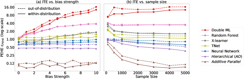
Figure 2: Results on synthetic data (5000 samples) with variable structure of the units with multiple instances of each module in each structured unit, in case of the additive parallel composition of the potential outcomes. We report $\sqrt{\epsilon_{PEHE}}$ as the strength of confounding bias increases.

5 Experiments

Modeling effects for compositional data is a novel task lacking real-world benchmark data sets. We evaluate models on synthetic data (Section 5.1) and introduce query execution and matrix operation benchmarks (Section 5.2). Data and code will be provided upon publication.

Compositional Models: We implement three compositional models based on the composition type of potential outcomes, independent or joint training of components, and access to fine-grained potential outcomes. The additive parallel (all outcomes) model is only applied to compositional data with additive parallel potential outcomes, assuming access to fine-grained potential outcomes (denoted as AO, abbreviated for all outcomes), and is implemented using a random forest and a fully connected neural network. The hierarchical (all outcomes) model’s structure is similar to the interaction graph of structured unit implemented as TreeLSTM [Tai et al., 2015], assumes separate parameters for each component, and jointly trains the models end-to-end, assuming access to fine-grained potential outcomes for individual component loss computation. The hierarchical (single outcome) model assumes access to only unit-level potential outcomes.

Baselines: We compare the performance of the compositional models with three types of baselines, selecting one or two representative estimators from each: (1) TNet, a neural network-based ITE estimator [Curth and Van der Schaar, 2021]; (2) X-learner, a meta learner that uses plug-in estimators to compute ITE, with random forest as the base model class [Künzel et al., 2019]; (3) Non-parametric Double ML [Chernozhukov et al., 2018]; and (4) Vanilla neural network and random forest-based outcome regression models. Additional details about the baselines are provided in the supplementary material.

Creation of observational data sets: All real-world data sets are experimental data collected from real-world computational systems (databases and computer programs) where we observe potential outcomes for both treatments. Observational data sets are created from experimental data of real-world computational systems by introducing confounding bias [Gentzel et al., 2021]. High-dimensional covariates are selected as biasing covariates for non-random treatment sampling. Unconfoundedness is satisfied as biasing covariates are observed. Treatment assignment dependence on biasing covariates varies between 0.1 and 0.9, creating overlap issues. Higher “bias strength" indicates higher treatment probability for certain biasing covariate values.

Table 1: Synthetic data results: We report $\sqrt{\epsilon_{PEHE}}$ across various settings: unit structure (fixed/variable), composition types (parallel/hierarchical PO), bias strength (experimental/observational), and test data distribution (WID/OOD). Difficulty in estimating ITE increases from left to right. All outcomes (AO) models assume access to fine-grained potential outcomes, and single outcomes (SO) models use only unit-level outcomes. Additive parallel models can’t estimate ITE in hierarchical PO settings. The performance advantage of compositional models becomes more evident in variable structure settings, while TNet and vanilla NN are competitive in fixed structure and parallel PO settings. Scores are normalized by average effect size, where lower is better.

Model	Fixed structure of units				Variable structure of units
	Parallel PO		Hierarchical PO		Parallel PO		Hierarchical PO
	bias=0	bias=10	bias=0	bias=10	WID	OOD	WID	OOD
Additive Parallel  (AO)	0.09	0.09	$-$	$-$	0.12	0.13	$-$	$-$
Hierarchical  (AO)	$0.37$	$0.40$	0.21	0.19	$0.44$	$0.64$	0.66	1.94
Hierarchical  (SO)	$0.90$	$1.22$	0.38	0.44	$1.12$	$1.44$	0.75	1.98
TNet  (SO)	0.16	$0.76$	$0.78$	$0.87$	$1.25$	$1.52$	$1.13$	$1.79$
X-Learner  (SO)	$0.62$	$1.97$	$0.66$	$0.75$	$1.82$	$1.81$	$1.66$	$2.24$
Double ML  (SO)	$0.73$	$9.6$	$1.94$	$3.64$	$12.88$	$16.41$	$6.64$	$3.35$
Random Forest  (SO)	$0.89$	$3.71$	$0.72$	$0.84$	$3.82$	$3.72$	$1.4$	$2.10$
Neural network  (SO)	0.27	$0.63$	$0.71$	$0.72$	$0.79$	$0.97$	$1.69$	$2.32$

5.1 Synthetic Data

We generate data sets with varying characteristics to test model performance for units with different structures and composition functions. Structured units are generated by sampling binary trees (max depth=10) with $k$=$10$ heterogeneous modules, each having $d_{j}$=$6$ features ($d$=$60$ total). The total sum of features of all components is used as a biasing covariate. Data sets vary in unit’s structure: fixed structure (each unit has exactly $k$ modules appearing once) vs. variable structure (multiple occurrences of modules per unit, variable number of distinct modules per unit). Composition types include additive parallel composition and hierarchical composition. Bias strength is varied from 0 (experimental) to 10 (observational). Results for the synthetic data experiments can be seen in Table 1 and Figure 2. Key findings include:

(1) Fixed structure vs. variable structure of units: In Table 1, we observe that the difference between the performance of the composition models (both parallel and hierarchical) and the competitive baselines (e.g., TNet, Neural Network) increases as we move from fixed structure to variable structure setting. For example, baselines TNet and Neural network are competitive to the compositional approaches in the case of fixed structure and parallel composition setting (first column in the table). This is because, in a variable structure setting, as the heterogeneity of the units increases, the fine-grained modeling of potential outcomes leads to better performance.

(2) Composition type: Encoding composition structure in model architecture improves effect estimation, especially when model architecture (parallel/hierarchical) matches the underlying composition type (parallel PO/hierarchical PO). The single-outcome hierarchical model, with only interaction structure access, is competitive with the hierarchical all-outcomes model. We observe that the error of non-compositional baselines increases as we move from parallel to hierarchical composition type (e.g., TNet’s error increases from 0.16 (column 1) to 0.78 (column 3) as we move from parallel composition to hierarchical composition, keeping everything else same (structure and bias strength).

(3) Bias strength: In Figure 2 (a) and (b), we show the performance of the models as bias strength increases, in the case of variable structure and parallel composition type. Compositional models outperform baselines (left figure) and are more sample-efficient as bias strength increases (right figure). Neural network-based models (Hierarchical, parallel, TNet, Neural Network) are less affected by increasing confounding bias than other baselines (XLearner, Random Forest, Double ML), possibly due to their ability to estimate counterfactual outcomes even with limited overlap between treatment and control populations in high-dimensional settings ($d=60$).

(4) Out-of-distribution (OOD) units: Compositional models perform better than baselines on OOD units (train: tree-depth $<$ 8, test: tree-depth $\geq$ 8), showing systematic generalization benefits in counterfactual outcome estimation.

5.2 Real-world data

Query execution in relational databases: We collect real-world query execution plans data by running 1500 SQL queries against the publicly-available Stack Overflow database under different configurations (memory size, indexing, page cost), treating configuration parameters as interventions and execution time as the potential outcome. The query plans include SQL operations like scans, joins, aggregates, and sorts as component operations. Additive parallel composition is ensured for the execution time by disabling parallelization. Results for ITE estimation for query execution data set are shown in 3 (a). Our findings include that (1) Additive parallel model estimates the effects more accurately as compared to the vanilla random forest, NN, and TNet baselines as overlap issues increase; (2) Random forest models outperform neural network-based models due to smaller sample size and execution time stochasticity. For some queries, the query execution system returns query plans with modified structures for treatment and control. In such cases, the effect is calculated assuming the corresponding structure for each treatment value. Due to this reason, we could not test baselines that do not provide counterfactual outcomes and only provide the effect estimates (e.g., X-learner, Double ML). More details about handling modified query plans are included in the supplementary material.

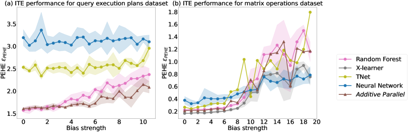
Figure 3: Results for real-world data sets: (a) Query execution data set: We observe that the parallel additive model estimates the effect more accurately as overlap issues increase. (b) Matrix operations: All baselines perform similarly for this data set.

Matrix operations data set: We generate a matrix operations data set by evaluating complex matrix expressions (units) on two different computer hardware (treatment) and store the execution time for each hardware (potential outcome). The matrix size of matrices is varied from 2 to 1000, resulting in 25000 samples. The expressions contain multiple operations, e.g., inverse, singular value decomposition, etc. We ensure that each operation is executed individually, ensuring parallel additive composition. Matrix size is used as a biasing covariate to create overlap issues. Figure 3(b) shows the results for this data set. We find that all baselines perform similarly, and compositional models show no additional benefit, potentially due to (1) the dominance of matrix multiplication operation in determining the run-time, and (2) Many operations are similar to each other, e.g., matrix multiplication, SVD, inverse, making components homogeneous and coupling their mechanisms, (3) matrix size (confounder) is affecting both unit-level and component-level outcomes, creating similar overlap issues at both levels. In contrast, synthetic and query execution data have high-dimensional covariates for unit-level outcomes, allowing better estimation with lower-dimensional component-level covariates.

6 Conclusion

The compositional approach to causal effect estimation shows promise in complex, modular systems by exploiting fine-grained information about the systems’ structure and decomposing causal queries into more fine-grained queries. The approach offers benefits such as improved sample efficiency, better overlap between treatment and control groups, enhanced out-of-distribution effect estimation, and scalable causal effect estimation for variable-size units. Future directions of this work include expanding the modular architectures to more general structured data with arbitrary graph structures and understanding the theoretical benefits of modeling complex compositions of potential outcomes.

Appendix A Broader Impacts

This paper presents work that aims to advance the field of machine learning and causal inference. There are many potential societal consequences of our work, none of which must be specifically highlighted here.

Appendix B Other examples of structured systems with compositional data

The causal questions of interest in the compositional domain are: How do the unit-level interventions impact the component-level outcomes to produce the overall unit’s outcome? Many real-world phenomena require answering such causal questions about the effect of shared interventions on different components. We provide several real-world use cases where the compositional approach can be useful to reason about the interventions’ effects and make informed, personalized decisions.

• Compiler optimization: How do different hardware architectures affect the compile time of different source codes? In this case, source code is the unit of analysis consisting of multiple program modules; hardware architecture is the unit-level intervention that can affect the compiling of different source codes differently, and compile time is the outcome of interest.

• Energy efficiency optimization: How does a state-wide mandate of shifting to more efficient electric appliances affect the monthly bill of each building in the state? Each building can be assumed to consist of various electric appliances, such that the intervention affects each kind of appliance differently, affecting the overall utility bill.

• Supply chain optimization: How is the processing time of an order affected when a supply chain company shifts to a different supplier for various parts? In this case, each order execution plan is the unit of analysis that consists of routing the information from different parties, suppliers, manufacturers, and distributors specific to each order; intervention can impact the processing time of different parties depending on the affected parts and order details.

Appendix C Composition models for individual treatment effect estimation

We first discuss the additive parallel composition model for ITE estimation using fine-grained potential-level outcomes. See Figure 1(c) for the model structure of the additive parallel compositional model.

C.1 Additive Parallel Composition Model

We first discuss the simple case of additive parallel composition to provide an intuition of model training and inference to compute ITE using fine-grained potential-level outcomes. The main idea is that the component-level models for effect estimation are instantiated specific to each unit and trained independently as we assume conditional independence among the potential outcomes given component-level features and shared treatment.

Model Training: We assume that the component models for estimating component-level potential outcomes are denoted by $\{\hat{f}_{\theta_{1}},\hat{f}_{\theta_{2}},\hat{f}_{\theta_{3}}\dots\hat{f}_{\theta_{k}}\}$, $\hat{f}_{\theta_{j}}:\mathbb{R}^{d_{j}}\times\{0,1\}\rightarrow\mathbb{R},$ each of them is parameterized by separate independent parameters $\theta_{j}$. For a given observational data set with $n$ samples, $\mathcal{D}_{F}=\{q_{i},t_{i},y_{i}\}_{i=1:N}$, we assume that we observe component-level features $\{\mathbf{x}_{ij}\}_{j=1:m_{i}}$, assigned treatment $t_{i}$ and fine-grained component-level potential outcomes $\{y_{ij}\}_{j=1:m_{i}}$ along with unit-level potential outcomes $y_{i}$. For each component model $m$, model training involves the independent learning of the parameters by minimizing the following squared loss: $\theta_{m}:=\arg\min_{\theta}\frac{1}{N_{m}}\sum_{i=1}^{N_{m}}(f_{m}(\mathbf{x}_{im},t_{i};\theta_{m})-y_{im})^{2}$. Here, $N_{m}$ denotes the total number of instances of component $m$ across all the $N$ samples. Repeated instances of the components in each unit might provide more samples to estimate the component-level potential outcomes efficiently.

Model Inference: During inference, for each unit $q_{i}=\{\mathbf{x}_{ij}\}_{j=1:m_{i}}$, depending on the presence of the number and kind of each component $\{1,2,\dots m_{i}\}$ in $G_{i}$, component index $l$ of distinct component corresponding to each component instance $j$ is obtained. Then, both the potential outcomes are computed $\hat{y}_{ij}(1)=\hat{f}_{\theta_{l}}(\mathbf{x}_{ij},1)$, $\hat{y}_{ij}(0)=\hat{f}_{\theta_{l}}(\mathbf{x}_{ij},0)$. Assuming additive composition, $\hat{y}_{i}(1),\hat{y}_{i}(0)=\sum_{j}^{m_{i}}\hat{f}_{\theta_{l}}(\mathbf{x}_{ij},1),\sum_{j}^{m_{i}}\hat{f}_{\theta_{l}}(\mathbf{x}_{ij},0)$. ITE estimate for each unit $i$ by additive parallel composition model is given by $\hat{\tau}(q_{i})=\hat{y}_{i}(1)-\hat{y}_{i}(0)$. The additive parallel composition model explicitly encodes the conditional independence of the distribution of component-level potential outcomes given its causes (component-level features and treatments). This is similar to assuming the causal Markov assumption in the graphical models [Pearl, 2009], and independent training of the parameters of component models is inspired by the independence of mechanisms among underlying components’ assumption [Peters et al., 2017]. Generally, the aggregation function can be non-additive and a complex non-linear function of the potential outcomes. Assuming that the aggregation function is the same across all data instances and parameterized by ${\phi}$, the function’s parameters can be learned from the training data by minimizing the following objective: $\phi:=\arg\min_{\phi}\frac{1}{N}\sum_{i=1}^{N}(g(y_{i1}(t),y_{i2}(t),\dots{y_{i{m_{i}}}(t)});\phi_{j})-y_{i}(t))^{2}$. ( Algorithms 1, 2) provide more details.

C.2 Hierarchical Composition Model

In hierarchical composition, we assume the same information about the components is available in parallel composition. The main difference is that we assume that the potential outcomes of components can directly affect each other, and tree-like interaction structure $G_{i}$ denotes the composition structure of the potential outcomes. More specifically, the potential outcome of each component is computed using input features of that component, shared unit-level treatment, and potential outcomes of the children’s components. Potential outcomes of the children’s components are passed as input to the components in a hierarchical fashion, and the potential outcome of the root node is treated as the unit-level outcome. In the hierarchical composition model, component models are trained jointly end-to-end to estimate the unit-level potential outcomes. Compared to the parallel composition, the hierarchical composition doesn’t make any explicit assumption about the independence among the potential outcomes and captures the complex interactions among them. These modular and recursive architectures are commonly used in associational machine learning to model the natural language parse trees and structured images for structured prediction tasks [Socher et al., 2011, Andreas et al., 2016].

Model Training: For a unit $i$, a modular architecture consisting of $m_{i}$ component models is instantiated with the same input and output structure as $G_{i}$. The potential outcomes are computed using the post-order traversal of the tree $G_{i}$. The potential outcome for a model $m$ is computed as $\hat{y}_{ij}=\hat{f}_{\theta_{m}}(\mathbf{x}_{ij},t_{i},\hat{y}_{i{j-1}},\hat{y}_{i{j-2}};\theta_{m})$, where $\hat{y}_{i{j-1}}$ and $\hat{y}_{i{j-2}}$ are the outcomes of the children nodes of each component (assuming binary tree). If a component is the leaf node, then the potential outcome is computed just as a function of the input features and the intervention, i.e., $\hat{y}_{ij}=\hat{f}_{\theta_{m}}(\mathbf{x}_{ij},t_{i},\theta_{m})$. The total loss for each unit $i$ is computed as the sum of the loss of each component $\sum_{j}^{m_{i}}(\hat{y}_{ij}-y_{ij})^{2}$ and gradients are updated for the parameters of each component.

Model Inference: To compute ITE for a unit $i$, a modular architecture consisting of $m_{i}$ component models is instantiated with the same input and output structure as $G_{i}$, and the potential outcome of the root module is taken as the unit level component, i.e., $\hat{y}_{i}(t)=\hat{y}_{im_{i}}(t)$. ITE estimate for each unit $i$ by hierarchcial composition model is given by $\hat{\tau}(q_{i})=\hat{y}_{i}(1)-\hat{y}_{i}(0)$.

Algorithm 3, (4) provide more details about hierarchical composition model training and inference.

Unobserved component-level potential outcomes: There might be cases when we only observe the unit-level outcome. In that case, it is possible to have another version of the hierarchical composition model when we don’t have access to the fine-grained potential outcome and only have information about the component-level features and the interaction graph representing the computation structure of the unit. In that case, we can jointly train all the components, and gradients can mainly be computed based on unit-level outcome prediction loss. We demonstrate the performance of both versions of hierarchical composition models in our experiments.

C.3 Algorithms to estimate individual treatment effects

C.3.1 Parallel Composition Model:

Algorithm 1 Parallel Composition: Training

1:  Input: Factual data set: $\mathcal{D}_{F}=\{q_{i}:\{\mathbf{x}_{ij}\}_{j=1:m_{i}},t_{i},y_{i},\{y_{ij}\}_{j=1:m_{i}}\}_{i=1:n}$, number of distinct components $k$.

2:  Result: Learned aggregation function $\hat{g}_{\phi}$ and potential outcome models for each component: $\{\hat{f}_{\theta_{1}},\hat{f}_{\theta_{2}},\hat{f}_{\theta_{3}}\dots\hat{f}_{\theta_{k}}\}$

3:  Procedure:

4:  $\mathcal{D}_{1}\leftarrow\{\},\mathcal{D}_{2}\leftarrow\{\},\mathcal{D}_{3}\leftarrow\{\}\dots\mathcal{D}_{k}\leftarrow\{\}$

5:  for $i=1$ to ${n}$ do

6:     for $j=1$ to ${m_{i}}$ do

7:        $l\leftarrow component\_index(j)$   index of distinct component for $j^{th}$ component instance.

8:        $\mathcal{D}_{l}\leftarrow\mathcal{D}_{l}\cup\{\mathbf{x}_{ij},t_{i},y_{i}\}$

9:     end for

10:  end for

11:  for $l=1$ to ${k}$ do

12:     $N_{l}\leftarrow len(\mathcal{D}_{l})$ 

13:     $\theta_{l}:=\arg\min_{\theta}\frac{1}{N_{l}}\sum_{i=1}^{N_{l}}(f_{l}(\mathbf{x_{i}},t_{i};\theta_{l})-y_{i})^{2}$   independent training of all the component models.

14:  end for

15:  $\phi:=\arg\min_{\phi}\frac{1}{N}\sum_{i=1}^{N}(g(y_{i1},y_{i2},\dots{y_{i{m_{i}}}});\phi_{j})-y_{i})^{2}$

Algorithm 2 Parallel Composition: Inference

1:  Input: Test data set: $\mathcal{D_{T}}=\{q_{i}:\{\mathbf{x}_{ij}\}_{j=1:m_{i}}\}_{i=1:n}$, learned aggregation function model $\hat{g}_{\phi}$ and potential outcome models for each component: $\{\hat{f}_{\theta_{1}},\hat{f}_{\theta_{2}},\hat{f}_{\theta_{3}}\dots\hat{f}_{\theta_{k}}\}$,

2:  Result: ITESamples

3:  Procedure:

4:  $ITESamples\leftarrow\{\}$

5:  for $i=1$ to ${n}$ do

6:     for $j=1$ to ${m_{i}}$ do

7:        $l\leftarrow component\_index(j)$

8:        $\hat{y}_{ij}(1)=\hat{f}_{\theta_{l}}(\mathbf{x}_{ij},1)$

9:        $\hat{y}_{ij}(0)=\hat{f}_{\theta_{l}}(\mathbf{x}_{ij},0)$

10:     end for

11:     $\hat{y}_{i}(1)=\hat{g}_{\phi}(\hat{y}_{ij}(1),\hat{y}_{ij}(1)\dots\hat{y}_{im_{i}}(1))$ 

12:     $\hat{y}_{i}(0)=\hat{g}_{\phi}(\hat{y}_{ij}(0),\hat{y}_{ij}(0)\dots\hat{y}_{im_{i}}(0)$) 

13:     $\hat{\tau}(q_{i})=\hat{y}_{ij}(1)-\hat{y}_{i}(0)$

14:     $ITESamples\leftarrow ITESamples\cup\{(q_{i},\hat{\tau}(q_{i}))\}$

15:  end for

C.3.2 Hierarchical Composition Model

Algorithm 3 Hierarchical Composition: Training

1:  Input: Factual data set: $\mathcal{D}_{F}=\{q_{i}:\{\mathbf{x}_{ij}\}_{j=1:m_{i}},t_{i},y_{i},\{y_{ij}\}_{j=1:m_{i}}\}_{i=1:n}$, number of distinct components $k$.

2:  Result: Learned potential outcome models for each component: $\{\hat{f}_{\theta_{1}},\hat{f}_{\theta_{2}},\hat{f}_{\theta_{3}}\dots\hat{f}_{\theta_{k}}\}$

3:  while not converged do

4:     $loss\_1,loss\_2,loss\_3,loss\_k=0$

5:     for $i=1$ to ${n}$ do

6:        Get the order of the components in which input is processed by using post-order traversal of the tree $G_{i}$.

7:        $orderedList\leftarrow post\_order\_traversal(G_{i})$

8:        for component $j$ in $orderedList$ do

9:           $l\leftarrow component\_index(j)$

10:           // Potential outcome of a component depends on the potential outcome of the children components according to graph $G_{i}$ (assuming binary tree)

11:           if component $m$ has children in $G_{i}$ then

12:              $\hat{y}_{ij}=\hat{f}_{\theta_{l}}(\mathbf{x}_{ij},t_{i},\hat{y}_{i{j-1}},\hat{y}_{i{j-2}};\theta_{l})$

13:           else if component $l$ is a leaf operation then

14:              $\hat{y}_{ij}=\hat{f}_{\theta_{l}}(\mathbf{x}_{ij},t_{i},\theta_{l})$

15:           end if

16:           $loss\_l=loss\_l+(\hat{y}_{ij}-y_{ij})^{2}$

17:        end for

18:     end for

19:     Calculate gradients for the parameters for each module

20:     for $l=1$ to ${k}$ do

21:        $\delta_{l}\leftarrow\triangle_{\theta_{l}}\frac{1}{N_{l}}loss\_l$ 

22:        $\theta_{l}\leftarrow\theta_{l}-\alpha\delta_{l}$ joint training of all the component models.

23:     end for

24:     Check convergence criterion

25:  end while

Algorithm 4 Hierarchical Composition: Inference

1:  Input: Test data set: $\mathcal{D_{T}}=\{q_{i}:\{\mathbf{x}_{ij}\}_{j=1:m_{i}}\}_{i=1:n}$, learned potential outcome models for each component: $\{\hat{f}_{\theta_{1}},\hat{f}_{\theta_{2}},\hat{f}_{\theta_{3}}\dots\hat{f}_{\theta_{k}}\}$,

2:  Result: ITESamples

3:  Procedure:

4:  $ITESamples\leftarrow\{\}$

5:  for $i=1$ to ${n}$ do

6:     Get the order of the operation in which input is processed by post-order traversal of the tree

7:     $orderedList\leftarrow post\_order\_traversal(G_{i})$

8:     for component $j$ in $orderedList$ do

9:        $l\leftarrow component\_index(j)$

10:        $\hat{y}_{ij}=\hat{f}_{\theta_{l}}(\mathbf{x}_{ij},t_{i},\hat{y}_{i{j-1}},\hat{y}_{i{j-2}};\theta_{l}),$

11:     end for

12:     $\hat{y}_{i}(1)=\hat{y}_{im_{i}}$, get the potential outcome of the root component in $G_{i}$

13:     $\hat{y}_{i}(0)=\hat{y}_{im_{i}}$, get the potential outcome of the root component in $G_{i}$

14:     $\hat{\tau}(q_{i})=\hat{y}_{i}(1)-\hat{y}_{i}(0)$

15:     $ITESamples\leftarrow ITESamples\cup\{(q_{i},\hat{\tau}(q_{i}))\}$

16:  end for

Appendix D Theoretical Proofs

D.1 Identifiability of individual treatment effects in case of additive parallel composition

Theorem D.1.

The CATE estimand for the structured units in case of additive parallel composition is equal to the additive composition of the component-level CATE estimands and is identified by the following estimand.

$$\tau(q)=\sum_{j=1}^{m_{i}}\mathbb{E}[y_{j}|\mathbf{x_{j}},t=1]-\mathbb{E}[y_{j}|\mathbf{x_{j}},t=0]$$ (3)

If we make the following assumptions:

Assumption E.

Parallel composition assumes that the ground-truth component-level potential outcomes are conditionally independent of potential outcomes of other components given component-level covariates and treatment: $P(Y_{a}(t)|X_{a},T)\perp P(Y_{b}(t)|X_{b},T)\ \forall a,b\in\{1,2,\dots k\},a\neq b$.

Assumption F.

Additivity assumes that ground-truth component-level potential outcomes add to generate the ground-truth unit-level potential outcome, i.e., $Y_{i}(1)=\sum_{j}^{m_{i}}Y_{ij}(1)$, $Y_{i}(0)=\sum_{j}^{m_{i}}Y_{ij}(0)$.

Assumption G.

Component-level unconfoundedness assumes that unconfoundedness holds for the component level potential outcomes, i.e., $Y_{ij}(1),Y_{ij}(0)\perp T_{i}|\mathbf{X}_{ij}$.

Assumption H.

Component-level overlap assumes that overlap holds for the component level covariates, i.e., $0<p(t=1|\mathbf{x}_{j})<1$.

Assumption I.

Component-level consistency assumes that consistency holds for the component level covariates, i.e., $y_{ij}=Y_{ij}(0)|t=0$ and $y_{ij}=Y_{ij}(1)|t=1$.

Proof.

The individual-level treatment effect (ITE) estimand for structured units is defined as

$$\tau(q)=\mathbb{E}[Y_{i}(1)-Y_{i}(0)|Q_{i}=q]=\mathbb{E}[Y_{i}(1)-Y_{i}(0)|Q_{i}=(G_{i},\{\mathbf{x}_{ij})\}_{j=1:m_{i}}]$$

Assuming additivity F, we get

$$\tau(q)=\mathbb{E}[\sum_{j}^{m_{i}}Y_{ij}(1)-\sum_{j}^{m_{i}}Y_{ij}(0)|Q_{i}=(G_{i},\{\mathbf{x}_{ij})\}_{j=1:m_{i}}]$$

Due to the linearity of the expectation, we get the following:

$$\tau(q)=\mathbb{E}[\sum_{j}^{m_{i}}Y_{ij}(1)|Q_{i}=\{\mathbf{x}_{ij}\}_{j=1:m_{i}}]-\mathbb{E}[\sum_{j}^{m_{i}}Y_{ij}(0)|Q_{i}=\{\mathbf{x}_{ij}\}_{j=1:m_{i}}]$$

$$\tau(q)=\sum_{j}^{m_{i}}\mathbb{E}[Y_{ij}(1)|Q_{i}=\{\mathbf{x}_{ij}\}_{j=1:m_{i}}]-\sum_{j}^{m_{i}}\mathbb{E}[Y_{ij}(0)|Q_{i}=\{\mathbf{x}_{ij}\}_{j=1:m_{i}}]$$

Assuming parallel composition E, we get that the computation of potential outcomes does not depend on the interaction graph $G_{i}$ and only depends on the component-level features.

$$\tau(q)=\sum_{j}^{m_{i}}\mathbb{E}[Y_{ij}(1)|\mathbf{x}_{ij}]-\mathbb{E}[Y_{ij}(0)|\mathbf{x}_{ij}]$$

Assuming component-level unconfoundedness G

$$\tau(q)=\sum_{j}^{m_{i}}\mathbb{E}[Y_{ij}(1)|\mathbf{x}_{ij},t=1]-\mathbb{E}[Y_{ij}(0)|\mathbf{x}_{ij},t=0]$$

Assuming component-level consistency I

$$\tau(q)=\sum_{j}^{m_{i}}\mathbb{E}[Y_{ij}|\mathbf{x}_{ij},t=1]-\mathbb{E}[Y_{ij}|\mathbf{x}_{ij},t=0]$$

Component-level overlap H ensures that the estimate is identified using observational data. ∎

I.1 Decomposition of the generalization error of the additive parallel compositional model

The treatment effect estimate of a model $\hat{f}$ for unit $q$ is $\hat{\tau}_{\hat{f}}(q)=\hat{f}(q,1)-\hat{f}(q,0)$. We measure the performance using precision in the estimation of heterogeneous effect (PEHE) loss [Hill, 2011], which is defined by the mean squared error difference in the estimated effect and the ground truth effect for a population of units sampled from density $\epsilon_{PEHE}(\hat{f})=\mathbb{E}[(\hat{\tau}_{\hat{f}}(q)-\tau(q))^{2}]$. Using the result of the Theorem 4.1, it can be easily shown that the error of the additive parallel compositional model can be decomposed into the sum of the errors of individual component models ($\hat{f}_{\theta_{j}}$) and pair-wise covariance between the errors of the component models, similar to the generalization error analysis of the ensemble models [Ueda and Nakano, 1996]. We provide the derivation in the supplementary material. Intuitively, if all the component potential functions are the same, then the errors of the component models would be highly correlated, and errors would aggregate. The more heterogeneous the components are, the more benefits there are from the compositional approach.

$$\epsilon_{PEHE}(f_{add})=\sum_{j=1}^{m_{i}}{\epsilon_{PEHE}(\hat{f}_{\theta_{j}})}+\sum_{j}\sum_{k,k\neq j}\sqrt{{\epsilon_{PEHE}(\hat{f}_{\theta_{j}})}}\sqrt{{\epsilon_{PEHE}(\hat{f}_{\theta_{k}})}}$$ (4)

Derivation:

$$\hat{\tau}_{\hat{f}}(q)=\hat{f}(q,1)-\hat{f}(q,0)$$

For parallel, additive model, using Theorem D.1, we get:

$$\hat{\tau}_{\hat{f}}(q)=\sum_{j=1}^{m_{i}}\hat{\tau}_{\hat{f}}(\mathbf{x_{j}})=\sum_{j=1}^{m_{i}}\mathbb{E}[y_{j}|\mathbf{x_{j}},t=1]-\mathbb{E}[y_{j}|\mathbf{x_{j}},t=0]$$

$$=\sum_{j=1}^{m_{i}}\hat{f}(\mathbf{x}_{j},1)-\hat{f}(\mathbf{x}_{j},0)$$

PEHE for the additive model for distribution of units $p(q)$ By expanding the square of the terms, we get.

$$\epsilon_{PEHE,p}(f_{add})=\mathbb{E}_{p(q)}[\big{[}\sum_{j}^{m_{i}}\hat{\tau}(x_{j})-\tau(x_{j})\big{]}^{2}]$$

$$=\mathbb{E}_{p(q)}[\sum_{j=1}^{m}\big{[}\hat{\tau}(x_{j})-\tau(x_{j})\big{]}^{2}]+\mathbb{E}_{p(q)}[\sum_{j}\sum_{k,k\neq j}(\hat{\tau}_{j}-\tau_{j})(\hat{\tau}_{k}-\tau_{k})]$$

$$=\sum_{j=1}^{m_{i}}{\epsilon_{PEHE}(\hat{f}_{\theta_{j}})}+\sum_{j}\sum_{k,k\neq j}\sqrt{{\epsilon_{PEHE}(\hat{f}_{\theta_{j}})}}\sqrt{{\epsilon_{PEHE}(\hat{f}_{\theta_{k}})}}$$

I.1.1 Decomposition of PEHE error into factual and counterfactual errors:

For a unit $q$, with observed treatment $t$, observed potential outcome $y$ and unobserved counterfactual outcome $y_{CF}$, the factual $(\epsilon_{F})$ and counterfactual errors $(\epsilon_{CF})$ are defined as [Shalit et al., 2017]:

$$\epsilon_{F,p}(\hat{f})=\mathbb{E}_{p(q,t)}[(\hat{f}(q)-y)^{2}]$$

$$\epsilon_{CF,p}(\hat{f})=\mathbb{E}_{p(q,1-t)}(\hat{f}(q,1-t)-y_{CF})^{2}$$

The existing generalization error upper bound for $\epsilon_{PEHE}$ is given by [Shalit et al., 2017]:

$$\epsilon_{PEHE}\leq 2(\epsilon_{F}+\epsilon_{CF})$$ (5)

It was further shown by [Shalit et al., 2017] that the counterfactual error can be upper bounded by the sum of factual error and distribution mismatch term between treatment $P(X=x|T=0)$ and control populations $P(X=x|T=1)$. Note that the distribution mismatch was defined in Shalit et al. [2017] concerning the well-defined representation functions for the covariates. For simplicity, we define it by considering the original density of the covariates. Suppose $u$ is the probability of treatment $p(t=1)$ in the observational data. In that case, $D$ denotes the metric to measure the distribution mismatch between the control and treatment populations, e.g., the integral probability metric distance, and $\alpha$ is a normalization constant for a metric to be well-defined.

$$\epsilon_{CF}\leq u\epsilon^{t=0}_{F}+(1-u)\epsilon_{F}^{t=1}+\alpha D(p^{t=1}_{x},p^{t=0}_{x})$$ (6)

Similarly, we can decompose the factual errors in terms of factual errors of the component models.

$$\epsilon_{F}(f_{add})=\sum_{j=1}^{m_{i}}{\epsilon_{j}}_{F}+\sum_{j}\sum_{k,k\neq j}\sqrt{{\epsilon_{j}}_{F}}\sqrt{{\epsilon_{k}}_{F}}$$

$$\epsilon_{CF}(f_{add})=\sum_{j=1}^{m_{i}}{\epsilon_{j}}_{CF}+\sum_{j}\sum_{k,k\neq j}\sqrt{{\epsilon_{j}}_{CF}}\sqrt{{\epsilon_{k}}_{CF}}$$

Suppose we assume that the ground-truth potential outcome functions for the components are independent of each other, independence of mechanisms of components, i.e., components are heterogeneous. In that case, the PEHE error of the additive model reduces to the sum of the PEHE errors of individual components in equation 4. If we apply the error bounds for PEHE 5 and error bounds for counterfactual errors 6 on the error of the component models, we get the below upper bound for the error of the additive parallel model with independent component potential functions.

$$\epsilon_{PEHE,p}(f_{add})\leq\sum_{j}^{m_{i}}\underbrace{{\epsilon_{j}}_{F}^{t=1}+{\epsilon_{j}}_{F}^{t=0}}_{factual\_error\_j}+\underbrace{\alpha D(p^{t=1}_{\mathbf{x_{j}}},p^{t=0}_{\mathbf{x_{j}}})}_{distribution\_mismatch\_j}$$ (7)

I.2 Generalization error of additive parallel compositional model for prediction task

The generalization error of the estimator for each component $f_{C_{j}}$ on the test set $X_{0j}$ can be written as below. Let’s assume that $D_{j}^{N}=\{X_{j}^{1:N},Y_{j}^{1:N}\}$ denotes the training set for the component $C_{j}$ of size $N$. We assume that each component has irreducible additive noise with standard deviation $\sigma_{j}$.For simplicity, we assume that each component is trained on same data size $N$.

We assume that the overall estimate of the modular model is the additive composition of the estimates from individual estimators.

$$f^{k}_{M}(X_{1},X_{2},\dots X_{k})=\sum_{j=1}^{k}f_{j}(X_{j};D^{N}_{j})$$ (8)

Let’s assume that the output of each component model is generated using the following equation

$$Y_{j}=g_{j}(X_{j})+\sigma_{g}$$

Using bias-variance decomposition of the generalization error, we get:

$$R_{f_{j}}=\mathbb{E}_{X_{0j}}\bigl{\{}Var(f_{j}|X_{0j})+Bias(f_{j}|X_{j})^{2}\bigl{\}}+\sigma_{j}^{2}$$ (9)

Similar to the analysis of the ensemble models, the generalization error of the component level model on the test set $X_{0}=\{X_{01},X_{02}\dots X_{0k}\}$ can be decomposed into the bias, variance, and covariance of the individual component estimators Ueda and Nakano [1996]. The difference between the ensemble models and the additive parallel compositional model is that in ensemble models, each estimator is trained on the same training data. The estimate is the weighted average of individual estimates. In contrast, in the compositional model, each estimator is trained on data from different components, and the overall estimate is additive rather than the average of the individual estimates. This leads to the variance addition from difference component models rather than the variance reduction as seen in ensemble models.

Theorem I.1.

The generalization error $(R_{f^{k}_{M}})$ of the additive parallel model $f^{k}_{M}$ consisting of k components on the test set $X_{0}=\{X_{01},X_{02}\dots X_{0k}\}$ can be decomposed into the sum of variances ($\overline{Var}(X_{0})$), sum of biases ($\overline{Bias}(X_{0}))$, and sum of pairwise covariance ($\overline{Cov}(X_{0})$) of the individual component estimators $f_{j}$. $\sigma_{j}$ denotes the standard deviation of irreducible additive noise for the outcome of each component.

$$R_{f^{k}_{M}}=\mathbb{E}_{X_{0}}[\overline{Var}(X_{0})+\overline{Cov}(X_{0})+\overline{Bias}(X_{0})^{2}]+\sum_{j}\sigma_{j}^{2}$$

, where

$$\overline{Var}(X_{0})=\sum_{j=1}^{k}Var(f_{j}|X_{0j})$$

$$\overline{Bias}(X_{0})=\sum_{j=1}^{k}Bias(f_{j}|X_{0j})$$

$$\overline{Cov}(X_{0})=\sum_{j}\sum_{j\textquoteright\neq j}Cov(f_{j},f_{j}\textquoteright|X_{0j},X_{0j^{\prime}})$$

Proof.

Let $R_{f^{k}_{M}}$ denote the generalization error of the additive modular model whose estimate is given by 8. Using bias/variance decomposition Geman et al. [1992] of the modular model’s estimator, we have.

$$R_{f^{k}_{M}}=\mathbb{E}_{X_{0}}\bigl{\{}Var(f^{k}_{M}|X_{0})+Bias(f^{k}_{M}|X_{0})^{2}\bigl{\}}+\sigma^{2}$$

$$Var(f^{k}_{M}|X_{0})=\mathbb{E}_{D_{1}^{N},\dots D_{k}^{N}}\big{[}\sum_{j=1}^{k}f_{j}(X_{0j};D^{N}_{j})-\mathbb{E}_{D_{1}^{N},\dots D_{k}^{N}}[\sum_{j=1}^{k}f_{j}(X_{0j};D^{N}_{j})]\big{]}^{2}$$

$$=\sum_{j=1}^{k}\mathbb{E}_{D_{j}^{N}}[f_{j}-\mathbb{E}_{D_{j}^{N}}[f_{j}]]^{2}+\sum_{j}\sum_{j\textquoteright\neq j}\mathbb{E}_{D_{j}^{N},D_{j^{\prime}}^{N}}[f_{j}-\mathbb{E}_{D_{j}^{N}}[f_{j}]][f_{j^{\prime}}-\mathbb{E}_{D_{j^{\prime}}^{N}}[f_{j^{\prime}}]]$$

$$=\overline{Var}(X_{0})+\overline{Cov}(X_{0})$$

$$Bias(f^{k}_{M}|X_{0})=\mathbb{E}_{D_{1}^{N},\dots D_{k}^{N}}[\sum_{j=1}^{k}f_{j}(X_{0j};D^{N}_{j})-g_{j}(X_{0j}]$$

$$=\sum_{j=1}^{k}\mathbb{E}_{D_{j}^{N}}[f_{j}-g_{j}]=\sum_{j=1}^{k}Bias(f_{j}|X_{0j})=\overline{Bias}(X_{0})$$

Therefore,

$$R_{f^{k}_{M}}=\mathbb{E}_{X_{0}}[\overline{Var}(X_{0})+\overline{Cov}(X_{0})+\overline{Bias}(X_{0})^{2}]+\sum_{j}\sigma_{j}^{2}$$

∎

Appendix J Experiments

Implementation of the Compositional Models

1. Additive Parallel Models: We implement an additive parallel model using two model classes: random_forest and neural_network. A three-layer, fully connected MLP architecture was used for neural network models with hidden layer dimension = 64 and ReLU activations. Models were trained using Adam Optimizer with a learning rate of $0.01$.

2. Hierarchical Composition Models: TreeLSTM architecture was used with a hidden dimension size = 64 and batch size = 32 for each component. Models were trained using Adam optimizer with a learning rate of $0.01$. For all outcomes of the hierarchical model, total loss for all the components was optimized, while for the single-outcome model, loss for only unit-level potential outcome was optimized.

Baselines: X-learner and non-parametric double machine learning implementation is from Econml library and random forests were used as the base models. TNet [Curth and Van der Schaar, 2021] implementation is taken from the Github repository catenets.

J.1 Synthetic Data Generation:

We generate data sets with varying characteristics to test model performance for units with different structures and composition functions. Structured units are generated by sampling binary trees (max depth=10) with $k$=$10$ heterogeneous modules, each having $d_{j}$=$6$ features ($d$=$60$ total). The total sum of features of all components is used as a biasing covariate to create overlap issues. The covariate distribution for each component is sampled from a multivariate Gaussian distribution with a mean ranging between 0 and 3 and covariance ranging between 0 and 3. The potential outcomes for each treatment is a quadratic function with different parameters for each treatment to generate heterogeneous treatment effects. For fixed structure data generation, the depth of the tree is fixed to $10$ so that every unit has exactly the same number and kind of components. For the variable structure setting, the depth of the tree randomly varies between $4$ and $10$, and components are sampled with replacement. Every non-leaf node has another component, such as children, and component-specific features, such as children. Potential Outcome is simulated for each component for each treatment as a function of input features and treatment for parallel composition and as a function of input features, treatment, and potential outcome of the children components.

J.2 Real-world data

We first collect 10000 most popular user-defined Math Stack Overflow queries. We install a PostgreSQL 14 database server and load a 50 GB version of the publicly available Stack Overflow Database. We then run these queries with different combinations of the configuration parameters listed in Table 2. In all our experiments, our queries were executed with PostgreSQL 14 database on a single node with an Intel 2.3 GHz 8-Core Intel Core i9 processor, 32GB of RAM, and a solid-state drive. PostgreSQL was configured to use a maximum of 0 parallel workers to ensure non-parallelized executions so that additive assumption about operations is satisfied (max_parallel_workers_per_gather = 0). Before each run of the query, we begin from the cold cache by restarting the server to reduce caching effects among queries. Many database management systems provide information about the query plans as well as actual execution information through convenient APIs, such as EXPLAIN ANALYZE queries. Usually, the total run-time of each operation, along with children’s operations, is reported by Postgres. To model the behavior of each component operation, we require the individual run-time of each component operation. This is calculated using publicly available query plan explainer websites such as this. We mainly model the query plans with the following operations — Sequential Scan, Index Scan, Sort, Aggregate, Hash, Hash Join as the occurrence of these operations in collected query plans was good, providing a large number of samples to learn the models from data. For ITE estimation experiments, we select $1500$ query plans in which effect sizes were significant and were actually a result of the intervention rather than random variation in the run-time due to the stochastic nature of the database execution system. Each SQL query is run 5 times, and the median execution time is taken as the outcome. We use data for memory size increase intervention.

J.3 Matrix Operation data generation

We generate a matrix operations data set by evaluating complex matrix expressions (units) on two different computer hardware (treatment) and store the execution time for each hardware (potential outcome). The matrix size of matrices is varied from 2 to 1000, resulting in 25000 samples. The expressions contain multiple operations, e.g., inverse, singular value decomposition, etc. We ensure that each operation is executed individually, ensuring parallel additive composition. Matrix size is used as a biasing covariate to create overlap issues.

Working Memory	Temp Buffers	Indices	Page Cost
64 KB	800 KB	No indexing	High random page cost
2 MB	8 MB	Primary key indexing	Equal random and sequential page cost
50 MB	100 MB	Secondary key indexing	High sequential page cost

Table 2: Realistic interventions for causal effect estimation

J.4 Covariates used for query execution data for model training

See 3 for the information about the high-dimensional features and component-specific features used for training query execution plans

Model	Component	Training features	Outcome
Random Forest, Neural Network, TNet		num_Sort, num_Hash_Join, num_Seq_Scan, num_Hash, num_Index_Scan, num_Aggregate, num_complex_ops, Sort_input_rows, Hash Join_input_rows, Hash Join_left_plan_rows, Hash Join_right_plan_rows, Seq Scan_input_rows, Hash_input_rows, Index Scan_input_rows, Aggregate_input_rows	total_execution_time
Compositional	Sequential Scan	Seq_Scan_input_rows, Seq_Scan_plan_rows	seq_scan_execution_time
Compositional	Index Scan	Index_Scan_input_rows, Index_Scan_plan_rows	index_scan_execution_time
Compositional	Hash	Hash_input_rows, Hash_plan_rows	hash_execution_time
Compositional	Hash Join	Hash_Join_left_input_rows, Hash_Join_right_input_rows, Hash_Join_plan_rows	hash_join_execution_time
Compositional	Sort	Sort_input_rows, Sort_plan_rows	sort_execution_time
Compositional	Aggregate	Aggregate_input_rows, Aggregate_plan_rows	aggregate_execution_time

Table 3: Training input and output features used by associational, SCM, and modular models for both simulated and real-world query plans

J.5 Experiment 5: Causal effect estimation of realistic interventions on observational dataset:

We apply following kind of interventions to the query plans — (1) Increasing memory: In this, we increase the size of working memory from 64 KB to 50 MB before running the query. Based on the prior knowledge, this can cause query plans to use more efficient sorting methods, such as quick sort, as compared to external sort (on disk), which can cause the hash operation to use bigger hash tables; 2) Adding indices: In this intervention, we add indexing data structures on foreign keys of the database tables, encouraging query planners to propose more plans with index scans as compared to sequential scans; (3) Adding indices and increasing memory: In this, we apply both interventions together, allowing for complex interactions due to multiple treatments. Ground truth causal effects and effects after introducing observational bias for all the interventions are shown in Figure 4 below. We use sort output rows to bias the treatment in case of increasing memory intervention. For indices, we use scan rows as a biasing covariate, and for both indices and memory intervention, we use total output rows as a biasing covariate.

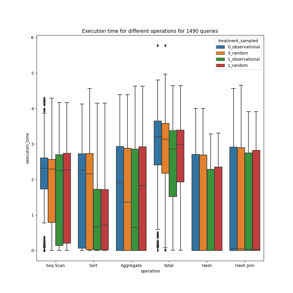
Figure 4: Ground-truth causal effect estimate of increasing memory for experimental data (random) and observational data created with bias strength 1. 0: low memory, 1: high memory. We can see that increasing memory has the most effect on Sort and aggregate operation and the least effect on the sequential scan.

J.5.1 Change in query plan as a result of interventions on configuration parameters:

For some interventions on the configuration parameters and for some queries, the query planner doesn’t return the same query plan. It returns the query plan with a changed structure as well as modified features of the components. This makes sense as that is the goal of query optimizers to compare different plans as resources change and find the most efficient plan. For example, increasing the working memory often causes query planners to change the ordering of Sort and aggregate operations, changing the structure as well as inputs to each component. These interventions are different from standard interventions in causal inference in which we assume that the covariates of the unit remain the same (as they are assumed to be pre-treatment) and treatment only modifies the outcome. In this case, a few features of the query plan are modified as a result of the intervention (and thus are post-treatment), while other features remain the same. Prediction of which features would change is part of learning the behavior of the query planner under interventions. In this work, we have mostly focused on learning the behavior of the query execution engine and assumed that the query planner is accessible to us. For simplicity, we assume that we know of the change in structure as a result of the intervention for both models. We leave the learning of the behavior of query optimizers under interventions for future work. This case provides another challenge for the task of causal effect estimation, even in the case of randomized treatments (bias strength = 0); due to the modified features of the query plans, the distribution of features in control and treatment populations might differ, providing an inherent observational bias in the dataset coming from the query optimizer. As long as we provide the information about modified query plans for both models, we believe that our comparisons are fair. For changed query structure, CATE estimand can be thought of as conditional on the same query but two different query plans.

$$\tau(Q_{i})=\mathbb{E}[Y_{i}(1)-Y_{i}(0)|Q_{i}]$$

$$\tau(Q_{i})=\mathbb{E}[\mathbb{E}[Y_{i}(1)|Q_{p_{i}}(1)]-\mathbb{E}[Y_{i}(0)|Q_{p_{i}}(0)]]$$

References

- Andreas et al. [2016] J. Andreas, M. Rohrbach, T. Darrell, and D. Klein. Neural module networks. In Proceedings of the IEEE conference on computer vision and pattern recognition, pages 39–48, 2016.
- Athey and Imbens [2016] S. Athey and G. Imbens. Recursive partitioning for heterogeneous causal effects. Proceedings of the National Academy of Sciences, 113(27):7353–7360, 2016.
- Boopathy et al. [2024] A. Boopathy, S. Jiang, W. Yue, J. Hwang, A. Iyer, and I. R. Fiete. Breaking neural network scaling laws with modularity, 2024. URL https://openreview.net/forum?id=unE3TZSAVZ.
- Bottou et al. [2013] L. Bottou, J. Peters, J. Quiñonero-Candela, D. X. Charles, D. M. Chickering, E. Portugaly, D. Ray, P. Simard, and E. Snelson. Counterfactual reasoning and learning systems: The example of computational advertising. Journal of Machine Learning Research, 14(11), 2013.
- Callebaut and Rasskin-Gutman [2005] W. Callebaut and D. Rasskin-Gutman. Modularity: Understanding the Development and Evolution of Natural Complex Systems. MIT press, 2005.
- Chernozhukov et al. [2018] V. Chernozhukov, D. Chetverikov, M. Demirer, E. Duflo, C. Hansen, W. Newey, and J. Robins. Double/debiased machine learning for treatment and structural parameters, 2018.
- Curth and Van der Schaar [2021] A. Curth and M. Van der Schaar. Nonparametric estimation of heterogeneous treatment effects: From theory to learning algorithms. In International Conference on Artificial Intelligence and Statistics, pages 1810–1818. PMLR, 2021.
- Curth et al. [2024] A. Curth, R. W. Peck, E. McKinney, J. Weatherall, and M. van Der Schaar. Using machine learning to individualize treatment effect estimation: Challenges and opportunities. Clinical Pharmacology & Therapeutics, 2024.
- D’Amour et al. [2021] A. D’Amour, P. Ding, A. Feller, L. Lei, and J. Sekhon. Overlap in observational studies with high-dimensional covariates. Journal of Econometrics, 221(2):644–654, 2021.
- Friedman et al. [1999] N. Friedman, L. Getoor, D. Koller, and A. Pfeffer. Learning probabilistic relational models. In IJCAI, volume 99, pages 1300–1309, 1999.
- Gelman and Hill [2006] A. Gelman and J. Hill. Data analysis using regression and multilevel/hierarchical models. Cambridge University Press, 2006.
- Geman et al. [1992] S. Geman, E. Bienenstock, and R. Doursat. Neural networks and the bias/variance dilemma. Neural computation, 4(1):1–58, 1992.
- Gentzel et al. [2021] A. M. Gentzel, P. Pruthi, and D. Jensen. How and why to use experimental data to evaluate methods for observational causal inference. In International Conference on Machine Learning, pages 3660–3671. PMLR, 2021.
- Getoor and Taskar [2007] L. Getoor and B. Taskar. Introduction to statistical relational learning. MIT press, 2007.
- Harada and Kashima [2021] S. Harada and H. Kashima. Graphite: Estimating individual effects of graph-structured treatments. In Proceedings of the 30th ACM International Conference on Information & Knowledge Management, pages 659–668, 2021.
- Heckerman and Wellman [1995] D. Heckerman and M. P. Wellman. Bayesian networks. Communications of the ACM, 38(3):27–31, 1995.
- Higgins et al. [2017] I. Higgins, N. Sonnerat, L. Matthey, A. Pal, C. P. Burgess, M. Bosnjak, M. Shanahan, M. Botvinick, D. Hassabis, and A. Lerchner. Scan: Learning hierarchical compositional visual concepts. arXiv preprint arXiv:1707.03389, 2017.
- Hill [2011] J. L. Hill. Bayesian nonparametric modeling for causal inference. Journal of Computational and Graphical Statistics, 20(1):217–240, 2011.
- Holland [1986] P. W. Holland. Statistics and causal inference. Journal of the American statistical Association, 81(396):945–960, 1986.
- Hupkes et al. [2020] D. Hupkes, V. Dankers, M. Mul, and E. Bruni. Compositionality decomposed: How do neural networks generalise? Journal of Artificial Intelligence Research, 67:757–795, 2020.
- Jerzak et al. [2022] C. T. Jerzak, F. Johansson, and A. Daoud. Image-based treatment effect heterogeneity. arXiv preprint arXiv:2206.06417, 2022.
- Johnson and Ahn [2017] S. G. Johnson and W.-k. Ahn. Causal mechanisms. The Oxford handbook of causal reasoning, pages 127–146, 2017.
- Kaddour et al. [2021] J. Kaddour, Y. Zhu, Q. Liu, M. J. Kusner, and R. Silva. Causal effect inference for structured treatments. Advances in Neural Information Processing Systems, 34:24841–24854, 2021.
- Kennedy [2023] E. H. Kennedy. Towards optimal doubly robust estimation of heterogeneous causal effects. Electronic Journal of Statistics, 17(2):3008–3049, 2023.
- Khatami et al. [2024] S. B. Khatami, H. Parikh, H. Chen, S. Roy, and B. Salimi. Graph neural network based double machine learning estimator of network causal effects. arXiv preprint arXiv:2403.11332, 2024.
- Koller and Pfeffer [1997] D. Koller and A. Pfeffer. Object-oriented bayesian networks. In Proceedings of the Thirteenth Conference on Uncertainty in Artificial Intelligence, pages 302–313, 1997.
- Künzel et al. [2019] S. R. Künzel, J. S. Sekhon, P. J. Bickel, and B. Yu. Metalearners for estimating heterogeneous treatment effects using machine learning. Proceedings of the national academy of sciences, 116(10):4156–4165, 2019.
- Lake and Baroni [2018] B. Lake and M. Baroni. Generalization without systematicity: On the compositional skills of sequence-to-sequence recurrent networks. In International conference on machine learning, pages 2873–2882. PMLR, 2018.
- Laskey [2008] K. B. Laskey. Mebn: A language for first-order bayesian knowledge bases. Artificial Intelligence, 172(2-3):140–178, 2008.
- Li et al. [2010] L. Li, W. Chu, J. Langford, and R. E. Schapire. A contextual-bandit approach to personalized news article recommendation. In Proceedings of the 19th international conference on World wide web, pages 661–670, 2010.
- Marcus and Papaemmanouil [2019] R. Marcus and O. Papaemmanouil. Plan-structured deep neural network models for query performance prediction. arXiv preprint arXiv:1902.00132, 2019.
- Morgan and Winship [2015] S. L. Morgan and C. Winship. Counterfactuals and causal inference. Cambridge University Press, 2015.
- Pearl [2009] J. Pearl. Causality. Cambridge university press, 2009.
- Peters et al. [2017] J. Peters, D. Janzing, and B. Schölkopf. Elements of causal inference: foundations and learning algorithms. The MIT Press, 2017.
- Rosenbaum and Rubin [1983] P. R. Rosenbaum and D. B. Rubin. The central role of the propensity score in observational studies for causal effects. Biometrika, 70(1):41–55, 1983.
- Rubin [1974] D. B. Rubin. Estimating causal effects of treatments in randomized and nonrandomized studies. Journal of educational Psychology, 66(5):688, 1974.
- Rubin [2005] D. B. Rubin. Causal inference using potential outcomes: Design, modeling, decisions. Journal of the American Statistical Association, 100(469):322–331, 2005.
- Salimi et al. [2020] B. Salimi, H. Parikh, M. Kayali, L. Getoor, S. Roy, and D. Suciu. Causal relational learning. In Proceedings of the 2020 ACM SIGMOD international conference on management of data, pages 241–256, 2020.
- Shalit et al. [2017] U. Shalit, F. D. Johansson, and D. Sontag. Estimating individual treatment effect: generalization bounds and algorithms. In International conference on machine learning, pages 3076–3085. PMLR, 2017.
- Shi et al. [2022] C. Shi, D. Sridhar, V. Misra, and D. Blei. On the assumptions of synthetic control methods. In International Conference on Artificial Intelligence and Statistics, pages 7163–7175. PMLR, 2022.
- Socher et al. [2011] R. Socher, C. C. Lin, C. Manning, and A. Y. Ng. Parsing natural scenes and natural language with recursive neural networks. In Proceedings of the 28th international conference on machine learning (ICML-11), pages 129–136, 2011.
- Sutton et al. [1999] R. S. Sutton, D. Precup, and S. Singh. Between mdps and semi-mdps: A framework for temporal abstraction in reinforcement learning. Artificial intelligence, 112(1-2):181–211, 1999.
- Tai et al. [2015] K. S. Tai, R. Socher, and C. D. Manning. Improved semantic representations from tree-structured long short-term memory networks. arXiv preprint arXiv:1503.00075, 2015.
- Taskar et al. [2005] B. Taskar, V. Chatalbashev, D. Koller, and C. Guestrin. Learning structured prediction models: A large margin approach. In Proceedings of the 22nd international conference on Machine learning, pages 896–903, 2005.
- Ueda and Nakano [1996] N. Ueda and R. Nakano. Generalization error of ensemble estimators. In Proceedings of International Conference on Neural Networks (ICNN’96), volume 1, pages 90–95. IEEE, 1996.
- Van Niekerk et al. [2019] B. Van Niekerk, S. James, A. Earle, and B. Rosman. Composing value functions in reinforcement learning. In International conference on machine learning, pages 6401–6409. PMLR, 2019.
- Wager and Athey [2018] S. Wager and S. Athey. Estimation and inference of heterogeneous treatment effects using random forests. Journal of the American Statistical Association, 113(523):1228–1242, 2018.
- Weinstein and Blei [2024] E. N. Weinstein and D. M. Blei. Hierarchical causal models. arXiv preprint arXiv:2401.05330, 2024.
- Wiedemer et al. [2024] T. Wiedemer, P. Mayilvahanan, M. Bethge, and W. Brendel. Compositional generalization from first principles. Advances in Neural Information Processing Systems, 36, 2024.
- Witty and Jensen [2018] S. Witty and D. Jensen. Causal graphs vs. causal programs: The case of conditional branching. In First Conference on Probabilistic Programming (ProbProg), 2018.