Multi-objective Binary Differential Approach with Parameter Tuning for Discovering Business Process Models: MoD-ProM

Abstract

Process discovery approaches analyze the business data to automatically uncover structured information, known as a process model. The quality of a process model is measured using quality dimensions- completeness (replay fitness), preciseness, simplicity, and generalization. Traditional process discovery algorithms usually output a single process model. A single model may not accurately capture the observed behavior and overfit the training data. We have formed the process discovery problem in a multi-objective framework that yields several candidate solutions for the end user who can pick a suitable model based on the local environmental constraints (possibly varying). We consider the Binary Differential Evolution approach in a multi-objective framework for the task of process discovery. The proposed method employs dichotomous crossover/mutation operators. The parameters are tuned using Grey relational analysis combined with the Taguchi approach. We have compared the proposed approach with the well-known single-objective algorithms and state-of-the-art multi-objective evolutionary algorithm— Non-dominated Sorting Genetic Algorithm (NSGA-II). Additional comparison via computing a weighted average of the quality dimensions is also undertaken. Results show that the proposed algorithm is computationally efficient and produces diversified candidate solutions that score high on the fitness functions. It is shown that the process models generated by the proposed approach are superior to or at least as good as those generated by the state-of-the-art algorithms.

Keywords: Mining; Evolutionary Algorithm; Quality Dimensions; Process Models; NSGA-II; Proposed Algorithm

Introduction

Processes are ubiquitous in any organization. An efficient organization is built on processes that run in a symphony to achieve growth and customer/employee satisfaction. In the present digital era, organizations maintain the process execution information in the form of transaction logs that are amenable to analyses. However, amidst routine activities, an organization may not analyze the effectiveness of the processes being followed. Process mining aims to extract non-trivial knowledge and exciting insights from data recorded by the information systems, stored in the form of an event log. In the past decade, process mining adoption has expanded considerably, evidenced by numerous industry and academic use cases, especially in auditing and healthcare, with the field maturing through enhanced tools and techniques [1, 2]. The prominent process mining challenges include process discovery, conformance checking, and enhancement. Process discovery algorithms build a process model from the given event log [3, 4, 5]. Conformance checking verifies the goodness of the discovered process models. Enhancement techniques extend or improve existing processes by identifying and removing bottlenecks, finding deviations, recommending adjustments, and repairing processes using the information in an event log [3, 4]. The present work is focused on the challenge of the process discovery.

Process discovery concerns itself with extracting information on existing processes to recognize the bottlenecks, deviations, and inefficiencies in the day-to-day process workflows, providing concrete steps toward business process improvement. The last decade has seen several process discovery techniques that optimize one or more quality metrics, namely, completeness (also known as replay fitness [3]), preciseness, simplicity, and generalization or their weighted function. Typically, process discovery algorithms output a single model. However, a single process model may not always describe the recorded behavior of the log effectively and may be a consequence of over-fitting the training data.

In this paper, we present Multi-objective Differential approach in Process Mining (MoD-ProM), a process discovery algorithm that generates several competing process models, representing different trade-offs in the quality dimensions. The present work formulates process discovery as a multi-criterion problem. The proposed approach applies the Differential Evolution algorithm and optimizes Completeness and Generalization quality metrics to output several candidate process models. Subsequently, the solutions may either be evaluated by a domain expert to best suit the situation at hand or be chosen by the user based on his/her preference.

The contributions of this proposal are:

• A novel application of differential evolution approach for discovering a Pareto-front of the process models.

• We adapted a binary version of the multi-objective differential evolution algorithm and used dichotomous operators [6].

• The proposed algorithm (MoD-ProM) is evaluated on ten synthetic and four real-life event logs, and results are compared with the state-of-the-art algorithms.

• The parameters are tuned using grey relational analysis combined with the Taguchi approach [7, 8].

• The computation of fitness functions (completeness and generalization) has been reformulated in terms of the causality relation matrix.

The results reveal that the proposed approach (MoD-ProM) outperforms the compared algorithms regarding the quality of the process model. Compared to Non-dominated Sorting Genetic Algorithm II (NSGA-II) [9], the proposed algorithm exhibits a lower computational cost. The competing solutions (Pareto set) generated by the proposed approach are better than the non-dominated solutions generated by NSGA-II.

The remainder of this paper is organized as follows: section 2 outlines the basic concepts related to process discovery and the related work. Section 3 describes the solution strategy, and section 4 presents the results of the experiments. Finally, section 5 gives the conclusion of the paper.

Table I: An event log with three process instances

Case ID	Process instance
101	$T_{1}$  $T_{2}$  $T_{3}$
102	$T_{1}$ $T_{2}$ $T_{4}$ $T_{6}$ $T_{5}$ $T_{7}$
103	$T_{1}$ $T_{2}$ $T_{4}$ $T_{5}$ $T_{6}$ $T_{7}$

Background and Related Work

Process Discovery

Process discovery is an evolving domain that leverages event logs to analyze business processes and present factual insights. An event log is the starting point for process discovery algorithms and represents a business process using the case notation to correlate events. A “case” in this notation refers to an instance of a process and is also known as a trace. Each case is assigned a unique ID, called the Case ID. An instance of a process may involve multiple activities or tasks over many days. An occurrence of a task in the context of a particular process instance (case), along with its timestamp, is called an event. Table I gives an example of an event log. In this example, 101, 102, and 103 represent the Case ID of three process instances, and $T_{1}$, $T_{2}$, $\ldots$, and $T_{7}$ represent the various tasks carried out in the system.

Visualisation of a Process Model

A process model can be discovered from the given event log and may be visualized in various forms such as Business Process Modelling Notation (BPMN models), Petri nets, and Data Flow Graphs (DFGs), etc. In this paper, the discovered process model is graphically represented as a Petri net, a popular method for representation. A Petri net is a bipartite graph, composed of nodes, tokens, and directed arcs. A node could be a place (denoted by a circle) or a transition (denoted by a square). The places and the transitions are joined by directed arcs. For example, in the following figure, $p_{1}$ and $p_{2}$ are places and $t_{1}$ is a transition.

A transition is also called a task. The token is the information that needs to be processed. Each place can hold zero or more tokens. In the above figure, the place $p_{1}$ holds a single token. The directed arcs can transfer one token. Transitions cannot store tokens. Arcs connect (input) places to transitions and transitions to (output) places. The state of a Petri net is given by its assignment of tokens to places.

A transition is said to be enabled if each input place holds at least one token. In the following figure, $t_{1}$ transition is enabled.

An enabled transition may fire at any time. When fired, the tokens in the input places are moved to the output places of the transition. Firing of a transition results in a new state of the Petri net. The following figure shows the change in the above Petri net after transition $t_{1}$ fires.

A transition cannot be enabled if a token is absent (missing token) at any input place. For example, in the following figure, transition $t_{1}$ cannot be enabled.

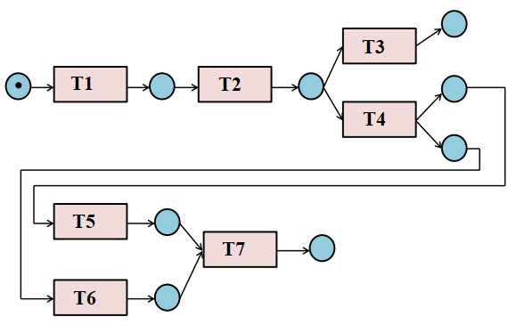
Figure 1: Petri net for the Example Event Log of Table I

Figure 1 depicts a Petri net that conforms to the example event log in Table  I.

Well-known Algorithms for Process Model Discovery

State-of-the-art process discovery techniques include $\alpha$ [10], $\alpha$⁺ [11], Multi-phase miner [12, 13], Heuristics miner [14], Genetic process mining (GPM) [15], $\alpha$⁺⁺ [16], $\alpha$^# [17], $\alpha$^∗ [18], Fuzzy miner [19], Inductive Logic Programming (ILP) [20] algorithms [21]. Other algorithms in the domain of process discovery include Evolutionary tree miner (ETM) [22], Inductive miner [23], Multi-paradigm miner [24]. [25] proposed a hybrid process mining approach that integrates the GPM, particle swarm optimization (PSO), and discrete differential evolution (DE) techniques to extract process models from event logs. [26] proposed the Fodina algorithm, an extension of the Heuristic miner algorithm [26].

[27] proposed an extension of the ETM algorithm [22] that discovers a collection of mutually non-dominating process trees using NSGA-II [28]. This algorithm optimizes replay fitness, precision, generalization, simplicity, and the number of low-level edits.

Motivation for the Proposed Algorithm

Usually, state-of-the-art process discovery algorithms output a single process model that may overfit the training data. To capture the observed behavior more accurately, we propose a multi-objective algorithm for process discovery. The proposed approach yields several candidate solutions. Subsequently, the solutions may either be evaluated by a domain expert to best suit the situation at hand or be chosen by the user based on the local environmental constraints (possibly varying).

The proposed algorithm formulates the problem of process model discovery in a multi-objective framework using the Differential evolution approach [29]. Differential evolution (DE) is a versatile and stable evolutionary algorithm. It evolves individuals through the perturbation of population members with scaled differences of distinct population members. DE algorithm has consistent robust performance and is suitable for solving various numerical optimization problems [30].

Multi-objective Binary Differential Evolution

The proposed algorithm employs a binary version of the differential evolution approach to suit the process mining domain. While DE was initially designed to operate in continuous space, [6] proposed a Binary DE (BDE) algorithm based on dichotomous mutation and crossover operators. The authors [6] verified that compared to other notable BDE variants, the dichotomous BDE improves the diversity of the population and enhances the exploration ability in the binary search space. Also, it has been shown that as compared to other BDE variants, the dichotomous algorithm does not involve any additional computation cost and is faster than other variants of BDE [6].

The past decade has seen the application of the DE approach to problems where the optimization of multiple objectives is required. [31] first proposed a DE-based approach for multi-objective real-coded optimization problems. According to [32], in the case of binary-coded optimization problems, multi-objective BDE algorithms explore the decision space more efficiently than other multi-objective evolutionary algorithms. Subsequently, multi-objective BDE algorithms were also proposed [33], [34], [35], [36], [37].

Materials and Methods

A process discovery algorithm is a function that maps an event log onto a process model that best represents the behavior seen in the event log. In the present work, a process model is represented by a causality relation matrix $C$= ($c_{t_{1},t_{2}}$), where $t_{1},\ t_{2}\ \in[1,n]$ represent the tasks, $c_{t_{1},t_{2}}\in\{0,1\}$, and n is the number of tasks in the given event log. That is, an individual in the population is binary-coded. We, therefore, adapted a binary version of the multi-objective differential evolution algorithm using dichotomous operators [6]. The steps for the proposed multi-objective differential approach for process mining (MoD-ProM) are outlined in Algorithm 9. These steps are explained in the following subsections.

Initialization

The given event log E with n tasks is first consolidated into a dependency measure matrix $D$ indicating the degree of dependencies between tasks [15]. Considering the example in Figure 1, where $T_{1}$, $T_{2}$, $\ldots$, $T_{7}$ represent the tasks. A dependency exists between activities $T_{1}$ and $T_{2}$ if, in a trace, either $T_{1}$ directly precedes $T_{2}$ or vice versa. This is indicated by the presence of either the strings $T_{1}\ T_{2}$ or $T_{2}\ T_{1}$ in a process instance (trace) of the event log. The strength of dependency is proportional to the frequency of occurrence of these strings. In the example log (Figure  1), $T_{1}$ directly precedes $T_{2}$ whereas the string $T_{2}\ T_{1}$ does not occur at all. That is, in the given system, task $T_{1}$ is more likely to be the cause of task $T_{2}$ than vice versa. Dependency measure is computed by counting the length-one-loops (for example, $T_{1}\ T_{2}$), self-loops (for example, $T_{1}\ T_{1}$), length-two-loops (for example, $T_{1}\ T_{2}\ T_{1}$), and parallel tasks (for example, $T_{1}\ T_{2}$ and $T_{2}\ T_{1}$ occur an equal number of times). In the example log (Figure  1), $T_{5}$ and $T_{6}$ are parallel tasks and $T_{1}\ T_{2}$ is a length-one-loop [38].

As proposed by [39], the present work represents a process model as a causality relation matrix. To represent a process model, [39] have favored a causality relation matrix over the more popular Petri net since representing the population individual as a causality relation matrix makes it easier to initialize the population and define the genetic operators. While a causality relation matrix can be directly derived from the information in the event log, in Petri nets, there are places whose existence cannot be derived directly from the event log [39]. The mapping between a Petri net and a causality relation matrix is detailed in [39]. We have graphically depicted both representations for an example event log in Section Process Model Representation titled "Process Model Representation".

Objective Functions and Fitness Evaluation

In the proposed algorithm, we use a novel combination of completeness and generalization as objective functions. Completeness is an important quality dimension because a discovered process model is expected to describe the behavior stored in the log. Completeness is the process of computation of all the parsed tasks while replaying the traces of the log in the model. The missing tokens in a trace and the extra ones left behind during parsing (unconsumed tokens) contribute to the penalty value. Generalization shows whether the process model accurately represents the system as it is and is not "overfitting" to the behavior observed in the event log [40]. Completeness [15] and generalization [41] are computed as in Algorithms 1 and 2 respectively. The algorithms make use of the following function for a given event log E:

$$\raggedleft follows(t_{1},t_{2},E)=\begin{cases}${ 1 if $t_{1}$ $t_{2}$ is length-one-loop in E}$\\ ${ 0, otherwise}$\\ \end{cases}\@add@raggedleft$$ (1)

$$\raggedleft follows_{k}(t_{1},t_{2},E)=\begin{cases}${ 1 if $t_{2}$ is the $k^{th}$ task after $t_{1}$ in E}$\\ ${ 0, otherwise}$\\ \end{cases}\@add@raggedleft$$ (2)

Algorithm 1 Completeness (C, E)

1:n= Total number of tasks/activities in the Event Log E

2:#Traces= Total number of traces in E

3:ParsedTasksRatio =$\frac{1}{n}$ $\sum\limits_{t_{1}=1}^{n}\sum\limits_{t_{2}=1}^{n}c_{t_{1},t_{2}}$ $*follows(t_{1},t_{2},E)$

4:#MissingTokens = $\sum\sum(1-c_{t_{1},t_{2}})$* $follows(t_{1},t_{2},E)$

5:#$Traces_{MissingTokens}$ = $|$traces of MissingTokens$|$

6:#TracesWithoutMissingTokens = #Traces - #$Traces_{MissingTokens}$ + 1

7:#ExtraTokens1 = $\sum\limits_{t_{2}=1}^{n}(\prod\limits_{t_{1}}c_{t_{1},t_{2}})$ where $t_{1}\in[1,n]$ such that $\sum\limits_{t_{2}=1}^{n}c_{t_{1},t_{2}}\geq 1$

8:#ExtraTokens2 =$\sum\limits_{\forall(t_{1},t_{2},t_{3})}[c_{t_{2},t_{3}}*c_{t_{1},t_{3}}*(1-c_{t_{1},t_{2}})*follows(t_{1},t_{2},E)$ ${\ \ \ \ \ \ \ \ \ \ \ \ \ \ \ \ \ \ \ \ \ \ \ \ \ \ \ \ \ \ \ \ \ \ \ \ \ *follows_{k}(t_{1},t_{3},E)*follows_{k-1}(t_{2},t_{3},E)]}$

9:#ExtraTokens= #ExtraTokens1 + #ExtraTokens2

10:#$Traces_{ExtraTokens}$ = $|$traces of ExtraTokens$|$

11:#TracesWithoutExtraTokens = #Traces - $Traces_{ExtraTokens}$ + 1

12:Penalty = $\frac{1}{n}\left[{\dfrac{\#MissingTokens}{\#TracesWithoutMissingTokens}+\dfrac{\#ExtraTokens}{\#TracesWithoutExtraTokens}}\right]$

13:Completeness = ParsedTasksRatio - Penalty

14:Return Completeness

Algorithm 2 Generalization Computation: Generalization (C, E)

1:n= number of tasks/activities in E

2:$executions(t_{1},t_{2})$ = $|(follows(t_{1},t_{2}))|$ * $c_{t_{1},t_{2}}$, $t_{1},\ t_{2}\ \in[1,n]$

3:$executionsFrequency(t_{1})$ = $\sum\limits_{t_{2}=1}^{n}{executions(t_{1},t_{2})}$, $t_{1}\ \in[1,n]$

4:$executionsInvSqrt(t_{1})=\frac{1}{\sqrt{executionsFrequency(t_{1})}}$, $t_{1}\ \in[1,n]$

5:$Generalization=1-\frac{1}{n}{\sum\limits_{t_{1}=1}^{n}{executionsInvSqrt(t_{1})}}$

6:Return Generalization

The present proposal performs an additional analysis of the discovered process models by evaluating their preciseness and simplicity values. The preciseness value of a model is relative to an event log and quantifies the behavior existing in the model but not observed in the event log[42]. A process model with a high precision value is not expected to show behavior not observed in the event log [43]. Completeness and preciseness only consider the relationship between the event log and the process model. However, just a portion of all potential behavior that the system permits is recorded in the event log. Simplicity, instead of telling about the behavior observed in the event log, shows the internal structure of the discovered model. Preciseness [22] and simplicity [44] values are computed as in Algorithms 3 and 4 respectively.

Algorithm 3 Preciseness (C, E)

1:n= number of tasks/activities in E

2:$\#visits(t_{1})$ = $|a_{t_{1}}|$, $a_{t_{1}}$ represent an activity in E, $t_{1}\in[1,n]$

3:$\#outgoingEdges(t_{1})$ = $\sum\limits_{t_{2}=1}^{n}(follows(t_{1},t_{2})>0)$, $t_{1}\in[1,n]$

4:$\#usedEdges(t_{1})$=$\sum\limits_{t_{2}=1}^{n}follows(t_{1},t_{2})*c_{t_{1},t_{2}}$, $t_{1}\in[1,n]$

5:$\#visitedMarkings=\sum\#visits(t_{1})*\frac{\#outgoingEdges(t_{1})-\#usedEdges(t_{1})}{\#outgoingEdges(t_{1})}$

6:$\#totalMarking=\sum\#visits(t_{1})*\#outgoingEdges(t_{1})$

7:$Preciseness=1-\frac{\#visitedMarkings}{\#totalMarking}$

8:Return Preciseness

Algorithm 4 Simplicity (C, E)

1:n= number of tasks/activities in E

2:$sim(t_{1})$ = $\sum\limits_{t_{2}=1}^{n}c_{t_{1},t_{2}}$ + $\sum\limits_{t_{1}=1}^{n}c_{t_{1},t_{2}}$, $t_{1}\in[1,n]$

3:$cardinality=\sum sim(t_{1})$

4:$Simplicity=\frac{1}{cardinality}$

5:Return Simplicity

Constraints and Decision Variables

For a given event log E, Dependency measure matrix $D=(D(t_{1},t_{2}))$ is used to generate causality relation matrices $C^{i}$= ($c_{t_{1},t_{2}}^{i}$) where $i\in[1,N]$ , $t_{1},\ t_{2}\ \in[1,n]$, N is the population size (Algorithm 5). The dependency measure matrix and the causality matrix correspondingly represent the constraints and the decision variables for the problem. Each causality relation matrix represents an individual of the initial population and is computed as [15]:

$$c_{t_{1},t_{2}}^{i}=\begin{cases}${ 1 if r $<$ $D(t_{1},t_{2})$}$\\ ${ 0, otherwise}$\\ \end{cases}$$ (3)

$r\in[0,1)$ is a random number.

Algorithm 5 Computation of initial population of N individuals, each of size n $\times$ n: Initialize Population (n, N, D)

1:for i=1:N do

2:     $C^{i}$=zeros(n,n)

3:     for every tuple $(t_{1},t_{2})$ $\in$ [1, n] $\times$ [1, n] do

4:          Generate a random number r

5:         $c_{t_{1},t_{2}}^{i}\leftarrow$ r $<$ $D(t_{1},t_{2})$

6:     end for

7:end for

8: Return Pop = {$C^{1}$, $C^{2}$, $\ldots$, $C^{N}$}

Mutation

For a population member $C^{i}$= ($c_{t_{1},t_{2}}^{i}$), $i\in[1,N]$ , $t_{1},\ t_{2}\ \in[1,n]$, two other causal matrices $C^{r_{1}}$, $C^{r_{2}}$, $r_{1}$ $\neq$ $r_{2}$ $\neq$ i, $r_{1},r_{2}\ \in[1,N]$ are chosen randomly from the current population. A mutant individual $V^{i}$= ($v_{t_{1},t_{2}}^{i}$) is then created using the following dichotomous mutation scheme [6].

$$\begin{multlined}v_{t_{1},t_{2}}^{i}=((c_{t_{1},t_{2}}^{r_{1}}\oplus c_{t_{1},t_{2}}^{r_{2}})\land rand)\lor(\neg(c_{t_{1},t_{2}}^{r_{1}}\oplus c_{t_{1},t_{2}}^{r_{2}})\land c_{t_{1},t_{2}}^{r_{1}})\end{multlined}v_{t_{1},t_{2}}^{i}=((c_{t_{1},t_{2}}^{r_{1}}\oplus c_{t_{1},t_{2}}^{r_{2}})\land rand)\lor(\neg(c_{t_{1},t_{2}}^{r_{1}}\oplus c_{t_{1},t_{2}}^{r_{2}})\land c_{t_{1},t_{2}}^{r_{1}})$$ (4)

where rand $\in$ $\{0,1\}$, $\land$ denotes the AND operator, $\lor$ denotes the OR operator, $\neg$ denotes the NOT operator, and $\oplus$ denotes the XOR operator. Equation 4 can also be expressed as:

$$v_{t1,t2}^{i}=\begin{cases}${ rand \ if ${c_{t_{1},t_{2}}^{r_{1}}\oplus c_{t_{1},_{t}2}^{r_{2}}}$ $=$ 1}$\\ ${ $c_{t_{1},t_{2}}^{r_{1}}$ \ if ${c_{t_{1},t_{2}}^{r_{1}}\oplus c_{t_{1},t_{2}}^{r_{2}}}$ $=$ 0}$\\ \end{cases}$$ (5)

That is, if $c_{t_{1},t_{2}}^{r_{1}}$ and $c_{t_{1},t_{2}}^{r_{2}}$ are distinct, then the corresponding bit of the mutant individual $v_{t_{1},t_{2}}^{i}$ is randomly chosen as “0” or “1”; otherwise, $v_{t_{1},t_{2}}^{i}$ is set as $c_{t_{1},t_{2}}^{r_{1}}$.

Crossover

The Dichotomous crossover operator [6] starts from the mutant individual $V^{i}$= $v_{t_{1},t_{2}}^{i}$, obtained after application of the dichotomous mutation operator. In this step, the original individual $C^{i}$= ($c_{t_{1},t_{2}}^{i}$) and the mutated individual $V^{i}$ are used to generate a candidate individual $U^{i}$= $u_{t_{1},t_{2}}^{i}$ using the following equation:

$$u_{t_{1},t_{2}}^{i}=\begin{cases}${ $v_{t_{1},t_{2}}^{i}$ if $rand_{t_{1},t_{2}}$ $<$ $CR_{t_{1},t_{2}}$}$\\ ${$c_{t_{1},t_{2}}^{i}$, otherwise}$\\ \end{cases}$$ (6)

where $rand_{t_{1},t_{2}}$ $\in$ [0, 1],

$$CR_{t_{1},t_{2}}=\begin{cases}${ $CR_{1}$ if ($c_{t_{1},t_{2}}^{r_{1}}$ $\oplus$ $c_{t_{1},t_{2}}^{r_{2}}$) $=$ 0 }$\\ ${ $CR_{2}$ if ($c_{t_{1},t_{2}}^{r_{1}}$ $\oplus$ $c_{t_{1},t_{2}}^{r_{2}}$) $=$ 1}$\\ \end{cases}$$ (7)

This operation uses two crossover probabilities $CR_{1}$ and $CR_{2}$ based on dichotomous psychological thinking or "black and white” thinking, with a proclivity for only seeing extremes. After mutation, to generate a candidate individual, if the bits in the randomly chosen individuals from the original population are the same (distinct), then crossover probability $CR_{1}$ ($CR_{2}$) is used. This approach induces diversity in the population and enhances the exploration ability of the proposed approach [6].

Selection

In this section, we outline the selection procedure (Algorithm 6) used to determine the individuals to be preserved from the current population Pop= {$C^{1}$, $C^{2}$,…, $C^{N}$}, and the candidate population $Pop_{U}$= {$U^{1}$, $U^{2}$,…, $U^{N}$} generated after the crossover operation. The process involves identifying the non-dominated individuals.

Algorithm 6 Selection of the fittest individuals from current (Pop) and candidate ($Pop_{U}$) populations, each of size N: Selection ($Pop_{U}$, Pop)

1:for i = 1 to N do

2:     if  $U^{i}$ $\prec$ $C^{i}$   (Equation 8) then

3:         $\texttt{Pop}\leftarrow\textit{($Pop-C^{i}$) $\cup$ $U^{i}$ }$

4:     else if $C^{i}$ $\prec$ $U^{i}$ then

5:         $\texttt{Pop}\leftarrow\textit{Pop}$

6:     else

7:         $\texttt{Pop}\leftarrow\textit{$Pop\cup U^{i}$}$

8:     end if

9:     Return Pop

10:end for

The $i^{th}$ individual from the current population (parent) ($C^{i}$) is said to dominate ($\prec$) the corresponding $i^{th}$ individual in the candidate population (child) ($U^{i}$) if the parent is superior for both the objectives of completeness and generalization, that is,

$$C^{i}\prec U^{i}=\begin{cases}${ 1 \ if $f_{c}(U^{i})\geq f_{c}(C^{i})$ \ \&\&\ $f_{g}(U^{i})\geq f_{g}(C^{i})$ }$\\ ${ 0, otherwise}$\\ \end{cases}$$ (8)

where $f_{c}$ and $f_{g}$ denote the completeness and generalization values respectively.

If the parent (child) dominates the child (parent), then the parent (child) is preserved while the child (parent) is discarded. When neither parent nor child is superior to each other, both the parent and the child are retained.

After eliminating dominated individuals, the number of remaining non-dominated individuals will be between N and 2*N. Since the population size to be carried for the next generation is N, a truncation procedure based on non-dominated sorting (Algorithm 7) and crowding distance (Algorithm 8) is applied [31].

Non-dominated sorting algorithm (Algorithm 7), involves finding rank $1$ individuals of the population that are not dominated by any other individual. Rank $2$ is assigned to those individuals of the population that are dominated by rank $1$ individuals, and so on.

Algorithm 7 Non-Dominated Sorting Algorithm: NonDominatedSorting (Pop, N)

1:for r = 1 to N do

2:     G_r $=$ $\emptyset$ ( Set of individuals dominated by Pop^r)

3:     m_r = 0 (number of individuals that dominate Pop^r)

4:     for s = 1 to N do

5:         if (Pop^r $\prec$Pop^s) (Equation 8)  then

6:              G_r = G_r $\cup$ {Pop^s} (Add Pop^s into G_r)

7:         else if (Pop^s $\prec$ Pop^r)  then

8:              m_r = m_r+1  (increment domination counter m_r)

9:         end if

10:     end for

11:     if m_r= 0 (no solution dominates Pop^r)  then

12:         Front₁= Front₁ $\cup$ {Pop^r} (Pop^r is a member of first front)

13:     end if

14:end for

15:Initialize m_z = $|$G_r$|$

16:k = 1 (initialize front counter)

17:while Front_k $\neq$ $\emptyset$ do

18:     G_z= $\emptyset$ (Store individuals of next front)

19:     for r = 1 to $|$Front_k$|$ do

20:         for z = 1 to $|$G_r$|$ do

21:              m_z = m_z-1 (decrement m_z by one)

22:              if m_z= 0  then

23:                  G_z= G_z $\cup$ {Pop^z}(Pop^z is a member of next front G_z)

24:              end if

25:         end for

26:     end for

27:     k = k+1

28:     Front_k = G_z (Next front is formed with all members of G_z)

29:end while

30:Return Front₁, Front₂,…, Front_N

If the number of non-dominated solutions is greater than the population size N, Euclidean distance is used to truncate individuals from the most crowded region (Algorithm 8). If the rank 1 individuals are less than N, then rank 2 individuals are added, and so on.

Algorithm 8 Pseudo-code for Crowding Distance Algorithm: CrowdingDistance $(C_{s},E)$, $C_{s}$ : Non-dominated solutions

1: l = $|C_{s}|$ // number of non-dominated solutions

2:Initialise the distance vector d= (d₁,d₂,...,d_l)=(0,0,...,0)

3:for j= 1 to l do

4:     Compute $f_{1}^{j}$ = Completeness ($C_{s}^{j}$, E) (Algorithm 1)

5:     Compute $f_{2}^{j}$ = Generalization ($C_{s}^{j}$, E) (Algorithm 2)

6:end for

7:for j= 1 to 2 do

8:     Sort $\{f_{j}^{1},\ldots,f_{j}^{l}\}$ in descending order

9:     d₁ = d_l = $\infty$, // distance associated with best and worst point

10:     for i= 2 to l-1 do

$$d_{i}=d_{i}+\dfrac{|f_{j}^{i+1}-f_{j}^{i-1}|}{|f_{j}^{1}-f_{j}^{l}|}$$

11:     end for

12:end for

13:Remove individual having smallest d value

14:Return Pareto solutions with uniform distribution

Algorithm 9 Pseudo code for Multi-objective Differential Approach for Process Mining (MoD-ProM)

1:Input: N: the population size

2:Read the given event log E, initialize n = #tasks in E

3:Calculate dependency relations (D) between n tasks [15]

4:Pop = Initialize Population (n, N, D) (Algorithm 5) Pop = {$C^{1}$, $C^{2}$, $\ldots$, $C^{N}$}

5:for i= 1 to N do

6:     Compute $f_{C}^{i}$ = Completeness ($C^{i}$, E) (Algorithm 1)

7:     Compute $f_{G}^{i}$ = Generalization ($C^{i}$, E) (Algorithm 2)

8:end for

9:while Stopping criteria (maximum 100 iterations or no improvement for 10 iterations) are not met do

10:     for i = 1 to N  do

11:         Randomly select two other individuals $C^{r_{1}}$, $C^{r_{2}}$, where $r_{1}$ $\neq$ $r_{2}$ $\neq$ i

12:         Generate mutant individual $V^{i}$ using dichotomous mutation operator (Equation 4, 5)

13:         Generate candidate individual $U^{i}$ using dichotomous crossover operator (Equation 6, 7)

14:         Compute completeness & generalization of $U^{i}$

15:     end for

16:     $Pop_{U}$ = $\cup_{i}$ $U^{i}$

17:     Pop= Selection ($Pop_{U}$, Pop) (Algorithm 6)

18:     if Size of (Pop) $>$ N then

19:         $C_{s}$ = NonDominatedSorting (Pop, N) (Algorithm 7)

20:         Pop = CrowdingDistance ($C_{s}$, E) (Algorithm 8)

21:     end if

22:end while

23:Return the Pareto-optimal solutions (Pop)

Results and Discussion

Experimentation

The proposed algorithm is tested on both synthetic and real-world datasets (Table II). Over the last decade, BPI challenge event logs have become important real-world benchmarks in the data-driven research area of process mining. The proposed algorithm is tested for three BPI event logs, namely, BPI 2012 [45], BPI 2013 [46] and BPI 2018 [47], varying in the number of tasks, number of traces, and their domain. BPI 2012 is one of the most studied datasets in process mining. This dataset contains 13,087 traces, and 23 tasks and is derived from a structured real-life loan application procedure released to the community by a Dutch financial institute. The BPI 2013 dataset is from the IT incident management system of Volvo Belgium with 7554 traces and 13 tasks. BPI 2018 covers the handling of applications for EU direct payments for German farmers from the European Agricultural Guarantee Fund. BPI 2018-reference dataset contains 43802 traces and 6 tasks. The proposed algorithm is also tested on a real-life medical event log containing events of sepsis cases from a hospital with 1000 traces and 16 tasks [48]. The proposed algorithm is also run for synthetic logs (ETM, g2-g10 [15, 44, 38]).

The proposed approach is compared with state-of-the-art algorithms, $\alpha$⁺⁺ [16], Heuristic Miner [14], Genetic Miner [15], ILP [20] and Inductive Miner [23] algorithms. For the compared algorithms, the completeness, preciseness, and simplicity values for the synthetic datasets are taken as reported by [44]. However, [44] does not report the value of generalization for these datasets. For the models generated using the Prom tool, $\alpha$⁺⁺, Heuristic Miner, Genetic Miner, and ILP algorithms, the generalization value is computed using the Cobefra tool [49, 44]. We have also compared the proposed strategy with the NSGA-II algorithm for process discovery.

In the proposed multi-objective differential approach for process mining (MoD-ProM), the population size is set to 100, and the value of control parameters $CR_{1}$ and $CR_{2}$ is tuned using grey relational analysis combined with the Taguchi approach (Section Parameter Tuning).

The algorithm is run for a maximum of 100 iterations as the proposed algorithm converges before 100 iterations for most datasets. The total number of runs is fixed at 30.

Table II: Details of Datasets Used in Experiments

Type	Event-log	Tasks	Traces	Events	Source
Synthetic Event logs	ETM	7	100	790	[15, 44]
	g2	22	300	4501
	g3	29	300	14599
	g4	29	300	5975
	g5	20	300	6172
	g6	23	300	5419
	g7	29	300	14451
	g8	30	300	5133
	g9	26	300	5679
	g10	23	300	4117
Real-life Event logs	BPI 2012	23	13087	262200	[45]
	BPI 2013-incident	13	7554	65533	[46]
	BPI 2018-reference	6	43802	128554	[47]
	Sepsis	16	1050	150000	[48]

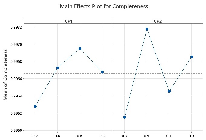
(a)

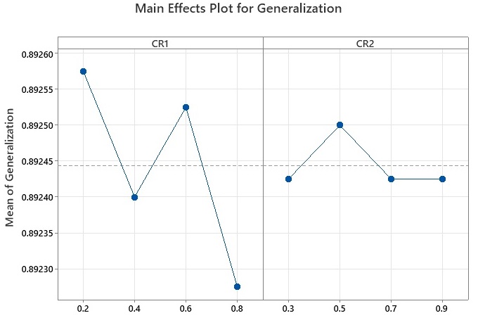
(b)

Figure 2: Main effects plot of Completeness and Generalization

Table III: Experimental results for Completeness and Generalization as per Taguchi L16 Orthogonal Array

RunNo.	Process Parameters		Experimental Results
	CR1	CR2	Completeness	Generalization
1	0.2	0.3	0.9959	0.8931
2	0.2	0.5	0.9996	0.8927
3	0.2	0.7	0.99531	0.8926
4	0.2	0.9	0.9943	0.8919
5	0.4	0.3	0.9945	0.8917
6	0.4	0.5	0.998	0.8928
7	0.4	0.7	0.9971	0.8922
8	0.4	0.9	0.9973	0.8929
9	0.6	0.3	0.9958	0.892
10	0.6	0.5	0.9961	0.893
11	0.6	0.7	0.9994	0.8926
12	0.6	0.9	0.9965	0.8925
13	0.8	0.3	0.9984	0.8929
14	0.8	0.5	0.995	0.8915
15	0.8	0.7	0.994	0.8923
16	0.8	0.9	0.9993	0.8924

Table IV: Grey Relational Generation Values

Run No.	Completeness	Generalization
1	0.339	1.000
2	1.000	0.750
3	0.234	0.687
4	0.054	0.250
5	0.089	0.125
6	0.714	0.813
7	0.554	0.438
8	0.589	0.875
9	0.321	0.313
10	0.375	0.938
11	0.964	0.687
12	0.446	0.625
13	0.786	0.875
14	0.179	0.000
15	0.000	0.500
16	0.946	0.562

Table V: Grey Relational Coefficient and Grey Relational Grade Values

Run No.	Evaluation of $\Delta_{0i}$		Grey relational coefficient		GRG	Rank
	Completeness	Generalization	Completeness	Generalization
Ideal sequence	1	1	1	1
1	0.661	0.000	0.431	1.000	0.715	5
2	0.000	0.250	1.000	0.667	0.833	1
3	0.766	0.313	0.395	0.615	0.505	10
4	0.946	0.750	0.346	0.400	0.373	14
5	0.911	0.875	0.354	0.364	0.359	15
6	0.286	0.187	0.636	0.727	0.682	6
7	0.446	0.562	0.528	0.471	0.499	11
8	0.411	0.125	0.549	0.800	0.675	7
9	0.679	0.687	0.424	0.421	0.423	12
10	0.625	0.062	0.444	0.889	0.667	8
11	0.036	0.313	0.933	0.615	0.774	2
12	0.554	0.375	0.475	0.571	0.523	9
13	0.214	0.125	0.700	0.800	0.750	3
14	0.821	1.000	0.378	0.333	0.356	16
15	1.000	0.500	0.333	0.500	0.417	13
16	0.054	0.438	0.903	0.533	0.718	4

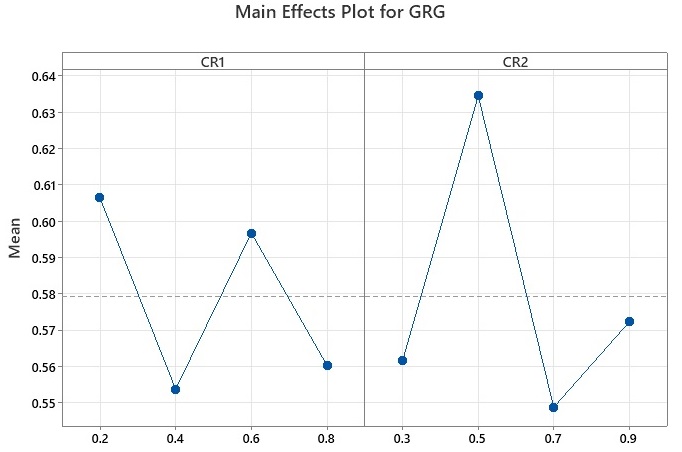
Figure 3: Main effect plot of grey relational grade

Parameter Tuning

To find values of the crossover probabilities, $CR_{1}$ and $CR_{2}$ suitable for the domain of process discovery, the grey relational analysis combined with the Taguchi approach is used [7, 8]. Taguchi method efficiently determines optimal settings of numerous process variables with a minimal set of experiments. Taguchi method suggests replication of the experiment to achieve improved accuracy of the results. Taguchi L16 orthogonal array (OA) design containing 16 experimental runs is used. The results for completeness and generalization are shown in Table III and Figure 2. Dr. Taguchi’s Signal-to-Noise ratios (S$/$N), which are log functions of the desired output, serve as objective functions for optimization [50]. The optimization of numerous performance variables requires a comprehensive assessment of the S/N ratio. The grey relational analysis is used in the study to solve this issue [8].

In the grey relational analysis combined with the Taguchi approach, the experimental data is normalized using Equation 9 to avoid different units and to reduce the variability as presented in Table IV.

$$x^{*}_{i}(k)=\dfrac{x_{i}(k)-min(x_{i}(k))}{max(x_{i}(k))-min(x_{i}(k))}$$ (9)

where, i = 1,…, m; k = 1,…, n, m is the number of experimental data and n is the number of responses. $x_{i}$(k) denotes the original value of $k^{th}$ response for $i^{th}$ experimental run, $x^{*}_{i}$(k) denotes the normalized value after the data pre-processing, max ($x_{i}$(k)) denotes the largest value of $x_{i}$(k), min ($x_{i}$(k)) denotes the smallest value of $x_{i}$(k). The next step is to calculate the grey relational coefficient, $\xi_{i}$(k), from the normalized values by using the following equation (Table V):

$$\xi_{i}(k)=\dfrac{\Delta_{min}-\xi\Delta_{max}}{\Delta_{0i}{k}-\xi\Delta_{max}}$$ (10)

where $\Delta_{0i}$ is the deviation value obtained from the reference value ($x_{0}$(k)) and the comparability value ($x_{i}$(k)).

$$\Delta_{0i}=||x_{0}(k)-x_{i}(k)||$$

$\Delta_{min}$ and $\Delta_{max}$ are the minimum and maximum values of the absolute difference ($\Delta_{0i}$). $\xi$ is the distinguishing coefficient, where $\xi$ $\in$ [0,1] and value 0.5 is used for experimentation [7]. The next step is to find out the grey relational grade (GRG) using the following equation (Table V):

$$\gamma_{i}=\dfrac{1}{n}\sum_{\mathclap{k=1}}^{n}\xi_{i}(k)$$ (11)

where $\gamma_{i}$ is the required grey relational grade for the $i^{th}$ experiment. The results are utilized for optimizing the multi-responses as they are converted to a single grade.

From the value of GRG, the effects of each process parameter at different levels are plotted and shown in Figure 3. Using these results optimal settings for the parameters $CR_{1}$ and $CR_{2}$ are derived as 0.2 and 0.5 respectively.

Table VI: Quality dimensions of non-dominated solutions obtained from MoD-ProM algorithm for synthetic datasets ($f_{C}$: Completeness, $f_{P}$: Preciseness, $f_{S}$: Simplicity, $f_{G}$: Generalization)

ETM				g2				g3				g4				g5
$f_{C}$	$f_{G}$	$f_{S}$	$f_{P}$	$f_{C}$	$f_{G}$	$f_{S}$	$f_{P}$	$f_{C}$	$f_{G}$	$f_{S}$	$f_{P}$	$f_{C}$	$f_{G}$	$f_{S}$	$f_{P}$	$f_{C}$	$f_{G}$	$f_{S}$	$f_{P}$
0.625	0.961	0.967	0.435	0.896	0.946	0.996	0.824	0.818	0.97	1	0.85	0.927	0.969	0.998	0.867	0.916	0.9695	1	0.873
0.813	0.9419	0.984	0.621	0.954	0.934	0.998	0.915	0.906	0.96	1	0.854	0.947	0.957	0.998	0.916	0.946	0.946	1	0.916
0.965	0.911	0.993	0.814	0.972	0.929	0.998	0.941	0.927	0.958	1	0.872	0.948	0.936	0.999	0.944	0.974	0.942	1	0.953
1	0.79	0.994	1	0.988	0.923	0.999	0.979	0.947	0.956	1	0.893	0.96	0.932	1	0.953	1	0.938	1	1
				1	0.916	1	1	0.966	0.953	1	0.915	0.971	0.927	1	0.96
								0.978	0.951	1	0.956	0.982	0.923	1	0.972
								0.99	0.948	1	0.978	0.988	0.917	1	0.984
								1	0.945	1	1	0.994	0.911	1	0.992
												1	0.904	1	1
g6				g7				g8				g9				g10
$f_{C}$	$f_{G}$	$f_{S}$	$f_{P}$	$f_{C}$	$f_{G}$	$f_{S}$	$f_{P}$	$f_{C}$	$f_{G}$	$f_{S}$	$f_{P}$	$f_{C}$	$f_{G}$	$f_{S}$	$f_{P}$	$f_{C}$	$f_{G}$	$f_{S}$	$f_{P}$
0.621	0.9623	1	0.685	0.92	0.979	1	0.902	0.933	0.945	1	0.893	0.842	0.947	1	0.754	0.697	0.938	1	0.767
0.691	0.959	1	0.667	0.947	0.977	1	0.945	0.948	0.935	1	0.932	0.871	0.942	1	0.795	0.787	0.936	1	0.835
0.781	0.951	1	0.743	0.967	0.965	1	0.975	0.96	0.93	1	0.943	0.907	0.939	1	0.83	0.872	0.933	1	0.86
0.844	0.948	1	0.772	0.979	0.963	1	0.981	0.968	0.925	1	0.963	0.937	0.936	1	0.83	0.937	0.932	1	0.799
0.895	0.947	1	0.766	0.989	0.95	1	0.994	0.976	0.919	1	0.983	0.965	0.933	1	0.829	0.959	0.927	1	0.875
0.928	0.943	1	0.798	1	0.947	1	1	0.984	0.914	1	0.987	0.984	0.928	1	0.945	0.976	0.921	1	0.935
0.96	0.94	1	0.906					0.989	0.907	1	0.989	1	0.924	1	1	0.988	0.914	1	0.967
0.973	0.934	1	0.945					0.995	0.9	1	0.993					1	0.907	1	1
0.986	0.929	1	0.993					0.999	0.893	1	1
1	0.923	1	1

Table VII: Quality dimensions of non-dominated solutions obtained by NSGA-II in process mining domain for synthetic datasets ($f_{C}$: Completeness, $f_{P}$: Preciseness, $f_{S}$: Simplicity, $f_{G}$: Generalization)

ETM				g2				g3				g4				g5
$f_{C}$	$f_{G}$	$f_{S}$	$f_{P}$	$f_{C}$	$f_{G}$	$f_{S}$	$f_{P}$	$f_{C}$	$f_{G}$	$f_{S}$	$f_{P}$	$f_{C}$	$f_{G}$	$f_{S}$	$f_{P}$	$f_{C}$	$f_{G}$	$f_{S}$	$f_{P}$
0.505	0.957	0.948	0.371	0.515	0.947	0.987	0.497	0.514	0.969	0.996	0.515	0.48	0.97	0.984	0.372	0.529	0.965	0.986	0.525
0.67	0.942	0.959	0.371	0.775	0.947	0.991	0.671	0.698	0.966	1	0.663	0.532	0.97	0.978	0.396	0.643	0.964	0.992	0.673
0.83	0.927	0.984	0.628	0.858	0.94	0.994	0.786	0.791	0.963	0.998	0.716	0.568	0.969	0.982	0.412	0.755	0.959	0.996	0.753
0.965	0.911	0.993	0.814	0.936	0.933	0.997	0.888	0.863	0.956	1	0.799	0.666	0.963	0.985	0.532	0.809	0.956	0.822	0.796
1	0.79	0.994	1	0.97	0.928	0.998	0.953	0.899	0.956	1	0.845	0.774	0.956	0.992	0.674	0.862	0.953	0.999	0.836
				1	0.916	1	1	0.95	0.952	1	0.862	0.856	0.943	0.994	0.733	0.892	0.949	1	0.879
								0.956	0.949	1	0.87	0.893	0.943	0.996	0.784	1	0.938	1	1
								0.98	0.947	1	0.91	0.915	0.937	0.997	0.857
								0.995	0.945	1	0.966	0.931	0.929	0.998	0.926
g6				g7				g8				g9				g10
$f_{C}$	$f_{G}$	$f_{S}$	$f_{P}$	$f_{C}$	$f_{G}$	$f_{S}$	$f_{P}$	$f_{C}$	$f_{G}$	$f_{S}$	$f_{P}$	$f_{C}$	$f_{G}$	$f_{S}$	$f_{P}$	$f_{C}$	$f_{G}$	$f_{S}$	$f_{P}$
0.654	0.961	0.997	0.504	0.36	0.982	0.989	0.433	0.634	0.949	0.993	0.59	0.565	0.949	1	0.548	0.714	0.931	1	0.583
0.712	0.954	1	0.576	0.464	0.98	0.989	0.468	0.666	0.945	0.994	0.604	0.599	0.948	1	0.641	0.781	0.925	1	0.535
0.765	0.95	1	0.647	0.559	0.979	0.994	0.577	0.792	0.941	0.996	0.677	0.661	0.946	1	0.555	0.868	0.925	1	0.647
0.799	0.946	1	0.72	0.601	0.977	0.992	0.588	0.876	0.939	0.997	0.759	0.693	0.945	1	0.561	0.898	0.922	1	0.647
0.884	0.94	1	0.721	0.698	0.977	0.996	0.678	0.89	0.926	0.998	0.802	0.726	0.943	1	0.643	0.916	0.917	1	0.676
0.926	0.937	1	0.751	0.704	0.974	0.996	0.642	0.912	0.918	0.999	0.819	0.787	0.94	1	0.61	0.917	0.914	1	0.739
0.978	0.928	1	0.831	0.745	0.97	0.996	0.672	0.965	0.903	1	0.92	0.846	0.934	1	0.717	0.942	0.911	1	0.667
0.994	0.923	1	0.871	0.896	0.958	1	0.854	0.989	0.899	1	0.945	0.924	0.929	1	0.754	0.971	0.905	1	0.788
				0.937	0.954	1	0.872	0.995	0.892	1	0.945	0.966	0.927	1	0.787	0.976	0.905	1	0.805
												0.984	0.923	1	0.89

Table VIII: Quality dimensions of non-dominated solutions obtained by NSGA-II for process mining and MoD-ProM algorithm for real-life datasets ($f_{C}$: Completeness, $f_{P}$: Preciseness, $f_{S}$: Simplicity, $f_{G}$: Generalization)

Non-dominated solutions obtained from NSGA-II for process mining algorithm
BPI 2012				BPI 2013				BPI 2018				Sepsis
$f_{C}$	$f_{G}$	$f_{S}$	$f_{P}$	$f_{C}$	$f_{G}$	$f_{S}$	$f_{P}$	$f_{C}$	$f_{G}$	$f_{S}$	$f_{P}$	$f_{C}$	$f_{G}$	$f_{S}$	$f_{P}$
0.794	0.9839	0.9984	0.6945	0.6637	0.9834	0.9964	0.6956	0.9671	0.9857	0.9461	0.406	0.7509	0.9529	0.9955	0.499
0.815	0.9838	0.9986	0.6756	0.8453	0.9758	0.9953	0.6433	0.9873	0.9824	0.9568	0.5989	0.8198	0.9524	0.9958	0.538
0.892	0.9836	0.9987	0.6819	0.9749	0.975	0.997	0.7879	0.9886	0.9792	0.9848	0.7978	0.8872	0.9448	0.9979	0.664
0.899	0.9835	0.9989	0.7151	0.9816	0.9749	0.9971	0.805	0.99	0.979	0.9768	0.7922	0.9033	0.943	0.9974	0.649
0.907	0.9834	0.999	0.6688	0.9832	0.9699	0.9973	0.8308	0.9998	0.9236	0.9907	0.9855	0.9158	0.9345	0.9981	0.704
0.914	0.9832	0.9991	0.6874	0.9871	0.9685	0.9985	0.8818					0.9165	0.931	0.9977	0.670
0.929	0.9831	0.9992	0.7271	0.9916	0.9683	0.9988	0.8915					0.9434	0.9299	0.998	0.714
0.931	0.982	0.9993	0.7056	0.9966	0.9241	0.9983	0.869
				0.9974	0.9239	0.9987	0.8458
Non-dominated solutions obtained from MoD-ProM algorithm
BPI 2012				BPI 2013				BPI 2018				Sepsis
$f_{C}$	$f_{G}$	$f_{S}$	$f_{P}$	$f_{C}$	$f_{G}$	$f_{S}$	$f_{P}$	$f_{C}$	$f_{G}$	$f_{S}$	$f_{P}$	$f_{C}$	$f_{G}$	$f_{S}$	$f_{P}$
0.9146	0.9853	0.9995	0.9229	0.9942	0.9768	0.998	0.7398	0.9965	0.9793	0.985	0.806	0.994	0.961	0.9994	0.849
0.9957	0.985	0.9996	0.9294	0.9946	0.97	0.9979	0.8078	0.9986	0.9792	0.9848	0.7978	0.9957	0.949	0.9995	0.892
0.9965	0.9849	0.9997	0.930	0.9948	0.9696	0.9985	0.8312	0.999	0.979	0.981	0.792	0.9973	0.936	0.9997	0.941
0.9974	0.9828	0.9998	0.9310	0.996	0.9687	0.9989	0.8548	0.9998	0.9236	0.993	0.9858	0.9977	0.908	0.9998	0.972
				0.9961	0.9686	0.999	0.8543
				0.9981	0.9618	0.9996	0.9524
				0.9987	0.9617	0.9994	0.8672
				0.9988	0.9245	0.9995	0.8791

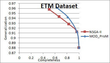
(a)

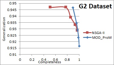
(b)

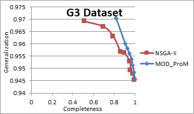
(c)

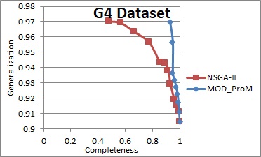
(d)

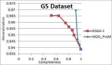
(e)

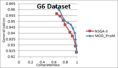
(f)

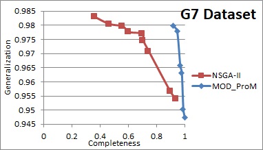
(g)

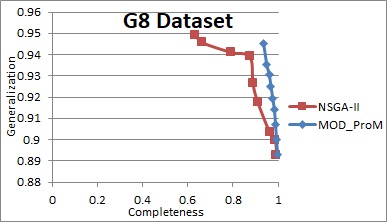
(h)

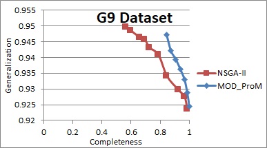
(i)

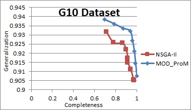
(j)

Figure 4: Pareto-curve for the non-dominated solutions for NSGA-II and MoD-ProM for Synthetic datasets.

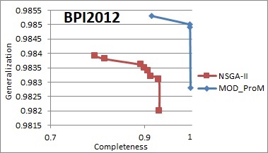
(a)

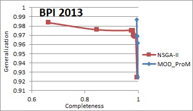
(b)

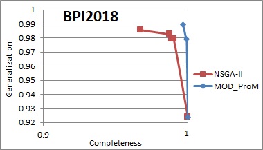
(c)

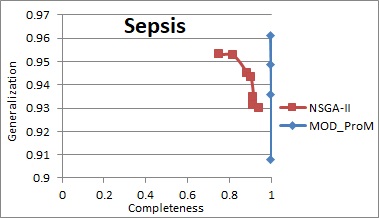
(d)

Figure 5: Pareto-curve for the non-dominated solutions for NSGA-II and MoD-ProM for real-life datasets.

Table IX: Quality dimensions of the models using the state-of-the-art algorithms ($f_{C}$: Completeness, $f_{P}$: Preciseness, $f_{S}$: Simplicity, $f_{G}$: Generalization)

		ETM	g2	g3	g4	g5	g6	g7	g8	g9	g10
Genetic Miner	$f_{C}$	0.3	1	0.31	0.59	1	1	1	0.26	0.48	0.48
	$f_{P}$	0.94	1	0.6	1	1	1	1	0.15	1	1
	$f_{S}$	1	1	1	0.97	1	1	1	0.72	0.96	0.88
	$f_{G}$	0.56	0.91	0.88	0.90	0.921	0.80	0.91	0.88	0.75	0.61
Heuristic Miner	$f_{C}$	0.37	1	1	0.78	1	0.66	1	0.52	0.74	0.78
	$f_{P}$	0.98	1	1	1	1	0.99	1	1	1	1
	$f_{S}$	1	1	1	1	1	0.99	0.98	0.93	0.96	1
	$f_{G}$	0.62	0.913	0.89	0.81	0.92	0.80	0.81	0.90	0.73	0.60
$\alpha$++	$f_{C}$	0.89	0.33	0	1	1	0.45	0	0.35	0.48	0.563
	$f_{P}$	1	0.96	0.18	0.97	1	1	0.12	1	1	1
	$f_{S}$	1	0.78	0.79	1	1	0.76	0.93	0.74	0.79	0.76
	$f_{G}$	0.56	0.62	0.74	0.91	0.92	0.84	0.81	0.91	0.59	0.43
ILP	$f_{C}$	1	1	1	1	1	1	1	1	1	1
	$f_{P}$	1	0.97	0.97	1	1	0.99	1	0.98	0.98	0.95
	$f_{S}$	0.93	0.93	0.92	0.96	1	0.74	0.93	0.667	0.9	0.68
	$f_{G}$	0.79	0.99	0.93	0.91	0.921	0.79	0.91	0.92	0.76	0.61
Inductive Miner	$f_{C}$	0.89	0.958	0.757	0.70	0.80	0.63	0.74	0.79	0.668	0.61
	$f_{P}$	1	0.89	0.73	0.56	0.75	0.41	0.64	0.637	0.423	0.26
	$f_{S}$	1	0.9	0.82	0.81	0.9	0.7	0.85	0.63	0.84	0.65
	$f_{G}$	0.56	0.91	0.94	0.91	0.94	0.91	0.95	0.91	0.88	0.9

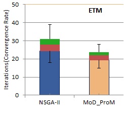
(a)

(b)

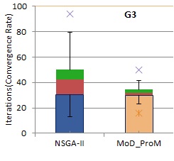
(c)

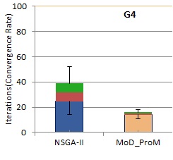
(d)

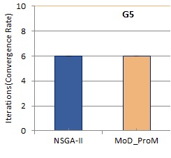
(e)

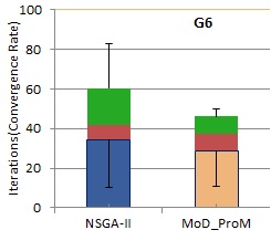
(f)

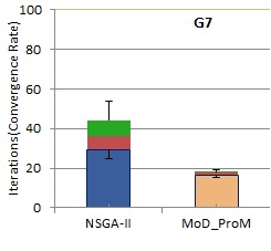
(g)

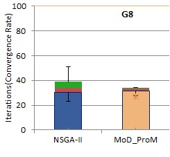
(h)

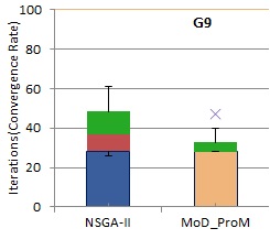
(i)

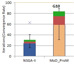
(j)

Figure 6: Convergence rate for NSGA-II and MoD-ProM for synthetic datasets.

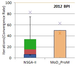
(a)

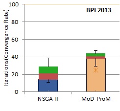
(b)

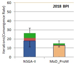
(c)

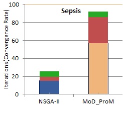
(d)

Figure 7: Convergence rate for NSGA-II and MoD-ProM for real-life datasets.

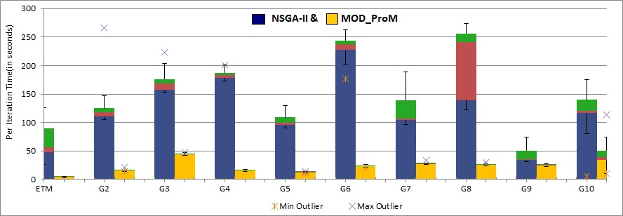
(a) Synthetic Dataset

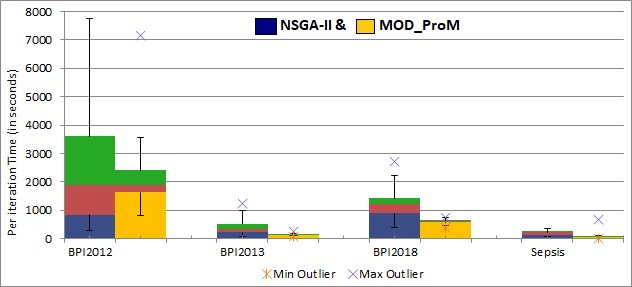
(b) Real-Life Dataset

Figure 8: Comparison of per iteration running time for NSGA-II/MoD-ProM, over 30 runs.

Analysis of the Results

The proposed algorithm (MoD-ProM) is run for the real-life and for the synthetic datasets and the values for quality dimensions, namely completeness ($f_{c}$), preciseness ($f_{p}$), simplicity ($f_{s}$), and generalization ($f_{g}$), for the discovered non-dominated solutions are shown in Tables  VI and  VIII, respectively.

The proposed approach is compared with the NSGA-II algorithm for process discovery. Tables  VII and  VIII present the values for the quality dimensions for the discovered non-dominated solutions for real-life and synthetic datasets, respectively.

Pareto-curves for the non-dominated solutions of NSGA-II and the proposed multi-objective differential evolution for process mining (MoD-ProM) are plotted for comparison (Figure  4 and  5). The Pareto-curves show that in 12 out of 14 datasets, the results of the proposed algorithm are superior to the NSGA-II algorithm.

We also compute the convergence rate and per iteration computation time for NSGA-II and the proposed MoD-ProM, over 30 runs (Figures  6,  7, and  8). While in 2 datasets, the algorithms (NSGA-II, MoD-ProM) show a similar convergence rate, in 8 out of 14 datasets, the proposed MoD-ProM converges faster than NSGA-II, demonstrating superior exploration of the proposed approach. Figure  8 shows that in all cases, the proposed algorithm is superior to NSGA-II in terms of running time per iteration. It is evident from the results that NSGA-II is computationally more expensive than the proposed MoD-ProM algorithm.

The proposed algorithm is also compared with Genetic Miner, Heuristic Miner, $\alpha$⁺⁺, ILP, and Inductive Miner. To rank the proposed approach and the traditional algorithms, additional comparison based on a weighted average [22] of the quality dimensions is made (Table X). [22] proposed a weighted average computation methodology suitable to the process mining domain, as follows:

$$Weighted\ Sum=(10*f_{c}+(1*f_{p})+(1*f_{s})+(1*f_{g}))/13$$ (12)

where for a given process model, $f_{c}$, $f_{p}$, $f_{s}$, and $f_{g}$ denote the completeness, preciseness, simplicity, and generalization values, respectively. A higher weight is assigned to completeness as the process model should be able to reproduce the behavior expressed in the event log.

Table IX shows the quality dimensions for the process model discovered by the state-of-the-art algorithms. The results (Table X) show that the proposed algorithm produces superior-quality process models for all the datasets in terms of the weighted average.

It is also observed that the models generated through the optimization of a combination of completeness and generalization exhibit superior values for the other quality dimensions.

Table X: Weighted sum (Equation 12) of the quality dimensions [22] and the resulting algorithm ranks for each dataset. Rank 7 indicates the best solution

Event Log	Weighted sum							Rank
	GM	HM	$\alpha$++	ILP	Inductive Miner	NSGA-II	MoD-ProM	GM	HM	$\alpha$++	ILP	Inductive Miner	NSGA-II	MoD-ProM
ETM	0.423	0.485	0.881	0.978	0.881	0.983	0.983	1	2	3.5	5	3.5	6.5	6.5
g2	0.993	0.993	0.435	0.991	0.94	0.994	0.994	4.5	4.5	1	3	2	6.5	6.5
g3	0.429	0.991	0.132	0.986	0.77	0.989	0.996	2	6	1	4	3	5	7
g4	0.675	0.816	0.991	0.99	0.71	0.993	0.993	1	3	5	4	2	6.5	6.5
g5	0.994	0.994	0.994	0.994	0.81	0.995	0.995	3.5	3.5	3.5	3.5	1	6.5	6.5
g6	0.984	0.722	0.546	0.963	0.64	0.98	0.994	6	3	1	4	2	5	7
g7	0.993	0.984	0.143	0.988	0.756	0.99	0.996	6	3	1	4	2	5	7
g8	0.334	0.618	0.473	0.966	0.795	0.984	0.992	1	3	2	5	4	6	7
g9	0.578	0.776	0.552	0.972	0.679	0.974	0.994	2	4	1	5	3	6	7
g10	0.561	0.8	0.602	0.941	0.6	0.959	0.993	1	4	3	5	2	6	7

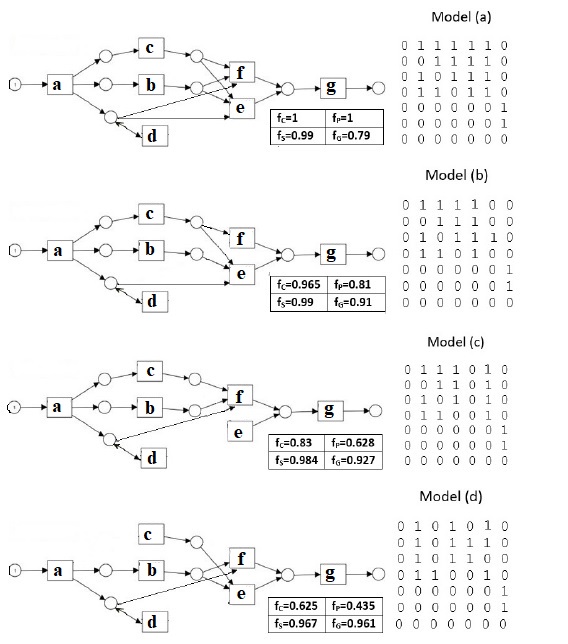
Figure 9: Petri Net and causality relation matrix of non-dominated process models of the proposed algorithm for ETM dataset

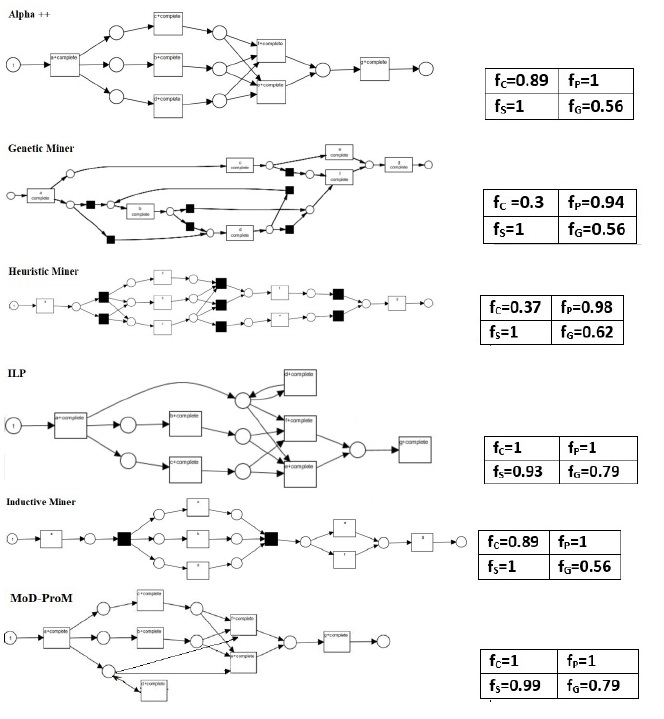
Figure 10: Petri Net of the process models discovered by the compared algorithms for ETM dataset

Process Model Representation

As discussed earlier (Section Initialization on Initialization), the proposed approach represents a process model as a causality relation matrix [39]. However, many state-of-the-art approaches use other semantics, such as Petri net, BPMN models, DFGs, etc. Petri net is possibly the more popular technique for visualizing the discovered process model. We apply the methodology given by [39] to map between a Petri net and a causality relation matrix.

To better explain our results, we have graphically depicted the discovered models (causality relation matrices) as Petri nets for the ETM event log. ETM is a popular dataset in the literature comprising seven tasks. Being a small dataset, it is feasible to show (Figure 9) the causality relation matrices and the corresponding Petri nets of the four models discovered by the proposed algorithm (MoD-ProM).

For the ETM dataset, the ProM tool generated Petri nets for the state-of-the-art algorithms is shown in Figure  10. To compare with the proposed approach, the Petri net of the model with the highest completeness value, discovered by the proposed MoD-ProM, is also drawn in Figure  10.

The completeness or replay fitness [3] quantifies the ability to replay the trace from an event log onto the Petri net [15]. That is, a process model (Petri net) will exhibit a perfect completeness value if every process instance in the given event log can be replayed (simulated) in the Petri net. For the ETM dataset (Figure  10), it is observed that the proposed MoD-ProM algorithm and the ILP algorithm can replay every process instance in the event log. It is observed that the process model discovered by Inductive miner and $\alpha$⁺⁺ do not replay some of the traces, such as (a,b,c,f,g) and (a,c,d,f,g). Traces (a,b,c,d,e,g) and (a,c,b,d,f,g) are not replayed by the model generated by the heuristic miner algorithm. Similarly, the process model generated by the genetic miner algorithm does not replay (a,c,d,b,f,g) and (a,d,c,b,f,g).

Conclusions and Future Works

While conventional process mining algorithms generate a unique process model from the event logs, multi-objective evolutionary algorithms generate several candidate models. The goodness of the generated process models is measured based on quality dimensions such as completeness, generalization, simplicity, and preciseness. A practitioner in the field of process mining may select the most appropriate process model based on the domain requirement. For example, if a user requires a model that replays the maximum number of traces, he/she may pick the model with a better value of completeness [5].

In this paper, we are using the idea of differential evolution towards generating a Pareto-front in the domain of process discovery, a first attempt in this direction. The proposed algorithm performs optimization using completeness and generalization as objective functions. These two quality dimensions make a good pair, as a model with high generalization value can help in improving the current system and can be used for designing future improved processes. Completeness is an important quality dimension because a discovered process model is expected to describe the behavior stored in the log.

The experiments were run for ten synthetic and four real-life datasets, and are repeated 30 times for each dataset. The results are compared with state-of-the-art process discovery algorithms such as $\alpha$⁺⁺, heuristic miner, genetic miner, ILP, and Inductive Miner, and also with NSGA-II for process discovery.

Results show that the models generated by the proposed approach vis-a-vis the compared approaches exhibit a higher value for all the quality dimensions indicating the discovery of “good” process models. The non-dominated solutions generated by the proposed approach (MoD-ProM) are better than those generated by the NSGA-II algorithm for process discovery. The Pareto curve shows that the results of the proposed algorithm are superior or at least as good as that of the NSGA-II algorithm. In terms of computational time requirement, the MoD-ProM algorithm performs consistently better for all datasets as compared to the NSGA-II algorithm.

In summary, we present a novel proposal for process model discovery. The approach employs a multi-objective differential evolution method to optimize the novel combination of completeness and generalization. Results show that the proposed approach is computationally efficient in discovering good-quality process models. However, the proposed approach is limited by the hardware availability.

In the future, we plan to evaluate the applicability of recent multi-objective algorithms [51, 52] in the domain of process discovery and study their computational complexity. In addition, to address the computational intensity and time consumption of process discovery for large event logs, we can explore parallel implementations (multi-core processors, GPU-based processing, and distributed computing environments) for the proposed algorithm.

Data availability

Previously reported data (event logs) were used to support this study and are described in the section Experimentation on Experimentation. These prior studies (and datasets) are cited at relevant places within the text (References [45, 46, 47, 15, 44]).

Conflicts of Interest

The author(s) declare(s) that there is no conflict of interest regarding the publication of this paper.

Funding Statement

This research did not receive any specific grant from funding agencies in public, commercial, or not-for-profit sectors.

References

- [1] Azumah Mamudu, Wasana Bandara, Moe T Wynn and Sander JJ Leemans. “Process mining success factors and their interrelationships”. Business & Information Systems Engineering, pages 1–20, 2024.
- [2] Seyed Mojtaba Hejazi, Mostafa Zandieh and Mirpouya Mirmozaffari. “A multi-objective medical process mining model using event log and causal matrix”. Healthcare Analytics, vol. 3, 100188, 2023. [Online]. Available: https://www.sciencedirect.com/science/article/pii/S2772442523000552.
- [3] Wil MP Van der Aalst. Process mining: data science in action. Springer, 2016.
- [4] Process Mining. “Discovery, conformance and enhancement of business processes”. Springer-Verlag, vol. 8, 18, 2011.
- [5] Sonia Deshmukh, Manoj Agarwal, Shikha Gupta and Naveen Kumar. “Moea for discovering pareto-optimal process models: an experimental comparison”. International Journal of Computational Science and Engineering, vol. 21, no. 3, 446–456, 2020.
- [6] Hu Peng, Zhijian Wu, Peng Shao and Changshou Deng. “Dichotomous binary differential evolution for knapsack problems”. Mathematical Problems in Engineering, vol. 2016, 2016.
- [7] Amlana Panda, A Sahoo and R Rout. “Multi-attribute decision making parametric optimization and modeling in hard turning using ceramic insert through grey relational analysis: A case study”. Decision Science Letters, vol. 5, no. 4, 581–592, 2016.
- [8] CL Lin. “Use of the taguchi method and grey relational analysis to optimize turning operations with multiple performance characteristics”. Materials and manufacturing processes, vol. 19, no. 2, 209–220.
- [9] Kalyanmoy Deb, Amrit Pratap, Sameer Agarwal and TAMT Meyarivan. “A fast and elitist multiobjective genetic algorithm: Nsga-ii”. IEEE transactions on evolutionary computation, vol. 6, no. 2, 182–197, 2002.
- [10] Wil Van der Aalst, Ton Weijters and Laura Maruster. “Workflow mining: Discovering process models from event logs”. IEEE Transactions on Knowledge and Data Engineering, vol. 16, no. 9, 1128–1142, 2004.
- [11] AK Alves de Medeiros, BF Van Dongen, WMP Van Der Aalst and AJMM Weijters. “Process mining: Extending the -algorithm to mine short loops”. Technical report, BETA Working Paper Series, 2004.
- [12] Boudewijn F Van Dongen and Wil MP Van der Aalst. “Multi-phase process mining: Building instance graphs”. In International Conference on Conceptual Modeling, pages 362–376. Springer, 2004.
- [13] Boudewijn F Van Dongen and Wil MP Van der Aalst. “Multi-phase process mining: Aggregating instance graphs into epcs and petri nets”. In PNCWB 2005 workshop, pages 35–58, 2005.
- [14] AJMM Weijters, Wil MP van Der Aalst and AK Alves De Medeiros. “Process mining with the heuristics miner-algorithm”. Technische Universiteit Eindhoven, Tech. Rep. WP, vol. 166, 1–34, 2006.
- [15] Ana Karla Alves de Medeiros. “Genetic process mining”. CIP-DATA LIBRARY TECHNISCHE UNIVERSITEIT EINDHOVEN, printed in, 2006.
- [16] Lijie Wen, Wil MP van der Aalst, Jianmin Wang and Jiaguang Sun. “Mining process models with non-free-choice constructs”. Data Mining and Knowledge Discovery, vol. 15, no. 2, 145–180, 2007.
- [17] Lijie Wen, Jianmin Wang and Jiaguang Sun. “Mining invisible tasks from event logs”. APWeb/WAIM, vol. 4505, 358–365, 2007.
- [18] Jiafei Li, Dayou Liu and Bo Yang. “Process mining: Extending -algorithm to mine duplicate tasks in process logs”. Advances in Web and Network Technologies, and Information Management, pages 396–407, 2007.
- [19] Wil MP Van der Aalst and Christian W Gunther. “Finding structure in unstructured processes: The case for process mining”. In Application of Concurrency to System Design, 2007. ACSD 2007. Seventh International Conference on, pages 3–12. IEEE, 2007.
- [20] Stijn Goedertier, David Martens, Jan Vanthienen and Bart Baesens. “Robust process discovery with artificial negative events”. Journal of Machine Learning Research, vol. 10, no. Jun, 1305–1340, 2009.
- [21] Sonia Deshmukh, Shikha Gupta and Naveen Kumar. “Ga-prom: A genetic algorithm for discovery of complete process models from unbalanced logs”. In International Conference on Big Data Analytics, pages 209–218. Springer, 2021.
- [22] Joos CAM Buijs, Boudewijn F Van Dongen, Wil MP van Der Aalst et al. “On the role of fitness, precision, generalization and simplicity in process discovery.”. In OTM Conferences (1), volume 7565, pages 305–322, 2012.
- [23] Sander JJ Leemans, Dirk Fahland and Wil MP van der Aalst. “Discovering block-structured process models from event logs-a constructive approach”. In International conference on applications and theory of Petri nets and concurrency, pages 311–329. Springer, 2013.
- [24] Johannes De Smedt, Jochen De Weerdt and Jan Vanthienen. “Multi-paradigm process mining: Retrieving better models by combining rules and sequences”. In OTM Confederated International Conferences" On the Move to Meaningful Internet Systems", pages 446–453. Springer, 2014.
- [25] Hsin-Jung Cheng, Chao Ou-Yang and Yeh-Chun Juan. “A hybrid approach to extract business process models with high fitness and precision”. Journal of Industrial and Production Engineering, vol. 32, no. 6, 351–359, 2015.
- [26] Seppe KLM Vanden Broucke and Jochen De Weerdt. “Fodina: A robust and flexible heuristic process discovery technique”. decision support systems, vol. 100, 109–118, 2017.
- [27] Joos CAM Buijs, Boudewijn F van Dongen and Wil MP van der Aalst. “Discovering and navigating a collection of process models using multiple quality dimensions”. In International Conference on Business Process Management, pages 3–14. Springer, 2013.
- [28] Nidamarthi Srinivas and Kalyanmoy Deb. “Muiltiobjective optimization using nondominated sorting in genetic algorithms”. Evolutionary computation, vol. 2, no. 3, 221–248, 1994.
- [29] Rainer Storn and Kenneth Price. “Differential evolution–a simple and efficient heuristic for global optimization over continuous spaces”. Journal of global optimization, vol. 11, no. 4, 341–359, 1997.
- [30] Zhehuang Huang and Yidong Chen. “An improved differential evolution algorithm based on adaptive parameter”. Journal of Control Science and Engineering, vol. 2013, 2013.
- [31] FILIPIcB ROBIcT. “Demo: Differentialevolutionfor multiobjectiveoptimization”. Proceedingsofthe3rd InternationalconferenceonEvolutionaryMulti- criterion Optimization (EMO2005), Guanajuato, Mexico, March 9r11, 2005.
- [32] Tea Tušar and Bogdan Filipič. “Differential evolution versus genetic algorithms in multiobjective optimization”. In International Conference on Evolutionary Multi-Criterion Optimization, pages 257–271. Springer, 2007.
- [33] Yan-Fu Li, Giovanni Sansavini and Enrico Zio. “Non-dominated sorting binary differential evolution for the multi-objective optimization of cascading failures protection in complex networks”. Reliability Engineering & System Safety, vol. 111, 195–205, 2013.
- [34] Bing Xue, Wenlong Fu and Mengjie Zhang. “Differential evolution (de) for multi-objective feature selection in classification”. In Proceedings of the Companion Publication of the 2014 Annual Conference on Genetic and Evolutionary Computation, pages 83–84, 2014.
- [35] Utpal Kumar Sikdar, Asif Ekbal and Sriparna Saha. “Mode: multiobjective differential evolution for feature selection and classifier ensemble”. Soft Computing, vol. 19, no. 12, 3529–3549, 2015.
- [36] Azam Asilian Bidgoli, Hossein Ebrahimpour-Komleh and Shahryar Rahnamayan. “A novel multi-objective binary differential evolution algorithm for multi-label feature selection”. In 2019 IEEE Congress on Evolutionary Computation (CEC), pages 1588–1595. IEEE, 2019.
- [37] Yong Zhang, Dun-wei Gong, Xiao-zhi Gao, Tian Tian and Xiao-yan Sun. “Binary differential evolution with self-learning for multi-objective feature selection”. Information Sciences, vol. 507, 67–85, 2020.
- [38] Shikha Gupta, Sonia Deshmukh and Naveen Kumar. “Mantaray-prom: An efficient process model discovery algorithm”. AI Communications, , no. Preprint, 1–20, 2024.
- [39] Ana Karla A de Medeiros, Anton JMM Weijters and Wil MP van der Aalst. “Genetic process mining: an experimental evaluation”. Data mining and knowledge discovery, vol. 14, 245–304, 2007.
- [40] Joos CAM Buijs, Boudewijn F van Dongen and Wil MP van der Aalst. “Quality dimensions in process discovery: The importance of fitness, precision, generalization and simplicity”. International Journal of Cooperative Information Systems, vol. 23, no. 01, 1440001, 2014.
- [41] ML Van Eck. Alignment-based process model repair and its application to the Evolutionary Tree Miner. PhD thesis, Master’s thesis, Technische Universiteit Eindhoven, 2013.
- [42] Boudewijn F van Dongen, Josep Carmona and Thomas Chatain. “A unified approach for measuring precision and generalization based on anti-alignments”. In Business Process Management: 14th International Conference, BPM 2016, Rio de Janeiro, Brazil, September 18-22, 2016. Proceedings 14, pages 39–56. Springer, 2016.
- [43] Felix Mannhardt, Massimiliano De Leoni, Hajo A Reijers and Wil MP Van Der Aalst. “Measuring the precision of multi-perspective process models”. In Business Process Management Workshops: BPM 2015, 13th International Workshops, Innsbruck, Austria, August 31–September 3, 2015, Revised Papers 13, pages 113–125. Springer, 2016.
- [44] Borja Vázquez-Barreiros, Manuel Mucientes and Manuel Lama. “Prodigen: Mining complete, precise and minimal structure process models with a genetic algorithm”. Information Sciences, vol. 294, 315–333, 2015.
- [45] BF Van Dongen and BPI Challenge. “Event log of a loan application process”. Eindhoven University of Technology, 2012. [Online]. Available: https://data.4tu.nl/articles/dataset/BPI_Challenge_2012/12689204.
- [46] Ward Steeman. “Bpi challenge 2013, incidents”. 2013. [Online]. Available: https://doi.org/10.4121/uuid:500573e6-accc-4b0c-9576-aa5468b10cee.
- [47] Boudewijn Van Dongen and F. (Florian) Borchert. “Bpi challenge 2018”, Mar 2018. [Online]. Available: https://data.4tu.nl/articles/dataset/BPI_Challenge_2018/12688355/1.
- [48] F Mannhardt. “Sepsis cases–event log (2016)”, 2016. [Online]. Available: https://data.4tu.nl/articles/dataset/Sepsis_Cases_-_Event_Log/12707639.
- [49] Seppe KLM Vanden Broucke, Jochen De Weerdt, Jan Vanthienen and Bart Baesens. “A comprehensive benchmarking framework (cobefra) for conformance analysis between procedural process models and event logs in prom”. In 2013 IEEE Symposium on Computational Intelligence and Data Mining (CIDM), pages 254–261. IEEE, 2013.
- [50] Alessandro Freddi and Mario Salmon. “Introduction to the taguchi method”. In Design principles and methodologies, pages 159–180. Springer, 2019.
- [51] Bilal H Abed-alguni and Saqer Hamzeh AL-Jarah. “Ibja: An improved binary djaya algorithm for feature selection”. Journal of Computational Science, vol. 75, 102201, 2024.
- [52] Noor Aldeen Alawad, Bilal H Abed-alguni, Mohammed Azmi Al-Betar and Ameera Jaradat. “Binary improved white shark algorithm for intrusion detection systems”. Neural Computing and Applications, vol. 35, no. 26, 19427–19451, 2023.