Physics-Informed AI Inverter

Abstract

This letter devises an AI-Inverter that pilots the use of a physics-informed neural network (PINN) to enable AI-based electromagnetic transient simulations (EMT) of grid-forming inverters. The contributions are threefold: (1) A PINN-enabled AI-Inverter is formulated; (2) An enhanced learning strategy, balanced-adaptive PINN, is devised; (3) extensive validations and comparative analysis of the accuracy and efficiency of AI-Inverter are made to show its superiority over the classical electromagnetic transient programs (EMTP).

I Introduction

Three-phase inverter plays a fundamental role in the modern power grid. Over the past decades, various modeling techniques, such as the PWM switch model, and state-space averaged model, have been pivotal for inverters [1, 2]. The emphasis on model-based analytics has underscored the need for further developments in the modeling of power inverters [3]. However, in real-life scenarios, the actual inverter which undergoes noise and nolinearity, does not faithfully function as the detailed model with static parameters. A machine learning-based model, trained using measurements and integrating underlying physical principles, can better replicate real-world operations and adapt as it encounters various scenarios. This learning-based model acts as a lightweight digital twin of the original system, providing enhanced accuracy compared to the detailed static model.

This intuition naturally leads to Physics-Informed Neural Networks (PINN). Dislike traditional data-driven modeling which requires acquiring high-quality real-time data sets, PINNs efficiently address the limitations of data availability and compromised generalization ability by incorporating the governing physics into the training. In PINN, a persistent challenge emerges in the formulation of an effective loss function. Unlike conventional data-driven training, the loss function in PINN often involves multiple terms [4]. Determining how to allocate the weights for each term in the loss function has been an open problem. Therefore, there is a pressing need for a lightweight yet efficient structure when modeling inverters.

II Physical formulation of an inverter

Inverters interface and transfer energy between DC and AC subsystems. Fig. 2 shows the structure of a grid-forming inverter where the purple box represents the control block.

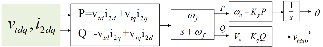
Figure 1: Power controller.

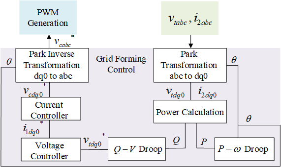
Figure 2: Block diagram of the grid forming control structure.

The power calculation, $P-\omega$ droop and $Q-V$ droop control in Fig. 2 consist of the power controller, which is detailed below:

$$P=v_{td}i_{2d}+v_{tq}i_{2q}, ~{}Q=-v_{td}i_{2q}+v_{tq}i_{2d}$$ (1)

$$\omega=\omega_{n}-k_{p}\cdot P\cdot\frac{\omega_{f}}{s+\omega_{f}}, ~{}V=V_{n}-k_{q}\cdot Q\cdot\frac{\omega_{f}}{s+\omega_{f}}$$

The voltage controller in Fig. 2 can be represented as:

$$v_{td}^{*}=V ,~{}v_{tq}*=0$$ (2)

$$\frac{d\phi_{d}}{dt}=v_{td}^{*}-v_{td} ,~{}\frac{d\phi_{q}}{dt}=v_{tq}^{*}-v_{tq}$$

$$i_{1d}^{*}=Fi_{2d}-\omega_{n}C_{f}v_{tq} +K_{pv}\cdot(v_{td}^{*}-v_{td})+K_{iv}\phi_{d}$$

$$i_{1q}^{*}=Fi_{2q}-\omega_{n}C_{f}v_{td} +K_{pv}\cdot(v_{tq}^{*}-v_{tq})+K_{iv}\phi_{q}$$

The current controller is:

$$\frac{d\gamma_{d}}{dt}=i_{1d}^{*}-i_{1d} ,~{}\frac{d\gamma_{q}}{dt}=i_{1q}^{*}-i_{1q}$$ (3)

$$v_{cd}^{*}=-\omega_{n}\cdot L\cdot i_{1q} +K_{pc}\cdot(i_{1d}^{*}-i_{1d})+K_{ic}\gamma_{d}$$

$$v_{cq}^{*}=\omega_{n}\cdot L\cdot i_{1d} +K_{pc}\cdot(i_{1q}^{*}-i_{1q})+K_{ic}\gamma_{q}$$

Collecting all the equations from the power, voltage and current controllers, an inverter can be formulated as [5]:

$$\frac{dx}{dt} =Ax+Bu+const$$ (4)

$$v =Cx+D\tilde{u}$$

where $v_{c,qd0}$ is denoted as $v$ for brevity, $x=[\omega,V,\theta,\phi_{d},\phi_{q},\gamma_{d},\gamma_{q}]^{T}$, $\tilde{u}=[v_{td},v_{tq},i_{2d},i_{2q},i_{1d},i_{1q}]^{T}$, $u=[P,Q,\tilde{u}^{T}]^{T}$.

III Physics-informed AI-Inverter

III-A Physics-informed learning for inverter

Define a neural network $\mathcal{N}$ that is capable of predicting $\hat{v}$ with inputs of $\tilde{u}$ and $t$. Here ^$\wedge$ denotes the predicted values from $\mathcal{N}$. Then the final output $\hat{v}_{c,abc}$ can be calculated via inverse Park transformation, here $\hat{\theta}$ is one of the state variables within $\hat{x}$:

$$\hat{v},\hat{x}=\mathcal{N}(\tilde{u},t)$$ (5)

$$\hat{v}_{c,abc}=InvPark(\hat{v},\hat{\theta})$$

The core idea of physics-informed learning for AI-Inverter is to integrate the physical equations (4) in the loss function of training, ensuring the predicted values in (5) satisfy the physical constraints. Therefore, the loss function can be formulated into a physical term and a data-driven term:

$$\mathcal{L} =L_{phy}+L_{data}$$ (6)

For the data-driven term $L_{data}$, define:

$$L_{data}=||\hat{v}-{v}||_{2}+||\hat{x}-{x}||_{2}$$ (7)

Then derive the physics-informed loss function based on the numerical integration of (4). Without loss of generality, an estimation of $\hat{x}$ is performed by the modified Euler rule:

$$\hat{x}^{\prime}(t+\Delta t)=\frac{\Delta t}{2}[\frac{d\hat{x}(t+\Delta t)}{dt}+\frac{d\hat{x}(t)}{dt}]+\hat{x}(t)$$ (8)

$$s.t. ~{}\frac{d\hat{x}(t+\Delta t)}{dt}=A\hat{x}(t+\Delta t)+Bu(t+\Delta t)+const$$

where $d\hat{x}(t+\Delta t)/{dt}$ is an estimation of the derivative of $\hat{x}$ at time $t+\Delta t$. It is calculated using the predicted value $\hat{x}$ from the neural network. $\Delta t$ is the time step. The loss function for $L_{dx}$ is developed as:

$$L_{dx}=mean||\Delta dx||_{2}$$ (9)

$$s.t. ~{}\Delta dx(t)=\hat{x}^{\prime}(t+\Delta t)-\hat{x}(t+\Delta t)$$

Similarly, define $L_{v}$ and $L_{Cx}$ as:

$$L_{v}=mean||\Delta\hat{v}||_{2},~{}L_{Cx}=mean||\Delta{Cx}||_{2}$$ (10)

$$s.t. ~{}\Delta\hat{v}=\widehat{Cx}+D\tilde{u}-\hat{v},~{}\Delta Cx=C\cdot\hat{x}-\widehat{Cx}$$

$\widehat{Cx}$ is an intermediate regularizing term predicted by the NN, thereby improving accuracy.

The physical term $L_{phy}$, comprising $L_{v}$ and $L_{dx}$, $L_{Cx}$, quantifies the discrepancy between the predicted values from the neural network and the values calculated using the physical equations in (4). The structure of the physics-informed AI-Inverter is illustrated in Fig. 3.

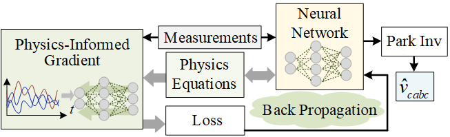
Figure 3: Schematic diagram of physics-informed AI-Inverter

III-B Balanced-adaptive physics-informed AI-Inverter

An effective loss function is critical to the efficiency and accuracy of a PINN. To start, the ranges of $L_{v}$, $L_{dx}$, and $L_{Cx}$ differ, each reflecting distinct physical meanings. Additionally, multiple terms contribute to $\mathcal{L}$. Hence, we propose a balanced and adaptive physics-informed loss function as shown in Fig. 4, which aims to mitigate the disproportionate influence of individual terms and automatically assign weights to each term by:

$${\cal L} =\frac{\lambda_{a}L_{v}+\lambda_{b}L_{dx}+\lambda_{c}L_{Cx}}{\max(L_{v},L_{dx},L_{Cx})}$$ (11)

$$\mathop{\min}\limits_{\theta}\mathop{\max}\limits_{{\lambda_{a}},{\lambda_{b}},{\lambda_{c}}}{\cal L}(\theta,{\lambda_{a}},{\lambda_{b}},{\lambda_{c}})$$

The loss is optimized in a self-supervised manner that ascends in the loss weight space and descends in the model parameter space:

$$\theta^{*}\leftarrow\theta-\frac{\partial\mathcal{L}}{\partial\theta},~{}~{}\lambda^{*}\leftarrow\lambda+\frac{\partial\mathcal{L}}{\partial\lambda}$$ (12)

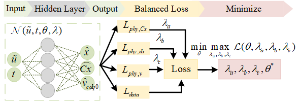
Figure 4: Structure of balanced-adaptive AI-Inverter

IV Case Study

This section presents case studies performed on the IEEE 39 bus system, focusing on the integration of an AI-Inverter, as illustrated in Fig. 5. The primary goal is to maximize the utilization of limited data, with training sets comprising only 6 scenarios. Despite this, the testing phase involved 20 different cases, including various fault occurrences and durations, represented by the open switch in Fig. 5, and random load changes ranging from 0.8 to 1.2 times the original load.

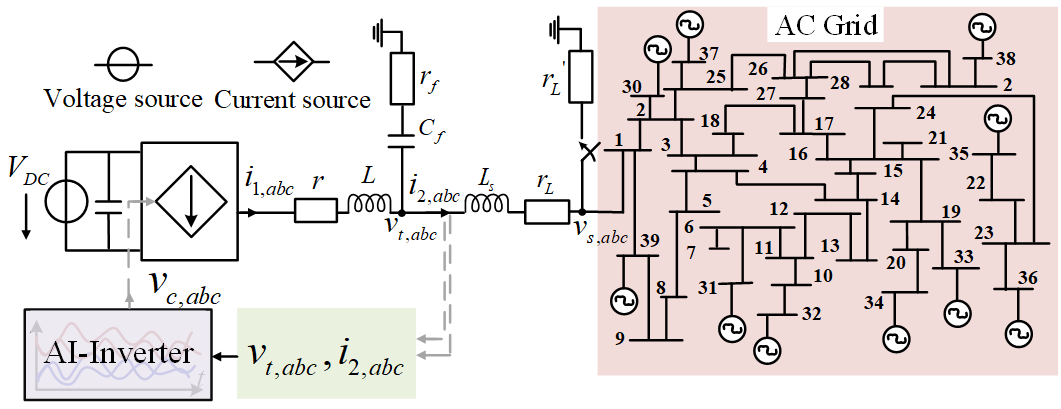
Figure 5: Interface of AI-Inverter with IEEE 39 bus system.

TABLE I: Parameters for inverter

Parameter	Value
$\omega_{n}$, $\omega_{f}$, $F$,$V_{n}$	2$\pi$*60 ($f$=60 Hz), 10$\pi$, 0.75, 230Kv
$r$, $r_{L}$, $r_{s}$, L, $L_{s}$	0.1, 16, 0.3, 1.35e-3, 0.35e-3
$K_{p}$, $K_{q}$,$K_{pc}$	9.4e-5, 1.3e-4, 31.5
$K_{ic}$, $K_{pv}$, $K_{iv}$	8e4, 0.2, 3120

Training sets were simulated using a detailed full-order physical model in Python 3.7, cross-validated with RTDS results. The neural network adopts a multilayer perceptron structure with 2 hidden layers containing [128,64] neurons. Key parameters are summarized in Table I.

IV-A Efficacy of AI-Inverter under varied operational conditions

The dynamic simulation of the system requires assembling the neural AI-Inverter with the rest of the physics model, referred to as closed-loop simulation. In this process, the AI-Inverter is incorporated back into the system in a step-by-step simulation. Therefore, the accuracy of the neural network outputs directly influences the results for the subsequent timestep.

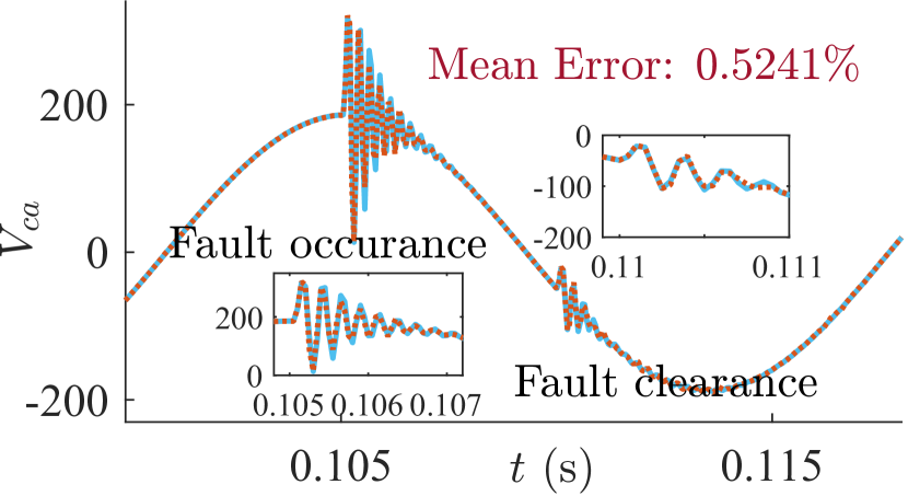
(a) Predicted $V_{a}$ under fault

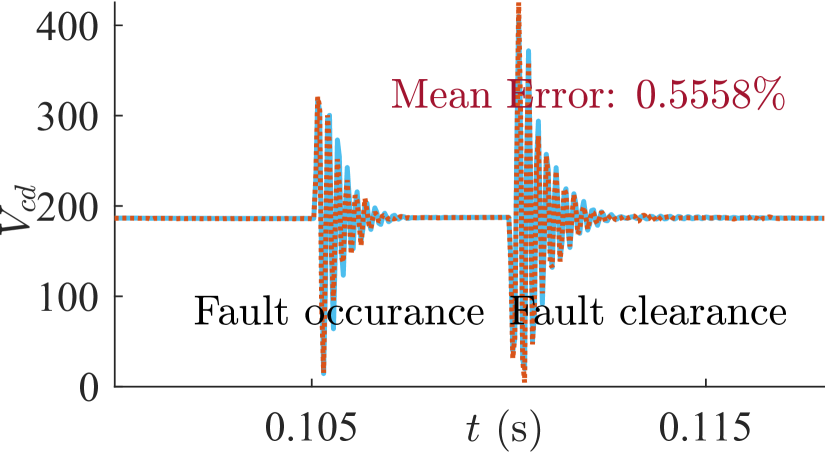
(b) Predicted $V_{d}$ under fault

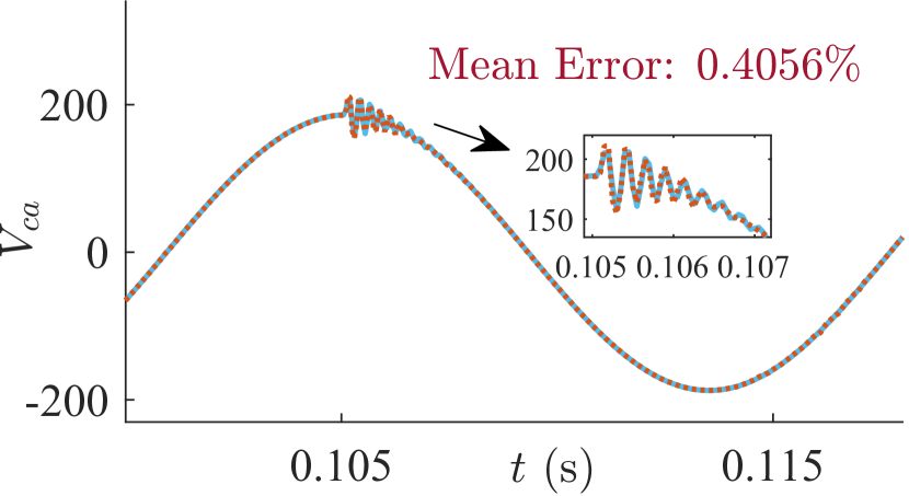
(c) Predicted $V_{a}$ under load change

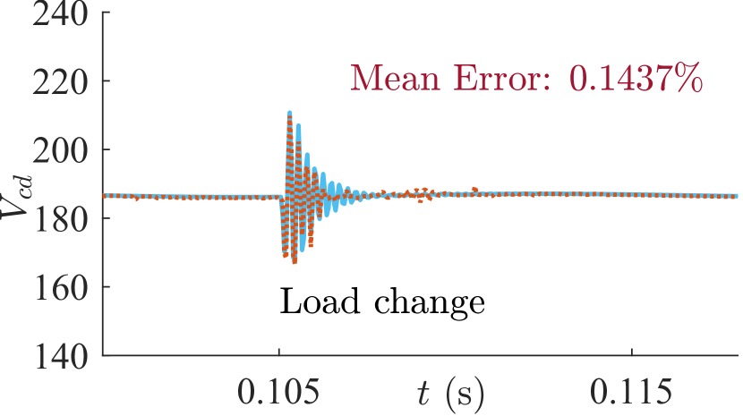
(d) Predicted $V_{d}$ under load change

Figure 6: Predictions of voltages of AI-Inverter under fault and load change.

Fig. 6 presents the closed-loop performance of the AI-Inverter, showing the high accuracy of predictions under fault and load change respectively.

Fig. 7 shows the time-series relative error of predictions across 20 scenarios. The results demonstrate that, even under unforeseen circumstances, the AI-Inverter maintains reasonable error rates throughout the time horizon. It can preserve dynamic behaviors following contingencies not included in the training datasets.

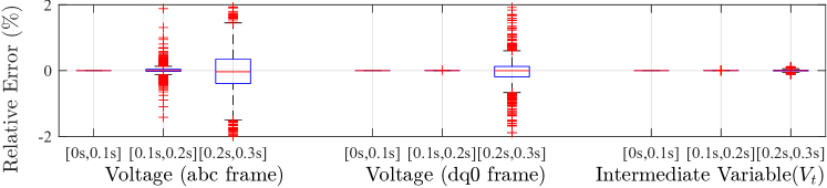
Figure 7: Error rate of voltages under 20 fault cases.

IV-B Comparative analysis

This subsection evaluates the proposed balanced-adaptive PINN (BA-PINN) against existing purely data-driven methods and a baseline PINN. Figure 8 shows that all three approaches use the same neural network structure and training datasets under a fault scenario. As illustrated in Fig. 8(a), each method achieves satisfactory results during open-loop training, indicating successful network convergence. However, during the closed-loop test presented in Fig. 8(b), the baseline PINN displays irregular oscillations, and the data-driven method fails to converge by the end of the trajectory.

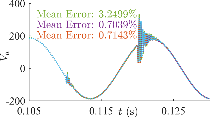
(a) Open-loop training of $V_{a}$

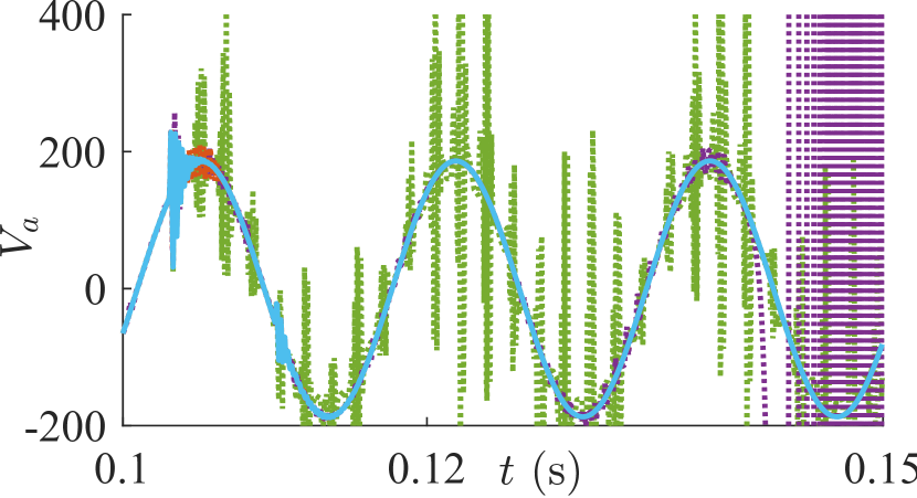
(b) Closed-loop testing of $V_{a}$

Figure 8: Comparison of performances via different methods

This discrepancy occurs because, during the closed-loop test, the neural network interacts with the physical system at each time step, causing even minor residual errors to accumulate over time. As depicted in Fig. 8(a) and detailed in Table II, the baseline PINN encounters slight difficulties during open-loop training, requiring more iterations to achieve satisfactory results. Its poor performance in the closed-loop test reveals suboptimal network behavior. The data-driven method’s sensitivity to both the quantity and quality of data renders it unstable when faced with unexpected data.

TABLE II: MSE comparsion

Method	Data-driven	Baseline PINN	BA-PINN
Error Rate	65.9169%	17.8807%	0.6015%
Training iterations	4100	6000	4100
MSE	1.7914e3	76.2240	4.1921

V Conclusion

This letter introduces a physics-informed AI-Inverter, leveraging physical equations and optimizing automatically in a balanced adaptive manner. It eliminates the need for extensive EMTP trajectories as training samples. When integrated into a connected system, the AI-Inverter demonstrates efficacy under various contingencies, surpassing purely data-driven methods and baseline PINNs in performance.

References

- [1] R. W. Erickson and D. Maksimovic, Fundamentals of power electronics. Springer Science & Business Media, 2007.
- [2] R. D. Middlebrook and S. Cuk, “A general unified approach to modelling switching-converter power stages,” in 1976 IEEE power electronics specialists conference, pp. 18–34, IEEE, 1976.
- [3] S. Vazquez, J. I. Leon, L. G. Franquelo, J. Rodriguez, H. A. Young, A. Marquez, and P. Zanchetta, “Model predictive control: A review of its applications in power electronics,” IEEE industrial electronics magazine, vol. 8, no. 1, pp. 16–31, 2014.
- [4] S. Subramanian, R. M. Kirby, M. W. Mahoney, and A. Gholami, “Adaptive self-supervision algorithms for physics-informed neural networks,” arXiv preprint arXiv:2207.04084, 2022.
- [5] N. Pogaku, M. Prodanovic, and T. C. Green, “Modeling, analysis and testing of autonomous operation of an inverter-based microgrid,” IEEE Transactions on Power Electronics, vol. 22, no. 2, pp. 613–625, 2007.