Grass: Compute Efficient Low-Memory LLM Training with Structured Sparse Gradients

Abstract

Large language model (LLM) training and finetuning are often bottlenecked by limited GPU memory. While existing projection-based optimization methods address this by projecting gradients into a lower-dimensional subspace to reduce optimizer state memory, they typically rely on dense projection matrices, which can introduce computational and memory overheads. In this work, we propose Grass (GRAdient Stuctured Sparsification), a novel approach that leverages sparse projections to transform gradients into structured sparse updates. This design not only significantly reduces memory usage for optimizer states but also minimizes gradient memory footprint, computation, and communication costs, leading to substantial throughput improvements. Extensive experiments on pretraining and finetuning tasks demonstrate that Grass achieves competitive performance to full-rank training and existing projection-based methods. Notably, Grass enables half-precision pretraining of a 13B parameter LLaMA model on a single 40GB A100 GPU—a feat infeasible for previous methods—and yields up to a $2\times$ throughput improvement on an 8-GPU system. Code can be found at https://github.com/aashiqmuhamed/GRASS.

Grass: Compute Efficient Low-Memory LLM Training with Structured Sparse Gradients

Aashiq Muhamed¹, Oscar Li², David Woodruff³, Mona Diab¹, Virginia Smith² {amuhamed, runlianl, dwoodruf, mdiab, smithv}@andrew.cmu.edu ¹ Language Technologies Institute, ² Machine Learning Department ³ Department of Computer Science Carnegie Mellon University

1 Introduction

Pretraining and finetuning large language models (LLMs) are often memory bottlenecked: storing model parameters, activations, gradients, and optimizer states in GPU memory is prohibitively expensive. As an example, pretraining a LLaMA-13B model from scratch under full bfloat16 precision with a token batch size of 256 requires at least 102 GB memory (24GB for trainable parameters, 49GB for Adam optimizer states, 24GB for weight gradients, and 2GB for activations), making training infeasible even on professional-grade GPUs such as Nvidia A100 with 80GB memory (Choquette et al., 2021). Existing memory efficient system-level techniques like DeepSpeed optimizer sharding/offloading (Rajbhandari et al., 2020) and gradient checkpointing (Chen et al., 2016) trade off throughput for memory advantages which slow down pretraining. As models scale, the memory and compute demands of increasingly large LLMs continue to outpace hardware advancements, highlighting the need for advances in optimization algorithms beyond system-level techniques.

Various optimization techniques have been proposed to enhance the efficiency of LLM training. One prominent approach is parameter-efficient finetuning (PEFT), such as Low-Rank Adaptation (LoRA), which reparameterizes weight matrices using low-rank adaptors (Hu et al., 2021). This significantly reduces the number of trainable parameters, yielding smaller optimizer states and gradients. However, despite its efficiency, LoRA and its derivatives (Sheng et al., 2023; Zhang et al., 2023; Xia et al., 2024) often underperform compared to full-rank finetuning (Biderman et al., 2024). Variants like ReLoRA (Lialin et al., 2023) extend LoRA to pretraining by periodically updating the full matrix with new low-rank updates, but it still requires a costly initial full-rank training warmup which makes it impractical in memory-constrained scenarios.

Algorithm 1 Memory-efficient Subspace Optimization

1:Initial weights $W_{0}\in\mathbb{R}^{m\times n}$ with $m\leq n$; update frequency $K$; total iterations $T$; subspace rank $r$ with $r\ll m$, an off-the-shelf optimizer opt; function to update the optimizer state, scale factor $\alpha$.

2:Optimized weights $W^{(T)}$

3:$t\leftarrow 0$

4:$W^{(0)}\leftarrow W_{0}$ $\triangleright$ Set initial weights $W_{0}\in\mathbb{R}^{m\times n}$

5:$S^{(0)}\leftarrow\texttt{opt.init}(0^{r\times n})$ $\triangleright$ Adam state $\in\mathbb{R}^{2\times r\times n}$

6:while $t\leq T$ do

7:     if $t\equiv 0\pmod{K}$ then

8:         // Compute new projection matrix

9:         $P\leftarrow$ $\triangleright$ $P\in\mathbb{R}^{m\times r}$

10:         // [Optional] Update optimizer state

11:         $S^{(t)}\leftarrow$

12:     end if

13:     $G_{C}\leftarrow$ $\triangleright$ $G_{C}\in\mathbb{R}^{r\times n}$

14:     $S^{(t+1)},\Delta^{(t+1)}\leftarrow\texttt{opt.update}(S^{(t)},G_{C})$

15:     $W^{(t+1)}\leftarrow$ $\triangleright$ Apply update

16:     $t\leftarrow t+1$

17:end while

To allow for full-rank pretraining and finetuning, another approach for memory-efficient LLM training involves designing adaptive optimizers (Shazeer and Stern, 2018). One such class, memory-efficient subspace optimizers, utilizes projection matrices ($P$) to project high-dimensional gradients into a lower-dimensional space and performs optimization within the subspace. This projection significantly reduces the memory footprint required to store optimizer states. Existing methods such as GaLore (Zhao et al., 2024) and Flora (Hao et al., 2024) employ dense projection matrices, which introduce additional memory and computational overhead. In contrast, we employ structured sparse matrices for $P$, demonstrating their advantages in memory, computation, and communication efficiency across both pretraining and finetuning. Our main contributions include:

1. We introduce Grass, a novel method that enables full parameter training of LLMs with structured sparse gradients. By leveraging sparse projection matrices, Grass significantly reduces memory consumption and communication overhead compared to existing projection-based optimization techniques. We theoretically motivate and empirically analyze effective ways to construct the sparse projection matrix for Grass.

2. We conduct extensive experiments on both pretraining and finetuning tasks, demonstrating that Grass converges faster in wall-clock time than existing projection-based methods due to its additional compute efficiency benefits. Grass exhibits minimal performance degradation (<0.1 perplexity gap) compared to full-rank training on the 1B parameter LLaMA model while achieving a 2.5$\times$ reduction in memory footprint.

3. We present an optimized PyTorch implementation of Grass for modern hardware, incorporating implementation tricks to enhance training throughput, stability, and scalability. For pretraining a 1B LLaMA model, Grass achieves a 25% throughput increase on a single GPU and up to a 2$\times$ throughput improvement on 8 GPUs over full-rank training and GaLore. Furthermore, Grass’s low memory footprint enables half-precision training of a 13B LLaMA model on a single 40GB A100 GPU, a feat that existing projection-based optimization methods cannot achieve.

2 A Unified View of Memory-efficient Subspace Optimizers (MeSO)

High memory usage of full-rank training.

Standard full-rank training of the weight matrix $W\in\mathbb{R}^{m\times n}$ in any linear layer of an LLM involves 1) computing the full-parameter gradient $G_{W}\coloneqq\nabla L(W)$ and 2) using it to update the model weights and optimizer states:

$$S^{(t+1)},\Delta W^{(t)}\leftarrow \;\texttt{opt.update}(S^{(t)},\nabla L(W^{(t)}))$$

$$W^{(t+1)}\leftarrow \;W^{(t)}+\Delta W^{(t)}$$ (1)

Here, opt.update denotes the optimizer’s update function, which uses the current optimizer state $S^{(t)}$ and the gradient to compute the updated state $S^{(t+1)}$ and a learning-rate-adjusted weight update $\Delta W^{(t)}$ (see Appendix A for the pseudocode for the Adam optimizer). However, storing both the gradient and optimizer state incurs significant memory overhead – for example, an additional $3mn$ floats for Adam – motivating the need for more memory-efficient optimization techniques. We discuss these techniques in the following sections, while Appendix C covers additional related work.

Memory-efficient optimization in a subspace.

To minimize the memory usage of the optimizer state, memory-efficient subspace optimizers (MeSO) restrict the optimization to a subspace defined by a projection matrix $P\in\mathbb{R}^{m\times r}$ ($r\ll m$) through the following objective: $\min_{A\in\mathbb{R}^{r\times n}}L(W_{0}+PA)$. Applying an off-the-shelf optimizer like Adam to learn the smaller matrix $A$ reduces the optimizer state size to $O(rn)$, which can be much smaller than the $O(mn)$ used in full-rank training. We provide the pseudocode of this optimization procedure in Algorithm 1, which unifies both existing methods and our proposed method. We highlight the key parts of this algorithmic framework below.

Computing the projection matrix,

. Employing a fixed $P$ throughout training confines the search to its column space, limiting the learned model’s expressiveness. To address this, MeSO methods periodically recompute $P$ every $K$ iterations with different choices (Algorithm 1): Flora Hao et al. (2024) independently samples each entry of $P$ from $\mathcal{N}(0,1/r)$, whereas Grass Zhao et al. (2024) sets $P$ to be the top-$r$ left singular vectors of the full-parameter gradient matrix $\nabla L(W)$ obtained through a Singular Vector Decomposition (SVD). Despite these differences, a commonality among prior works is the choice of dense matrices for $P$. In our work, we explore the use of sparse matrices as an alternative and propose several principled choices for such matrices in Section 3.2.

Optimizer state update,

. Updating $P$ can modify the subspace optimization landscape. Different methods have proposed distinct strategies for updating the existing optimizer state $S^{(t)}$. We describe our strategy in Section 3.3.

Projection of the full gradient,

. MeSO methods require projecting the $m\times n$ full parameter gradient matrix $\nabla L(W^{(t)})$ into a lower-dimensional subspace $r\times n$ via left multiplication with $P^{\top}$. Existing methods compute this projection by first materializing the full gradient matrix $\nabla L(W^{(t)})$ in memory before performing the left projection multiplication. In contrast, Grass leverages the associative property of matrix multiplication and the sparse structure of $P$ to compute this projection without materializing the full gradient. This yields considerable computational and memory savings, detailed in Section 3.1. These efficiencies also extend to the weight update step, , due to the sparsity of $P$. Here, the scale factor $\alpha$ (also used in GaLore) adjusts the effective learning rate of these linear layer weight matrices relative to other trainable model parameters.

Method	Memory			FLOPs		Comm
	Weights	Optimizer	Grad	Regular step (Lines 13-15)	computeP step (Line 9)
Full	$mn$	$2mn$	$mn$	$mbn+mn+Cmn$	$0$	$mn$
LoRA	$mn+mr+nr$	$2mr+2nr$	$mr+nr$	$mbn+2rmn+C(rm+rn)+rn+rm$	$0$	$mr+nr$
ReLoRA	$mn+mr+nr$	$2mr+2nr$	$mr+nr$	$mbn+2rmn+C(rm+rn)+rn+rm$	$mnr+mn$	$mr+nr$
Flora	$mn$	$mr+2nr$	$mn$	$mbn+2rmn+mn+Crn$	$mr$	$mn$
GaLore	$mn$	$mr+2nr$	$mn$	$mbn+2rmn+mn+Crn$	$mn\min(n,m)$	$mn$
Grass (ours)	$mn$	$2r+2nr$	$nr$	$rbn+3rn+Crn$	$mn+m+r$	$nr$

Table 1: Summary of Memory, FLOPs, and Distributed Communication Volume for the different methods. Grass improves over existing methods in Memory, FLOPs, and Communication. Weight $W\in\mathbb{R}^{m\times n}$. $b$ is token batch size, $r$ is subspace rank, $C$ cost of optimzer update operations per parameter, $G\in\mathbb{R}^{m\times n},P\in\mathbb{R}^{m\times r}$. Detailed breakdown in Appendix G.

3 Grass: a more-efficient MeSO optimizer

Unlike prior MeSO methods that employ dense projection matrices, Grass (GRAdient Structured Sparsification) utilizes a sparse projection matrix $P\in\mathbb{R}^{m\times r}$, where each column $p_{j}\in\mathbb{R}^{m}$ has at most one non-zero entry $(\|p_{j}\|_{0}\leq 1,\forall j\in[r])$. This structure effectively constrains the subspace optimization to update only $r$ rows of the full weight matrix $W$, inducing structured row-sparsity in the gradients – hence the name Grass. By periodically updating $P$, Grass learns different rows of $W$ in different iterations, resembling a generalized form of coordinate gradient descent. We dive into the efficiency benefits of this sparse projection and various methods for constructing $P$ in the following subsections.

3.1 Efficiency gains of Grass

Efficient Storage of $P$.

In Grass, the sparse projection operator $P^{\top}\in\mathbb{R}^{r\times m}$ can be expressed as the product of a diagonal scaling matrix $\rho\in\mathbb{R}^{r\times r}$ and a binary selection matrix $B\in\{0,1\}^{r\times m}$ which selects a single $j$-th row in $G_{W}$ for its $i$-th row $B_{ij}=1$. Both $\rho$ and $B$ can be efficiently stored using $r$ instead of $mr$ floats, making Grass more memory-efficient in optimizer-related storage (Optimizer column in Table 1).

Efficient Gradient Projection.

Grass avoids computing and storing the full gradient matrix $G_{W}\in\mathbb{R}^{m\times n}$ for projection ( ) , unlike existing MeSO methods (Zhao et al., 2024; Hao et al., 2024). Leveraging the chain rule, we express $G_{W}=(\nabla_{y}L)^{\top}X$, where $\nabla_{y}L\in\mathbb{R}^{b\times m}$ is the gradient of the loss with respect to the layer outputs and $X\in\mathbb{R}^{b\times n}$ represents the input activations, with $b$ being the token batch size. This allows us to apply the associative rule and compute the sparse gradient projection efficiently as $\rho((B\nabla_{y}L^{\top})X)$. This insight yields significant advantages in compute, memory, and communication:
$\bullet$ Compute savings: By exploiting this regrouped multiplication, Grass computes the projection in just $rbn+rn$ FLOPs. In contrast, dense projection methods like GaLore and Flora require $mbn+rmn$ FLOPs, making Grass over $m/r$ times more computationally efficient. This significant advantage arises from 1) leveraging the associative rule, 2) the equivalence of left multiplication by $\rho$ to a simple row-wise scaling (costing only $nr$ FLOPs), and 3) the cost-free row selection performed by left multiplication with $B$.
$\bullet$ Memory savings: Grass’s multiplication order eliminates the need to ever materialize the full gradient matrix, directly yielding the projected result. This saves memory by avoiding the storage of $mn$ floats required by other methods (see the Grad column in Table 1). Importantly, this memory advantage is independent of and can be combined with layerwise weight update techniques (Lv et al., 2023b; Zhao et al., 2024), which reduce memory by processing gradients one layer at a time.
$\bullet$ Communication savings: During distributed training, existing MeSO methods like GaLore and Flora communicate the full $m\times n$ gradient matrix across workers, leading to a communication cost of $O(mn)$. Since Grass is implemented in the backward pass, it can directly compute and communicate the $r\times n$ projected gradient without materializing the full gradient, reducing communication volume to $O(rn)$ (Comm column in Table 1).

Efficient Weight Update.

The weight update step, , also benefits from the sparsity of $P$ in Grass. Instead of constructing the full $m\times n$ update matrix $P\Delta^{(t+1)}$, which is row-sparse, Grass directly computes and applies the updates to the $r$ nonzero rows. This reduces the computational cost to just $2rn$ FLOPs, compared to the $rmn+mn$ FLOPs required by dense update methods like GaLore and Flora.

3.2 Choices of sparse $P$

We now discuss concrete choices for by specifying how to construct $\rho$ and $B$ for $P^{\top}=\rho S$. To simplify the notation, we denote the index of the only non-zero entry in the $j$-th row of $B$ by $\sigma_{j}\in[m]$. We consider both stochastic and deterministic approaches to construct $\{\sigma_{j}\}_{j=1}^{r}$ and $\{\rho_{jj}\}_{j=1}^{r}$.

A. Stochastic construction of $P$.

Since $\sigma_{j}\in[m]$ is a categorial variable, a natural approach is the with-replacement sampling of $\sigma_{j}\stackrel{{\scriptstyle\text{i.i.d.}}}{{\sim}}\textrm{Multinomial}(1,q)$, with the probability of sampling any integer $k\in[m]$ given by $q_{k}$. To ensure the unbiasedness of the reconstructed gradient $\mathbb{E}[PP^{\top}G_{W}]=G_{W}$ for its optimization convergence benefits, we set $\rho_{jj}=\frac{1}{\sqrt{r\cdot q_{\sigma_{j}}}}$ after sampling $\sigma_{j}$. To set the multinomial distribution parameter $q$, we consider two different principles:

• The Variance-reduction principle: Here we want to minimize the total variance of the gradient estimate $PP^{\top}G_{W}$. The optimal $q$ is given by the following theorem (proof in Appendix E):

  Theorem 3.1.

  Among all the Multinomial($1,q$) distributions, the one that is proportional to the row norms of $G$ with $q_{k}=\frac{\|G_{k}\|_{2}}{\sum_{i=1}^{m}\|G_{i}\|_{2}}$ minimizes the total variance of the gradient estimate $PP^{\top}G$.

  We call this method Multinomial-Norm.

• The Subspace-preservation principle: When $P$ is fixed for a large $K$ number of iterations and the gradient is low-rank (Zhao et al., 2024), reducing the variance of the gradient estimate could be less important than preserving the low-rank subspace of $G_{W}$ upon projection. To achieve this, we set $q_{k}$ proportional to the squared row norms of $G_{W}$ ($q_{k}\propto\|G_{k}\|^{2}$) and call this method Multinomial-Norm². This $q$ distribution gives us approximate leverage score sampling (Magdon-Ismail, 2010), which ensures high probability preservation of the low-rank subspace with little additive error (see Appendix F).

In addition to these two principled unbiased sampling with replacement methods, we also experiment with the Uniform Distribution with $q_{k}=1/m$ as a baseline. Furthermore, we explore the non-replacement sampling counterparts (-NR) for each of the three distributions. Since it is analytically intractable to guarantee unbiasedness in this case, we set $\rho_{jj}=1$ for the NR methods.

B. Deterministic construction of $P$.

We consider minimizing the gradient reconstruction error in Frobenius norm $\|PP^{\top}G_{W}-G_{W}\|_{F}^{2}$ as the principle to choose $P$. One minimizing solution sets all $\rho_{jj}=1$ and $\{\sigma_{j}\}_{j=1}^{r}$ to be the indices of rows of $G_{W}$ with largest row-norms. We call this $\texttt{compute}_{P}$ method Top-$r$.

Compute cost.

Unlike GaLore, Grass only requires computing row norms of $G_{W}$ but not an SVD in the update step. (compute_P column in Table 1). Furthermore, no additional memory is consumed for SVD as in GaLore.

3.3 Implementation Details

Updating the Optimizer State.

Updating the projection matrix $P$ in Grass can lead to significant shifts in the selected rows of the parameter matrix $W$ between iterations. Since different rows of $W$ may have distinct gradient moment statistics, we reset the optimizer states to zero during the step. To further stabilize training after such updates, we implement a learning rate warmup phase. This combined approach effectively mitigates training instabilities, particularly those observed in smaller models during pretraining.

Distributed Training.

Since Grass updates the projection matrix during each worker’s backward pass in distributed training, synchronizing the selected indices across workers is necessary. To minimize communication overhead, we first compute the gradient $G_{W}$ and then sketch it by sampling $r$ columns based on their norms, resulting in a sketched matrix $G_{comm}\in\mathbb{R}^{m\times r}$. An all-reduce operation is performed on $G_{comm}$, ensuring all workers access a consistent version of the sketch before sampling indices. Furthermore, we implement custom modifications to prevent PyTorch DDP (Paszke et al., 2019) from allocating memory for full gradients in our Grass implementation (see Appendix H for details).

4 Experiments

4.1 Pretraining Performance

Experimental setup.

We compare Grass against Full-rank (without gradient projection) and GaLore by pretraining LLaMA-based models (Touvron et al., 2023) in BF16 on the cleaned C4 subset of Dolma (Soldaini et al., 2024). We train without data repetition over a sufficiently large amount of data, across a diverse range of model sizes (60M, 350M, 1B). We adopt a LLaMA-based architecture with RMSNorm and SwiGLU activations (Touvron et al., 2023; Shazeer, 2020; Zhang and Sennrich, 2019). For both Grass and GaLore, we fix the frequency $K$ at 200 iterations, $\alpha$ at 0.25, use a consistent rank $r$, and project the linear layers within the attention and feed-forward layers. $P$ is applied to project the smaller dimension of $G_{W}$ to achieve the best memory-performance tradeoff (Zhao et al., 2024). We use the same batch size and tune the learning rate individually for each method (see Appendix I).

Model size	60M	350M	1B
Full-Rank	36.97	18.71	18.12
GaLore	37.09	19.38	19.23
Grass	37.24	19.49	19.04
$\mathbf{r/d_{model}}$	128 / 512	128 / 1024	256 / 2048
Tokens	1.0B	5.4B	8.8B

Table 2: Train perplexity of LLaMA models on the C4 subset of Dolma. Grass is competitive with GaLore, but with lower memory footprint and higher training throughput.

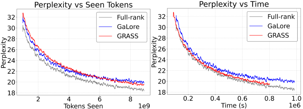
Figure 1: Pretraining 1B LLaMA on 8.8B tokens of C4 with Grass, Full-rank and GaLore. (Left) Train perplexity vs seen tokens. (Right) Train perplexity vs wall-clock time. Grass outperforms GaLore and shows $<0.01$ perplexity gap with Full-rank loss curve in wall-clock time.

Results.

As shown in Table 2, Grass matches GaLore and approaches Full-rank’s performance within a perplexity gap of less than $1$ even when $r/d_{model}=8$. In Figure 1, for the 1B model we see that this gap disappears when we look at perplexity vs. training time (as opposed to tokens seen) on a single A100 GPU, where due to increased pretraining throughput Grass closely follows the Full-rank loss curve with $<0.1$ perplexity gap.

4.2 Finetuning Performance

Model	COLA	MNLI	MRPC	QNLI	QQP	RTE	SST2	STSB	WNLI	Average
Full-rank	59.62	87.36	91.51	92.60	90.43	79.03	94.49	90.38	56.34	82.42
LoRA	58.36	86.80	90.09	92.49	89.43	75.09	94.49	90.22	56.34	81.48
GaLore	57.64	87.40	88.97	92.86	88.94	76.17	94.49	89.76	56.34	81.40
Flora	59.65	86.65	89.82	92.09	88.61	76.34	94.27	90.06	56.34	81.53
Grass (Top-$r$)	59.16	86.92	89.60	92.42	88.65	76.37	94.15	90.13	56.34	81.53
Grass (Multi-Norm2-NR)	58.87	86.08	89.94	91.69	83.36	76.17	94.73	90.00	56.34	81.35
Grass (Multi-Norm-R)	57.81	86.25	87.58	91.80	88.06	68.59	94.27	89.73	56.34	80.05
Grass (Uni-NR)	49.66	85.70	78.01	90.94	87.56	57.76	93.35	84.86	56.34	76.02

Table 3: Evaluating Full-rank and different memory-efficient optimization methods on the GLUE benchmark using RoBERTa-Base. Grass is competitive with LoRA and Flora but with a lower memory footprint. Values in blue represent the top three results in each column.

Experimental setup.

We evaluate Grass, LoRA, Full-rank, GaLore, and Flora on the GLUE NLU benchmark (Wang et al., 2018a) by finetuning a pretrained RoBERTa-Base model (Liu et al., 2019) with a sequence length of 128 in float32 (results on the dev set). For all the optimization methods, we restrict them to only optimize the linear layers in the attention and MLP layers for three epochs with individually tuned learning rates. We set rank $r=8$ for all the low-rank methods. For the MeSO methods, we set the update frequency $K=100$ and tune the scale factor $\alpha$ for each method. (See more details in Appendix I.)

Results.

In Table 3, Grass Top-$r$ performs competitively with LoRA, Flora, and GaLore even though Grass exhibits a reduced memory footprint and improved training throughput compared to these methods as we show in Section 4.

Model		MMLU Acc (%)
LLaMA-7b	Trainable Params	Alpaca	FLAN v2
Full	6898.3M	38.12	35.85
LoRA	159.90M	38.21	34.98
GaLore	6476.0M	37.93	34.72
Flora	6476.0M	37.86	35.16
Grass (Top-$r$)	6476.0M	38.37	36.88

Table 4: Average 5-shot MMLU accuracy for LLaMA-7B models finetuned with various methods across Alpaca and FLAN v2. Grass, Flora, GaLore, and LoRA were applied to attention and MLP layers using rank 64. Grass not only competes effectively with full training but also offers advantages in terms of lower memory usage and higher throughput compared to all baseline methods.

4.3 Instruction-finetuning Performance

Experimental setup.

We compare Grass against Full finetuning, GaLore, Flora, and LoRA on instruction finetuning using a LLaMA-7B model (Touvron et al., 2023) pretrained on 1T tokens. We finetune on Alpaca (Taori et al., 2023) (52k samples) and a 100k sample subset of FLAN v2 (Wei et al., 2021) from Tulu (Wang et al., 2023) (due to FLAN v2’s scale), using BF16 precision, batch size 64, and a source and target sequence length of 512. All methods, except for Full finetuning which updates all parameters, are restricted to only update the linear layers in the attention and MLP layers with rank $r=64$ . We finetune for 1000 steps on Alpaca (1.26 epochs) and 1500 steps on Flan v2 (1.08 epochs). Additional hyperparameters are in Appendix I. Following prior work (Touvron et al., 2023; Dettmers et al., 2023), we assess the instruction-tuned models’ average 5-shot test performance on the MMLU benchmark (Hendrycks et al., 2020) (57 tasks).

Results.

As shown in Table 4, Grass performs competitively with full-parameter finetuning, Flora, GaLore, and LoRA during instruction finetuning on both Alpaca and Flan v2. Furthermore, Section 4 demonstrates that, at $r=64$, Grass not only matches LoRA’s performance but also boasts a lower memory footprint and an 18% throughput increase. Because Grass can perform higher rank training with multiple projection matrix updates, it is expected to further outperform the rank-constrained LoRA in more challenging tasks with larger datasets.

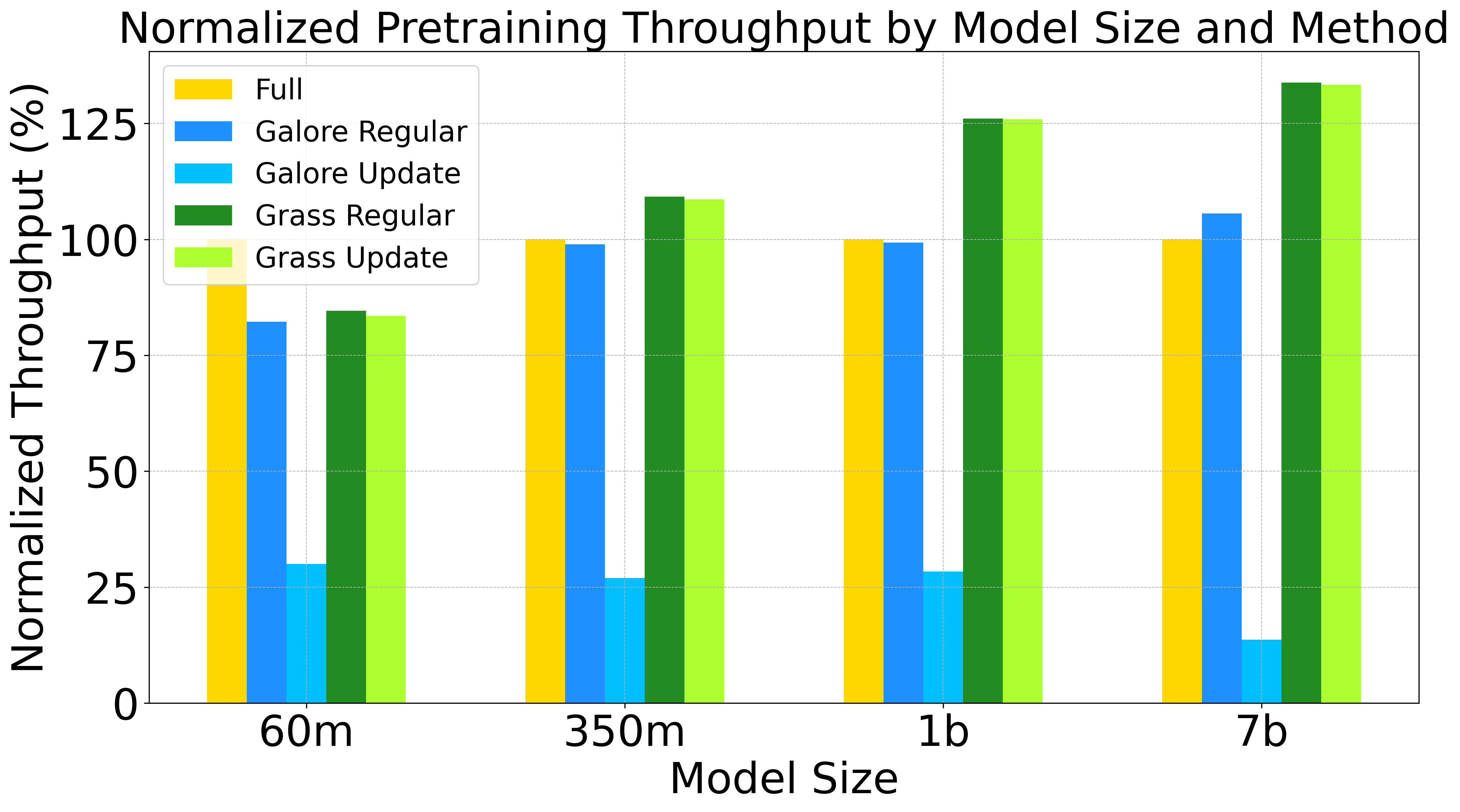
Figure 2: Normalized pretraining throughput at $r=64$ for Grass, Full-rank, and GaLore relative to Full-rank. Grass throughput exceeds Full and GaLore throughput by $>25\%$.

4.4 Efficiency analysis

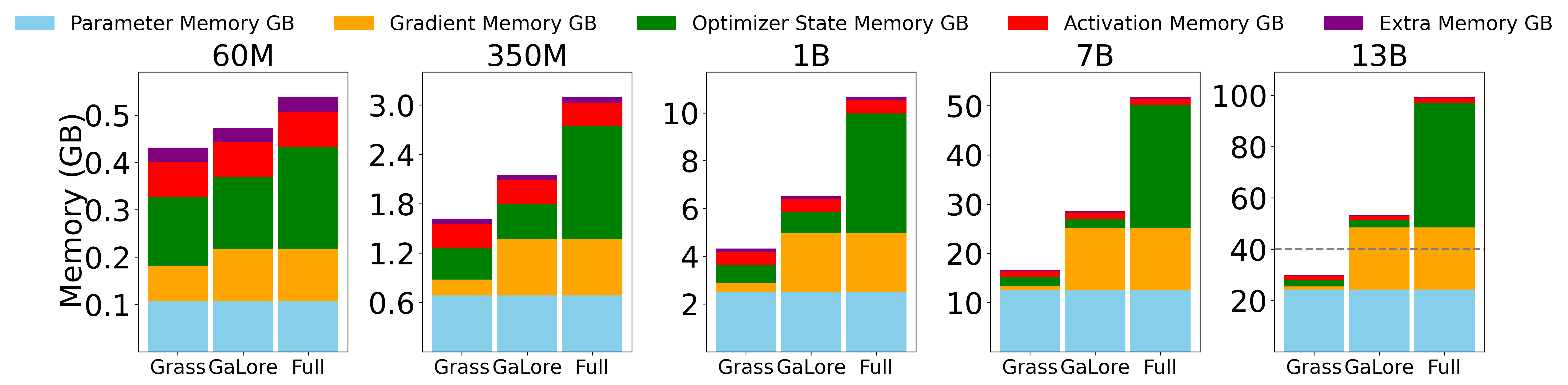
Figure 3: Pretraining memory footprint for Grass, GaLore, and Full across model sizes for a regular (non projection update step) and $r=128$. Grass has a lower memory footprint across all model sizes and the reduction is greater at larger model sizes.

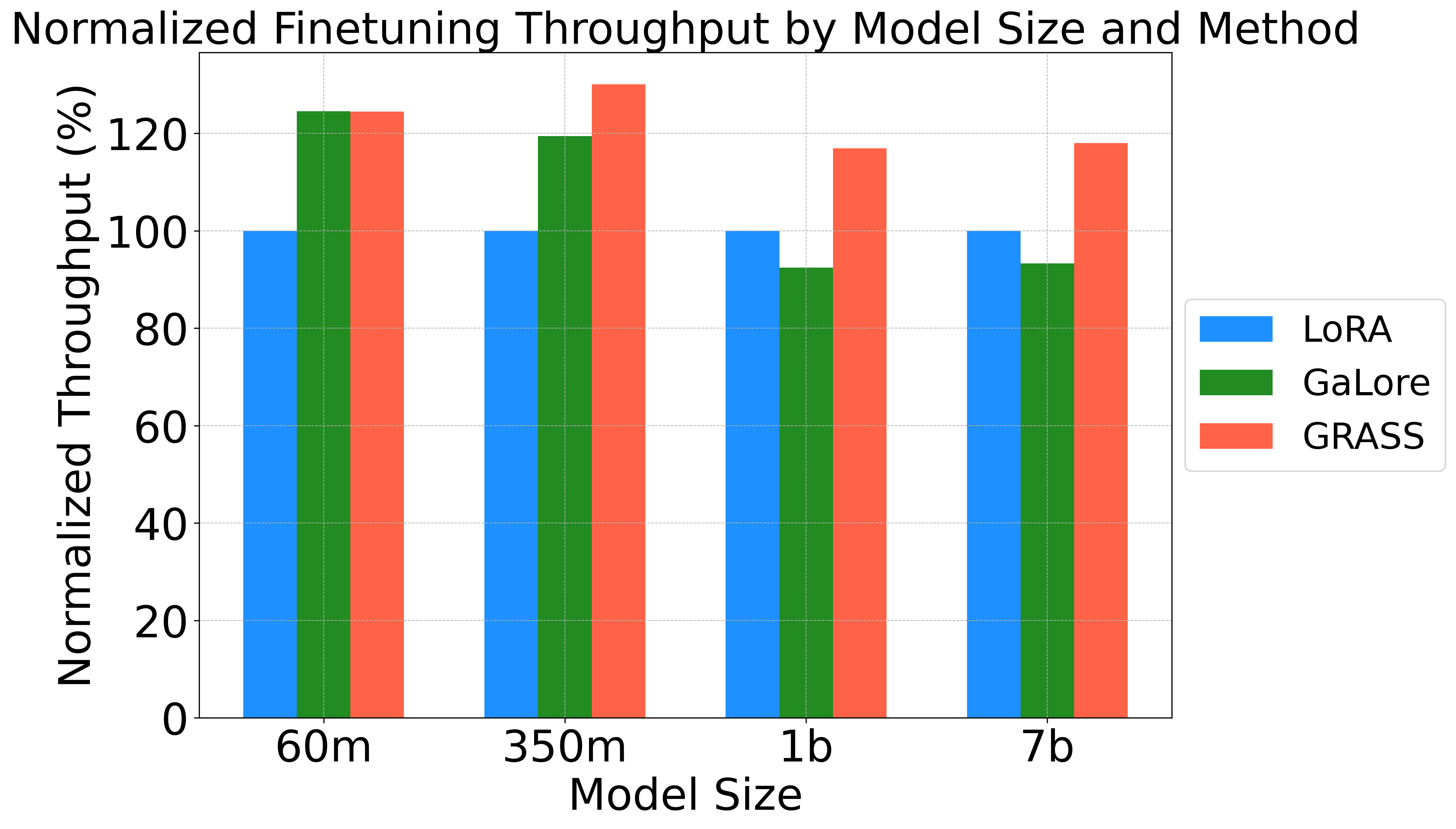
Figure 4: Normalized LLaMA finetuning throughput of Grass, GaLore, and LoRA relative to LoRA. We use rank $r=64$. Grass is $>18\%$ faster than LoRA.

Pretraining Throughput.

Figure 2 compares the BF16 pretraining throughput (tokens/s) of Grass and GaLore relative to Full-rank, across model sizes, for both regular and projection update steps. We use rank $r=64$ on attention and feedforward layers, sequence length 256, and total batch size 1024 on a single 80GB A100 GPU. See Appendix I for detailed settings. We did not employ activation checkpointing, memory offloading, or optimizer state partitioning in our experiments.

While Grass exhibits lower throughput than Full-rank at 60M parameters (due to customized matrix multiplication overhead), Grass significantly outperforms both at 1B and 7B parameters, achieving 26% and 33.8% higher throughput than Full-rank, and 27% and 26.7% higher than GaLore (for the regular step). Grass’s projection update overhead is minimal, unlike GaLore’s costly SVD computations. The throughput advantage for Grass is expected to grow with larger batch sizes, benefiting further from its lower memory footprint compared to other methods. Appendix Figure 11 provides further throughput comparisons across different ranks, showing that Grass achieves its highest relative throughput gains at rank ($r=64$), with diminishing returns as rank increases or model size decreases.

Finetuning Throughput.

Figure 4 compares the BF16 finetuning throughput of Grass, GaLore, and LoRA across various LLaMA model sizes, focusing on the regular step. Unlike the pretraining throughput benchmark, we finetune only the attention and MLP layers using $r=64$. We maintain a uniform local batch size, sequence length 256, and total batch size of 1024 across all methods (detailed hyperparameters are provided in Appendix I). For the 7B parameter model, Grass achieves throughput improvements of 26% and 18% over GaLore and LoRA, respectively. Appendix Figure 12 provides further throughput comparisons across ranks 8, 16, 32, and 64, demonstrating that Grass consistently maintains its throughput advantage across these ranks.

Pretraining Memory.

Figure 3 benchmarks the BF16 memory footprint of pretraining Grass against Full-rank and GaLore across various model sizes (token batch size 256, rank (r=128)), focusing on the regular training step. Grass consistently exhibits a lower memory footprint than both Full-rank and GaLore, with the memory reduction increasing with model size. This advantage stems from Grass’s reduced gradient and optimizer memory (due to its sparse projection matrices). At 13B parameters, Grass uses 70% less memory than Full-rank and 45% less than GaLore.

Beyond the memory advantage in the regular update iteration, Grass is also more memory efficient in the projection update iteration compared to its counterpart GaLore: GaLore requires converting the full gradient to float32 for SVD computation when computing the projection matrix, making it unable to pretrain the 13B LlaMA model in BF16 at rank (r = 128) on an 80GB GPU. In contrast, Grass is capable of pretraining the 13B model on ranks up to $r=768$ on a 40GB GPU and up to $r=1024$ on a 48GB GPU.

Finetuning Memory.

Appendix Figure 9 and Figure 10 compare the memory footprint of Grass and LoRA during LLaMA finetuning. Grass demonstrates a memory advantage of roughly 1GB over LoRA when finetuning the 7B parameter model in BF16 at rank (r=64). However, as the batch size increases, activations dominate the memory footprint, and the memory usage of Grass and LoRA becomes comparable.

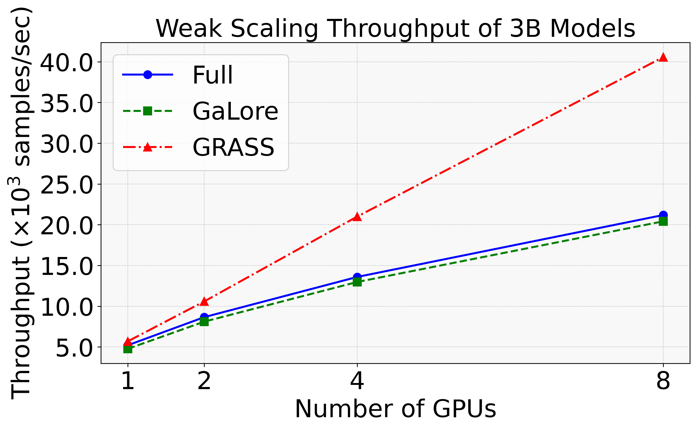
Figure 5: Communication Efficiency: Weak Scaling Throughput Comparison for 3B LLaMA pretraining using Grass, Full-rank, and GaLore. Grass shows $2\times$ higher throughput over Full and GaLore at 8 GPUs.

Communication.

Figure 5 benchmarks the (weak scaling (Gustafson, 1988)) throughput (tokens/sec) of training a 3B parameter LLaMA model on a multi-GPU L40 compute node with a peak all-reduce bandwidth of 8.64 GB/s as we scale the number of participating GPUs. We use a token batch size of 4096 per worker (local batch size 16, sequence length 256). Grass, by communicating only the projected gradients, achieves significantly higher throughput (2$\times$ on 8 GPUs) compared to both Full-rank and GaLore.

4.5 Ablations

Effect of Rank.

Figure 6 presents ablations on the impact of the subspace rank $r$ for Grass during pretraining of a 350M parameter LLaMA model on the C4 subset of Dolma. Increasing the rank generally leads to better training losses for the same number of updates, but with diminishing returns. Additionally, since Grass enables full-parameter training, we observe that training at rank $r=128$ for 80k steps is more effective than training at rank $r=512$ for 40k steps. Grass can therefore be used to trade-off memory and computational cost where in a memory-constrained setting one could select a lower rank and train longer.

Figure 6: Grass rank ablations for 350M LLaMA training. We report perplexity on Dolma C4 across various ranks and training steps. Loss is averaged over a window of 50 steps.

Effect of Update Frequency.

Figure 7 analyzes the impact of update frequency on the convergence of Grass during pretraining of a 60M-parameter LLaMA model on the Realnews subset of C4 (Raffel et al., 2020). Both overly frequent and infrequent updates to the projection matrix hinder convergence. Optimal convergence is achieved within an update frequency range of 200 to 500 iterations.

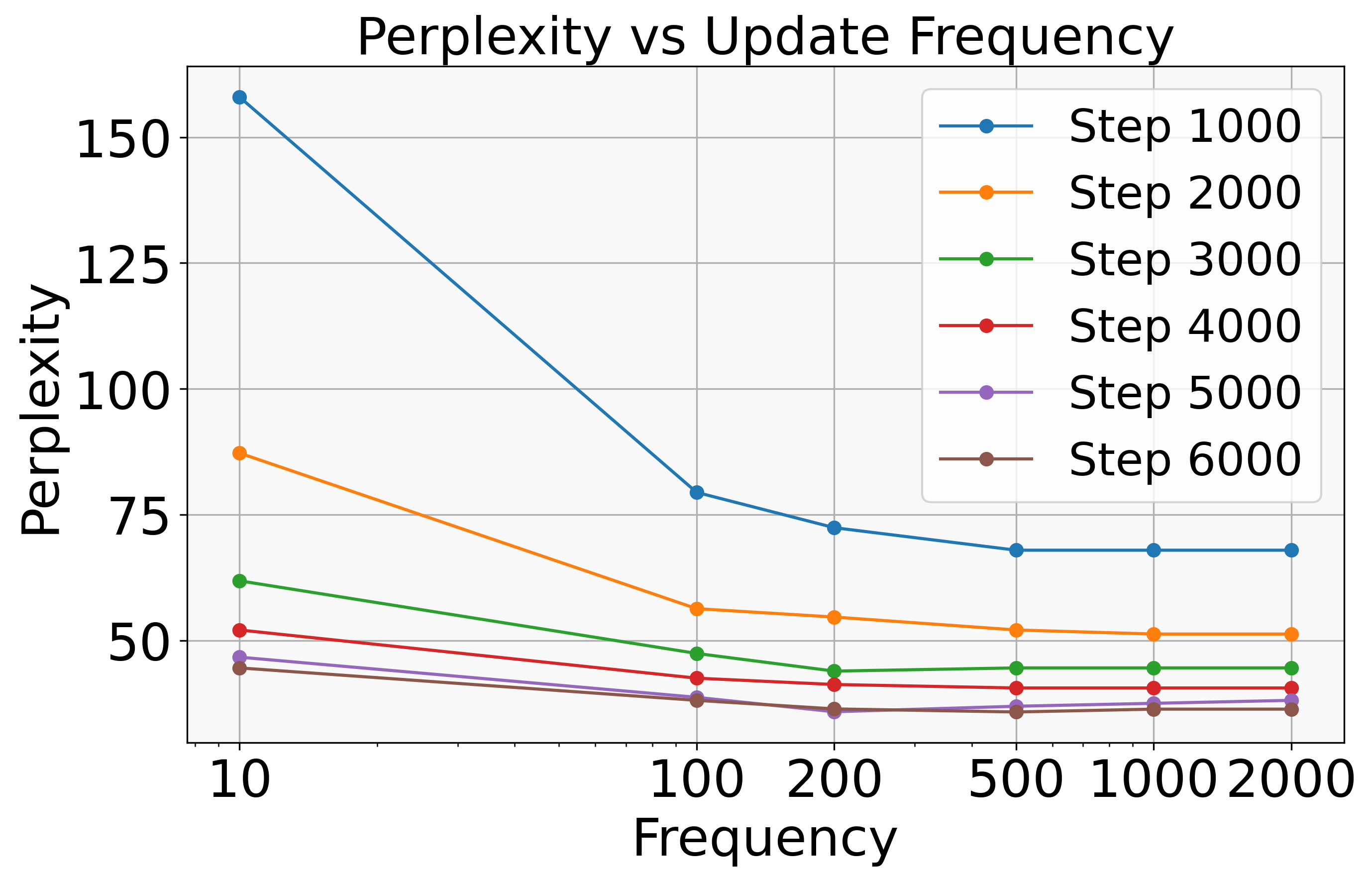
Figure 7: Grass Update Frequency vs. Training Perplexity for 60M LLaMA pretraining on Realnews subset of C4. A frequency of 200 is near optimal.

compute_P Methods.

Sampling Method	Eval perp
Frozen Top-$r$	34.78
Uniform-R	32.46
Uniform-NR	31.06
Multinomial-Norm-R	31.32
Multinomial-Norm-NR	30.93
Multinomial-Norm2-R	31.85
Multinomial-Norm2-NR	30.91
Top-$r$	30.88
GaLore	30.67
Full-rank	30.27

Table 5: Comparison of Grass Sampling Methods on Evaluation Perplexity during 60M LLaMA Pretraining on the RealNews Subset of C4. Best sampling strategy is bolded.

Table 5 evaluates our proposed methods to compute the sparse projection $P$ matrix (in Section 3.2) for Grass during pretraining of a 60M LLaMA model on 500M tokens from the RealNews subset of C4. We additionally consider the Frozen Top-$r$ method as a baseline by computing top indices once only at iteration 0. We notice that stochastic strategies employing non-replacement biased (NR) sampling generally surpass their with replacement unbiased (R) counterparts. Within the unbiased strategies (R), the variance reduction approach (Multinomial-Norm-R) outperforms the subspace preservation method (Multinomial-Norm²-R), while their biased (NR) counterparts exhibit comparable performance. Both Multinomial-Norm²-NR and Top-$r$ are competitive with GaLore, while Uniform sampling underperforms. Similar trends in performance across sampling methods are observed during finetuning (Table 3). We find that uniform sampling is more effective for pretraining than finetuning, likely because the norm distribution is more uniform at the onset of pretraining.

5 Conclusion And Future Work

In this work, we introduce Grass, a novel memory-efficient subspace optimization method for LLM pretraining and fine-tuning by leveraging sparse gradient projections. Grass significantly reduces the memory footprint of optimizer states and gradients and eliminates the need to materialize the full gradients during the projection step, leading to substantial computational efficiency gains. Our experimental results demonstrate that Grass achieves comparable performance to full-rank training and existing projection-based methods while offering a substantial memory reduction and throughput increase across various model sizes and tasks. Future work will explore extending Grass to utilize diverse structured sparsity patterns and investigating strategies for dynamically adjusting the projection rank based on hardware and model size.

6 Limitations

While Grass offers compelling advantages in memory efficiency and training throughput, there are several aspects that warrant further investigation and potential improvements.

Implementation Complexity.

Unlike drop-in optimizer replacements, Grass requires integrating custom linear layers into the Transformer architecture, as the sparse projection operations occur during the backward pass. While this involves minimal code modifications, it introduces a slight complexity barrier for adoption compared to simply switching optimizers. Nonetheless, the significant gains in performance and memory efficiency outweigh this minor overhead.

Scalability to Larger Models.

Our empirical evaluation primarily focused on model scales up to 13B parameters. The effectiveness of Grass for significantly larger LLMs, exceeding hundreds of billions of parameters, requires further examination. Similarly, as batch sizes increase, the memory savings from sparse projection might become less prominent compared to the activation memory footprint. Exploring strategies to mitigate this potential issue, such as combining Grass with activation checkpointing techniques, would be beneficial.

Hyperparameter Sensitivity.

Grass’s performance depends on hyperparameters like rank $(r)$ and update frequency $(K)$. While our experiments provide insights into suitable ranges for these hyperparameters, a more comprehensive analysis of their impact on training dynamics, particularly as model scales increase, is crucial for maximizing performance and generalizability. Developing methods to automatically and adaptively tune these hyperparameters could further enhance Grass’s applicability.

7 Ethical Considerations

We acknowledge the potential ethical implications associated with large language models. These include:

Misuse Potential.

LLMs, being powerful text generation tools, can be misused to create harmful or misleading content, including disinformation, hate speech, and spam. While our work focuses on improving training efficiency, we strongly advocate for responsible use of LLMs and encourage further research on safeguards against malicious applications.

Bias Amplification.

LLMs are trained on massive text corpora, which can inherently contain biases and stereotypes. These biases can be amplified during training, leading to potentially discriminatory or unfair outputs. While Grass is unlikely to exacerbate this bias, we recognize the importance of addressing this issue through careful data curation, bias mitigation techniques, and ongoing monitoring of LLM behavior.

Environmental Impact.

Training large LLMs requires significant computational resources, which can have a substantial environmental footprint. Our work aims to reduce the computational cost and energy consumption of LLM training, contributing to more sustainable and environmentally responsible practices in NLP research.

Data and Licensing Considerations.

We have carefully considered the ethical implications of the datasets used in this work which are publicly released and have followed accepted privacy practices at creation time.

• MMLU and GLUE are released under the permissive MIT license, allowing for broad research use.

• Alpaca is also distributed under the MIT license.

• FLAN uses the Apache license, which permits both academic and commercial applications.

• Dolma utilizes the ODC Attribution License, promoting open data sharing and reuse.

We strictly adhere to the license terms and intended use of these datasets, ensuring responsible handling of data and compliance with ethical guidelines. We acknowledge the ongoing need for critical assessment and transparency regarding data sources, potential biases, and licensing implications in LLM research.

Appendix A Optimizer Functions

In Equation (1) and Algorithm 1, we use functions opt.init and opt.update to abstractly represent any stateful optimizer’s initialization and update function. Here we provide concrete implementations of these functions for Adam (Kingma and Ba, 2014) in Algorithm 3 and 4. We assume the parameter matrix $Z$ and its gradient $\nabla_{Z}L$ is of generic shape $\mathbb{R}^{c\times d}$.

Algorithm 3 Initialization of the Adam optimizer, adam.init

1:$Z\in\mathbb{R}^{c\times d}$ (technically, Adam only requires knowing the shape of the parameter)

2:$S\in\mathbb{R}^{2\times c\times d}$  

3:$M\leftarrow\mathbf{0}_{c\times d}$ $\triangleright$ First gradient moment statistics

4:$V\leftarrow\mathbf{0}_{c\times d}$ $\triangleright$ Second gradient moment statistics

5:$S\leftarrow(M,V)$

Algorithm 4 Update of the Adam optimizer, adam.update. $\beta_{1},\beta_{2}\in[0,1)$ are the exponential decay rates for the first and second gradient moment estimates. $t$ is the current iteration. $\eta>0$ is the current iteration’s learning rate. $\epsilon$ is a small constant used for numerical stability in division.

1:$S\in\mathbb{R}^{2\times c\times d}$ the most recent optimizer state $\nabla L(Z)\in\mathbb{R}^{c\times d}$ the current gradient of $Z$

2:$S_{\textrm{new}}\in\mathbb{R}^{2\times c\times d}$ the updated optimizer state  $U\in\mathbb{R}^{c\times d}$ the additive update matrix  

3:$M,V\leftarrow S$ $\triangleright$ Unpack the states $M,V\in\mathbb{R}^{c\times d}$

4:$M_{\textrm{new}}\leftarrow\beta_{1}\cdot M+(1-\beta_{1})\cdot\nabla L(Z)$

5:$V_{\textrm{new}}\leftarrow\beta_{2}\cdot V+(1-\beta_{2})\cdot\nabla L(Z)^{\circ 2}$

6:$S_{\textrm{new}}\leftarrow(M_{\textrm{new}},V_{\textrm{new}})$

7:$M_{\star}\leftarrow M_{\textrm{new}}/(1-\beta_{1}^{t})$

8:$V_{\star}\leftarrow V_{\textrm{new}}/(1-\beta_{2}^{t})$

9:$U\leftarrow-\eta\cdot M_{\star}\oslash(V_{\star}^{\circ\frac{1}{2}}+\epsilon\cdot\mathbf{1}_{c\times d})$

Appendix B Derivation of the Unified Algorithm of Memory-efficient Subspace Optimizers

As we have described in Section 2, MeSO optimizers solve the subspace optimization problem under the projection matrix $P\in\mathbb{R}^{m\times r}$:

$$\min_{A\in\mathbb{R}^{r\times n}}L(W_{0}+PA)$$ (2)

by applying an off-the-shelf optimizer opt. Since we want to start at the initial weight matrix $W_{0}$, $A$ is initialized to be the zero matrix:

$$A^{(0)} \leftarrow 0_{r\times n}$$ (3)

$$S^{(0)} \leftarrow\texttt{opt.update}(A^{(0)})$$ (4)

and updated through

$$S^{(t+1)},\Delta^{(t+1)} \leftarrow\texttt{opt.update}(S^{(t)},\frac{d}{dA}L(W_{0}+PA^{(t)}))$$ (5)

$$A^{(t+1)} \leftarrow A^{(t)}+\Delta^{(t+1)}$$ (6)

By chain rule, we have $\frac{d}{dA}L(W_{0}+PA^{(t)})=P^{\top}\nabla L(W_{0}+PA^{(t)})$.

When MeSO updates the projection matrix to be $P_{\textrm{new}}$, we can treat the new subspace optimization as having its $W_{0}^{\textrm{new}}=W_{0}^{\textrm{old}}+P_{\textrm{old}}A^{(t)}$ and re-initializing $A^{(t)}$ at $0_{r\times n}$ in addition to an optimizer state update using . The pseudocode of this algorithm where we maintain the value of the $A$ matrix is given in Algorithm 5.

Algorithm 5 Memory-efficient subspace optimization (MeSO) with an instantiated $A$ matrix

1:Initial weights $W_{0}\in\mathbb{R}^{m\times n}$ with $m\leq n$; update frequency $K$; total iterations $T$; subspace rank $r$ with $r\ll m$, an off-the-shelf optimizer opt; function to update the optimizer state, scale factor $\alpha$.

2:Optimized weights $W^{(T)}$  

3:$t\leftarrow 0$

4:$A^{(0)}\leftarrow 0_{r\times n}$

5:$S^{(0)}\leftarrow\texttt{opt.init}(A^{(0)})$ $\triangleright$ Adam state $\in\mathbb{R}^{r\times n}$

6:while $t\leq T$ do

7:     if $t\equiv 0\pmod{K}$ then

8:         $W_{0}\leftarrow W_{0}+PA^{(t)}$ $\triangleright$ record progress

9:         $A^{(t)}\leftarrow 0_{r\times n}$ $\triangleright$ reinitialize $A$

10:         // Compute new projection matrix

11:         $P\leftarrow$ $\texttt{compute}_{P}$ $(\nabla L(W_{0}))$ $\triangleright$ $P\in\mathbb{R}^{m\times r}$

12:         // [Optional] Update optimizer state

13:         $S^{(t)}\leftarrow\texttt{update\_state}(S^{(t)})$

14:     end if

15:     $G_{C}\leftarrow P^{\top}\nabla L(W_{0}+PA^{(t)})$ $\triangleright$ $G_{C}\in\mathbb{R}^{r\times n}$

16:     $S^{(t+1)},\Delta^{(t+1)}\leftarrow\texttt{opt.update}(S^{(t)},G_{C})$

17:     $A^{(t+1)}\leftarrow A^{(t)}+\alpha\Delta^{(t+1)}$ $\triangleright$ Apply Update

18:     $t\leftarrow t+1$

19:end while

By defining $W^{(t)}\coloneqq W_{0}+PA^{(t)}$, we can easily see that Algorithm 5 is equivalent to Algorithm 1 presented in the main paper.

Appendix C Additional Related Work

Memory-Efficient Optimization.

Several works aim to reduce the memory footprint of adaptive optimizer states. Techniques include factorizing second-order moment statistics (Shazeer and Stern, 2018), quantizing optimizer states (Dettmers et al., 2021; Anil et al., 2019; Dettmers et al., 2023; Li et al., 2023), and fusing backward operations with optimizer updates to minimize gradient storage (Lv et al., 2023a). Grass is orthogonal to these approaches and proposes a gradient projection-based adaptive optimizer that significantly reduces memory costs by relying on projected gradient statistics.

Gradient Compression.

In distributed and federated training, several gradient compression methods have been introduced to reduce the volume of transmitted gradient data. Common approaches include:

1. Quantization: Quantization aims to reduce the bit precision of gradient elements. Examples include 1-bit SGD (Seide et al., 2014), SignSGD (Bernstein et al., 2018), 1-bit Adam (Tang et al., 2021), TernGrad (Wen et al., 2017), and QSGD (Alistarh et al., 2017).

2. Sparsification: This involves transmitting only a small subset of significant gradient elements. Random-$k$ and Top-$k$ element select $k$ random or largest-magnitude elements, respectively to transmit. Top-$k$ generally exhibits better convergence (Stich et al., 2018), and requires communicating both values and indices (Lin et al., 2018; Renggli et al., 2019).

3. Low-Rank Decomposition: This involves factorizing a gradient matrix $M\in\mathbb{R}^{n\times m}$ as $M\approx PQ^{\top}$ for transmission, where $P\in\mathbb{R}^{n\times r}$ and $Q\in\mathbb{R}^{m\times r}$ with $r\ll\min(n,m)$. ATOMO (Wang et al., 2018b) employs SVD for decomposition, while Power-SGD (Vogels et al., 2019) utilizes power iteration for more efficient low-rank factorization.

Unlike existing methods, Grass introduces a novel approach by employing sparse projection of gradients to enhance memory efficiency in both local and distributed training contexts.

Appendix D Ensuring Unbiased Gradient Reconstruction

In this section, we formally state the theorem that gives the form of the sampling distribution for $\sigma_{j}$ and $\rho_{jj}$ that ensures the reconstructed gradient $PP^{\top}G_{W}$ is unbiased which we describe in Section 3.2.

Theorem D.1.

Let $B\in\{0,1\}^{r\times m}$ be the sparse binary matrix with the unique non-zero index of $j$-th row being $\sigma_{j}\in[m]$. Let $\sigma_{j}\stackrel{{\scriptstyle\textit{i.i.d.}}}{{\sim}}\textrm{Multinomial}(1,q)$) ($q\in\mathbb{R}^{m}$ with the probability of sampling integer $k\in[m]$ being $q_{k}$). If we correspondingly let the diagonal value of the diagonal matrix $\rho$ to be $\rho_{jj}\coloneqq\frac{1}{\sqrt{rq_{\sigma_{j}}}}$, then for the random projection matrix $P=(\rho B)^{\top}$, we have $\mathbb{E}[PP^{\top}G]=G$ for any (gradient) matrix $G\in\mathbb{R}^{m\times n}$.

Proof.

Here we first write down the form of the random matrix product $PP^{\top}$. Let $e_{j}\in\mathbb{R}^{m}$ be the unit column vector with $j$-th coordinate being 1 and all other coordinates being zero. Then by definition, the $j$-th row vector of $B$ is $e_{\sigma_{j}}^{\top}$.

$$PP^{\top}$$ (7)

$$= B^{\top}\rho^{\top}\rho B$$ (8)

$$= \begin{bmatrix}{\hbox to0.0pt{\leavevmode\hbox{\set@color$e_{\sigma_{1}}$}\hss}\hskip 4.72809pt\makebox[0.0pt][c]{\rule[5.30554pt]{0.5pt}{5.0pt}}\makebox[0.0pt][c]{\rule[-8.23666pt]{0.5pt}{5.0pt}}\hskip 4.72809pt}&\ldots&{\hbox to0.0pt{\leavevmode\hbox{\set@color$e_{\sigma_{r}}$}\hss}\hskip 4.69438pt\makebox[0.0pt][c]{\rule[5.30554pt]{0.5pt}{5.0pt}}\makebox[0.0pt][c]{\rule[-7.89444pt]{0.5pt}{5.0pt}}\hskip 4.69438pt}\end{bmatrix}_{m\times r}$$

$$\qquad\times\mathrm{diag}(\frac{1}{r\cdot q_{\sigma_{1}}},\ldots,\frac{1}{r\cdot q_{\sigma_{r}}})$$

$$\qquad\qquad\times\begin{bmatrix}-e_{\sigma_{1}}^{\top}-\\ \vdots\\ -e_{\sigma_{r}}^{\top}-\end{bmatrix}_{r\times m}$$ (9)

$$= \frac{1}{r}\sum_{i=1}^{r}\frac{1}{q_{\sigma_{i}}}e_{\sigma_{i}}e_{\sigma_{i}}^{\top}$$ (10)

In Equation 10, we have decomposed the matrix $PP^{\top}$ into the average of $r$ random rank-1 matrices each of which depends on on the randomness of a unique $\sigma_{i}$. By linearity of expectation and the i.i.d. property of $\{\sigma_{i}\}_{i=1}^{r}$, we have

$$\mathbb{E}[PP^{\top}]= \frac{1}{r}\sum_{i=1}^{r}\mathbb{E}[\frac{1}{q_{\sigma_{i}}}e_{\sigma_{i}}e_{\sigma_{i}}^{\top}]$$ (11)

$$= \mathbb{E}[\frac{1}{q_{\sigma_{{\color[rgb]{0,0,1}1}}}}e_{\sigma_{{\color[rgb]{0,0,1}1}}}e_{\sigma_{{\color[rgb]{0,0,1}1}}}^{\top}]$$ (12)

Since $\sigma_{1}$ have a probability of $q_{k}$ to take the value of integer $k\in[m]$, we have

$$\mathbb{E}[\frac{1}{q_{\sigma_{{\color[rgb]{0,0,1}1}}}}e_{\sigma_{{\color[rgb]{0,0,1}1}}}e_{\sigma_{{\color[rgb]{0,0,1}1}}}^{\top}]$$ (13)

$$= \sum_{k=1}^{m}q_{k}\cdot\frac{1}{q_{k}}e_{k}e_{k}^{\top}$$ (14)

$$= I_{m\times m}$$ (15)

Thus we have proved that $\mathbb{E}[PP^{\top}]=I_{m\times m}$. By linearity of expectation, for any matrix $G\in\mathbb{R}^{m\times n}$, we thus have $\mathbb{E}[PP^{\top}G]=G$ and the proof is complete. ∎

Appendix E Proof of Theorem 3.1

Here we restate the complete version of Theorem 3.1 and then present its proof.

Theorem (Complete statement of Theorem 3.1).

Let $B\in\{0,1\}^{r\times m}$ be the sparse binary matrix with the unique non-zero index of $j$-th row being $\sigma_{j}\in[m]$. Let $\sigma_{j}\stackrel{{\scriptstyle\textit{i.i.d.}}}{{\sim}}\textrm{Multinomial}(1,q)$ ($q\in\mathbb{R}^{m}$ with the probability of sampling integer $k\in[m]$ being $q_{k}$). Given $\sigma_{j}$, we correspondingly set the diagonal value of the diagonal matrix $\rho$ to be $\rho_{jj}\coloneqq\frac{1}{\sqrt{rq_{\sigma_{j}}}}$ and define $P=(\rho B)^{\top}$. This induces an unbiased gradient estimator of $G\in\mathbb{R}^{m\times n}$: $PP^{T}G$. Among all these gradient estimators induced by different parameter value $q$ of the multinomial distribution, the one that is proportional to the row norms of $G$ with $q_{k}=\frac{\|G_{k}\|_{2}}{\sum_{i=1}^{m}\|G_{i}\|_{2}}$ minimizes the total variance of the gradient estimate $PP^{\top}G$.

Proof.

We first write down the total variance of the estimator $PP^{\top}G$:

$$\mathbb{E}\;\mathrm{tr}[(PP^{\top}G)^{\top}(PP^{\top}G)]$$

$$\qquad-\mathrm{tr}[\mathbb{E}[(PP^{\top}G)]\mathbb{E}[(PP^{\top}G)]^{\top}]$$ (16)

$$= \mathrm{tr}[G^{\top}\mathbb{E}[PP^{\top}PP^{\top}]G]-\mathrm{tr}[GG^{\top}]$$ (17)

Since only the first term in Equation 17 is a function of $P$ and thus depends on the value of $q$, we first focus on analytically deriving the form of $\mathbb{E}[PP^{\top}PP^{\top}]$.

By the expression in Equation 10, we have:

$$PP^{\top}PP^{\top}$$ (18)

$$= \;\frac{1}{r^{2}}\sum_{i=1}^{r}\sum_{j=1}^{r}\frac{1}{q_{\sigma_{i}}}\frac{1}{q_{\sigma_{j}}}e_{\sigma_{i}}e_{\sigma_{i}}^{\top}e_{\sigma_{j}}e_{\sigma_{j}}^{\top}$$ (19)

$$= \;\frac{1}{r^{2}}\sum_{i=1}^{r}\frac{1}{q_{\sigma_{i}}^{2}}e_{\sigma_{i}}e_{\sigma_{i}}^{\top}e_{\sigma_{i}}e_{\sigma_{i}}^{\top}$$

$$\quad+\frac{1}{r^{2}}\sum_{i=1,j=1,i\neq j}^{r}[\frac{1}{q_{\sigma_{i}}}e_{\sigma_{i}}e_{\sigma_{i}}^{\top}][\frac{1}{q_{\sigma_{j}}}e_{\sigma_{j}}e_{\sigma_{j}}^{\top}]$$ (20)

$$= \;\frac{1}{r^{2}}\sum_{i=1}^{r}\frac{1}{q_{\sigma_{i}}^{2}}e_{\sigma_{i}}e_{\sigma_{i}}^{\top}$$

$$\quad+\frac{1}{r^{2}}\sum_{i=1,j=1,i\neq j}^{r}[\frac{1}{q_{\sigma_{i}}}e_{\sigma_{i}}e_{\sigma_{i}}^{\top}][\frac{1}{q_{\sigma_{j}}}e_{\sigma_{j}}e_{\sigma_{j}}^{\top}]$$ (21)

In the last step, we use the fact that for any $i$, $e_{\sigma_{i}}^{\top}e_{\sigma_{i}}=1$. Now we take the expectation of Equation 21. By applying linearity of expectation and the i.i.d. property of $\{\sigma_{j}\}$, we have

$$\mathbb{E}[PP^{\top}PP^{\top}]$$ (22)

$$= \frac{1}{r}\mathrm{diag}(\frac{1}{q_{1}},\ldots,\frac{1}{q_{m}})+\frac{r-1}{r}\cdot I_{m\times m}$$ (23)

As a result, we can express the first term in Equation 17 as

$$\mathrm{tr}[G^{\top}\mathbb{E}[PP^{\top}PP^{\top}]G]$$ (24)

$$= \frac{1}{r}\mathrm{tr}[G^{\top}\mathrm{diag}(\frac{1}{q_{1}},\ldots,\frac{1}{q_{m}})G]+\frac{r-1}{r}\mathrm{tr}[GG^{\top}]$$ (25)

If we represent the rows of $G$ as column vectors $\{G_{k}\}_{k=1}^{m}$, then the only term in Equation 25 that depends on $q$ can be expressed as

$$\mathrm{tr}[G^{\top}\mathrm{diag}(\frac{1}{q_{1}},\ldots,\frac{1}{q_{m}})G]$$ (26)

$$= \mathrm{tr}[\sum_{k=1}^{m}\frac{1}{q_{k}}G_{k}G_{k}^{\top}]$$ (27)

$$= \sum_{k=1}^{m}\frac{1}{q_{k}}\mathrm{tr}[G_{k}G_{k}^{\top}]$$ (28)

$$= \sum_{k=1}^{m}\frac{\|G_{k}\|_{2}^{2}}{q_{k}}$$ (29)

Based on these derivations, to minimize the total variance is therefore equivalent to minimize Equation 29. From now on, we denote $\lambda_{i}\coloneqq\|G_{i}\|_{2}$ as the 2-norm of the $i$-th row of matrix $G$.

Solving the variance-minimization problem:

As we have shown, minimizing the total variance of $PP^{\top}G$ leads to the following optimization problem:

$$\min_{p} \sum_{i=1}^{m}\frac{\lambda_{i}^{2}}{q_{i}}$$ (30)

$$\text{subject to}\quad\sum_{i=1}^{n}q_{i}= 1,\quad q_{i}\geq 0\text{ for all }i.$$

Here we first ignore the inequality constraint $q_{i}\geq 0$ and solve the relaxed problem:

$$\min_{p} \sum_{i=1}^{m}\frac{\lambda_{i}^{2}}{q_{i}}$$ (31)

subject to $$\quad\sum_{i=1}^{n}q_{i}=1$$

The Lagrangian $L$ for this relaxed constrained optimization is:

$$L(q,\mu)=\sum_{i=1}^{m}\frac{\lambda_{i}^{2}}{q_{i}}+\mu\left(\sum_{i=1}^{m}q_{i}-1\right)$$

where $\mu$ is the Lagrange multiplier for the equality constraint. The stationary condition for the Lagrangian gives us

$$\frac{\partial L}{\partial q_{i}}=-\frac{\lambda_{i}^{2}}{q_{i}^{2}}+\mu=0,\;\;\forall i\in[m]$$ (32)

$$\sum_{i=1}^{m}q_{i}=1$$ (33)

Assuming not all $\lambda_{i}$ are zero, this gives us

$$q_{i}^{*}=\frac{\lambda_{i}}{\sum_{j=1}^{m}\lambda_{j}}$$

Since this optimal solution to Equation 31 also lies in the constraint space of Equation 30, this is also the optimal solution of the optimization we care about.

Thus we have shown that the distribution parameter $q$ that minimizes the total variance of the gradient estimate is proportional to the row 2-norm of $G$.

∎

Appendix F Row Norms and Subspace Embedding Property

The following proof is from Magdon-Ismail (2010) which can be roughly stated as sampling with squared row-norms preserves subspaces up to additive error with high probability.

Theorem F.1 (Subspace Preservation).

Let $\mathbf{A}\in\mathbb{R}^{m\times d_{1}}$ with rows $\mathbf{a}_{t}$. Define a sampling matrix $\mathbf{Q}\in\mathbb{R}^{m\times m}$ using row-sampling probabilities:

$$p_{t}\geq\frac{\|\mathbf{a}_{t}\|^{2}}{\|\mathbf{A}\|_{F}^{2}}.$$

If $r\geq\frac{4p_{A}\ln\frac{2d_{1}}{\delta}}{\beta^{2}}$, then with probability at least $1-\delta$, it follows that:

$$\|\mathbf{A}^{\top}\mathbf{A}-\tilde{\mathbf{A}}^{\top}\tilde{\mathbf{A}}\|\leq\epsilon\|\mathbf{A}\|^{2}.$$

Proof.

Considering the singular value decompositions (SVDs) of $\mathbf{A}$ and $\mathbf{B}$, we have:

$$\|\mathbf{A}^{\top}\mathbf{B} -\mathbf{A}^{\top}\mathbf{Q}^{\top}\mathbf{Q}\mathbf{B}\|=\|\mathbf{V}_{A}\mathbf{S}_{A}\mathbf{U}_{A}^{\top}\mathbf{U}_{B}\mathbf{S}_{B}\mathbf{V}_{B}^{\top}$$

$$-\mathbf{V}_{A}\mathbf{S}_{A}\mathbf{U}_{A}^{\top}\mathbf{Q}^{\top}\mathbf{Q}\mathbf{U}_{B}\mathbf{S}_{B}\mathbf{V}_{B}^{\top}\|.$$

We may now directly apply Lemma F.2, with respect to the appropriate sampling probabilities. One can verify that the sampling probabilities are proportional to the sum of the rescaled squared norms of the rows of $\mathbf{A}$ and $\mathbf{B}$. ∎

Lemma F.2 (Sampling in Orthogonal Spaces).

Let $\mathbf{W}\in\mathbb{R}^{m\times d_{1}}$ and $\mathbf{V}\in\mathbb{R}^{m\times d_{2}}$ be orthogonal matrices, and let $\mathbf{S}_{1}$ and $\mathbf{S}_{2}$ be positive diagonal matrices in $\mathbb{R}^{d_{1}\times d_{1}}$ and $\mathbb{R}^{d_{2}\times d_{2}}$, respectively. Consider row sampling probabilities:

$$p_{t}\geq\frac{1}{\|\mathbf{S}_{1}\|_{F}^{2}}\mathbf{W}^{\top}\mathbf{S}_{1}^{2}\mathbf{W}_{t}+\frac{1}{\|\mathbf{S}_{2}\|_{F}^{2}}\mathbf{V}^{\top}\mathbf{S}_{2}^{2}\mathbf{V}_{t}.$$

If $r\geq\left(8(p_{1}+p_{2})/\beta^{2}\right)\ln\frac{2(d_{1}+d_{2})}{\delta}$, then with probability at least $1-\delta$, it holds that:

$$\|\mathbf{S}_{1}\mathbf{W}^{\top}\mathbf{V}\mathbf{S}_{2}-\mathbf{S_{1}}\mathbf{W}^{\top}\mathbf{Q}^{\top}\mathbf{Q}\mathbf{V}\mathbf{S}_{2}\|\leq\epsilon\|\mathbf{S}_{1}\|\|\mathbf{S}_{2}\|.$$

Appendix G Detailed Breakdown of Compute, Memory, and Communication Volume

In this section we provide detailed breakdown of the compute, memory, and communication volume for different optimization methods. We focus our discussion to a single weight matrix $W\in\mathbb{R}^{m\times n}$ and its gradient $G\in\mathbb{R}^{m\times n}$. We describe the relevant notation and parameter shape below:

• By chain rule, we have $G=(\nabla_{y}L)^{\top}X$, where $\nabla_{y}L$ is a $b\times m$ matrix, $X$ is an $b\times n$ matrix, where $m\leq n$ and $b$ is the token batch size usually much larger than $m,n$. Here we assume $\nabla_{y}L$ and $X$ are constructed ahead of time and we are interested in the memory, floating-point operations, and communication volume to construct the gradients $G$, update the optimizer state, and update the parameter weights.

• $P$ is an $m\times r$ projection matrix with $r\ll m$.

• $C$ is the number of optimizer operations per gradient element.

• For Grass, we can decompose $P^{\top}=\rho B$ where $\rho$ is a $r\times r$ diagonal scaling matrix, $B\in{0,1}^{r\times m}$ is a sparse binary row selection matrix. Both left multiplication by $\rho$ and $B$ can be computed efficiently.

We compare various optimization strategies: Full, GaLore, LoRA, ReLoRA, Flora, and our proposed method Grass. All numbers for each method are computed based on the implementation original papers. We additionally consider Efficient GaLore, which combines GaLore with our proposed efficient matrix associativity implementation for reduced FLOPs and a custom hook for reduced communication. As we shall see, even compared to this more efficient implementation of GaLore, our method Grass still enjoys competitive advantages.

Method	Regular Step Component	Cost	Projection Update Cost
Full	compute $G_{W}=(\nabla_{y}L)^{\top}X$	$mbn$	N/A
	optimizer opt.update	$Cmn$
	weight update $W^{(t+1)}\leftarrow W^{(t)}+\Delta W^{(t)}$	$mn$
LoRA	compute $G_{W}=(\nabla_{y}L)^{\top}X$	$mbn$	N/A
($W=W_{0}+BA$)	compute gradient $\nabla_{B}L$ and $\nabla_{B}L$	$2rmn$
	optimizer opt.update	$C(rm+rn)$
	weight update $B^{(t+1)}\leftarrow B^{(t)}+\Delta B^{(t)}$	$rn+rm$
	$A^{(t+1)}\leftarrow A^{(t)}+\Delta A^{(t)}$
ReLoRA	Compute $G_{W}=(\nabla_{y}L)^{\top}X$	$mbn$	merge weights
($W=W_{0}+BA$)	compute gradient for LoRA weights	$2rmn$	$W_{0}\leftarrow W_{0}+B^{(t)}A^{(t)}$
	optimizer opt.update	$C(rm+rn)$	$mnr+mn$
	weight update $B^{(t+1)}\leftarrow B^{(t)}+\Delta B^{(t)}$	$rn+rm$
	$A^{(t+1)}\leftarrow A^{(t)}+\Delta A^{(t)}$
GaLore	compute $G=(\nabla_{y}L)^{\top}X$	$mbn$	SVD of $G_{W}$
	compute $P^{\top}G$	$rmn$	$mn\min(n,m)$
	optimizer opt.update	$Crn$
	compute $\alpha P\Delta^{(t+1)}$	$rmn$
	weight update $W^{(t+1)}\leftarrow W^{(t)}+\alpha P\Delta^{(t+1)}$	$mn$
Flora	compute $G=(\nabla_{y}L)^{\top}X$	$mbn$	sample the Gaussian matrix
	compute $P^{\top}G$	$rmn$	$P_{ij}\stackrel{{\scriptstyle\textit{i.i.d.}}}{{\sim}}\mathcal{N}(0,1/r)$
	optimizer opt.update	$Crn$	$mr$
	compute $\alpha P\Delta^{(t+1)}$	$rmn$
	weight update $W^{(t+1)}\leftarrow W^{(t)}+\alpha P\Delta^{(t+1)}$	$mn$
Efficient GaLore	compute $P^{\top}(\nabla_{y}L)^{\top}$	$rmb$	SVD of $G_{W}$
	compute $(P^{\top}(\nabla_{y}L)^{\top})X$	$rbn$	$mn\min(n,m)$)
	optimizer opt.update	$Crn$
	compute $\alpha P\Delta^{(t+1)}$	$rmn$
	weight update $W^{(t+1)}\leftarrow W^{(t)}+\alpha P\Delta^{(t+1)}$	$mn$
Grass (ours)	compute $B(\nabla_{y}L)^{\top}$	$0$	compute row norms
	compute $(B(\nabla_{y}L)^{\top})X$	$rbn$	and perform
	compute $\rho((B(\nabla_{y}L)^{\top})X)$	$rn$	multinomial sampling∗
	optimizer opt.update	$Crn$	$mn+m+r^{\dagger}$
	compute $\alpha P\Delta^{(t+1)}$	$rn$
	(only need to compute the non-zero rows)
	parameter update $W^{(t+1)}\leftarrow W^{(t)}+\alpha P\Delta^{(t+1)}$	$rn$
	(only need to compute the non-zero rows)

Table 6: Detailed FLOPs Analysis for Various Methods. ^†This is the complexity of Alias Method for multinomial sampling. For the deterministic method Top-$r$, the total complexity would be $mn+m\log r$ using a heap.

Compute Requirements

Table 6 details the FLOPs (per worker) calculation for the baselines and Grass. We provide a breakdown of the computation cost of each step in the Regular optimization step as well as the computation cost of computing the new projection matrix. As we can see, Grass is considerably more compute-efficient than all other methods – most importantly, its compute cost does not contain the most expensive term $mbn$ unlike all the other published methods. Although Efficient GaLore also avoids full parameter gradient computation $mbn$ by using our proposed multiplication rule, it still pays a much higher cost when it computes and performs the weight update ($rmn+mn$) compared to Grass ($2rn$).

Method	Weights	Optimizer State	Gradient Memory
Full	$mn$	$2mn$	$mn$
LoRA	$mn+mr+nr$	$2mr+2nr$	$mr+nr$
ReLoRA	$mn+mr+nr$	$2mr+2nr$	$mr+nr$
GaLore	$mn$	$mr+2nr$	$mn$
Flora	$mn$	$mr+2nr$	$mn$
Efficient GaLore	$mn$	$mr+2nr$	$nr$
Grass (ours)	$mn$	$2r+2nr$	$nr$

Table 7: Memory Requirements for Various Methods. Note that memory cost for the projection update step is intermittent and not included.

Memory Requirements

Table 7 summarizes the memory requirements for the various baselines and Grass when we use Adam as the (internal) optimizer for each method.

• In terms of storing the weight parameters, every method needs to store the full parameter matrix of shape $m\times n$, while LoRA and ReLoRA also requires storing the low-rank updateable parameters (the $B$ and $A$ matrix)

• In terms of the optimizer state, LoRA and ReLoRA needs to store both the first and second moment estimates for its $B$ and $A$ matrix. For all the MeSO methods, the optimizer state of the implicit $A$ matrix needs to be stored. Besides, these methods also need to store the projection matrix $P$. Here, unlike the other MeSO methods which employ dense $P$ matrices, Grass can store its sparse projection matrix $P$ using $2r$ numbers instead of $mr$ numbers.

• In terms of the gradient memory, with our proposed regrouped matrix multiplication implementation, Grass never materializes the full parameter’s gradient matrix, thus reducing the gradient memory size to only the projection result of shape $r\times n$.

Communication Volume

Table 8 summarizes the communication volume of gradients (per device) for various methods when we use distributed data parallel (DDP) training. Here all the existing methods perform all-reduce on the full-parameter gradient. In contrast, Grass never materializes the full paramater gradient and performs all-reduce directly on the projected matrix, saving the communication volume from $mn$ to $nr$.

Method	Comm Volume
Full	$mn$
LoRA	$mr+nr$
ReLoRA	$mr+nr$
GaLore	$mn^{*}$
Flora	$mn^{*}$
Efficient GaLore	$nr$
Grass (ours)	$nr$

Table 8: Gradient Communication Volume for Various Optimizers. ^∗ Note that GaLore and Flora communication volume can be reduced to $nr$ using a communication hook.

Algorithm 6 Distributed Grass Training with PyTorch DDP

1:Initial weights $W_{0}\in\mathbb{R}^{m\times n}$, total iterations $T$, subspace rank $r$, world size $p$, learning rate scale $\alpha$, update frequency $K$

2:Optimized weights $W^{(T)}$

3:Initialize distributed environment (e.g., NCCL)

4:$W\leftarrow W_{0}$ $\triangleright$ Set weights as non-trainable

5:Introduce virtual trainable parameter $\texttt{vparams}\in\mathbb{R}^{1\times 1}$, linked to each weight matrix

6:$\texttt{vparams.wgrad}\leftarrow\emptyset$ $\triangleright$ Initialize storage for compressed gradients

7:Initialize a DDP model with custom gradient hooks

8:for $t=0$ to $T-1$ do

9:     Compute local loss $L$ for the current mini-batch

10:     $output\leftarrow$ Forward pass using $W$

11:     if $t\equiv 0\pmod{K}$ then

12:         Compute backward pass to obtain full gradient $G_{W}$

13:         // Sketch gradient using column norms and select top-$r$

14:         $G_{sketch}\leftarrow\texttt{ToprColumns}(G_{W},r)$

15:         // All-reduce and update the sketched matrix

16:         $G_{sketch}\leftarrow\texttt{AllReduceMean}(G_{sketch})$

17:         Update projection matrix $P$ using $G_{sketch}$, compute and store compressed gradient $G_{C}$ in vparams.grad

18:     else

19:         Compute backward pass, capturing compressed gradients $G_{C}$ in vparams.grad

20:         Perform all-reduce on vparams.grad across all workers

21:     end if

22:     Update $W$ using vparams.grad

23:end for

24:return $W$

25:

26:function ToprColumns($grad$, $r$)

27:     $indices\leftarrow\texttt{argsort}(\lvert\texttt{colnorms}(grad)\rvert)[-r:]$ $\triangleright$ Identify indices of top-$r$ column norms

28:     return $grad[:,indices]$

29:end function

Appendix H Distributed Data Parallel Implementation

To optimize memory usage in PyTorch’s Distributed Data Parallel (DDP) framework (Paszke et al., 2019), we implement strategic modifications to our model architecture aimed at enhancing distributed training efficiency (see Algorithm 6). Specifically, we designate the weights in the linear layers as non-trainable to circumvent the default memory allocation for full-sized gradient matrices. Instead, we introduce virtual, trainable parameters— occupying merely 1 byte each—linked to each weight matrix. These virtual parameters hold the compressed gradient of the corresponding weight matrix in the wgrad attribute. This method capitalizes on DDP’s asynchronous all-reduce capabilities while preventing unnecessary memory allocation.

Appendix I Experiment Hyperparameters

I.1 Pretraining

We introduce details of the LLaMA architecture and hyperparameters used for pretraining. Table 9 shows the dimensions of LLaMA models across model sizes. We pretrain models on the C4 subset of Dolma . C4 is a colossal, clean version of Common Crawl designed to pretrain language models and word representations in English (Raffel et al., 2019).

Params	Hidden	Intermediate	Heads	Layers	Steps	Data amount
60M	512	1376	8	8	3.8K	1.0B
350M	1024	2736	16	24	20.6K	5.4B
1B	2048	5461	24	32	33.6K	8.8B
7B	4096	11008	32	32	-	-
13B	5120	13824	40	40	-	-

Table 9: Model dimensions for the various LLaMA models. We report the training steps and data amount in tokens for the 60M, 350M, and 1B models.

For pretraining all models we use a max sequence length of 256 for all models, with a batch size of 262144 tokens. For all baseline experiments, we adopt learning rate warmup for the first 1000 steps, and use cosine annealing for the learning rate schedule, decaying to 10% of the initial learning rate. Grass, GaLore and Flora use a projection matrix update frequency of 200. Grass uses an additional warmup at each update for 200 steps and resets optimizer states for the 60M and 350M training runs, while the 1B run does not require resetting optimizer states. Both 60M and 350M Grass pretraining jobs uses Top-$r$ selectionwhile the 1B job uses Multinomial sampling without replacement.

For all methods on each size of models, we tune learning rate from a set of {0.01, 0.005, 0.001, 0.0005, 0.0001}, and the best learning rate is chosen based on the validation perplexity (or train perplexity when a validation does not exist as in Dolma). All MeSO models use a scale factor $\alpha=0.25$. We find that GaLore is sensitive to hyperparameters and exhibits loss spikes and divergence at the prescribed learning rates in the paper (0.01) particularly at the 1B scale, and as a result we have to train using reduced learning rates where we no longer observe such spikes. The learning rates of Grass and GaLore are higher than the full model which would display instability at values greater than $0.001$. Unless otherwise specified, we average losses using a window of 15 steps. We use Adam with the default hyperparameters ($\beta_{1}=0.9,\beta_{2}=0.999,\epsilon=10^{-8}$).

All models were trained on four 80GB A100 GPUs. The training times were as follows: 100 GPU hours for the 60M model, 200 GPU hours for the 250M model, and 650 GPU hours for the 1B model.

	MNLI	SST-2	MRPC	CoLA	QNLI	QQP	RTE	STS-B
Batch Size	32	32	32	32	32	32	32	32
# Epochs	3	3	3	3	3	3	3	3
Learning Rate	2E-05	2E-05	3E-05	2E-05	2E-05	2E-05	2E-05	2E-05
Rank Config.	$r=8$	$r=8$	$r=8$	$r=8$	$r=8$	$r=8$	$r=8$	$r=8$
$\mathbf{\alpha}$	2	2	2	2	2	2	2	2
Max Seq. Len.	128	128	128	128	128	128	128	128

Table 10: Hyperparameters of finetuning RoBERTa base for Grass.

I.2 Finetuning

We finetune the pretrained RoBERTa-Base model (Liu et al., 2019) on the GLUE benchmark (Wang et al., 2018a) using the pretrained model on Hugging Face. GLUE is a natural language understanding benchmark and includes a variety of tasks, including single sentence tasks like CoLA (Warstadt et al., 2018), SST-2 (Socher et al., 2013); similarity and paraphrase tasks like MRPC (Dolan and Brockett, 2005), QQP, STS-B (Cer et al., 2017); and inference tasks such as MNLI (Williams et al., 2017), QNLI (Rajpurkar et al., 2016), RTE and WNLI (Levesque et al., 2012).

We report accuracy for SST-2, MNLI, QNLI and RTE. For CoLA and STS-B, we use Matthew’s Correlation and Pearson-Spearman Correlation as the metrics, respectively. For MRPC and QQP, we report the average of F1 score and accuracy. We report the best performance out of three seeds due to the instability of the method. We train all models for 3 epochs using a max sequence length of 128, and a batch size of 32. We report the best performance at the end of an epoch. We use a projection update frequency of 100 for all methods. We tuned the learning rate and scale factor $\alpha$ for GaLore, Flora, LoRA and Grass from $\{1e-5,2e-5,3e-5,4e-5,5e-5\}$ and scale factors $\{1,2,4,8,16\}$. We apply the projection matrices or LoRA to target modules “query”, “value”, “key”, “intermediate.dense” and “output.dense” and use a rank $r=8$. We use Adam with the default hyperparameters ($\beta_{1}=0.9,\beta_{2}=0.999,\epsilon=10^{-8}$). All experiments were run on a single A100 GPU in under 24 hours.

Table 10 shows the hyperparameters used for finetuning RoBERTa-Base for Grass.

I.3 Instruction Tuning

We finetune the pretrained LLaMA 7B  model from HuggingFace on the 52k samples from Alpaca , and the 100k samples from Flan-v2 in Tulu . We evaluate the finetuned model on the MMLU  benchmark (Hendrycks et al., 2020), which covers 57 tasks including elementary mathematics, US history, computer science, and law.

We use a constant learning rate that we tune in $\{1e-5,2e-5,3e-5,4e-5,5e-5\}$ for each method and use a constant scale factor $\alpha=16$. (see Table 11). We use Adam with the default hyperparameters ($\beta_{1}=0.9,\beta_{2}=0.999,\epsilon=10^{-8}$). Additionally, we use a source and target sequence length of $512$.

Method	Alpaca	Flan
LoRA	$1\times 10^{-4}$	$1\times 10^{-4}$
Grass	$1\times 10^{-6}$	$5\times 10^{-6}$
Full	$1\times 10^{-5}$	$1\times 10^{-5}$
GaLore	$1\times 10^{-6}$	$1\times 10^{-6}$
Flora	$1\times 10^{-6}$	$1\times 10^{-6}$

Table 11: Learning rates for the different methods for instruction finetuning on Alpaca and Flan-v2.

All experiments use 4 A100 80GB GPUs and take about 48 GPU hours overall.

Alpaca Prompt Format

The Alpaca prompt format is designed to generate context-dependent text completions. Here, the prompt consists of a task description followed by specific input providing further context. An example of the structured prompt in Alpaca is provided below:

ALPACA_PROMPT_DICT = {"prompt_input": (    "Below is an instruction that describes a    task, paired with an input that provides    further context. Write a response that    appropriately completes the request.    \n\n### Instruction:\n{instruction}\n\n    ### Input:\n{input}\n\n### Response: "),"prompt_no_input": (    "Below is an instruction that describes a    task. Write a response that appropriately    completes the request.\n\n###    Instruction:\n{instruction} \n\n### Response: "),}

Flan Prompt Format

The FLAN-v2 dataset in the JSON Lines format contains detailed conversational exchanges between a user and an assistant. Each line in the raw file represents a single conversational instance, encapsulated as a JSON object with multiple messages. Our processing script reads these lines and formats them:

• iterates over each line in the file, parsing the JSON to extract the conversation.

• collects and concatenates all user messages to form the input text for each instance.

• extracts the assistant’s response to form the corresponding output text.

• outputs a simplified JSON structure with ‘input‘ and ‘output‘ fields for each conversational instance.

I.4 Throughput Benchmarking

We benchmark pretraining throughput on a single 80GB A100 GPU and AMD EPYC 7763 64-Core Processor using a total batch size of 1024, rank $64$, and a sequence length of 256 across models. We use the following per device batch sizes: 60M (256), 350M (64), 1B (16), 7B (16), 13B (1). The 7B model runs into OOM when training with Full rank so the estimated throughput is only for the forward and backward pass without an optimizer update (overestimate). GaLore and Full unlike Grass cannot train 13B model on the 80GB GPU so we skip this data point. The throughput estimate is based on 200 iterations on the C4 dataset.

We benchmark finetuning throughput on a single 80GB A100 GPU using a total batch size of 1024, rank $64$, and a sequence length 256 across models. We use the following per device batch sizes: 60M (256), 350M (64), 1B (16), 7B (16), 13B (1). Grass, GaLore, and LoRA are only applied to the attention and MLP linear layers while the other weights are set as non-trainable. The throughput estimate is based on 200 iterations.

I.5 Communication Benchmarking

For the weak scaling throughput experiments we use a local batch size of 16, a total batch size of $16\times\text{num\_workers}$ and a projection rank of $256$ across all methods and model sizes.

I.6 Ablations

For the ablation experiments Effect of Update Frequency and compute_P Methods, we pretrain using 500M tokens from the RealNews subset of C4 (Raffel et al., 2020). The RealNews subset contains 1.81M lines in the train set and 13.9K lines in the validation set.

Appendix J Experiments: Pretraining Memory

For estimating memory for pretraining we use a token batch size of 256 and a rank $r=128$ across models. We don’t use the layerwise trick in Zhao et al. (2024) since this is currently inefficient during distributed training. As the GPU memory usage for a specific component is hard to measure directly, we estimate the memory usage of the weight parameters and optimizer states for each method on different model sizes. The estimation is based on the number of original parameters, the model dimensions, and the number of low-rank parameters, all trained in BF16 format.

As an example, to estimate the memory requirements for the 13B model, we compute memory consumption across different components: activations, parameters, gradients, and optimizer states.

Parameter Definitions

Let the following variables define our 13B model’s configuration:

• $L$: sequence length (256)

• $B$: batch size (1)

• $D$: model hidden size (5120)

• $N$: number of layers (40)

• $H$: number of attention heads (40)

• $V$: vocabulary size (32000)

• $r$: rank (128)

Layer Normalization $$=B\cdot L\cdot D\cdot 2$$

Embedding Elements $$=B\cdot L\cdot D$$

QKV $$=\text{Embedding Elements}\cdot 2$$

QKT $$=2\cdot\text{Embedding Elements}\cdot 2$$

Softmax $$=B\cdot H\cdot L^{2}\cdot 2$$

PV $$=\frac{\text{Softmax}}{2}+\text{Embedding Elements}\cdot 2$$

Out Projection $$=\text{Embedding Elements}\cdot 2$$

Attention Block Activation $$=\text{Layer Normalization}+\text{QKV}+\text{QKT}+\text{Softmax}+\text{PV}+\text{Out Projection}$$

FF1 $$=\text{Embedding Elements}\cdot 2$$

GELU $$=\text{Embedding Elements}\cdot 4\cdot 2$$

FF2 $$=\text{Embedding Elements}\cdot 4\cdot 2$$

Feed-Forward Activation $$=\text{Layer Normalization}+\text{FF1}+\text{GELU}+\text{FF2}$$

Final Layer Activation $$=\text{Embedding Elements}\cdot 2$$

Model Activations $$=\text{Layer Normalization}+(N\cdot(\text{Attention Block Activation}+\text{Feed-Forward Activation}))$$

$$+\text{Final Layer Activation}$$

Cross-Entropy Loss $$=B\cdot L\cdot V\cdot 2+B\cdot L\cdot V\cdot 4$$

Total Cross-Entropy $$=\text{Cross-Entropy Loss}$$

Total Activation Memory $$=\text{Model Activations}+\text{Total Cross-Entropy}$$

Figure 8: Activation memory estimation for the different baselines.

J.1 Activation Memory Calculation

The activation memory calculation is conducted by accounting for each significant computation within the model layers, including attention mechanisms and feed-forward networks. Each term in Figure 8 considers the BF16 precision used for storing the activations.

J.2 Memory Calculation for Parameters and Gradients

Memory for parameters and gradients is estimated as follows:

• Total number of parameters across all layers: Computed by summing up all parameter tensors within the model.

• Parameter memory in bytes: Total number of parameters multiplied by 2 (assuming BF16 precision).

• Gradient memory: For Full-rank and GaLore this equals the parameter memory if all parameters are trainable and gradients are stored in BF16. For Grass this equals the projected gradient memory corresponding to the trainable parameters.

J.3 Optimizer State Memory Calculation

• The Adam optimizer in pure BF16 precision stores the first and second moment estimates for each parameter, requiring $2mn$ floats for a weight matrix with dimensions $m\times n$.

• MeSO methods, including Grass, reduce optimizer state memory by projecting gradients into a lower-dimensional subspace. Grass, using sparse projections, needs $2r+2nr$ floats to store the first and second moment estimates of the compressed gradient ($G_{C}\in\mathbb{R}^{r\times n}$) and the sparse projection matrix ($P\in\mathbb{R}^{m\times r}$). GaLore and Flora, which use dense projection matrices, require $mr+2nr$ floats for the optimizer states.

J.4 Total Memory Estimation

The total memory required for the model during training is calculated by summing the memory for parameters, gradients, activations, and optimizer states, along with any additional memory overhead as per the adaptation method used.

For Grass applied to the 13B model, the memory costs are detailed as follows:

• Total Parameters: Approximately 13 Billion

• Activation Memory: 1936.25 MB

• Parameter Memory: 24825.79 MB

• Gradient Memory: 1230.79 MB

• Optimizer State Memory: 2461.72 MB

• Extra Memory (for largest parameter tensor): 312.50 MB

• Total Memory: 30767.05 MB

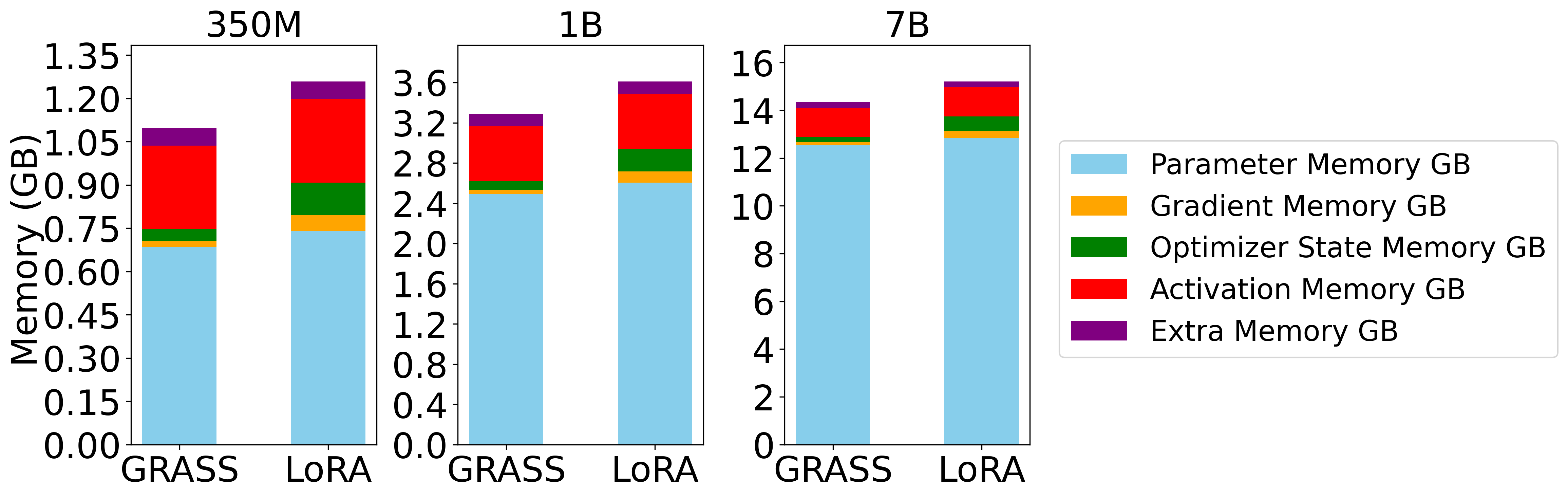
Figure 9: LLaMA finetuning memory footprint of Grass and LoRA for rank $r=64$, sequence length $256$, batch size $1$.

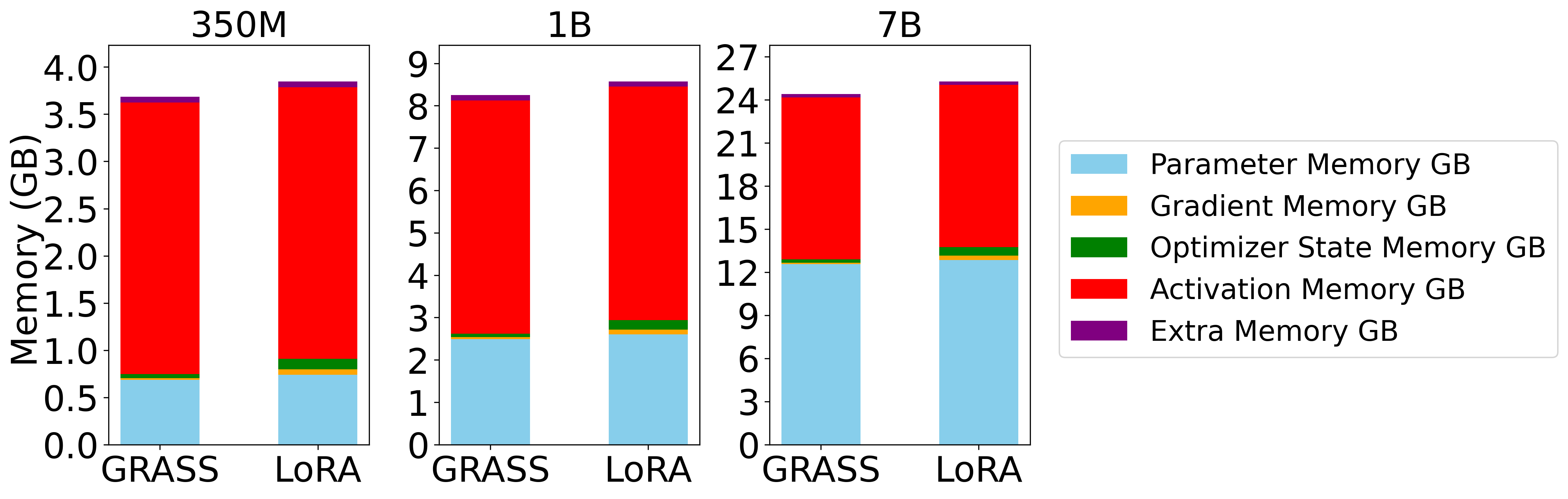
Figure 10: LLaMA finetuning memory footprint of Grass and LoRA for rank $r=64$, sequence length $512$, batch size $4$.

Appendix K Experiment: Finetuning Memory

In Figure 9 and Figure 10, we compare the finetuning memory footprint of Grass and LoRA when finetuning a LLaMA model at various scales (350M, 1B, 7B) using token batch sizes of 256 and 2048 (4$\times$512), respectively. Both methods are applied to all linear layers with a fixed rank of 64. Our analysis reveals that at larger batch sizes, activations predominantly contribute to the memory footprint, resulting in comparable memory usage between Grass and LoRA.

We estimate memory requirements for finetuning using the same aproach from Section J but only accounting for the gradients and optimizer states corresponding to the trainable (instead of all the) parameters. Furthermore, LoRA requires storing in addition to $X$ (the input to the layer), the activations corresponding to the low-rank input $XA$ to compute the gradient of $B$, where $A$ and $B$ are the low-rank adapters (Zhang et al., 2023). This results in an additional memory requirement for LoRA of $2BLr$ bytes per linear layer.

Appendix L Experiments: Throughput

Figure 11 compares the normalized pretraining throughput (using the Full model) of Grass and GaLore across 60M, 350M, and 1B model sizes. We find that the throughput advantage of Grass over GaLore and Full is $>25\%$ for the 1B model at rank 64. The throughput approaches that of the full model, as model size decreases or projection rank increases.

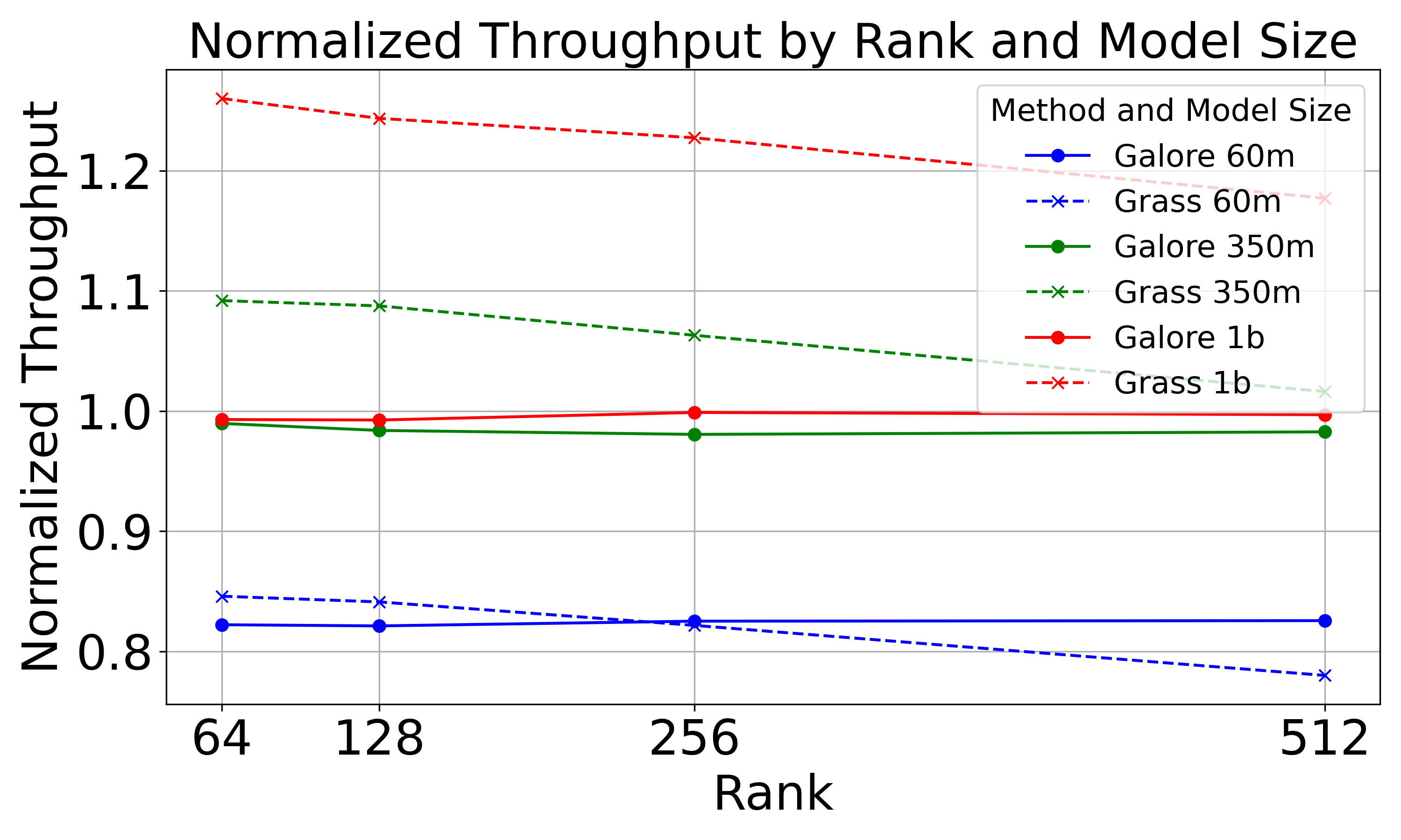
Figure 11: Rank vs Pretraining Throughput for Grass, LoRA and GaLore across 60M, 350M, 1B and 7B model sizes.

Figure 12: Rank vs LoRA Normalized Finetuning Throughput for Grass and GaLore across 60M, 350M, and 1B model sizes

Figure 12 compares the finetuning throughput across ranks 8, 16,32, and 64 for the Grass, GaLore, and LoRA baselines. For the ranks commonly used for finetuning (8-64) the throughput advantage of Grass remains about the same.

Appendix M Experiments: Additional Ablations

Comparison with other baselines

In Table 12, we report the validation perplexity of various other baselines on a LLaMA 1B pretraining task on the RealNews subset of C4. The attention and feedforward layers in all models are projected to a rank of 256, or use low rank adapters of this rank. We find that the training perplexities are lower while the validation perplexities are higher than in Table 5 for the 60M model due to overfitting on the RealNews dataset. All models use an update frequency of 200, and we tune the learning rate and scale factor $\alpha$ per model.

In addition to Grass and GaLore, we also include the ReLoRA baseline (Lialin et al., 2023) without any full-rank training warmup, the Flora baseline where $P$ has entries drawn from $\mathcal{N}(0,1/r)$, and the CountSketch baseline where $P^{\top}$ is a CountSketch matrix with $r$ rows with one nonzero entry from $\{\pm 1\}$ per column. The CountSketch projection has been previously applied to embedding layer gradients which are sparse in prior work (Spring et al., 2019), but shows larger variance and poorer convergence rates for dense gradients.

	Train Perp	Eval Perp
Full-Rank	33.48	31.41
Grass	33.52	32.17
GaLore	33.68	32.10
ReLoRA	34.30	34.19
Flora	35.91	35.62
CountSketch	36.97	36.93

Table 12: Comparison of various baselines using 1B LLaMA model validation perplexity. All models are pretrained on 500M tokens of the RealNews subset of C4. $r/d_{model}$ is 256/2048. Best baseline is bolded.

We see that Grass is competitive with GaLore, while ReLoRA, Flora, and CountSketch fall short. One way to interpret this is in terms of variance of the gradient sketches— Grass being data dependent and based on row norms can better approximate the gradient low rank subspace than a data agnostic sketch like Flora or CountSketch (Woodruff, 2014).

Grass with Adafactor

We pretrain the LLaMA 1B model with Grass and Full-rank in BF16 on the Realnews subset of C4 using the Adafactor optimizer (Shazeer and Stern, 2018) as an alternative to Adam for opt. Adafactor achieves sub-linear memory cost by factorizing the second-order statistics using a row-column outer product.

For Grass we use learning rate $0.005$, $\alpha=0.25$, $r=256$, $K=200$, batch size $512$, optimizer restart with a restart warmup of $100$ steps and no initial warmup. For Full-rank training, we use learning rate $0.0005$, batch size $512$, and $1000$ initial linear learning rate warmup steps.

In Figure 13 we report the train perplexity and see that Grass is within 1 perplexity point of Full-rank, demonstrating its ability to work with other inner off-the-shelf optimizers beyond Adam.

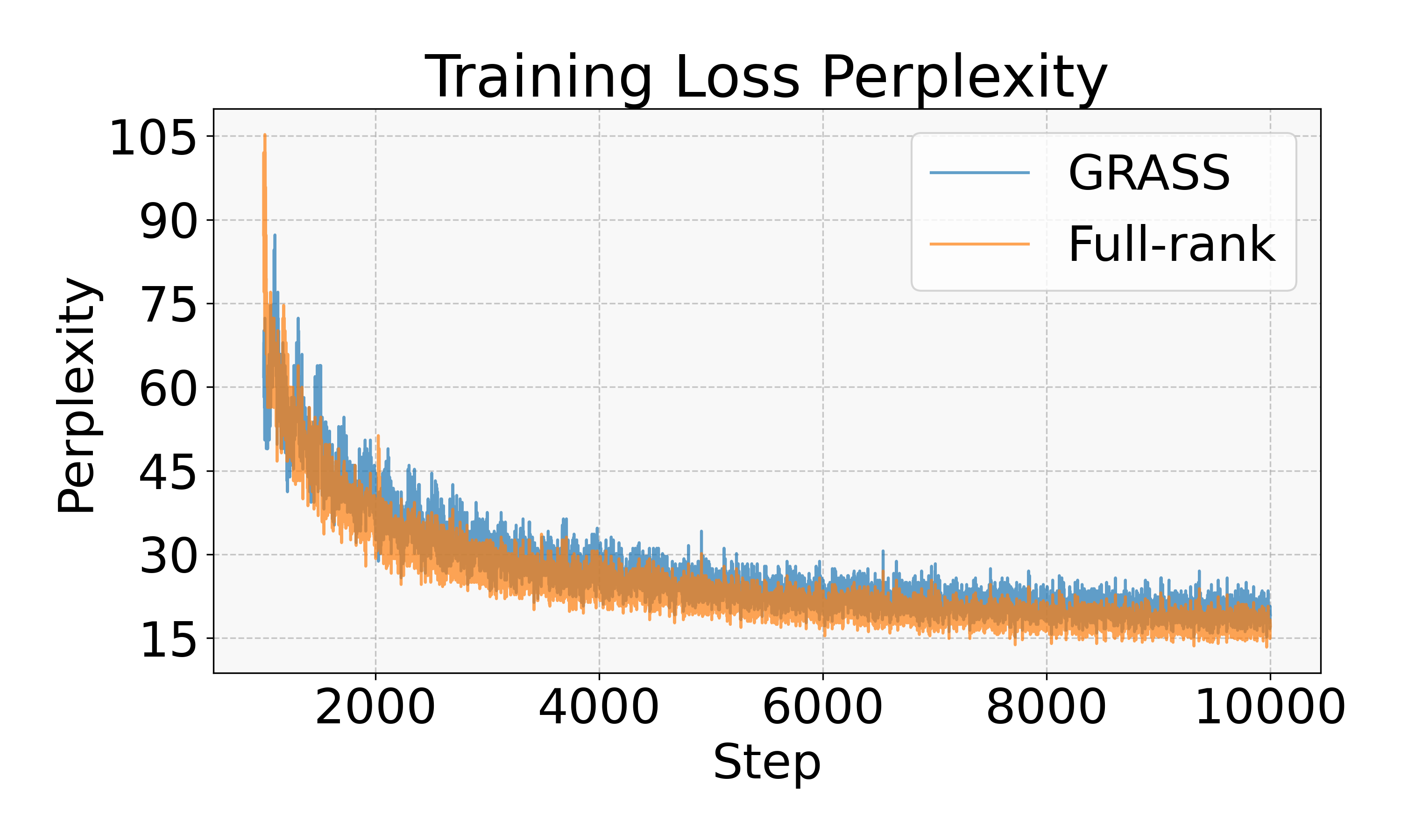
Figure 13: Pretraining LLaMA 1B on Realnews C4 subset with Adafactor.

Coverage of indices.

In Figure 14, we plot the coverage defined as the union of indices selected over $n$ update projection steps divided by the total indices per layer. We plot the coverage for the 60M LLaMA model pretrained on the C4 RealNews subset, for $n=15$ updates with $K=200$ steps between updates. Here, with the rank $128$ and the the number of rows $m=512$, a uniform sampling with replacement over 15 iterations should on average cover $1-\left(\left(1-\frac{1}{512}\right)^{128}\right)^{15}\approx 97.66\%$ of all the 512 indices in each layer. Empirically, all sampling methods exhibit good coverage with the Multinomial-Norm²-NR being close to uniform. Top-$r$ and Multinomial-Norm²-R oversample indices in certain layers, suggesting potential areas for further investigation into their utility in pruning strategies.

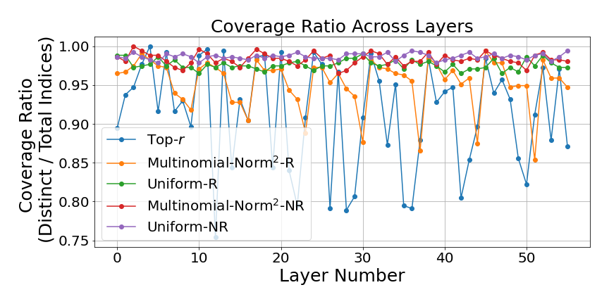
Figure 14: Per layer indices coverage (Distinct/Total) for the sampling strategies across 100 pretraining iterations.

In Figure 16 and Figure 16 we plot the aggregated sampled indices over 15 iterations of 60M LLaMA pretraining on the RealNews subset of C4. We see that while Multinomial-Norm²-NR and Top-$r$ attain similar performance in terms of perplexity, the sampled indices can be quite different, with Top-$r$ tending to oversample indices in particular layers.

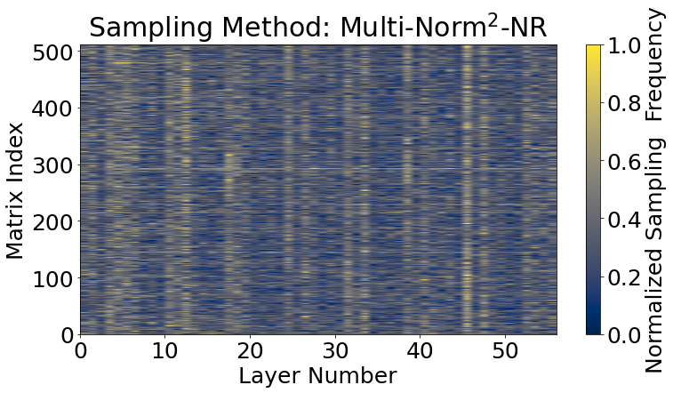
Figure 15: Multinomial-Norm² Sampling without Replacement: Heatmap of indices sampled for the different layers across 15 iterations of LLaMA 60M C4 pretraining.

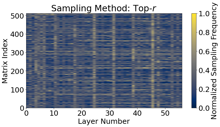
Figure 16: Top-$r$ Selection: Heatmap of indices sampled for the different layers across 15 iterations of LLaMA 60M C4 pretraining.

References

- Alistarh et al. (2017) Dan Alistarh, Demjan Grubic, Jerry Li, Ryota Tomioka, and Milan Vojnovic. 2017. Qsgd: Communication-efficient sgd via gradient quantization and encoding. In Advances in Neural Information Processing Systems, volume 30. Curran Associates, Inc.
- Anil et al. (2019) Rohan Anil, Vineet Gupta, Tomer Koren, and Yoram Singer. 2019. Memory efficient adaptive optimization. In Advances in Neural Information Processing Systems, volume 32. Curran Associates, Inc.
- Bernstein et al. (2018) Jeremy Bernstein, Yu-Xiang Wang, Kamyar Azizzadenesheli, and Animashree Anandkumar. 2018. signSGD: Compressed optimisation for non-convex problems. In Proceedings of the 35th International Conference on Machine Learning, volume 80 of Proceedings of Machine Learning Research, pages 560–569. PMLR.
- Biderman et al. (2024) Dan Biderman, Jose Gonzalez Ortiz, Jacob Portes, Mansheej Paul, Philip Greengard, Connor Jennings, Daniel King, Sam Havens, Vitaliy Chiley, Jonathan Frankle, Cody Blakeney, and John P. Cunningham. 2024. Lora learns less and forgets less. arXiv preprint arXiv: 2405.09673.
- Cer et al. (2017) Daniel Cer, Mona Diab, Eneko Agirre, Iñigo Lopez-Gazpio, and Lucia Specia. 2017. SemEval-2017 task 1: Semantic textual similarity multilingual and crosslingual focused evaluation. In Proceedings of the 11th International Workshop on Semantic Evaluation (SemEval-2017), pages 1–14, Vancouver, Canada. Association for Computational Linguistics.
- Chen et al. (2016) Tianqi Chen, Bing Xu, Chiyuan Zhang, and Carlos Guestrin. 2016. Training deep nets with sublinear memory cost. arXiv preprint arXiv: 1604.06174.
- Choquette et al. (2021) Jack Choquette, Wishwesh Gandhi, Olivier Giroux, Nick Stam, and Ronny Krashinsky. 2021. Nvidia a100 tensor core gpu: Performance and innovation. IEEE Micro, 41(2):29–35.
- Dettmers et al. (2021) Tim Dettmers, M. Lewis, Sam Shleifer, and Luke Zettlemoyer. 2021. 8-bit optimizers via block-wise quantization. International Conference on Learning Representations.
- Dettmers et al. (2023) Tim Dettmers, Artidoro Pagnoni, Ari Holtzman, and Luke Zettlemoyer. 2023. Qlora: Efficient finetuning of quantized llms. NEURIPS.
- Dolan and Brockett (2005) Bill Dolan and Chris Brockett. 2005. Automatically constructing a corpus of sentential paraphrases. In Third International Workshop on Paraphrasing (IWP2005). Asia Federation of Natural Language Processing.
- Gustafson (1988) John L. Gustafson. 1988. Reevaluating amdahl’s law. Commun. ACM, 31(5):532–533.
- Hao et al. (2024) Yongchang Hao, Yanshuai Cao, and Lili Mou. 2024. Flora: Low-rank adapters are secretly gradient compressors. arXiv preprint arXiv:2402.03293.
- Hendrycks et al. (2020) Dan Hendrycks, Collin Burns, Steven Basart, Andy Zou, Mantas Mazeika, D. Song, and J. Steinhardt. 2020. Measuring massive multitask language understanding. International Conference on Learning Representations.
- Hu et al. (2021) Edward J Hu, Yelong Shen, Phillip Wallis, Zeyuan Allen-Zhu, Yuanzhi Li, Shean Wang, Lu Wang, and Weizhu Chen. 2021. Lora: Low-rank adaptation of large language models. arXiv preprint arXiv:2106.09685.
- Kingma and Ba (2014) Diederik P Kingma and Jimmy Ba. 2014. Adam: A method for stochastic optimization. arXiv preprint arXiv:1412.6980.
- Levesque et al. (2012) Hector Levesque, Ernest Davis, and Leora Morgenstern. 2012. The winograd schema challenge. In Thirteenth international conference on the principles of knowledge representation and reasoning.
- Li et al. (2023) Bingrui Li, Jianfei Chen, and Jun Zhu. 2023. Memory efficient optimizers with 4-bit states. In Advances in Neural Information Processing Systems, volume 36, pages 15136–15171. Curran Associates, Inc.
- Lialin et al. (2023) Vladislav Lialin, Sherin Muckatira, Namrata Shivagunde, and Anna Rumshisky. 2023. ReloRA: High-rank training through low-rank updates. In Workshop on Advancing Neural Network Training: Computational Efficiency, Scalability, and Resource Optimization (WANT@NeurIPS 2023).
- Lin et al. (2018) Yujun Lin, Song Han, Huizi Mao, Yu Wang, and Bill Dally. 2018. Deep gradient compression: Reducing the communication bandwidth for distributed training. In 6th International Conference on Learning Representations, ICLR 2018, Vancouver, BC, Canada, April 30 - May 3, 2018, Conference Track Proceedings. OpenReview.net.
- Liu et al. (2019) Yinhan Liu, Myle Ott, Naman Goyal, Jingfei Du, Mandar Joshi, Danqi Chen, Omer Levy, Mike Lewis, Luke Zettlemoyer, and Veselin Stoyanov. 2019. Roberta: A robustly optimized bert pretraining approach. arXiv preprint arXiv: 1907.11692.
- Lv et al. (2023a) Kai Lv, Hang Yan, Qipeng Guo, Haijun Lv, and Xipeng Qiu. 2023a. Adalomo: Low-memory optimization with adaptive learning rate. arXiv preprint arXiv: 2310.10195.
- Lv et al. (2023b) Kai Lv, Yuqing Yang, Tengxiao Liu, Qinghui Gao, Qipeng Guo, and Xipeng Qiu. 2023b. Full parameter fine-tuning for large language models with limited resources. arXiv preprint arXiv: 2306.09782.
- Magdon-Ismail (2010) Malik Magdon-Ismail. 2010. Row sampling for matrix algorithms via a non-commutative bernstein bound. arXiv preprint arXiv: 1008.0587.
- Paszke et al. (2019) Adam Paszke, Sam Gross, Francisco Massa, Adam Lerer, James Bradbury, Gregory Chanan, Trevor Killeen, Zeming Lin, N. Gimelshein, L. Antiga, Alban Desmaison, Andreas Köpf, E. Yang, Zach DeVito, Martin Raison, A. Tejani, Sasank Chilamkurthy, Benoit Steiner, Lu Fang, Junjie Bai, and Soumith Chintala. 2019. Pytorch: An imperative style, high-performance deep learning library. Neural Information Processing Systems.
- Raffel et al. (2020) Colin Raffel, Noam Shazeer, Adam Roberts, Katherine Lee, Sharan Narang, Michael Matena, Yanqi Zhou, Wei Li, and Peter J. Liu. 2020. Exploring the limits of transfer learning with a unified text-to-text transformer. J. Mach. Learn. Res., 21:140:1–140:67.
- Raffel et al. (2019) Colin Raffel, Noam M. Shazeer, Adam Roberts, Katherine Lee, Sharan Narang, Michael Matena, Yanqi Zhou, Wei Li, and Peter J. Liu. 2019. Exploring the limits of transfer learning with a unified text-to-text transformer. J. Mach. Learn. Res., 21:140:1–140:67.
- Rajbhandari et al. (2020) Samyam Rajbhandari, Jeff Rasley, Olatunji Ruwase, and Yuxiong He. 2020. Zero: Memory optimizations toward training trillion parameter models. In SC20: International Conference for High Performance Computing, Networking, Storage and Analysis, pages 1–16.
- Rajpurkar et al. (2016) Pranav Rajpurkar, Jian Zhang, Konstantin Lopyrev, and Percy Liang. 2016. Squad: 100,000+ questions for machine comprehension of text. Conference on Empirical Methods in Natural Language Processing.
- Renggli et al. (2019) Cedric Renggli, Saleh Ashkboos, Mehdi Aghagolzadeh, Dan Alistarh, and Torsten Hoefler. 2019. Sparcml: high-performance sparse communication for machine learning. In Proceedings of the International Conference for High Performance Computing, Networking, Storage and Analysis, SC ’19, New York, NY, USA. Association for Computing Machinery.
- Seide et al. (2014) Frank Seide, Hao Fu, Jasha Droppo, Gang Li, and Dong Yu. 2014. 1-bit stochastic gradient descent and application to data-parallel distributed training of speech dnns. In Interspeech 2014.
- Shazeer (2020) Noam Shazeer. 2020. Glu variants improve transformer. arXiv preprint arXiv: 2002.05202.
- Shazeer and Stern (2018) Noam Shazeer and Mitchell Stern. 2018. Adafactor: Adaptive learning rates with sublinear memory cost. In International Conference on Machine Learning, pages 4596–4604. PMLR.
- Sheng et al. (2023) Ying Sheng, Shiyi Cao, Dacheng Li, Coleman Hooper, Nicholas Lee, Shuo Yang, Christopher Chou, Banghua Zhu, Lianmin Zheng, Kurt Keutzer, Joseph E. Gonzalez, and Ion Stoica. 2023. S-lora: Serving thousands of concurrent lora adapters. arXiv preprint arXiv: 2311.03285.
- Socher et al. (2013) Richard Socher, Alex Perelygin, Jean Wu, Jason Chuang, Christopher D. Manning, Andrew Ng, and Christopher Potts. 2013. Recursive deep models for semantic compositionality over a sentiment treebank. In Proceedings of the 2013 Conference on Empirical Methods in Natural Language Processing, pages 1631–1642, Seattle, Washington, USA. Association for Computational Linguistics.
- Soldaini et al. (2024) Luca Soldaini, Rodney Kinney, Akshita Bhagia, Dustin Schwenk, David Atkinson, Russell Authur, Ben Bogin, Khyathi Chandu, Jennifer Dumas, Yanai Elazar, Valentin Hofmann, Ananya Harsh Jha, Sachin Kumar, Li Lucy, Xinxi Lyu, Nathan Lambert, Ian Magnusson, Jacob Morrison, Niklas Muennighoff, Aakanksha Naik, Crystal Nam, Matthew E. Peters, Abhilasha Ravichander, Kyle Richardson, Zejiang Shen, Emma Strubell, Nishant Subramani, Oyvind Tafjord, Pete Walsh, Luke Zettlemoyer, Noah A. Smith, Hannaneh Hajishirzi, Iz Beltagy, Dirk Groeneveld, Jesse Dodge, and Kyle Lo. 2024. Dolma: an open corpus of three trillion tokens for language model pretraining research. arXiv preprint arXiv: 2402.00159.
- Spring et al. (2019) Ryan Spring, Anastasios Kyrillidis, Vijai Mohan, and Anshumali Shrivastava. 2019. Compressing gradient optimizers via count-sketches. International Conference on Machine Learning.
- Stich et al. (2018) Sebastian U Stich, Jean-Baptiste Cordonnier, and Martin Jaggi. 2018. Sparsified sgd with memory. In Advances in Neural Information Processing Systems, volume 31. Curran Associates, Inc.
- Tang et al. (2021) Hanlin Tang, Shaoduo Gan, Ammar Ahmad Awan, Samyam Rajbhandari, Conglong Li, Xiangru Lian, Ji Liu, Ce Zhang, and Yuxiong He. 2021. 1-bit adam: Communication efficient large-scale training with adam’s convergence speed. In Proceedings of the 38th International Conference on Machine Learning, volume 139 of Proceedings of Machine Learning Research, pages 10118–10129. PMLR.
- Taori et al. (2023) Rohan Taori, Ishaan Gulrajani, Tianyi Zhang, Yann Dubois, Xuechen Li, Carlos Guestrin, Percy Liang, and Tatsunori B. Hashimoto. 2023. Stanford alpaca: An instruction-following llama model. https://github.com/tatsu-lab/stanford_alpaca.
- Touvron et al. (2023) Hugo Touvron, Louis Martin, Kevin Stone, Peter Albert, Amjad Almahairi, Yasmine Babaei, Nikolay Bashlykov, Soumya Batra, Prajjwal Bhargava, Shruti Bhosale, Dan Bikel, Lukas Blecher, Cristian Canton Ferrer, Moya Chen, Guillem Cucurull, David Esiobu, Jude Fernandes, Jeremy Fu, Wenyin Fu, Brian Fuller, Cynthia Gao, Vedanuj Goswami, Naman Goyal, Anthony Hartshorn, Saghar Hosseini, Rui Hou, Hakan Inan, Marcin Kardas, Viktor Kerkez, Madian Khabsa, Isabel Kloumann, Artem Korenev, Punit Singh Koura, Marie-Anne Lachaux, Thibaut Lavril, Jenya Lee, Diana Liskovich, Yinghai Lu, Yuning Mao, Xavier Martinet, Todor Mihaylov, Pushkar Mishra, Igor Molybog, Yixin Nie, Andrew Poulton, Jeremy Reizenstein, Rashi Rungta, Kalyan Saladi, Alan Schelten, Ruan Silva, Eric Michael Smith, Ranjan Subramanian, Xiaoqing Ellen Tan, Binh Tang, Ross Taylor, Adina Williams, Jian Xiang Kuan, Puxin Xu, Zheng Yan, Iliyan Zarov, Yuchen Zhang, Angela Fan, Melanie Kambadur, Sharan Narang, Aurelien Rodriguez, Robert Stojnic, Sergey Edunov, and Thomas Scialom. 2023. Llama 2: Open foundation and fine-tuned chat models. arXiv preprint arXiv: 2307.09288.
- Vogels et al. (2019) Thijs Vogels, Sai Praneeth Karimireddy, and Martin Jaggi. 2019. Powersgd: Practical low-rank gradient compression for distributed optimization. In Advances in Neural Information Processing Systems, volume 32. Curran Associates, Inc.
- Wang et al. (2018a) Alex Wang, Amanpreet Singh, Julian Michael, Felix Hill, Omer Levy, and Samuel R. Bowman. 2018a. Glue: A multi-task benchmark and analysis platform for natural language understanding. BLACKBOXNLP@EMNLP.
- Wang et al. (2018b) Hongyi Wang, Scott Sievert, Shengchao Liu, Zachary Charles, Dimitris Papailiopoulos, and Stephen Wright. 2018b. Atomo: Communication-efficient learning via atomic sparsification. Advances in neural information processing systems, 31.
- Wang et al. (2023) Yizhong Wang, Hamish Ivison, Pradeep Dasigi, Jack Hessel, Tushar Khot, Khyathi Raghavi Chandu, David Wadden, Kelsey MacMillan, Noah A. Smith, Iz Beltagy, and Hannaneh Hajishirzi. 2023. How far can camels go? exploring the state of instruction tuning on open resources. Neural Information Processing Systems.
- Warstadt et al. (2018) Alex Warstadt, Amanpreet Singh, and Samuel R. Bowman. 2018. Neural network acceptability judgments. Transactions of the Association for Computational Linguistics.
- Wei et al. (2021) Jason Wei, Maarten Bosma, Vincent Y. Zhao, Kelvin Guu, Adams Wei Yu, Brian Lester, Nan Du, Andrew M. Dai, and Quoc V. Le. 2021. Finetuned language models are zero-shot learners. arXiv preprint arXiv: 2109.01652.
- Wen et al. (2017) Wei Wen, Cong Xu, Feng Yan, Chunpeng Wu, Yandan Wang, Yiran Chen, and Hai Li. 2017. Terngrad: Ternary gradients to reduce communication in distributed deep learning. In Advances in Neural Information Processing Systems, volume 30. Curran Associates, Inc.
- Williams et al. (2017) Adina Williams, Nikita Nangia, and Samuel R. Bowman. 2017. A broad-coverage challenge corpus for sentence understanding through inference. arXiv preprint arXiv: 1704.05426.
- Woodruff (2014) David P. Woodruff. 2014. Sketching as a tool for numerical linear algebra. Foundations and Trends® in Theoretical Computer Science.
- Xia et al. (2024) Wenhan Xia, Chengwei Qin, and Elad Hazan. 2024. Chain of lora: Efficient fine-tuning of language models via residual learning. arXiv preprint arXiv: 2401.04151.
- Zhang and Sennrich (2019) Biao Zhang and Rico Sennrich. 2019. Root mean square layer normalization. In Advances in Neural Information Processing Systems, volume 32. Curran Associates, Inc.
- Zhang et al. (2023) Longteng Zhang, Lin Zhang, Shaohuai Shi, Xiaowen Chu, and Bo Li. 2023. Lora-fa: Memory-efficient low-rank adaptation for large language models fine-tuning. arXiv preprint arXiv: 2308.03303.
- Zhao et al. (2024) Jiawei Zhao, Zhenyu Zhang, Beidi Chen, Zhangyang Wang, Anima Anandkumar, and Yuandong Tian. 2024. Galore: Memory-efficient llm training by gradient low-rank projection. arXiv preprint arXiv:2403.03507.