Density-Based Long-Range Electrostatic Descriptors
for Machine Learning Force Fields

Abstract

This study presents a long-range descriptor for machine learning force fields (MLFFs) that maintains translational and rotational symmetry, similar to short-range descriptors while being able to incorporate long-range electrostatic interactions. The proposed descriptor is based on an atomic density representation and is structurally similar to classical short-range atom-centered descriptors, making it straightforward to integrate into machine learning schemes. The effectiveness of our model is demonstrated through comparative analysis with the long-distance equivariant (LODE) (Grisafi and Ceriotti, 2019) descriptor. In a toy model with purely electrostatic interactions, our model achieves errors below 0.1%.
The application of our descriptors, in combination with local descriptors representing the atomic density, to materials where monopole-monopole interactions are important such as sodium chloride successfully captures long-range interactions, improving predictive accuracy. The study highlights the limitations of the combined LODE method in materials where intermediate-range effects play a significant role. Our work presents a promising approach to addressing the challenge of incorporating long-range interactions into MLFFs, which enhances predictive accuracy for charged materials to the level of state-of-the-art Message Passing Neural Networks.

I Introduction

Machine learning force fields (MLFFs) are a powerful tool for accurately and efficiently predicting inter-atomic potentials, approaching the precision of ab-initio calculations (Manzhos and Carrington, 2006; Behler and Parrinello, 2007; Bartók et al., 2010; Rupp et al., 2012; Behler, 2015; Thompson et al., 2015; Morawietz et al., 2016; Bartók et al., 2018; Schütt et al., 2018; Deringer, Caro, and Csányi, 2019; Drautz, 2019; von Lilienfeld, Müller, and Tkatchenko, 2020; von Lilienfeld and Burke, 2020; Unke et al., 2021a; Keith et al., 2021; Batzner et al., 2022; Batatia et al., 2022; Ko and Ong, 2023; Merchant et al., 2023; Batatia et al., 2023). MLFFs describe the potential energy as a function of descriptors that represent the atomic structure of a given material.
To increase the efficiency of MLFFs, many methods rely on a local descriptor that solely represents the atomic environment in the vicinity of an atom within a specified cutoff sphere. These methods assume that all interactions between atoms further apart than the cutoff radius are negligible. While this approach accurately describes many materials and their properties, it neglects long-range interactions such as electrostatics. This is because, in practice, it is impossible to arbitrarily increase the cutoff radius. However, these long-range interactions can be important Kjellander (2018); Guo et al. (2018); Jorn et al. (2013); French et al. (2010), and new methods that include long-range interactions are necessary to improve the predictive power of MLFFs for systems with long-range electrostatics Ko et al. (2021); Unke et al. (2021b); Ambrosetti et al. (2016); Stöhr and Tkatchenko (2019); Unke et al. (2022).

This issue is widely recognized, and various methods have been developed to address it. Recent models have concentrated on specific types of long-range interactions, such as electrostatics, and have introduced correction terms to account for them Grisafi and Ceriotti (2019); Grisafi, Nigam, and Ceriotti (2021); Ko et al. (2021); Unke et al. (2021b); Zhang et al. (2022); Bereau et al. (2018); Yao et al. (2018); Unke and Meuwly (2019); Niblett, Galib, and Limmer (2021); Gao and Remsing (2022). A common approach is to split the energy into distinct parts and model them independently. Then, all contributions are added together to calculate the total energy. Short-range contributions are typically calculated with a local model, while long-range components are modeled with diverse approaches. One can either treat the various energy terms separately and train two machine learning (ML) models, adding up the final energies, or utilize combined descriptors and train a single model.
Many of these methods use classical (non-equivariant and or even non-message passing) neural networks (NNs)Ko et al. (2021); Zhang et al. (2022); Yao et al. (2018); Unke and Meuwly (2019); Niblett, Galib, and Limmer (2021); Gao and Remsing (2022), or kernel methods Grisafi and Ceriotti (2019); Grisafi, Nigam, and Ceriotti (2021); Bereau et al. (2018); Huguenin-Dumittan et al. (2023). Deep NNs offer more flexibility but require more data for training and are generally slow to train. Kernel methods are more convenient for small to medium-sized problems, as they can rely on dense linear algebra routines to solve the linear least squares problem Bishop (2010).

Another approach to include long-range interactions is to use short-range descriptors, but effectively propagate interactions beyond the distinct cutoff by employing Message Passing Neural Networks (MPNNs) Gilmer et al. (2017); Schütt et al. (2018); Bronstein et al. (2021); Unke et al. (2021b); Batzner et al. (2022); Batatia et al. (2022); Haghighatlari et al. (2022); Gasteiger, Groß, and Günnemann (2022); Takamoto, Izumi, and Li (2022); Chen and Ong (2022); Deng et al. (2023); Merchant et al. (2023); Batatia et al. (2023). Equivariant MPNNs such as NewtonNet Haghighatlari et al. (2022), DimeNet Gasteiger, Groß, and Günnemann (2022), TeaNet Takamoto, Izumi, and Li (2022), NequIP Batzner et al. (2022) and MACE Batatia et al. (2022) offer unique advantages due to their specialized architectures.
NewtonNet is designed to respect Newtonian mechanics, ensuring that the learned forces obey physical laws. It also incorporates directional information from forces, enhancing the model’s accuracy Haghighatlari et al. (2022). DimeNet employs directional message passing, which allows it to capture complex interactions effectively Gasteiger, Groß, and Günnemann (2022). TeaNet uses tensor-based message passing, facilitating the learning of intricate relationships between atomic structures Takamoto, Izumi, and Li (2022).
NequIPBatzner et al. (2022) employs equivariant convolutions of tensorial quantities, resulting in a particularly flexible network topology with many millions of parameters. MACE Batatia et al. (2022) is in most respects a simplified version of NequIP usually relying on only two message-passing layers and largely linear activation functions. This should improve execution speed and learning efficiency.

This work utilizes kernel methods. Our objective is to find a physically meaningful and flexible approach for describing long-range interactions without resorting to a global and non-atom-centered description. We present a new descriptor encoding the atomic density. The atomic density is described similarly to short-range models Jinnouchi, Karsai, and Kresse (2019); Jinnouchi et al. (2019, 2020a, 2020b). However, we implicitly account for all periodic images of all atoms in the supercell by treating the atomic density in reciprocal space.
This approach offers the advantage of a flexible, physics-based descriptor that is atom-centered but also long-ranged. It can be easily combined with a local descriptor, as both have the same mathematical form, albeit in its present implementation it is not yet very performant.
We apply the new approach to a gas of point charges. The descriptor is then compared to the long-distance equivariant (LODE) framework Grisafi and Ceriotti (2019) and the MPNN MACE Batatia et al. (2022) for liquid sodium chloride and zirconia.

II Theory

II.1 Short-Range Descriptors

The descriptors used in this work are designed to resemble the density-based Smooth Overlap of Atomic Positions (SOAP) Bartók et al. (2010) and Gaussian Approximation Potential (GAP) Bartók, Kondor, and Csányi (2013) descriptors. The atomic density $\rho$ is calculated around each atom $j$ as a function of the atomic positions denoted as r. The expansion coefficients

$$c_{nlm}^{jJ}=\sum_{k=1}^{N_{J}}h_{nl}\left(r_{jk}\right)Y_{lm}^{*}\left(\hat{\textbf{r}}_{jk}\right)$$ (1)

with

$$h_{nl}\left(r\right) =\frac{4\pi}{\left(\sqrt{2\sigma^{2}\pi}\right)^{3}}f_{\text{cut}}\left(r\right)\int_{0}^{\infty}\chi_{nl}\left(r^{\prime}\right)$$ (2)

$$\times\exp\left(-\frac{r^{\prime 2}+r^{2}}{2\sigma^{2}}\right)\iota_{l}\left(\frac{rr^{\prime}}{\sigma^{2}}\right)r^{\prime 2}\text{d}r^{\prime}$$ (3)

from Jinnouchi, Karsai, and Kresse (2019) that are given there in Eq. (18) and (19) are used for building the short-range descriptors. Here, the vector $\textbf{r}_{jk}$ is the vector pointing from atom $j$ to $k$, $\textbf{r}_{k}-\textbf{r}_{j}$. The set of radial $\chi_{nl}$ and angular $Y_{lm}$ basis functions are used to expand the atomic density in order to obtain rotational and translational invariant expansion coefficients Bartók et al. (2010); Bartók, Kondor, and Csányi (2013). The indices $l$, $m$, and $n$ are the angular, momentum, and radial index, respectively. The parameter $\sigma$ is used to broaden the density distribution. $\iota_{l}$ are the modified spherical Bessel functions of the first kind, and $N_{J}$ is the number of atoms of type $J$. The cutoff function $f_{\text{cut}}$ is used to ensure a smooth decay of $h_{nl}$ to zero at the cutoff radius.

The final descriptor $\textbf{X}_{j}$ describing the local environment surrounding atom $j$ is derived by combining the invariant ($l=0$) two-body expansion coefficients

$$c^{jJ}_{n}=c^{jJ}_{n00}$$ (4)

and the rotational and translational invariant three-body expansion coefficients

$$p^{jJJ^{\prime}}_{nn^{\prime}l}=\sqrt{\frac{8\pi^{2}}{2l+1}}\sum_{m=-l}^{l}c^{jJ}_{nlm}c^{jJ^{\prime}}_{n^{\prime}lm}$$ (5)

into vectors

$$\textbf{X}_{j}^{(2)} =\left(c^{i1}_{1},c^{i1}_{2},\ldots,c^{i2}_{1},c^{i2}_{2},\ldots\right)^{T}$$ (6)

$$\textbf{X}_{j}^{(3)} =\left(p^{i11}_{110},p^{i11}_{111},\ldots,p^{i11}_{120},p^{i11}_{121},\ldots,p^{i12}_{110},\ldots,p^{i22}_{110},\ldots\right)^{T}$$ (7)

that are then combined to

$$\textbf{X}_{j}=\begin{pmatrix}\beta^{(2)}\textbf{X}_{j}^{(2)}\\ \beta^{(3)}\textbf{X}_{j}^{(3)}\end{pmatrix}$$ (8)

using the weights $\beta$ for the two- and three-body descriptors. In the present calculations $\beta^{(2)}=\sqrt{0.1}$ and $\beta^{(3)}=\sqrt{0.9}$ were used for the short-range descriptors. Whenever inproducts are formed in the kernel, the weights are implicitly squared, so this results in a metric with "weights" of 0.1 and 0.9 for two-body and three-body terms.

II.2 Long-Range Descriptors

The objective is to calculate a similar set of descriptors where the expansion coefficients however represent the atomic density over long ranges and multiple supercells. The same ansatz as in real space is used, where the expansion coefficients are designed to represent the atomic density. As before, the descriptors are obtained by projecting the density onto a product basis of radial and angular functions. However, to avoid introducing a cutoff, the corresponding products are evaluated in reciprocal instead of real space:

$$c_{nlm}^{jJ}=\sum_{k=1}^{N_{J}}\sum_{\textbf{G}}\exp\left(i\textbf{G}\left(\textbf{r}_{k}-\textbf{r}_{j}\right)\right)\exp\left(-\frac{|\textbf{G}|^{2}\sigma^{2}}{2}\right)f_{nlm}^{*}(\textbf{G})$$ (9)

where G are momentum vectors consistent with the periodic boundary conditions, and $f_{nlm}(\textbf{G})$ are the basis functions in reciprocal space and the other terms represent the broadened atomic density distribution of atom $k$ of type $J$ with positions $\textbf{r}_{k}$ around atom $j$ with positions $\textbf{r}_{j}$. The central atom $j$ may be of any atom type present in the material. This allows for the inclusion of interactions between atoms of different types in the descriptor.
Starting out from the product of the radial $\chi_{nl}\left(r\right)$ and angular $Y_{lm}\left(\hat{\textbf{r}}\right)$ basis functions in real space

$$f_{nlm}(\textbf{r})=\chi_{nl}\left(r\right)Y_{lm}\left(\hat{\textbf{r}}\right)$$ (10)

taking the Fourier Transform (FT) of Eq. (10) and applying the plane wave expansion yields

$$f_{nlm}(\textbf{G})=4\pi i^{l}Y_{lm}(-\hat{\textbf{G}})\int_{0}^{\infty}r^{2}j_{l}(\textbf{G}r)\chi_{nl}(r)\text{d}r$$ (11)

where the remaining integral can be either solved analytically or numerically depending on the choice of radial basis functions $\chi_{nl}(r)$.

The long-range expansion coefficients given in Eq. (9) have the same form as the short-range expansion coefficients given in Eq. (1), but with the appropriate choice of basis functions (see next section), they can encode the long-range density. This is due to the calculation in reciprocal space, where not only the position of an atom is considered but also all periodic images of this atom. It is important to note that these long-range descriptors do not require a cutoff, but of course, it is possible to impose a cutoff by using the FT of finite-ranged real-space functions in Eq. (11).
The individual long-range expansion coefficients are then combined into a vector ("long-range descriptor"). We use only two-body expansion coefficients as shown in Eq. (4) and the corresponding vector $\textbf{X}_{j}^{(2)}$. The three-body long-range coefficients are excluded since the objective here is to describe long-range pairwise interactions. Furthermore, we found no improvements when including long-range three-body terms in any of the systems considered here. This might have many reasons, but we believe that three-body interactions are generally shorter-ranged. Consider, for instance, the case of Van der Waals (vdW) interactions: two-body vdW interactions fall off like $1/r^{6}$, and the three-body terms (Axilrod–Teller) fall off like $1/r^{9}$. Furthermore, three-body electrostatic interactions do not exist, as the Coulomb interaction is strictly two-body in nature.

II.3 Long-Range Radial Basis Functions

The type of basis functions used for the descriptors has not been specified yet. For the short-range method, spherical Bessel functions are used for the radial part and spherical harmonics for the angular part.
Spherical harmonics are also used for the angular part of the long-range descriptor. However, spherical Bessel functions cannot be employed to model the infinitely ranged interactions in the radial part. To maintain a fixed spatial resolution, the number of Bessel functions would need to increase with $R_{\text{cut}}$ and therefore go to infinity.
Given the objective of representing electrostatic interactions that decay slowly with $1/r$, where $r$ is the distance between two atoms, it is evident that exponentially decaying functions are a natural choice. This is because

$$\begin{split}\frac{1}{r}&=\int_{0}^{\infty}\exp(-\zeta r)\text{d}\zeta\\ &\approx\sum_{n=1}^{N_{\text{max}}}w_{n}\exp(-\zeta_{n}r)\end{split}$$ (12)

holds. The first line of Eq. (12) is the Laplace transform of $1/r$, while the second line approximates this integral using a quadrature rule. This demonstrates that the integral over all exponentially decaying functions can represent $1/r$, a fact that has been amply used in quantum chemistry to deal with integrals in many-body perturbation theory Häser and Almlöf (1992); Izmaylov and Scuseria (2008); Doser, Lambrecht, and Ochsenfeld (2008); Ayala and Scuseria (1999); Kaltak, Klimes, and Kresse (2014). However, it is necessary to determine the exponents $\zeta_{n}$ and $N_{\text{max}}$. We define $\zeta_{n}$ on a logarithmic mesh where

$$\zeta_{n}=\zeta_{\text{max}}/s^{n-1},$$ (13)

and $\zeta_{\text{max}}$ and the scaling constant $s$ are hyperparameters determined numerically. We note that for many-body applications a roughly exponential scaling was also found to be optimal, although we had rigorous procedures for determining an optimal scaling Kaltak, Klimes, and Kresse (2014). Those prescriptions are not easily adaptable to machine learning, though.

II.4 The LODE Implementation

Grisafi and Ceriotti introduced the long-distance equivariant (LODE) framework, which uses descriptors to encode the electrostatic potential around atoms Grisafi and Ceriotti (2019). The potential is calculated by summing the potentials induced by other atoms at the position of the central atom.
In reciprocal space, the electrostatic potential $\Phi$ is given as the negative product of the atomic density $\rho$ and the Coulomb Kernel

$$\Phi(\textbf{G})=-\frac{4\pi}{\|\textbf{G}\|^{2}\Omega}\rho(\textbf{G}).$$ (14)

where $\Omega$ is the volume of the supercell.
Because of the relation shown in Eq. (14), it is relatively easy, with the density-based model presented above, to implement the LODE descriptors as well. The only required step is to multiply the density-based expansion coefficients by the negative Coulomb kernel before summing over the reciprocal grid points G.
As in the original work of Grisafi and Ceriotti for real materials, the LODE descriptors are combined with short-range descriptors as well, using the approach shown in the following section.

II.5 Combination of Short- and Long-Range Descriptors

To apply the long-range models to realistic materials in which both short-range and long-range interactions are present, the final descriptor vectors X must contain information about both types of interaction. By simply appending the short-range descriptors $\textbf{X}_{\text{sr}}$ and long-range descriptors $\textbf{X}_{lr}$ the final descriptor

$$\textbf{X}=\left[\textbf{X}_{\text{sr}}^{T},\textbf{X}_{\text{lr}}^{T}\right]^{T}$$ (15)

is obtained. This descriptor contains all the necessary information and still provides a unique similarity measure for kernel-ridge regression.
It should be noted that no additional weighting for the short- and long-range descriptors is introduced here when combining them, as this was found the change the learning efficiency very little.

II.6 The Fitting Process

The fitting process of our model employs the methods of polipy4vasp, the code used in Ref. Schmiedmayer and Kresse (2024). These methods are implemented analogously to those of the Vienna Ab initio Simulation Package (VASP) Kresse and Furthmüller (1996a, b); Kresse and Joubert (1999) which are presented in Jinnouchi, Karsai, and Kresse (2019); Jinnouchi et al. (2019, 2020a).
The following paragraphs provide a brief overview of the main points of the scheme. It is assumed that there is a non-linear functional mapping of the final descriptors obtained as described above to the total energy of the system. As usual, it is furthermore assumed that the energy $U$ of the system can be decomposed into the sum

$$U=\sum_{j}U_{j}$$ (16)

of local energy contributions $U_{j}$ that depend on the "local" environment around each atom $j$. Kernel regression is used to describe the non-linear dependence of the energy on the descriptors. Either a Gaussian (radial basis function) kernel

$$K(\textbf{X}_{j},\textbf{X}_{b})=\text{exp}\left(-\frac{\|\textbf{X}_{j}-\textbf{X}_{b}\|^{2}}{\eta^{2}}\right)$$ (17)

or a polynomial kernel

$$K(\textbf{X}_{j},\textbf{X}_{b})=\left(\hat{\textbf{X}}_{j}\cdot\hat{\textbf{X}}_{b}\right)^{\zeta}$$ (18)

is used here.
In Eq. (18) $\hat{\textbf{X}}$ indicates that the descriptor X is normalized. The index $b$ in both Eq. (17) and Eq. (18) refers to the kernel basis function to which the descriptor of the current central atom $\textbf{X}_{j}$ is compared.

The energy per atom of structure $s$ containing $N_{\text{atom}}$ atoms is obtained when the following equation is fulfilled in the least squares sense:

$$\frac{U^{s}}{N_{\text{atom}}^{s}}\stackrel{{\scriptstyle!}}{{=}}\sum_{j=1}^{N_{\text{atom}}^{s}}\frac{U_{j}}{N_{\text{atom}}^{s}}=\sum_{b=1}^{N_{\text{b}}}w_{b}\sum_{j=1}^{N_{\text{atom}}^{s}}\frac{K(\textbf{X}_{j}^{s},\textbf{X}_{b})}{N_{\text{atom}}^{s}}.$$ (19)

Here $U^{s}$ is the energy of structure $s$ obtained from first principles (FP) calculations and $N_{b}$ is the total number of kernel basis functions. The energy $U^{s}$ is a linear function of the fitting weights $w_{b}$. As the forces are the negative derivatives of the energy with respect to the atomic positions, also the forces are linear functions of the weights $w_{b}$.
These linear relations can be expressed as a system of linear equations in matrix-vector form:

$$\textbf{y}\stackrel{{\scriptstyle!}}{{=}}\bm{\Phi}\textbf{w}.$$ (20)

The vector y contains the energies of all training structures $s$ and all the forces acting on all atoms in the systems included in the training data set obtained from FP calculations. These entries are made dimensionless by dividing them by the standard deviation of those energies and the forces, respectively.
During training the linear system of equations is solved using singular value decomposition, and singular values smaller than a threshold of $10^{-9}$ times the largest singular value are disposed of.

II.7 The Root-Mean Square Percentage Error

In this work, all errors of training and test data are given in terms of the root-mean-square percentage error (RMSPE). This is calculated by dividing the root-mean-square error of the predicted properties by the standard deviation of the exact results multiplied by $100$. With this approach, we obtain a unitless measure that does not depend on the number of atoms or the size of the unit cell. Typically, errors are given in (m)eV/atom for the energies and in eV/Å for the forces. However, these errors cannot be easily compared between different materials or at different temperatures. The RMSPE simplifies such comparisons.

III Results

For LODE the model with only pairwise descriptors and a body order term of $\nu=1$ is used. This facilitates a comparison with the purely radial description of the density-based long-range descriptors. Furthermore, it was found that the use of three-body terms in our case leads to higher errors compared to the use of only two-body terms. This is likely related to the already discussed two-body nature of long-range Coulomb interactions.

III.1 Long-Range Effects of Point Charges

As an initial test set for the present long-range model, a gas of randomly distributed point charges, analogous to the one used in Grisafi and Ceriotti (2019), was constructed. The set comprises systems of varying volumes, each containing 64 atoms, with 32 having a positive charge of $+1$ and the other 32 having a negative charge of $-1$. To prevent large energies the minimum distance between two atoms was set to $2.5$ Å. The training and validation data were generated using the Ewald energies and forces from VASP. Only long-range descriptors were used for this system.
For all tests on this toy model the Gaussian kernel given in Eq. (17) with a broadening of $\eta=1.55$ was used.

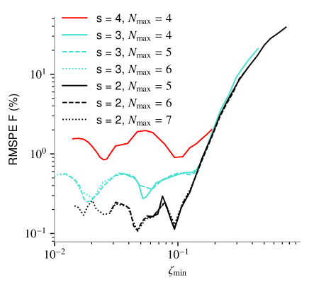
Figure 1: The RMSPE in the forces for various values of the minimal $\zeta_{\text{min}}=\zeta_{\text{max}}/s^{N_{\text{max}}-1}$ of the radial basis functions, scaling constants $s$, and number of radial basis functions $N_{\text{max}}$ for the gas of point charges. It is evident that the error reduction is primarily associated with a decreasing scaling constant. All curves with a small scaling constant of $s=2$ yield a minimum at $\zeta_{\text{min}}\approx 0.09$. Exponents larger than the minimum value are insufficiently long-ranged to accurately capture long-range electrostatic interactions.

The first step is to determine the radial basis functions. This involves optimizing three parameters: the number of radial basis functions $N_{\text{max}}$, the maximal exponent $\zeta_{\text{max}}$, and the scaling constant $s$. A grid search of these parameters was performed.
Figure 1 shows the minimal exponents $\zeta_{\text{min}}=\zeta_{\text{max}}/s^{N_{\text{max}}-1}$ on the x-axis and the corresponding error in the force predictions on the y-axis. Each line represents a distinct set of maximal exponents, $\zeta_{\text{max}}$, ranging from $12$ to $0.9$ and is associated with a specific value of $N_{\text{max}}$ and $s$. The linestyle and color of the lines indicate the value of $N_{\text{max}}$ and $s$, respectively.

Overall, reducing the scaling constant $s$ reduces the RMSPE. This is because a smaller scaling constant results in a denser distribution of radial basis functions, allowing for better a description of the electrostatic kernel ($1/r$). For the electrostatic interactions to be accurately described, it is necessary to have a sufficient number of basis functions such that they decay sufficiently slowly. We see a more or less pronounced minimum around $\zeta_{\text{min}}\approx 0.09$. The second minimum to the left corresponds to the case that the second smallest $\zeta$ becomes approximately $0.09$. For $\zeta$, the inclusion of values smaller than $0.09$ is unnecessary but also does not significantly degrade the quality of the fit.
The plot shows a steep increase in error on the right-hand side, indicating that the smallest exponent is insufficient to capture long-range electrostatic interactions. This occurs when the radial basis function with the smallest exponent decays too quickly and the basis functions are unable to model the long-range interactions.

We found that with a scaling constant of $s=2$ and 6 radial basis functions, relative errors of approximately $0.1$% are achieved.
The values $N_{\text{max}}=6$, $s=2$ and $\zeta_{\text{max}}=2$ are the optimal choices among all possible values for the density-based descriptors for the gas of point charges. These hyperparameters will be used in the subsequent calculations. Similar tests must be conducted to determine the optimal set of these three hyperparameters for other materials. However, the values obtained here provide a good starting point, which can help avoid extensive grid searches.

Next, we compare our approach with the LODE method, which is implemented in the way presented in II.4. It is known from theory that the two-body LODE descriptor is ideal for a system where only Coulomb interactions are present Grisafi and Ceriotti (2019). Consequently, using only two-body descriptors and a single radial basis function for a small cutoff is sufficient. In this case one descriptor for each interaction pair (+1, +1), (+1, -1), (-1, +1), and (-1, -1) suffices, as these exactly represent the interaction of one positive or negative point charge with all other positive or negative point charges. In our case, the radial basis function, onto which the charge is projected, is a spherical Bessel function that is smoothly cut off at the cutoff radius.
The density-based descriptors are not optimal for this case, so we need to use more radial basis functions and expansion coefficients to learn the Coulomb interactions. However, learning only pairwise interactions is sufficient even using density-based descriptors.

Figure 2 shows the learning curves for the two different methods. The LODE method was tested with various combinations of cutoff radii $R_{\text{cut}}$ and the number of radial basis functions $N_{\text{max}}$, resulting in different numbers of expansion coefficients, and potentially probing the electrostatic potentials at points further away from the central atom. For the LODE model, this adds irrelevant information for the simple point charge model.

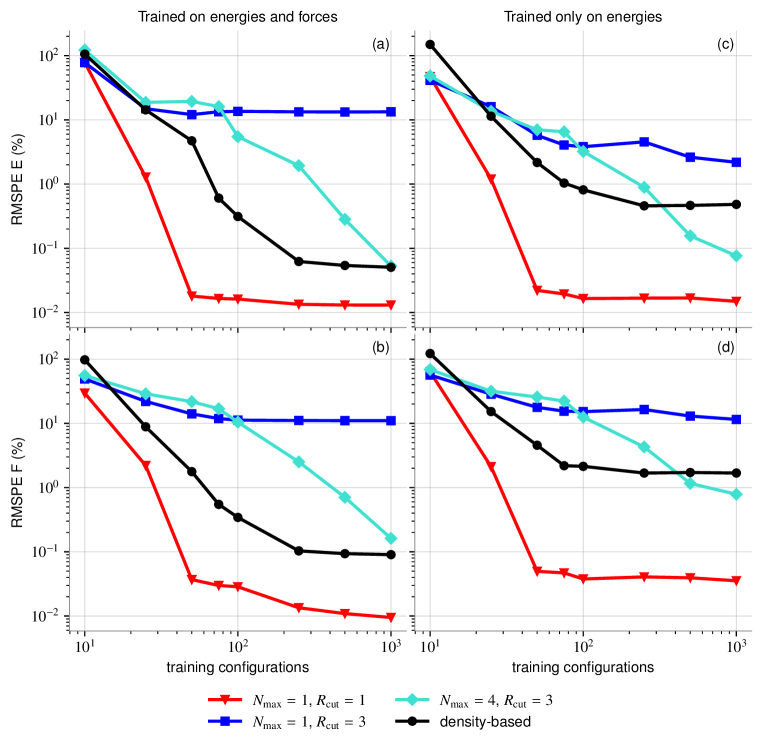
Figure 2: The learning curves for various LODE models using different cutoff-radii $R_{\text{cut}}$ and number of radial basis functions $N_{\text{max}}$ and our density model differ when trained solely on energies. The top panels display the relative percentage error for energy, while the bottom panels present the relative error for the forces. The left panels show the results of training on energies and forces, while the right panels show the results of training on energies only.

The red line represents the ideal LODE descriptor, which quantifies the electrostatic potential inside the sphere of small radius $R_{\text{cut}}$ around the central atom. The electrostatic interaction between two point charges $i$ and $j$ is given by

$$V_{ij}=\frac{1}{2}\frac{Z_{i}Z_{j}}{\|\textbf{r}_{i}-\textbf{r}_{j}\|}$$ (21)

where $\textbf{r}_{i}$ and $\textbf{r}_{j}$ are the positions of the particles and $Z_{i}$ and $Z_{j}$ are their charges. Since the descriptors include information about each atom type $J$ independently the charges are not relevant for the implementation and can be set to one. Then the regression will essentially determine $Z_{i}Z_{j}$.
If one takes now the sum over all pairs $(i,j)$ and over all atoms the electrostatic energy $E$ of the system

$$E=\frac{1}{2}\sum_{i}Z_{i}\sum_{j\neq i}\frac{Z_{j}}{\|\textbf{r}_{i}-\textbf{r}_{j}\|}=\frac{1}{2}\sum_{i}Z_{i}\phi(\textbf{r}_{i})$$ (22)

is obtained as a function of the electrostatic potential $\textbf{r}_{i}$

$$\phi(\textbf{r}_{i})=\sum_{j\neq i}\frac{Z_{j}}{\|\textbf{r}_{i}-\textbf{r}_{j}\|}.$$ (23)

This potential is exactly "measured" by the LODE descriptor with one radial basis function if the cutoff radius is smaller than the minimal atomic distance (the Gaussian broadening adds additional width to the source charges tough). The use of a cutoff sphere is possible due to the Gauss law. According to this, the electrostatic potential at the center of the sphere can be determined by a probe charge of finite size, as long as there is no source term inside the sphere.
With a cutoff radius of 3 Å, the value measured by the single descriptor does not correspond exactly to the value of the potential at the center of the sphere. In this case, the electrostatic potential of point charges that enter the projection sphere can not determined accurately. This is why the blue line levels off at relatively high RMSPEs. Generally, considering the Gaussian broadening $\sigma=0.3$ of the atomic source charges, a cutoff radius of $R_{\text{cut}}\lesssim 2.5~{}$Å$-5\sigma$ must be chosen, where $2.5~{}$Å is the shortest nearest neighbor distance in our models and a factor 5 before $\sigma$ assures that the broadened charge has decayed to negligible values.
When using four radial basis functions (turquoise line), a linear combination of the values of the descriptors can approximate a $\delta$-function at the origin, although the model requires additional training data to learn the precise linear combination that corresponds best to the $\delta$ function.

When training only on energies and predicting forces (as shown in Fig. 2(c) and (d)), the energy predictions are mostly more accurate. However, the errors in the predicted forces are notably higher and seem to stagnate at some point. The same precision as in the mixed training on energies and forces is never reached. This indicates that the models require information about the forces to make highly accurate predictions.

A comparison of our density-based descriptor with the ideal LODE descriptor for this material reveals that the LODE descriptor is superior. While our density-based descriptor yields satisfactory results, it is necessary to employ more radial basis functions (specifically, six instead of one) and perform a hyperparameter search to identify the optimal choice of $\zeta_{\text{max}}$, scaling constant $s$, and the number of radial basis functions. This demonstrates that our density-based descriptor, as predicted by theory, is not the best possible descriptor for this prototypical system. Nevertheless, it is still capable of accurately describing the interactions, albeit requiring more training data.

It is noteworthy that the LODE descriptor with one radial basis function and a cutoff radius smaller than the minimal atomic distance (red line) and the density-based descriptor (black line) can achieve errors below 1% when sufficient training data are used. The LODE descriptor requires only about 40 training structures to achieve a relative error of 1%. The density-based descriptor requires 250 training structures to achieve the same accuracy and then stagnates. We believe the stagnation at very small errors is likely related to the condition number of the design problem becoming very large, which makes it difficult for the pseudo-inversion to separate "noise" from relevant data. Nevertheless, both models give very satisfactory results. These are better than those typically obtained using machine learning, as the errors for MLFFs are typically in the mid-single digit percentage range (around 2 to 10%). The hyperparameters, such as the number of radial basis functions and reciprocal lattice points, can be adjusted to increase the speed and memory efficiency of our computations while still achieving excellent results.

III.2 Sodium Chloride

After demonstrating the models’ ability to describe systems with purely long-range interactions, they were applied to real materials. Liquid sodium chloride (NaCl) was chosen as the first material due to the significant difference in electronegativity between the Na and Cl atoms, which suggests the presence of non-negligible long-range electrostatic interactions. The combined descriptors capture both short- and long-range interactions, enabling analysis of material properties depending on both types of interactions.
The dataset for this material consists of 1014 different structures, each containing 64 Na and 64 Cl atoms. The configurations are taken from VASP molecular dynamics (MD) simulations with 50000 steps and a time step of 1.5 fs. During this run the material was heated from 1100K to 1400K using the Langevin thermostat. An energy cutoff of 350 eV was used. The PAW potentials used were "PAW_PBE Na_pv 19Sep2006" for Na and "PAW_PBE Cl 06Sep2006" for Cl, considering seven valence electrons for each element.

Table 1 presents the results for NaCl obtained using five different methods: purely local/short-range descriptors (Local), MACE without MP (MACE no MP), LODE combined with short-range descriptors (LODE), long-range density-based descriptors combined with short-range descriptors (Density) and MACE with one MP layer (MACE). The combination of short- and long-range descriptors follows the procedure outlined in Eq. (15).
For the short-range part of the descriptor, the hyperparameters were set to $\sigma=0.5$, $R_{\text{cut}}=~{}$6 Å, $N_{\text{max}}=6$ and $L_{\text{max}}=3$ where $L_{\text{max}}$ corresponds to the angular quantum number and indicates the number of angular basis functions. For the density-based part, the optimal choice was $N_{\text{max}}=7$, $s=2$, $\zeta_{\text{max}}=1.5$ and $\sigma=0.3$. For the LODE part $R_{\text{cut}}=$ 1 Å, $N_{\text{max}}=1$ and $\sigma=0.3$ were used. A polynomial kernel of order $\zeta=4$ was used.
For MACE, only invariant features, $R_{\text{cut}}=~{}$6 Å, descriptors with up to four-body interactions, force weights of $1000$, energy weights of $10$ and $100$ epochs were used. After $80$ epochs the energy weights are increased to lower the error in the energies.
Out of the 1014 training configurations always $20\%$ were used as validation data.

Table 1: The root-mean-square percentage error (RMSPE) was calculated for the validation data of liquid NaCl using combined density and LODE descriptors as well as local-only descriptors and MACE Batatia et al. (2022) with and without Message Passing (MP). Radial cutoffs of typically 6 Å are used. The results show that our density-based approach outperforms the LODE method for real materials and is as effective as MACE with MP. Nevertheless, including long-range interactions is essential as the purely local scheme and MACE without MP yield large errors.

	Local	MACE no MP	LODE	Density	MACE
RMSPE E (%)	7.7	8.5	8.1	2.2	3.0
RMSPE F (%)	12.6	8.5	8.7	3.3	3.1

The density-based descriptors and Message Passing MACE outperform the purely local method. LODE performs similarly to MACE with no MP.
When comparing the LODE method and the density-based approach, it is evident that the density-based descriptors perform better. This is because LODE is optimal for purely electrostatic interactions, yet lacks the capability to describe intermediate range interactions. In real materials, the $Z_{i}Z_{j}/\|\textbf{r}_{ij}\|=Z_{i}Z_{j}/r_{ij}$ coulomb interaction between particles $i$ and $j$ is screened by the electrons, resulting in an effective interaction

$$V=\int\frac{Z_{i}Z_{j}}{\left\|\textbf{r}_{i}-\textbf{r}^{\prime}\right\|}\epsilon^{-1}\left(\textbf{r}^{\prime},\textbf{r}_{j}\right)\text{d}^{3}r^{\prime}.$$ (24)

At very large distances the interaction will be screened by the ion-damped macroscopic dielectric constant $\epsilon^{-1}$. However, at medium distance, the electronic screening is less pronounced. LODE is designed to model $1/r$ interactions but not screened interactions $V$. The present approach is far more flexible.

Even when the cutoff radius $R_{\text{cut}}$ of the purely local method is systematically increased to make the descriptors longer-ranged the result never becomes quite as good as for the combined density method or MACE. This is shown in Fig. 3. These data were calculated using the MLFF implemented in VASP. For the three-body descriptors a cutoff radius of $5$ Å was used since this yields better results than 6 Å. This is also the reason why the initial value in this plot is better than the one shown in Tab. 1 obtained using polipy4vasp. In polipy4vasp a distinction between two-body and three-body cutoffs is not possible and the best compromise is found to be 6 Å. The initial error (9.8%) is comparable to MACE without MP (8%) but requires us to perform a hyperparameter search for the cutoff of the three-body terms. As shown in Fig. 3, the error decreases as the cutoff of the two-body descriptors increases, reaching a value slightly below 5 % when the cutoff is sufficiently large. In summary, naively increasing the two-body cutoff does not quite allow us to recover the accuracy of the long-range models. Nevertheless, the present observations have prompted us to routinely use relatively larger cutoffs for the two-body descriptors (8 Å), and fairly small radial cutoffs for the three-body descriptors (5 Å) in VASP.

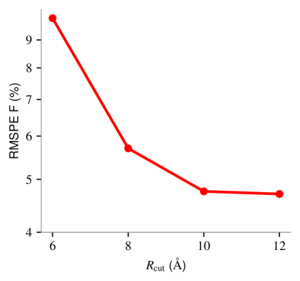
Figure 3: RMSPE in the forces as a function of the two-body cutoff radius $R_{\text{cut}}$ for NaCl for the short-range descriptors. Data was calculated using VASP. Even when the cut-off radius is increased to 12 Å  the local method is unable to match the accuracy of the combined density method or MACE.

As with the hyperparameter optimization demonstrated for the gas of point charges, the hyperparameters for NaCl also required optimization. During this process, we observed that the inclusion of unnecessary information, such as additional long-range radial basis functions with exponents that decay more slowly than necessary for the description of electrostatic interactions in this material, negatively impacts the predictive capability of the model. The addition of radial basis functions that do not encode relevant physical information to the descriptor results in a distortion of the similarity measure of the kernel. Descriptors that have a high degree of similarity with respect to the kernel measure may exhibit a reduction in this similarity when the additional, irrelevant information is added. Thus, the inclusion of irrelevant information reduces the learning efficiency.
Furthermore, the inclusion of irrelevant information in the description worsens the condition number of the design matrix and the numerical stability of the problem.
Particularly when considering long-range descriptors, it is crucial to carefully select the information to be included. Ideally, all hyperparameters that are relevant for the exponents of the exponentially decaying radial basis functions in the density-based approach should be optimized through a grid search for each material separately.

III.3 Zirconia

Bulk zirconia ($\text{ZrO}_{\text{2}}$) is another material with a significant difference in electronegativity between its two atom types. It is used as a second test material for the descriptors developed here. The combined descriptors and the LODE method are used to assess the model’s performance.
The data set of this material consists of 592 distinct structures, each containing 32 Zr and 64 O atoms. The configurations are taken from VASP MD simulations. During these simulations, the material was heated between 300K to 2800K using the Langevin thermostat. For further details on the data set we refer to Ref. Verdi et al. (2021).
Again $20\%$ out of 592 training structures are used for validation.
The hyperparameters used for the short-range parts and MACE were identical to those employed for NaCl. However, for the density-based descriptor, choosing $N_{\text{max}}=5$, $s=1.5$, $\zeta_{\text{max}}=2$ yields the best results. The LODE method, when using $N_{\text{max}}=4$ and $R_{\text{cut}}=3~{}$Å instead of $N_{\text{max}}=1$ and $R_{\text{cut}}=1~{}$Å, yielded slightly better results. Therefore, these values were used in the subsequent calculations.

A comparison of the results for zirconia in Tab. 2 shows that the MACE with MP yields the smallest error. However, the purely local methods result in errors in the single-digit percentage range, indicating that the system is already well-described using only short-range descriptors. The addition of long-range entries from the density-based and LODE method does not significantly alter the results.

Table 2: The root-mean-square percentage error (RMSPE) was calculated for the validation data of ZrO₂ using combined density and LODE descriptors, as well as local-only descriptors and MACE Batatia et al. (2022), with and without Message Passing (MP). For a cutoff radius of $6$ Å in the short-range part of the descriptor, there is hardly any difference between the three kernel methods and they do not reach the accuracy of MACE. However, the error is slightly smaller when long-range electrostatic interactions are included.

	Local	MACE no MP	LODE	Density	MACE
RMSPE E (%)	1.8	1.7	1.9	1.4	1.0
RMSPE F (%)	6.8	6.0	6.3	6.2	3.3

As both the LODE and the density-based model describe only monopole-monopole interactions and yield results that are as good as those of the local description, it can be concluded that no significant monopole-monopole interactions are present in zirconia.
When comparing MACE with and without MP it is evident that the long-range MP model improves the results. We speculate that this implies that, despite the absence of monopole-monopole interactions in zirconia, higher-order long-range electrostatic interactions, such as dipole-dipole interactions, play an important role. Although our results are indirect, we suspect that MACE (as well as other message-passing networks) can describe dynamical long-range dipole-dipole interactions. Considering their architecture, they should be able to learn the dynamic, displacement-induced dipoles on one site (1st MP layer) and their interaction with other sites (2nd MP layer).

IV Conclusion

MLFFs have advanced significantly over the past years, with the equivariant message passing networks in particular greatly improving prediction quality for materials where some form of long-range physics is involved. The consensus seems to be that for solid-state materials, message-passing networks improve the accuracy typically by a factor of two to three compared to more traditional invariant perceptions or standard kernel-based approaches.

The exact reason for this is not yet fully understood. The present work aims to take a rational approach to the problem and attempts to propose long-range descriptors that are capable of describing a specific type of long-range interaction. Our starting point is the long-distance equivariant (LODE) approach, which is designed to describe electrostatic interactions between charges Grisafi and Ceriotti (2019) but also dipoles Grisafi, Nigam, and Ceriotti (2021); Huguenin-Dumittan et al. (2023). The important difference is that we wanted to stick to the standard kind of descriptors that express the environment of an atom in a suitable set of invariant descriptors. It turns out that this is possible and only requires one to abandon the finite-range projectors usually used to describe the environment.

We show that the present long-range descriptor can achieve almost the same accuracy as the LODE descriptors for point charge models. Matter of fact, the learning efficiency is worse than for LODE, since the machine learning model has to determine from the data which linear combination of descriptors describes the Coulomb $1/r$ law. However, the present approach is more flexible as it can, by construction, describe any, e.g. a screened Coulomb, interaction. We demonstrate this for a real material, liquid NaCl, where the interactions are dominated by electrostatic interactions between point charges. However, these interactions are screened by the electrons and the screening is distance-dependent. In this case, the present density-based descriptors combined with the usual short-range descriptors outperform LODE combined with short-range descriptors. Nevertheless, the model is found to be only as accurate as MACE and cannot improve upon the flexible message-passing model.

For the second test material, ZrO₂, we find no improvement using long-range descriptors, and the performance of MACE cannot be matched. This indicates that we are still lacking important physics in the descriptors considered here. The likely explanation is that in ZrO₂ the dynamical (Born effective) charges are strongly anisotropic, i.e. moving in the O-Zr bond direction and orthogonally to them, respectively, gives very different Born effective charges. Our surrogate model is not able to describe this by construction (it rather assumes an isotropic, possibly screened interaction).

Clearly, more work is needed to fully understand what kind of physics needs to be included to improve the short-range models that have dominated research over the last decade. We believe that this rational approach remains relevant, even though data-based flexible message-passing networks are now outperforming the rationally designed surrogate models.

V Acknowledgements

This research was funded in whole by the Austrian Science Fund (FWF) 10.55776/F81. For open access purposes, the author has applied a CC BY public copyright license to any author accepted manuscript version arising from this submission. The presented computational results have been largely obtained using the Vienna Scientific Cluster (VSC).

References

- Grisafi and Ceriotti (2019) A. Grisafi and M. Ceriotti, “Incorporating long-range physics in atomic-scale machine learning,” The Journal of Chemical Physics 151 (2019), 10.1063/1.5128375.
- Manzhos and Carrington (2006) S. Manzhos and T. Carrington, “A random-sampling high dimensional model representation neural network for building potential energy surfaces,” The Journal of chemical physics 125 (2006).
- Behler and Parrinello (2007) J. Behler and M. Parrinello, “Generalized neural-network representation of high-dimensional potential-energy surfaces,” Phys. Rev. Lett. 98, 146401 (2007).
- Bartók et al. (2010) A. P. Bartók, M. C. Payne, R. Kondor, and G. Csányi, “Gaussian approximation potentials: The accuracy of quantum mechanics, without the electrons,” Phys. Rev. Lett. 104, 136403 (2010).
- Rupp et al. (2012) M. Rupp, A. Tkatchenko, K.-R. Müller, and O. A. Von Lilienfeld, “Fast and accurate modeling of molecular atomization energies with machine learning,” Physical review letters 108, 058301 (2012).
- Behler (2015) J. Behler, “Constructing high-dimensional neural network potentials: a tutorial review,” International Journal of Quantum Chemistry 115, 1032–1050 (2015).
- Thompson et al. (2015) A. Thompson, L. Swiler, C. Trott, S. Foiles, and G. Tucker, “Spectral neighbor analysis method for automated generation of quantum-accurate interatomic potentials,” Journal of Computational Physics 285, 316–330 (2015).
- Morawietz et al. (2016) T. Morawietz, A. Singraber, C. Dellago, and J. Behler, “How van der waals interactions determine the unique properties of water,” Proceedings of the National Academy of Sciences 113, 8368–8373 (2016).
- Bartók et al. (2018) A. P. Bartók, J. Kermode, N. Bernstein, and G. Csányi, “Machine learning a general-purpose interatomic potential for silicon,” Physical Review X 8, 041048 (2018).
- Schütt et al. (2018) K. T. Schütt, H. E. Sauceda, P.-J. Kindermans, A. Tkatchenko, and K.-R. Müller, “SchNet – A deep learning architecture for molecules and materials,” The Journal of Chemical Physics 148, 241722 (2018).
- Deringer, Caro, and Csányi (2019) V. L. Deringer, M. A. Caro, and G. Csányi, “Machine learning interatomic potentials as emerging tools for materials science,” Advanced Materials 31, 1902765 (2019).
- Drautz (2019) R. Drautz, “Atomic cluster expansion for accurate and transferable interatomic potentials,” Physical Review B 99, 014104 (2019).
- von Lilienfeld, Müller, and Tkatchenko (2020) O. A. von Lilienfeld, K.-R. Müller, and A. Tkatchenko, “Exploring chemical compound space with quantum-based machine learning,” Nature Reviews Chemistry 4, 347–358 (2020).
- von Lilienfeld and Burke (2020) O. A. von Lilienfeld and K. Burke, “Retrospective on a decade of machine learning for chemical discovery,” Nature Communications 11 (2020).
- Unke et al. (2021a) O. T. Unke, S. Chmiela, H. E. Sauceda, M. Gastegger, I. Poltavsky, K. T. Schütt, A. Tkatchenko, and K.-R. Müller, “Machine learning force fields,” Chemical Reviews 121, 10142–10186 (2021a), pMID: 33705118.
- Keith et al. (2021) J. A. Keith, V. Vassilev-Galindo, B. Cheng, S. Chmiela, M. Gastegger, K.-R. Müller, and A. Tkatchenko, “Combining machine learning and computational chemistry for predictive insights into chemical systems,” Chemical Reviews 121, 9816–9872 (2021).
- Batzner et al. (2022) S. Batzner, A. Musaelian, L. Sun, M. Geiger, J. Mailoa, M. Kornbluth, N. Molinari, T. Smidt, and B. Kozinsky, “E(3)-equivariant graph neural networks for data-efficient and accurate interatomic potentials,” Nature Communications 13 (2022), 10.1038/s41467-022-29939-5.
- Batatia et al. (2022) I. Batatia, D. P. Kovacs, G. Simm, C. Ortner, and G. Csányi, “Mace: Higher order equivariant message passing neural networks for fast and accurate force fields,” (2022).
- Ko and Ong (2023) T. W. Ko and S. P. Ong, “Recent advances and outstanding challenges for machine learning interatomic potentials,” Nature Computational Science 3 (2023).
- Merchant et al. (2023) A. Merchant, S. Batzner, S. Schoenholz, M. Aykol, G. Cheon, and E. Cubuk, “Scaling deep learning for materials discovery,” Nature 624, 1–6 (2023).
- Batatia et al. (2023) I. Batatia, P. Benner, Y. Chiang, A. M. Elena, D. P. Kovács, J. Riebesell, X. R. Advincula, M. Asta, W. J. Baldwin, N. Bernstein, A. Bhowmik, S. M. Blau, V. Cărare, J. P. Darby, S. De, F. D. Pia, V. L. Deringer, R. Elijošius, Z. El-Machachi, E. Fako, A. C. Ferrari, A. Genreith-Schriever, J. George, R. E. A. Goodall, C. P. Grey, S. Han, W. Handley, H. H. Heenen, K. Hermansson, C. Holm, J. Jaafar, S. Hofmann, K. S. Jakob, H. Jung, V. Kapil, A. D. Kaplan, N. Karimitari, N. Kroupa, J. Kullgren, M. C. Kuner, D. Kuryla, G. Liepuoniute, J. T. Margraf, I.-B. Magdău, A. Michaelides, J. H. Moore, A. A. Naik, S. P. Niblett, S. W. Norwood, N. O’Neill, C. Ortner, K. A. Persson, K. Reuter, A. S. Rosen, L. L. Schaaf, C. Schran, E. Sivonxay, T. K. Stenczel, V. Svahn, C. Sutton, C. van der Oord, E. Varga-Umbrich, T. Vegge, M. Vondrák, Y. Wang, W. C. Witt, F. Zills, and G. Csányi, “A foundation model for atomistic materials chemistry,” (2023), arXiv:2401.00096 [physics.chem-ph] .
- Kjellander (2018) R. Kjellander, “Focus Article: Oscillatory and long-range monotonic exponential decays of electrostatic interactions in ionic liquids and other electrolytes: The significance of dielectric permittivity and renormalized charges,” The Journal of Chemical Physics 148, 193701 (2018).
- Guo et al. (2018) Z. Guo, F. Ambrosio, W. Chen, P. Gono, and A. Pasquarello, “Alignment of redox levels at semiconductor–water interfaces,” Chemistry of Materials 30, 94–111 (2018).
- Jorn et al. (2013) R. Jorn, R. Kumar, D. P. Abraham, and G. A. Voth, “Atomistic modeling of the electrode–electrolyte interface in li-ion energy storage systems: Electrolyte structuring,” The Journal of Physical Chemistry C 117, 3747–3761 (2013).
- French et al. (2010) R. H. French, V. A. Parsegian, R. Podgornik, R. F. Rajter, A. Jagota, J. Luo, D. Asthagiri, M. K. Chaudhury, Y.-m. Chiang, S. Granick, S. Kalinin, M. Kardar, R. Kjellander, D. C. Langreth, J. Lewis, S. Lustig, D. Wesolowski, J. S. Wettlaufer, W.-Y. Ching, M. Finnis, F. Houlihan, O. A. von Lilienfeld, C. J. van Oss, and T. Zemb, “Long range interactions in nanoscale science,” Rev. Mod. Phys. 82, 1887–1944 (2010).
- Ko et al. (2021) T. W. Ko, J. A. Finkler, S. Goedecker, and J. Behler, “A fourth-generation high-dimensional neural network potential with accurate electrostatics including non-local charge transfer,” Nature Communications 12 (2021), 10.1038/s41467-020-20427-2.
- Unke et al. (2021b) O. T. Unke, S. Chmiela, M. Gastegger, K. T. Schütt, H. E. Sauceda, and K.-R. Müller, “SpookyNet: Learning force fields with electronic degrees of freedom and nonlocal effects,” Nature Communications 12 (2021b), 10.1038/s41467-021-27504-0.
- Ambrosetti et al. (2016) A. Ambrosetti, N. Ferri, R. A. DiStasio, and A. Tkatchenko, “Wavelike charge density fluctuations and van der waals interactions at the nanoscale,” Science 351, 1171–1176 (2016).
- Stöhr and Tkatchenko (2019) M. Stöhr and A. Tkatchenko, “Quantum mechanics of proteins in explicit water: The role of plasmon-like solute-solvent interactions,” Science Advances 5, eaax0024 (2019).
- Unke et al. (2022) O. T. Unke, M. Stöhr, S. Ganscha, T. Unterthiner, H. Maennel, S. Kashubin, D. Ahlin, M. Gastegger, L. M. Sandonas, A. Tkatchenko, and K.-R. Müller, “Accurate machine learned quantum-mechanical force fields for biomolecular simulations,” (2022), arXiv:2205.08306 [physics.chem-ph] .
- Grisafi, Nigam, and Ceriotti (2021) A. Grisafi, J. Nigam, and M. Ceriotti, “Multi-scale approach for the prediction of atomic scale properties,” Chem. Sci. 12, 2078–2090 (2021).
- Zhang et al. (2022) L. Zhang, H. Wang, M. C. Muniz, A. Z. Panagiotopoulos, R. Car, and W. E, “A deep potential model with long-range electrostatic interactions,” The Journal of Chemical Physics 156 (2022), 10.1063/5.0083669.
- Bereau et al. (2018) T. Bereau, J. DiStasio, Robert A., A. Tkatchenko, and O. A. von Lilienfeld, “Non-covalent interactions across organic and biological subsets of chemical space: Physics-based potentials parametrized from machine learning,” The Journal of Chemical Physics 148, 241706 (2018).
- Yao et al. (2018) K. Yao, J. E. Herr, D. W. Toth, R. Mckintyre, and J. Parkhill, “The tensormol-0.1 model chemistry: a neural network augmented with long-range physics,” Chem. Sci. 9, 2261–2269 (2018).
- Unke and Meuwly (2019) O. T. Unke and M. Meuwly, “Physnet: A neural network for predicting energies, forces, dipole moments, and partial charges,” Journal of Chemical Theory and Computation 15, 3678–3693 (2019).
- Niblett, Galib, and Limmer (2021) S. P. Niblett, M. Galib, and D. T. Limmer, “Learning intermolecular forces at liquid–vapor interfaces,” The Journal of Chemical Physics 155, 164101 (2021).
- Gao and Remsing (2022) A. Gao and R. C. Remsing, “Self-consistent determination of long-range electrostatics in neural network potentials,” Nature communications 13, 1572 (2022).
- Huguenin-Dumittan et al. (2023) K. K. Huguenin-Dumittan, P. Loche, N. Haoran, and M. Ceriotti, “Physics-inspired equivariant descriptors of nonbonded interactions,” The Journal of Physical Chemistry Letters 14, 9612–9618 (2023).
- Bishop (2010) C. M. Bishop, Pattern recognition and machine learning, corr. at 8th print. ed., Information science and statistics (Springer, New York, NY, 2010).
- Gilmer et al. (2017) J. Gilmer, S. S. Schoenholz, P. F. Riley, O. Vinyals, and G. E. Dahl, “Neural message passing for quantum chemistry,” in Proceedings of the 34th International Conference on Machine Learning, Proceedings of Machine Learning Research, Vol. 70, edited by D. Precup and Y. W. Teh (PMLR, 2017) pp. 1263–1272.
- Bronstein et al. (2021) M. M. Bronstein, J. Bruna, T. Cohen, and P. Veličković, “Geometric deep learning: Grids, groups, graphs, geodesics, and gauges,” (2021), arXiv:2104.13478 [cs.LG] .
- Haghighatlari et al. (2022) M. Haghighatlari, J. Li, X. Guan, O. Zhang, A. Das, C. J. Stein, F. Heidar-Zadeh, M. Liu, M. Head-Gordon, L. Bertels, et al., “Newtonnet: A newtonian message passing network for deep learning of interatomic potentials and forces,” Digital Discovery 1, 333–343 (2022).
- Gasteiger, Groß, and Günnemann (2022) J. Gasteiger, J. Groß, and S. Günnemann, “Directional message passing for molecular graphs,” (2022), arXiv:2003.03123 [cs.LG] .
- Takamoto, Izumi, and Li (2022) S. Takamoto, S. Izumi, and J. Li, “Teanet: Universal neural network interatomic potential inspired by iterative electronic relaxations,” Computational Materials Science 207, 111280 (2022).
- Chen and Ong (2022) C. Chen and S. P. Ong, “A universal graph deep learning interatomic potential for the periodic table,” Nature Computational Science 2, 718–728 (2022).
- Deng et al. (2023) B. Deng, P. Zhong, K. Jun, J. Riebesell, K. Han, C. J. Bartel, and G. Ceder, “Chgnet as a pretrained universal neural network potential for charge-informed atomistic modelling,” Nature Machine Intelligence 5, 1031–1041 (2023).
- Jinnouchi, Karsai, and Kresse (2019) R. Jinnouchi, F. Karsai, and G. Kresse, “On-the-fly machine learning force field generation: Application to melting points,” Phys. Rev. B 100, 014105 (2019).
- Jinnouchi et al. (2019) R. Jinnouchi, J. Lahnsteiner, F. Karsai, G. Kresse, and M. Bokdam, “Phase transitions of hybrid perovskites simulated by machine-learning force fields trained on the fly with bayesian inference,” Phys. Rev. Lett. 122, 225701 (2019).
- Jinnouchi et al. (2020a) R. Jinnouchi, F. Karsai, C. Verdi, R. Asahi, and G. Kresse, “Descriptors representing two- and three-body atomic distributions and their effects on the accuracy of machine-learned inter-atomic potentials,” The Journal of Chemical Physics 152, 234102 (2020a).
- Jinnouchi et al. (2020b) R. Jinnouchi, K. Miwa, F. Karsai, G. Kresse, and R. Asahi, “On-the-fly active learning of interatomic potentials for large-scale atomistic simulations,” The Journal of Physical Chemistry Letters 11, 6946–6955 (2020b).
- Bartók, Kondor, and Csányi (2013) A. P. Bartók, R. Kondor, and G. Csányi, “On representing chemical environments,” Phys. Rev. B 87, 184115 (2013).
- Häser and Almlöf (1992) M. Häser and J. Almlöf, “Laplace transform techniques in Mo/ller–Plesset perturbation theory,” The Journal of Chemical Physics 96, 489–494 (1992), https://pubs.aip.org/aip/jcp/article-pdf/96/1/489/18996860/489_1_online.pdf .
- Izmaylov and Scuseria (2008) A. F. Izmaylov and G. E. Scuseria, “Resolution of the identity atomic orbital laplace transformed second order møller–plesset theory for nonconducting periodic systems,” Phys. Chem. Chem. Phys. 10, 3421–3429 (2008).
- Doser, Lambrecht, and Ochsenfeld (2008) B. Doser, D. S. Lambrecht, and C. Ochsenfeld, “Tighter multipole-based integral estimates and parallel implementation of linear-scaling ao–mp2 theory,” Phys. Chem. Chem. Phys. 10, 3335–3344 (2008).
- Ayala and Scuseria (1999) P. Y. Ayala and G. E. Scuseria, “Linear scaling second-order Moller–Plesset theory in the atomic orbital basis for large molecular systems,” The Journal of Chemical Physics 110, 3660–3671 (1999), https://pubs.aip.org/aip/jcp/article-pdf/110/8/3660/19255870/3660_1_online.pdf .
- Kaltak, Klimes, and Kresse (2014) M. Kaltak, J. Klimes, and G. Kresse, “Low scaling algorithms for the random phase approximation: Imaginary time and laplace transformations,” Journal of chemical theory and computation 10, 2498–2507 (2014).
- Schmiedmayer and Kresse (2024) B. Schmiedmayer and G. Kresse, “Derivative learning of tensorial quantities – predicting finite temperature infrared spectra from first principles,” (2024), arXiv:2404.19674 .
- Kresse and Furthmüller (1996a) G. Kresse and J. Furthmüller, “Efficiency of ab-initio total energy calculations for metals and semiconductors using a plane-wave basis set,” Computational materials science 6, 15–50 (1996a).
- Kresse and Furthmüller (1996b) G. Kresse and J. Furthmüller, “Efficient iterative schemes for ab initio total-energy calculations using a plane-wave basis set,” Physical review B 54, 11169 (1996b).
- Kresse and Joubert (1999) G. Kresse and D. Joubert, “From ultrasoft pseudopotentials to the projector augmented-wave method,” Physical review b 59, 1758 (1999).
- Verdi et al. (2021) C. Verdi, F. Karsai, P. Liu, R. Jinnouchi, and G. Kresse, “Thermal transport and phase transitions of zirconia by on-the-fly machine-learned interatomic potentials,” npj Computational Materials 7 (2021), 10.1038/s41524-021-00630-5.