Learning Dynamic Bayesian Networks from Data: Foundations, First Principles and Numerical Comparisons

Abstract

In this paper, we present a guide to the foundations of learning Dynamic Bayesian Networks (DBNs) from data in the form of multiple samples of trajectories for some length of time. We present the formalism for a generic as well as a set of common types of DBNs for particular variable distributions. We present the analytical form of the models, with a comprehensive discussion on the interdependence between structure and weights in a DBN model and their implications for learning. Next, we give a broad overview of learning methods and describe and categorize them based on the most important statistical features, and how they treat the interplay between learning structure and weights. We give the analytical form of the likelihood and Bayesian score functions, emphasizing the distinction from the static case. We discuss functions used in optimization to enforce structural requirements. We briefly discuss more complex extensions and representations. Finally we present a set of comparisons in different settings for various distinct but representative algorithms across the variants.

1 Introduction

In this paper we give a comprehensive presentation on the training of Dynamic Bayesian Networks (DBNs), including both structure and parameters, from data. DBNs present a naturally interpretable model when it comes to understanding the precise interaction underlying the relationship between the variables. That is, the conditional independence structure defined by the DBN provides information regarding the mechanistic procedure that defines the model. This is also associated with the field of statistics referred to as causal learning.

There is one general survey article on DBNs we found is [59], which provides a helpful comprehensive resource for references for DBN modeling, inference and learning. In this work rather than seeking to provide a comprehensive literature review, instead we focus on narrating the global landscape of the mathematical understanding of the most important considerations as far as learning a model, including both the structure and parameters, from data.

With this understanding we are able to establish an informative taxonomy regarding methods, providing transparency in regards to the function and intention of each method. There are important subtle distinctions as far as modeling assumptions between some different popular methods, and their awareness is critical for best practices of DBN learning. Finally, we perform comprehensive numerical comparisons, highlighting the particular advantages and disadvantages of each method. We highlight that these comparisons are not meant to be exhaustive or authoritative, but more informative and illustrative in regards to the tradeoffs associated with learning DBNs from data.

We make several assumptions for this work. These are not entirely formal for the sake of precise Theorem proving, but rather a general restriction of the data generating process of interest, so as to highlight the most pedagogical features of DBN learning, as far as it is most commonly done in the literature. These assumptions are restrictive as far as faithful statistical modeling of real world phenomena. However, they tremendously simplify the learning process, and thus allow a more comprehensible presentation of what can hope to achieve with standard simple methods. For transparency, we present them below.

1. Causal Sufficiency There are no unobserved confounders, i.e., there is a closed system defining the data generating process wherein all causal sources are observed. This permits for the conditional independence structures to be reliable indicators of edge links in the graph. This is a standard formal assumption in almost all learning algorithms for DBNs and BNs.

2. Causal Identifiability we focus on the general case wherein the data regime permits for potential identification of a true causal graph, generally corresponding to the number of data samples (trajectories $\times$ time steps) some exponential factor of mangitude greater than the number of variables (in practice this can mean $5$ variables, $100$ trajectories of each $50$ time steps as a generic example). This permits us to focus on integer programming and other techniques that can obtain statistically significant point estimates for exact structures that recover a ground truth. This assumption is standard in the literature of DBN and SEM learning, as modeling uncertainty in less favorable data regime circumstances presents significant methodological challenges and considerations that require significantly more advanced techniques. However, understanding the nuances of the foundations are essential as far the proper development, implementation, and use of these techniques.

3. Fully Observed There are no hidden variables, all quantities of interest are fully observed at every time step. Of course, graphs with hidden (latent) variables and entire structures are instrumental for modeling in many fields. However, the inclusion of latent variables and the required Expectation Maximization modification of the procedures described presents technical complications that add significant additional complexity, and thus would necessity a much greater length while obfuscating the message.

We make a few departures from these assumptions throughout the work, which we explicitly indicate when they occur.

1.1 Contribution of this Work

In this work we present:

1. A thorough explicit analytical description of standard popular DBN representations and statistical models. This includes the structure of potential dependencies of transition functions of the time-dependent random variables on other variables, time independent as well as time-dependent and in-time, Markovian one time step back, and delayed dependence.

2. Extensive commentary and analysis of learning DBNs from data from both the classical PGM/BN perspective as well as the time series perspective. The relationship of learning to the structure of the data, as well as high level intuition on the complex interaction of learning the structure and the parameters is presented.

3. A presentation of the most standard and common criteria for defining the objective or cost of a particular DBN network structure as well as the functional forms of equations that define that the graph satisfies the structural requirements of a DBN, in particular acyclicity

4. Numerical results for examples of popular algorithms for learning DBNs, evaluated on a range of criteria and variety of problems. The set of examples is not meant to be exhaustive, nor the comparisons authoritative, but broadly illustrative of the relative advantages and disadvantages of the different methods available.

1.2 Applications of Dynamic Bayesian Networks

The discovery of dynamic Bayesian networks has found many applications, some of which are medicine [12, 20, 75, 8], economics [43, 44] and aviation [46, 65, 27]. The applications related to aviation are typically related to finding casual structure in a sub-problem related to the dispatch of flights and focused on risk mitigation. The medial applications typically focus on either the discovery of fundamental principles related to chemical reactions, which take place in biological organisms or the extraction of information from clinical data. In economics, it is typically of interest to uncover relationships between the stock market and other selected factors that either influence or are influenced by it. In the following, we give some details about chosen applications as well as specific outcomes that the modelling using DBNs has in practice.

1.2.1 Medical Science

To highlight the importance of DBN discovery in medicine, we detail three separate applications. The first of these focuses on the quantification of disease development [8]. Understanding the progression of diseases is crucial in clinical medicine, as it informs the effectiveness of treatments. Most clinical medicine and pathology textbooks provide detailed descriptions of disease progression and treatment responses. However, there has been limited research quantifying these descriptions in detail. Typically, research examines the temporal aspect by describing treatment outcomes after a certain period. A significant challenge in gaining deeper insights is the relatively small size of clinical datasets, often comprising only a few hundred patients.

In the aforementioned contribution, a heuristic procedure is proposed for exploring and learning non-homogeneous time dynamic Bayesian networks, aiming to balance specificity and simplicity. The approach begins with a fully homogeneous (in time) model parts of which are gradually replaced with sub-models which reflect the expected structure at a given level of time delay. Furthermore, a splitting technique is applied to further improve the predictive behavior of the model, such models are typically termed partitioned DBNs.

A heuristic method was proposed to learn the DBN on synthetic data, which has a structure that should reflect a real data set. The numerical performance in terms of accuracy and solution time reported is hopeful. However, the method has yet to be tested on real world datasets.

The second application is concerned with the mapping of neural pathways [20]. Identifying functional connectivity from simultaneously recorded spike trains is crucial for understanding how the brain processes information and instructs the body to perform complex tasks. The study investigates the applicability of dynamic Bayesian networks (DBNs) to infer the structure of neural circuits from observed spike trains. A probabilistic point process model was employed to assess performance. The results confirm the utility of DBNs in inferring functional connectivity as well as the directions of signal flow in cortical network models. Additionally, the findings demonstrate that DBNs outperform Granger causality when applied to populations with highly non-linear synaptic integration mechanisms.

The third chosen application focuses on the choice of appropriate treatment regimens for Chronic lymphocytic leukemia (CLL) [75]. This cancer is the most common blood cancer in adults, with a varied course and response to treatment among patients. This variability complicates the selection of the most appropriate treatment regimen and the prediction of disease progression. The aforementioned paper aims to develop and validate dynamic Bayesian networks (DBNs) to predict changes in the health status of patients with CLL and predict the progression of the disease over time. Two DBNs, the Health Status Network (HSN) and the Treatment Effect Network (TEN), were developed and implemented. Relationships linking the most important factors influencing health status and treatment effects in CLL patients were identified based on literature data and expert knowledge. The developed networks, particularly TEN, were able to predict the probability of survival in CLL patients, aligning with survival data collected in large medical registries. The networks can tailor predictions by integrating prior knowledge specific to an individual CLL patient. The proposed approach is a suitable foundation for developing artificial intelligence systems that assist in selecting treatments, thereby positively influencing the chances of survival for CLL patients.

1.2.2 Economics

The relationship between the stock market and national economies deepens as the market matures, highlighting the need to study their dynamic interplay. Economic indicators such as real income and savings rates play crucial roles in influencing stock market capitalization. Macroeconomic fundamentals wield considerable influence over both short and long-term periods. Some researchers argue that finance and economic growth are causally linked, suggesting the stock market’s potential to drive economic development. However, not all macroeconomic factors significantly impact stock prices. Understanding the strength of association among these variables offers insights into how the stock market behaves across varying economic landscapes. Research on the Chinese stock market examines how macroeconomic variables shape stock market indices over time, emphasizing the enduring influence of economic fundamentals amid short-term market fluctuations. The aforementioned interplay may be modeled by DBNs and has been detailed in [44].

In the article and analysis of the relationship between the stock market and economic fundamentals using 11 selected factors is modeled using a DBN. Among these, four factors pertain to stock market indicators, while the remaining factors focus on macroeconomic and policy considerations. The first four factors reflect stock market performance, with defensive and cyclical stocks exhibiting varying behaviors during bull and bear markets. The Stock Exchange 50 index, comprising the 50 largest and most liquid stocks in the Shanghai Securities Market, supplements the overall stock market observation. Additionally, the consumer stock index serves as an indicator of societal consumption levels, typically rising during favorable macroeconomic periods and declining during economic downturns.

The results on real data of the described method are mixed. The application to the Shanghai composite market yielded some positive results in terms of the prediction of macroscopic quantities, but only limited success in terms of constituent market price prediction. The modeling of the components of the market in sufficient detail is a difficult problem due to the numerical tractability being limited as the number of variables increases.

1.2.3 Aviation

The global collection of aircraft and the airspace in which they operate, is a complex system generating a vast amount of data, making it a challenging domain to model mathematically. This system includes critical elements such as aircraft, airports, flight crews, weather events, and routes, each with many subcomponents. For example, aircraft have numerous subsystems and components, each subjected to various stresses and maintenance actions, which influence their time dynamics. Airports have multiple runways and internal logistical processes, which influence the operational capacity. These system components interact in complex ways. For instance, each flight corresponds to an aircraft operated by a flight crew traveling from one airport to another via a route that may need to change due to weather. Multiple flights operate simultaneously, requiring coordination to avoid incidents while maximizing throughput and minimizing delays.

To give an idea about a specific aviation problem that may be tackled we describe the airport operation uncertainty characterisation, which has been developed in [27]. The model outlines aircraft flow through the airport, emphasizing integrated airspace and airside operations. It characterizes various operational milestones based on an aircraft flow’s Business Process Model and Airport Collaborative Decision-Making methodology. Probability distributions for factors influencing aircraft processes need to be estimated, along with their conditional probability relationships. This approach results in a dynamic Bayesian network that manages uncertainties in aircraft operating times at the airport. The nodes of the network describe various aspects of the airport and flight operations. They cover meteorological conditions, arrival airspace variables such as timestamps and congestion metrics, airport infrastructure, operator and flight data, airside operational times and flight regulations, and the causes of delays.

The key outcomes of this work include the statistical characterization of processes and uncertainty drivers, and a causal model for uncertainty management using a DBN. Analyzing 34,000 aircraft operations at Madrid Airport revealed that arrival delays accumulate throughout the day due to network effects, while departure delays do not follow this pattern. The major delay drivers identified were the time of day, ASMA congestion, weather conditions, arrival delay amount, process duration, runway configuration, airline business model, handling agent, aircraft type, route origin/destination, and ATFCM regulations. Departure delays are significantly impacted by events of longer duration, which also offer greater potential for recovery.

2 Background - Dynamic Bayesian Networks

We present the general, and then specific forms, of DBN models. Consider that there is an $n$-dimensional stochastic process $X(t)$. The individual random variables $X_{i}(t)$ for all $i\in[n_{x}]$ can be valued as discrete, or as members of some field, such as $\mathbb{R}$. In addition, there can be an $n_{z}$-dimensional random variable $Z$. Let us denote the generic spaces as $\mathcal{X}$ and $\mathcal{Z}$, respectively.

The defining character of DBNs is modeling the dependence of $X_{i}(t)$ on other quantities, i.e., defining the the evolution of the stochastic process $X(t)\to X(t+1)$. Formally, for the probability kernel defining the iterations of the stochastic process, the dependence must be Markovian, that is

$$p(X_{i}(t+1)\in A)=f_{i}(X(t),X_{j\neq i}(t+1),\{X_{i}(t-\tau)\}_{\tau=1,...,p},Z)$$ (1)

where $A$ is some set in the Borel $\sigma$-algebra of $\mathcal{X}$. That is, the transition kernel can depend on the current state of the other random variables, the values of the random variables at the previous time, the time-independent variables $Z$, as well as a possibly autoregressive effect through dependence on $\{X_{i}(t-\tau)\}_{\tau=1,...,p}$.

In addition, there is the important requirement that no in-time string of dependencies forms a cycle. This presents the necessity in introducing graph theoretical notions to precisely characterize DBNs. Generically, we say a directed graph is a set of vertices $\mathcal{V}=\{v_{1},v_{2},...,v_{n}\}$ and edges $\mathcal{E}=\{e_{1},e_{2},...,e_{m}\}$, where $e_{j}=(v_{j_{1}},v_{j_{2}})$ denotes the existence of a directed path between the two notes $v_{j_{2}}\to v_{j_{1}}$. We also say in this case that $j_{2}$ is a parent of $j_{1}$, or $j_{2}\in dpa(j_{1})$.

The DBN model incorporates a directed acyclic graph (DAG) $\bar{\mathcal{G}}=\mathcal{G}(\mathcal{V}(X(t-1),X(t)),\mathcal{E}_{d})\cup\mathcal{G}(\mathcal{V}(X(t),Z),\mathcal{E}_{z})\cup\mathcal{G}(\mathcal{V}(X(t),X(t-\tau)),\mathcal{E}_{\tau})$. The first two define connections in the model between the temporal random variables. That is $e=\{V_{1},V_{2}\}\in\mathcal{E}_{d}$ with $V_{i}\in\{\{X_{i}\}\}$ if $p(X(t+1)_{i}\in A)$ is a function of $V_{2}=X_{j}$, that is $j\in dpa_{d}(i)$, and $e=\{V_{1},V_{2}\}\in\mathcal{E}_{s}$ if $p(X_{i}(t+1)\in A)$ is a function of $V_{2}=X_{j}(t+1)$, that is $2\in dpa_{s}(i)$. Finally, we also have a (non-symmetric) matrix encoding the dependencies on the self-history $\tau\in dpa_{\tau}(i)\subset\{1,...,p\}$ and the dependencies on the static variables $dpa_{z}(i)=\left\{Z_{j}:\frac{\partial f_{i}(\cdot)}{\partial Z_{j}}\neq 0\right\}$. These, of course, can be encoded as graphs as well.

This permits us to write (1) as,

$$p(X_{i}(t+1)\in A)=f(A,\{X_{j}(t)\}_{j\in dpa_{d}(i)},\{X_{j}(t+1)\}_{j\in dpa_{s}(i)},\{X_{i}(t-\tau)\}_{\tau\in dpa_{\tau}(i)},\{Z_{j}\}_{j\in dpa_{z}(i)})$$ (2)

Notice that the encoding of the explicit dependencies presents the possibility of using a common $f$ as opposed to one depending on the transition out-node $i$, in the case wherein all the variables $X_{i}$ are of the same distributional family. This eases the computation of the likelihood of the data given the parameters and structure, etc.

We will sometimes use, for shorthand:

$$\{V_{j}(t+1)\}_{j\in dpa(i)}=\{X_{j}(t)\}_{j\in dpa_{d}(i)}\cup\{X_{j}(t+1)\}_{j\in dpa_{s}(i)}\cup\{X_{i}(t-\tau)\}_{\tau\in dpa_{\tau}(i)}\cup\{Z_{j}\}_{j\in dpa_{z}(i)}$$ (3)

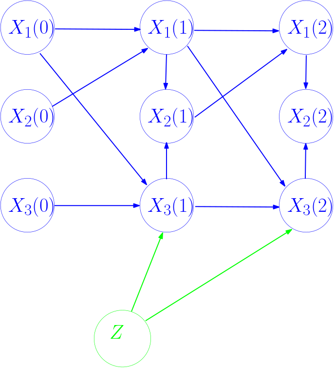
Figure 1: A Possibl DBN Graphical Network defining the transitions of $X(t)$

See Figure 1 for an illustration. In this case for $i=1$, the Markovian transitions are from itself and from $X_{2}$, and there are no intra time nodes or static nodes directed to it, and so $V_{dpa(1)}(t)=V_{dpa_{d}(1)}=\{X_{1}(t-1),X_{2}(t-1)\}$. For node 2, there are no Markovian transitions and two intra-node dependencies, thus $V_{dpa(2)}(t)=V_{dpa_{s}(2)}(t)=\{X_{1}(t),X_{3}(t)\}$. Finally, for $X_{3}(t)$, there are two Markovian dependencies, and a static covariate dependence. Thus $V_{dpa(3)}(t)=V_{dpa_{d}(3)\cup dpa_{z}(3)}(t)=\{X_{1}(t-1),X_{3}(t-1),Z\}$.

Now that we have established the general form of the DBN, we see that we have a fundamentally still very general problem to solve, in that the function $f$ can encode any sort of dependency on the different variables in the parent set of the note of interest. They can depend as according to various nonlinear interactions, that can themselves embody different conditional independence information In order to complete the model, we need to define the form of the function $f$.

2.1 Simple Parametric Conditional Probability Dependency

For certain kinds of variables, it becomes both possible and prudent to use certain simple parametric families for defining $f$. In particular, for binary Bernoulli random variables correspond to Dirichlet distributions for the prior of the weights together with using Conditional Probability Tables to define the form. For continuous random variables, Gaussian linear models provide a means of computing the maximum likelihood linear parameters using covariance matrices.

A significant advantage of using parametric families arises from the closed form computation of criteria, which permits closed form computation of the marginal posterior of a structure. This permits structure learning algorithms to be able to score graphs offline, assisting in the search. Many score maximizing procedures such as [26, 14, 3, 2] use this approach. The score is ultimately an integration of the posterior of the parameters in the model given the structure, which also indicates that the sampling of the optimal parameters, once obtaining the maximum a posteriori structure, is straightforward for these models.

In addition, one can use neural models including the Generative Flow Network approaches as given by [17, 2]. These use a Reinforcement Learning iteration to ultimately sample from a high scoring network as according to a defined score. Reinforcement Learning broadly, e.g., [74] is another framework by which the structure search for these standard specific models can be aided by neural networks.

Linear Structural Equation Models (SEMs) present an opportunity to use an adjacency matrix to define both the structure and weights in a computationally advantageous form. This highlights the correspondence between the Dynamic Systems and the graph theoretic developments in causal learning.

2.1.1 Discrete Variables

Binary Variables

The case of binary random variables is wherein $X_{i}(t)\in B(1,p^{X}_{i}),Z_{j}\sim B(1,p^{Z}_{j})$, etc., that is, they are all of Bernoulli type. Empirical samples for all $k\in[K]$, where $k$ indexes a set of sample trajectories satisfy $X^{(k)}_{i}(t),Z^{(k)}_{j}\in\{0,1\}$ for all $t$, $i$, and $j$. With this most simple scenario, the modeling flexibility as well as the nuances of structure learning becomes a natural pedagogical start.

There is a degree of flexibility in the choice of statistical model for defining the transition function. We will explore three options - the noisy or model, the linear logit model, and the complete linear logit model.

The noisy or model defines the transitions as

$$\begin{array}[]{l}p(X_{i}(t+1)=0)=(1-\lambda_{0})\prod_{l\in dpa(i)}(1-\lambda_{l})^{V_{l}}\\ p(X_{i}(t+1)=1)=1-(1-\lambda_{0})\prod_{l\in dpa(i)}(1-\lambda_{l})^{V_{l}}\end{array}$$ (4)

This model is referred to as noisy or because essentially it calculates a probabilistic perturbation of the binary OR operation. This model presents one implementation of causal independence, wherein the influence of each covariate is independent with respect to the others.

For the linear logit models, define the sigmoid function,

$$\sigma(x)=\frac{e^{x}}{1+e^{x}}$$

The reason the models we define next are referred to as linear is that the transition is defined to be,

$$X_{i}(t+1)=\sum\limits_{j\in dpa_{d}(i)}\beta^{d}_{j}X_{j}(t)+\sum\limits_{j\in dpa_{s}(i)}\beta^{s}_{j}X_{j}(t+1)+\sum\limits_{\tau\in dpa_{\tau}(i)}\beta^{a}_{\tau}X_{i}(t-\tau)+\sum\limits_{j\in dpa_{z}(i)}\beta^{z}_{j}Z_{j}$$ (5)

We shall see that this linear form is broadly common in modeling the transitions of variables in DBN models for other variable types.

The probability kernel given by (5) is

$$p(X_{i}(t+1)=1)=\sigma\left(\beta_{0}+\sum\limits_{j\in dpa_{d}(i)}\beta^{d}_{j}X_{j}(t)+\sum\limits_{j\in dpa_{s}(i)}\beta^{s}_{j}X(t+1)_{j}+\sum\limits_{\tau\in dpa_{\tau}(i)}\beta^{a}_{\tau}X_{i}(t-\tau)+\sum\limits_{j\in dpa_{z}(i)}\beta^{z}_{j}Z_{j}\right)$$ (6)

One alternative that frequently arises in practice is the necessity to accurately model Conditional Probability Dependencies (CPDs) as defined by Conditional Probability Tables (CPTs). As an example, please see Table 1.

Table 1: An example of a CPT

$X_{2}(t)$	$X_{3}(t+1)$	$Z_{2}$	$X_{1}(t+1)$
0	0	0	0
0	0	1	1
0	1	0	1
0	1	1	0
1	0	0	1
1	0	1	0
1	1	0	0
1	1	1	1

It is clear that the information in Table 1 cannot be modeled with a linear transition function as in (5). In this case, if one wanted to construct such a model, one would instead have to be able to include all of the combinations between the possible parent nodes.

Formally, a transition model could look like, for Table 1,

$$\begin{array}[]{l}X_{1}(t+1)=\beta_{0}+\beta_{1}Z_{2}+\beta_{2}X_{3}(t+1)+\beta_{3}X_{3}(t+1)Z_{2}+\beta_{4}X_{3}(t+1)Z_{2}+\beta_{5}X_{2}(t)\\ \qquad\qquad\qquad+\beta_{6}X_{2}(t)Z_{2}+\beta_{7}X_{2}(t)X_{3}(t+1)+\beta_{8}X_{2}(t)X_{3}(t+1)Z_{2}\end{array}$$

and in the general case,

$$\begin{array}[]{l}X_{i}(t+1)=\prod\limits_{j\in dpa_{d}(i)}\prod\limits_{k\in dpa_{s}(i)}\prod\limits_{\tau=1,...,p}\prod\limits_{l\in dpa_{z}(i)}\sum_{\alpha\in\left(\mathbb{Z}^{+}_{2}\right)^{4}}\beta_{i,j,k,l,\tau}^{\alpha}\left(X_{j}(t)X_{k}(t+1)X_{i}(t-\tau)Z_{j}\right)^{\alpha}\end{array}$$ (7)

where the parameters are appropriately normalized. With the combinatorial explosion in this model clearly visible, it can be seen that such circumstances present significant difficulties as far as computing hardware expense in both processing and memory, when it comes to modeling high dimensional datasets.

On the other hand, this structure of statistical model presents two structural conditions denoted as local parameter independence and unrestricted multinomial distribution [61]. These ensure that for every configuration, that is, every possible combinations of values of the parents of a node, there is an independent parameter vector. This leads to a corresponding combinatorial explosion of parameter vectors in the statistical model. On the other hand, however, the analytical calculation of parameter likelihoods and posterior distributions become possible, facilitating more straightforward evaluation of scoring metrics quantifying the information quality of an entire (D)BN. That is, the marginal likelihood of a structure can be computed without first computing the likelihood of the weights.

Multinomial

Multinomial distributions are over discrete valued random variables that can take on multiple possible values. The distinction between a user friendly linear parameter presentation and the expressiveness at the cost of parametric dimensionality of unrestricted multinomial distributions becomes apparent in the increased complexity of modeling multinomial relative to Bernoulli distributions.

Now, consider that for every $i$, $X_{i}(t)\in\{u^{1},...,u^{m}\}$ some multinomial sample, with Dirichlet sampled initial values, and always with some multinomial distribution $\{\theta_{i}^{m}(t)\}$. The set of parameters indicating the probability that $X_{i}(t+1)=u^{k}$ given a particular configuration of the parent nodes $V_{dpa(i)}(t+1)$ is denoted $\theta_{i,v_{dpa(i)}}^{k}$.

First, consider a linear model. Let us simplify the notation,

$$\sum\limits_{j\in dpa_{d}(i)}\beta^{d}_{j}X_{j}(t)+\sum\limits_{j\in dpa_{s}(i)}\beta^{s}_{j}X_{j}(t+1)+\sum\limits_{\tau\in dpa_{\tau}(i)}\beta^{a}_{\tau}X_{i}(t-\tau)+\sum\limits_{j\in dpa_{z}(i)}\beta^{z}_{j}Z_{j}=\sum_{j\in dpa(i)}\beta_{j}V_{j}(t+1)$$

With this, the form of the transition probability is,

$$p(X_{i}(t+1)=u^{l})=\frac{\exp\left(\beta_{i,0}+\sum_{j\in dpa(i)}\sum_{q\in[m]}\beta^{l,q}_{i,j}\mathbf{1}(V_{j}=u^{q})\right)}{\sum_{s\in[m]}\exp\left(\beta_{i,0}+\sum_{j\in dpa(i)}\sum_{q\in[m]}\beta^{s,q}_{i,j}\mathbf{1}(V_{j}=u^{q})\right)}$$ (8)

which is a standard linear logit.

On the other hand, with an unrestricted multinomial distribution, we can define the full transition distribution explicitly, meaning for every possible combination of values instantiated by a node’s parents in a given network, we define a specific probability. In this case even the already cumbersome notation of (7) is insufficient to present the model representation. On the other hand, we will see that this representation eases the likelihood and Bayesian score computations. Finally, we distinguish $dpa(i)=dpa_{t}(i)\cup dpa_{z}(i)$ as the time-dependent and time-independent covariates. We also distinguish the possible values of $Z$ to be $Z_{j}\in\{1,...,w^{q}\}$

We simply denote:

$$p(X_{i}(t+1)=u^{l}|V_{dpa(i)}(t+1),\theta_{i}):=\theta_{i}^{\xi(V_{dpa(i)}(t+1)},\,\xi\in\Xi_{i},\,\Xi_{i}=\prod_{j\in dpa_{t}(i)}\mathbb{Z}_{m}^{+}\times\prod_{j\in dpa_{z}(i)}\mathbb{Z}_{q}^{+}$$ (9)

That is, there is an multi-index that enumerates the entries of $\Xi_{i}$ for each transition $i$. We can see that this presents a highly parametrized model, which will imply significant parametric uncertainty when there are finite data samples. On the other hand, with this highly precise model, the maximum likelihood becomes much more straightforward to compute, as well as the Bayesian scores. Indeed, this is exactly what local parameter independence facilitates – you can compute the likelihood by counting the instances of each transition and dividing by the count of each predecessor configuration. On the other hand, when the total count of every possible predecessor configuration is low, due to unfavorable sample complexity, this cannot be said to be a high quality estimate of the actual validity of that dependence. On the other hand, by letting these parameters take on distributions, in a Bayesian setting, the computation of a posterior for a structure becomes easier, and the uncertainty is available by sampling the posterior, anyway.

2.1.2 Continuous Variables

Gaussian Variables

A Gaussian Bayesian Network can be considered a continuous variable equivalent to binary variables in the sense that the structure permits closed form expressions for computing the likelihood, posterior, etc. In this case, however, the additive linear term is standard. Formally, we assume that $X(t)\sim\mathcal{N}(\mu;\Sigma)$. The transition function becomes:

$$\begin{array}[]{l}p(X_{i}(t+1)|dpa_{d}(i)\cup dpa_{s}(i)\cup dpa_{\tau}(i)\cup dpa_{z}(i))=\mathcal{N}\left(\beta_{0}+\sum\limits_{j\in dpa_{d}(i)}\beta^{d}_{j}X_{j}(t)\right.\\ \qquad\qquad\left.+\sum\limits_{j\in dpa_{s}(i)}\beta^{s}_{j}X_{j}(t+1)+\sum\limits_{\tau\in dpa_{\tau}(i)\subset\{1,...,p\}}\beta^{a}_{\tau}X_{i}(t-\tau)+\sum\limits_{j\in dpa_{z}(i)}\beta^{z}_{j}Z_{j};\sigma^{2}\right)\end{array}$$ (10)

and the result is that,

$$\begin{array}[]{l}\mu_{X(t+1)}=\beta_{0}+\beta^{T}\mu,\,\sigma^{2}_{X(t+1)}=\sigma^{2}+\beta^{T}\Sigma\beta,\\ Cov\left[\{X(t)\},\{X(t+1)\},\{X(t-\tau)\},Z;X(t+1)\right]=\sum\beta_{j}\Sigma_{i,j}\end{array}$$

Indeed in [36, Theorem 7.3-7.4] it is shown that there is a bidirectional equivalence between such a normal joint distribution and normal transition function.

We shall see that this permits, in the temporal case, a repeated composition of the propagation of the covariance with each time step, when computing the likelihood and performing inference. This is associated with the deep theory of filtering methods, which typically studies Gaussian DBN propagation with a simple state-observable structure.

Exponential Family Functional Form

An exponential family is defined with, recalling $\mathcal{X}$ to be an abstract space for which both $X(t),Z\in\mathcal{X}$,

1. A sufficient statistics function $\tau:\mathcal{X}\to\mathbb{R}^{K}$ for some $K$

2. A convex set of a parameter space $\Theta\subset\mathbb{R}^{m}$

3. A natural parameter function $t:\mathbb{R}^{m}\to\mathbb{R}^{K}$

4. A measure $A$ over $\mathcal{X}$

The exponential family is a distribution of the form

$$P_{\theta}(\xi)=\frac{1}{Z(\theta)}A(\xi)\exp\left\{(t(\theta),\tau(\xi)\right\},\,Z(\theta)=\sum\limits_{\xi}A(\xi)\exp\left\{(t(\theta),\tau(\xi))\right\}$$ (11)

The case of natural parameters is the most standard, and the one we have been exploring in the formulations above, this corresponds to $(t(\theta),\tau(\xi))=(\theta,\tau(\xi))$. One has to be careful, however, in constraining the space of parameters $\theta$ to ones normalized, i.e.,

$$\Theta=\{\theta\in\mathbb{R}^{m}:\int\exp((\theta,\tau(\xi)))d\xi<\infty\}$$

Linear Structural Equation Models

Consider the general case wherein the function $f$, as given by (1), is given a linear parametrization with respect to continuous variables $X(t),Z$, as in (5), however for continuous variables. One can then perform learning by minimizing the appropriate least squares fit to the data. This is most common in the approach of Linear Structural Equation Models, in which case a linear parametrization permits greater computational ease.

Linear Structural Equation Models (LSEMs) are the most common non-Gaussian DBN for modeling continuous variables. With LSEMs (see, e.g. [7] for a general reference and [53] for application to causal inference) presume a general linear structure that is associated with a discretization of a dynamical system:

$$\dot{X}(t)=f(X(t),Z)$$

with this generality, there is a degree of ambiguity in the literature, because there are a number of ways to consider a discrete model of this.

An SEM could refer to a purely time-instant (static) model, with dependencies $dpa_{s}$ and $dpa_{z}$ only, as in [17, 45]. More recently, DBNs more broadly have become interchangeable with SEMs, for instance, the representation in [50] has all dependencies as described here except, it can be argued for simplicity, $Z$.

Nonlinear, Nonparametric and Neural Models

The structure of $f$, or even if there is an $f$ at all, is of course flexible like with any statistical modeling. More complex statistical models for the transition introduce significant additional difficulties in training, by adding nonconvexity to the landscape and significantly expanding the degrees of freedom in the model that need to be fit with data. Given the emphasis in this article on simple illustrative DBNs, we will but briefly mention some examples, neither comprehensive nor authoritative.

Broadly speaking, there are a number of popular parametric forms of nonlinear models that can be used from time series literature, e.g. [19]. Neural networks have enabled computationally intensive empirical unsupervised time series models [22, 9]. Nonlinear models in the SEM statistical community have also been studied [42]. The work [58] uses splines to model the nonlinear relationships in the transition distributions. The work [35] uses a kernel nonparametric regression model to learn DBNs for gene regulatory networks.

3 Learning From Multiple Trajectories

Consider that we receive $N$ samples of trajectories $\mathcal{T}^{j}$, each with a total time of $T$

$$\mathcal{S}=\cup_{n=1}^{N}\mathcal{T}^{n}=\{Z^{(n)},X^{(n)}(0),X^{(n)}(1),X^{(n)}(2),...,X^{(n)}(T)\}_{n=1,...,N}$$ (12)

and we are interested in fitting a DBN model to this data. This amounts to defining the specific form of $f$ in (1). More specifically, it amounts to identifying the parents of each $X_{j}(t)$ in the graph $\bar{\mathcal{G}}$, as well as specific functional form of the transition function $f$.

3.1 Maximum Likelihood Calculations

In reviewing the literature on learning DBNs from data, it is typical to disregard the distinction of the trajectory sample $\mathcal{T}^{i}$ and the time transition samples $\{X^{(i)}(t),X^{(i)}(t+1)\}$. As far as understanding the meta-methodological cause of this, it appears that this can be said to be due to DBNs being considered not uniquely, but as a special kind of Bayesian Network, or as splices of the same time series trajectory.

Consider the two methodological components thereof, time series analysis and PGMs. For the latter, consider two popular works that are effectively extensions of methods developed for BNs extended to DBNs, the continuous reformulation of the problem into one with adjacency matrices as decision variables, called “NOTEARS” in the static case [72] and “dynotears” [50], as well as the use of “Generative Flow Networks”, a Reinforcement Learning-motivated sampler, for the static case in [17] and the dynamic case in [2]. It can be seen that in all of these cases, the likelihood is expressed as,

$$\begin{array}[]{l}p\left(\mathcal{S}|\theta_{G},\bar{\mathcal{G}}\right)=\prod\limits_{n=1}^{N}\prod\limits_{s=1}^{T}p\left(X^{(n)}(T-s+1)|\theta,Z^{(n)},\{X_{j}^{(n)}(T-s)\},\right.\\ \qquad\qquad\left.\{X^{(n)}_{j}(T-s+1)\},\{X^{(n)}(T-s-\tau)\}_{\tau=1,...,p}\right)\end{array}$$ (13)

and with the standard application of the logarithm, change into a sum, and maximization, or a posteriori maximization through a Bayesian criterion, as the target.

And similarly, in consulting standard texts on time series analysis with detailed derivations of Likelihood computation for various models, e.g. [19, 47], we see that in the derivations of the likelihood, the data is considered to be a sequence of i.i.d. observations, that is, a sequence of observations from a stochastic process $\{\hat{X}(0),\hat{X}(1),\hat{X}(2),...,\hat{X}(T)\}$, rather than the general form given in (12), and is fit to (13), just with a simpler expression in the sum index.

This presents the natural question as to whether or, in light of this expression’s universal use, why, these approaches “commute”, that is, whether the equivalent expressions for the likelihood, brought from different perspectives, are appropriately equivalent and true.

We shall see that indeed, arithmetically, the expression for the likelihood is correct for DBNs, and so this makes the calculation of the

3.2 Considerations from Axioms of Causal Learning

DBNs, compared to BNs, contain both time-varying as well as static variables. While the aggregate structure is still a DAG, suggesting that formally many of the same principles regarding inference as well as structure and weight learning in BNs carry over to DBNs, the presence of time, especially when long trajectories are expected, adds significant complications.

Consider having a set of $T$ sampled trajectories. On the one hand each trajectory is i.i.d., but above that, each time point relative to the previous presents an additional sample, with additional information. This presents the question: how can we distinguish the amount, and specific utility, of information gained from an additional trajectory, versus that gained from an additional time point?

This indicates the utility of including both static $Z$ and dynamic $X$ variables in the model. Instead one can consider a new trajectory as a new sample of $\hat{Z}$, which itself samples $X(0)\sim\pi(X(0)|Z)$ then, $X(0),X(1),...,X(T)$. As such, one has $T$ samples in order to learn $P\left(X(t+1)|X(t),\hat{Z}\right)$. However, what can be said about how informative a marginal trajectory is towards learning $P\left(X(t+1)|X(t)\right)$, that is, the marginal conditional over the population of $Z$?

It seems intuitive that in some way $P(\hat{Z})$ as well as $\pi(X(0)|Z)$ should weigh the in, where $P(\hat{Z})$ is the population prior of $P(\hat{Z})$, corresponds to the information gained for $P\left(X(t+1)|X(t)\right)$. For continuous variables, the information depends on the cross correlation as the prior evaluation is perturbed. It is clear then that information complexity is actually benefited from low variance, or low cardinality of a discrete space, between trajectories. Thus, the DBN model is particularly suitable for understanding long and complex time evolution of systems that do not change much in different contexts.

Recall that causal sufficiency requires that all confounding variables be present and observed. It is clear that different trajectories represent some distinctions in circumstance of object that the observations are taken from. If this is a latent variable, this presents an insurmountable probably to identification.

As far the required observations for causal identification, there exists at least one $Z$ such that for all trajectories $Z$ is observed, and $Z$ is in the parent of some $X(t)$. We can consider that the classic Randomized Clinical Trial is exactly that $Z_{H}\in\{0,A\}$ and then testing for $p(X(t+1)|X(t),Z_{\setminus},Z_{H}=0)\neq p(X(t+1)|X(t),Z_{\setminus},Z_{H}=A)$, with a null and alternative hypothesis and $Z_{\setminus}$ as other covariates, assumed to me completely independent of $Z_{H}$.

The less that $Z_{\setminus}$ mediates the transitions, the more the trajectories can be treated as independent.

3.2.1 Conditional Independence and d(irected)-separation

Let $G$ be a (D)BN. Let $X_{1},\dots,X_{n}$ be the set of random variables of (D)BN. Let $V,W$ be subsets of $\{1,\dots,n\}$. We say that the set $X_{V}$ is conditional independent of $X_{W}$ given $X_{Z}$ if the following condition holds:

$$P(X_{V}|X_{W},X_{Z})=P(X_{V}|X_{Z}).$$

Independence of various sets of variables can be determined by examining d-separation (d means directional) criterion of the (D)BN dag [13].

A (undirected) trail $T=(V_{T},E_{T})$ (path that does not contain any vertex twice) of $G$ is blocked by the set $Z$ if $\forall v\in V(G)$ either (i) $v\in Z\cap V_{T}$, and in-degree of $v$ is at most 1; (ii) $v\notin Z$ and $\textit{children}(v)\cap Z=\emptyset$, and both arcs of $T$ connected to $v$ are directed to $v$. The sets $V$ and $W$ are d-separated if any trail between $V$ and $W$ is blocked by the set $Z$. If $V$ and $W$ are not d-separated, we say that they are d-connected.

The set $X_{V}$ is conditional independent of $X_{W}$ given $X_{Z}$, if $V$ and $W$ are d-separated by $Z$.

3.2.2 Causal Sufficiency

We discuss various definition from [5].

Definition 3.1

We say that $U=u$ is directly sufficient for $V=v$ if for all $c\in R(V-(X\cup Y)$ and all $u\in R(U)$ it holds that $(M,u)\models[X\leftarrow x,C\leftarrow c]Y=y$.

Definition 3.2

We define that $X=x$ is strongly sufficient for $Y=y$ if there is an $N=n$ such that $Y\subseteq N$ and $y$ is a restriction of $n$ to $Y$ and $X=x$ is directly sufficient for $N=n$

Definition 3.3

We define $X=x$ is weakly sufficient for $Y=y$ in $M$ if for $u\in R(U)$ it holds that $(M,u)\models[X\leftarrow x]Y=y$

3.2.3 Causal discovery and Inference

The problem of Causal discovery is to find a true graph $G$ as the best possible explanation of the given data. There are various causal discovery methods. Such as score-based algorithms, which try to recover the true causal graph by finding a graph that maximize a given scoring function. Another example are Constraints based algorithms or continuous optimization algorithms.

3.3 Closed System Graph Causal Identification Model and Likelihood Information

In an effort to establish appropriate first principles by which to study the computational and statistical properties of joint structure-parameter learning in DBNs, we will present two definitions of specific setting and problem. In this first case, we consider the more mathematically convenient circumstance of causal sufficiency, or more broadly, a closed system whereby all of the forces and mechanisms influencing the random variables are either observed, or are ultimately latent variables that are completely determined by observed variables.

Closed System Graph Causal Identification Model: Assume that $\{X(t),Z\}$ are random variables whose interdependencies are fully described y some theoretical DBN defined by a graph $\bar{G}$ and $\tilde{f}\approx f$, there $\tilde{f}$ is defined as the transition function given by

$$p(X_{i}(t+1)\in A)=f(X(t),X_{j\neq i}(t+1),\{X_{i}(t-\tau)\}_{\tau=1,...,p},Z)+\epsilon$$

wherein $\epsilon$ is a zero mean error term. This additive noise model formulation has been leveraged to establish results on the identifiability of the structure $\bar{\mathcal{G}}$ [53, 32].

The statistical task is as follows:

• Frequentist: Given $\mathcal{S}$, identify the correct ground truth $\bar{\mathcal{G}}$ and a set of parameters that maximizes the likelihood of the data given the model, $\hat{\theta}$.

• Bayesian: Given $\mathcal{S}$ and some background prior uncertainty knowledge over the structure $\pi_{G}(\bar{\mathcal{G}})$ and parameters $p(\theta|\bar{\mathcal{G}})$, find the a posteriori distribution over the graphs $p\left(\bar{\mathcal{G}}|\mathcal{S}\right)$ and, hierarchically, the weights $p\left(\theta|\bar{\mathcal{G}},\mathcal{S}\right)$.

As $\left|\mathcal{S}\right|\to\infty$, it is known that standard scoring and likelihood metrics enable recovery of the ground truth structure and parameters $\left(\bar{\mathcal{G}},\theta^{\bar{\mathcal{G}}}\right)$. However, with the superexponential scaling of possible graph structures

Finally, let us investigate in more detail the validity of the iid-inter-intra-trajectory assumption implicit in the likelihood form given by (13).

Consider that we have two observed trajectories for three time steps, that is,

$$\mathcal{S}=\left\{X^{(1)}(0),X^{(1)}(1),X^{(1)}(2),X^{(1)}(3),X^{(2)}(0),X^{(2)}(1),X^{(2)}(2),X^{(2)}(3)\right\}$$

We know the trajectories themselves are independent, so we can write the likelihood as a product. The critical consideration now is the treatment of the starting value $X^{(i)}(0)$. It can be taken as an exogenous variable, which would place it in the same role as the conditioned parameters $\theta$ and $\bar{\mathcal{G}}$. Alternatively, a prior of $p\left(X(0)|\theta^{0},\theta,\bar{\mathcal{G}}\right)$ would specify that a particular DBN is associated with certain starting points. However, notice that we must add an additional parameter $\theta^{0}$, which would functionally play a similar role as simply conditioning on $X^{(i)}(0)$ itself. So, likelihood can be written to be of the form,

$$\begin{array}[]{l}L\left(\mathcal{S}|\theta,\bar{\mathcal{G}}\right)=p\left(X^{(1)}(1),X^{(1)}(2),X^{(1)}(3)|X^{(1)}(0),\theta,\bar{\mathcal{G}}\right)p\left(X^{(2)}(1),X^{(2)}(2),X^{(2)}(3)|X^{(2)}(0),\theta,\bar{\mathcal{G}}\right)\\ \qquad=p\left(X^{(1)}(2),X^{(1)}(3)|X^{(1)}(1),X^{(1)}(0),\theta,\bar{\mathcal{G}}\right)p\left(X^{(1)}(1)|X^{(1)}(0),\theta,\bar{\mathcal{G}}\right)\\ \qquad\qquad\times p\left(X^{(2)}(2),X^{(2)}(3)|X^{(2)}(1),X^{(2)}(0),\theta,\bar{\mathcal{G}}\right)p\left(X^{(2)}(1)|X^{(2)}(0),\theta,\bar{\mathcal{G}}\right)\\ \qquad=p\left(X^{(1)}(3)|X^{(1)}(2),X^{(1)}(0),\theta,\bar{\mathcal{G}}\right)p\left(X^{(1)}(2)|X^{(1)}(1),X^{(1)}(0),\theta,\bar{\mathcal{G}}\right)p\left(X^{(1)}(1)|X^{(1)}(0),\theta,\bar{\mathcal{G}}\right)\\ \qquad\qquad\times p\left(X^{(2)}(3)|X^{(2)}(2),X^{(2)}(0),\theta,\bar{\mathcal{G}}\right)p\left(X^{(2)}(2)|X^{(2)}(1),X^{(2)}(0),\theta,\bar{\mathcal{G}}\right)p\left(X^{(2)}(1)|X^{(2)}(0),\theta,\bar{\mathcal{G}}\right)\\ \end{array}$$

However, the latter transitions are independent given the starting point, suggesting that arithmetically we are indeed back to (13). So this is technically correct.

In order to see why this is still consistent with the intuition that trajectories should have a greater degree of independence, let us continue rewrite the likelihood:

$$\begin{array}[]{l}L\left(\mathcal{S}|\theta,\bar{\mathcal{G}}\right)=p\left(X^{(1)}(3)|X^{(1)}(2),X^{(1)}(0),\theta,\bar{\mathcal{G}}\right)p\left(X^{(1)}(2)|X^{(1)}(1),X^{(1)}(0),\theta,\bar{\mathcal{G}}\right)p\left(X^{(1)}(1)|X^{(1)}(0),\theta,\bar{\mathcal{G}}\right)\\ \qquad\qquad\times p\left(X^{(2)}(3)|X^{(2)}(2),X^{(2)}(0),\theta,\bar{\mathcal{G}}\right)p\left(X^{(2)}(2)|X^{(2)}(1),X^{(2)}(0),\theta,\bar{\mathcal{G}}\right)p\left(X^{(2)}(1)|X^{(2)}(0),\theta,\bar{\mathcal{G}}\right)\\ \qquad=p\left(X^{(1)}(3)|X^{(1)}(2),\theta,\bar{\mathcal{G}}\right)p\left(X^{(1)}(2),X^{(1)}(1)|X^{(1)}(0),\theta,\bar{\mathcal{G}}\right)\\ \qquad\qquad\times p\left(X^{(2)}(3)|X^{(2)}(2),\theta,\bar{\mathcal{G}}\right)p\left(X^{(2)}(2),X^{(2)}(1)|X^{(2)}(0),\theta,\bar{\mathcal{G}}\right)\end{array}$$

Continuing this through, we can see that as $T\to\infty$, the expression becomes

$$p\left(X^{(i)}(T)|X^{(i)}(T-1),\theta,\bar{\mathcal{G}}\right)p\left(X^{(i)}(T-1),\cdots,X^{(i)}(1)|X^{(i)}(0),\theta,\bar{\mathcal{G}}\right)$$

from which we can see the intuition of the circumstance. Asymptotically, the second term approaches the stationary distribution, and the independence assumption becomes valid. Otherwise, we can consider that for $T$ much longer than the mixing time, this assumption is also valid for most of the transitions. However, otherwise we can see that:

1. The larger the measure of the support, and the more distinct the starting points $X^{(i)}(0)$ are from each other, the longer it can take for the stochastic process to mix to erase the information from initial conditions.

2. In finite time, the influence of history will depend on the conductance of the Markovian process defined by $(\theta^{\bar{\mathcal{G}}},\bar{\mathcal{G}})$, that is,

   $$\phi(\bar{\mathcal{G}})=\min\limits_{S,S^{\prime}\subset\bar{\mathcal{G}},|S|,|S^{\prime}|<|\bar{\mathcal{G}}|/2}\left\{\frac{A(S,S^{\prime};\theta,\bar{\mathcal{G}})}{|S|}\right\}$$ (14)

   where,

   $$A(S,S^{\prime};\theta,\bar{\mathcal{G}}):=\frac{\sum_{i\in S}\sum_{j\in S^{\prime}}p(X_{j}(t+1)|V_{i})}{|S|}$$

   where $V_{i}$ could be any predecessor in the graph for $X_{i}(t+1)$.

This appears in the previous likelihood as follows: we are actually not learning generic trajectories, but those associated with the history of the trajectory, since we are learning conditional distributions. So, in the previous calculation, under the most unfavorable scenario, $(X^{(1)}(1),X^{(1)}(2),X^{(1)}(3))$ and $(X^{(2)}(1),X^{(2)}(2),X^{(2)}(3))$ would correspond to different regions of state space for $X$, that is $X^{(1)}(t)\geq C_{1}+C_{2}$ and $X^{(2)}(t)\leq C_{1}-C_{2}$, for some large $C_{2}>0$, and we learning completely independent transitions that don’t inform each other, and moreover, with low spatial correlations, the information gained in the marginal is proportional to $X^{(i)}(0)$.

3.4 Sample Complexity for Forecasting

Where the intuition described above arises is in recent results in sample complexity. We shall see that while the arithmetic of (13) is still correct for DBNs, there are indeed important distinctions on the sample complexity with respect to the number of different trajectories $N$ and the length of the trajectory $T$.

Classically, theoretical analyses of time series sample complexity typically assumed that the trajectory is much longer than the mixing time and by cutting the synthetic burn in period, as such obviates any need to analyze historical dependence. (see the review of the previous results in [64])

We shall report on the theoretical small sample complexity results reported in [64], which is yet unpublished but extends and otherwise mentions similar recent results in [68, 67, 73, 16].

They derive the sample complexity results for learning and identifying a dynamic system,

$$\begin{array}[]{l}X(t+1)=AX(t)+B\epsilon(t),\\ Y(t+1)=WX(t)+\xi(t)\end{array}$$ (15)

which can be seen a simple Hidden Markov Model and $\epsilon(t),\xi(t)$ are i.i.d. normal random variables. With a goal of fitting a test trajectory of length $T^{\prime}$ (that is, not necessarily equal to $T$), i.e.,

$$L(\hat{f};T^{\prime},P_{x}):=\mathbb{E}_{P_{x}}\left[\frac{1}{T^{\prime}}\sum\limits_{t=1}^{T^{\prime}}\left\|\hat{f}(X(t))-f_{W}(X(t))\right\|^{2}\right]$$

with a minimax risk, i.e., minimizing, algorithmically, the maximal risk associated with the worst case population subsample $P_{x}\in\mathcal{P}_{x}$. They compute the guarantees associated with the least squares solution, as defined by the specification of (13) to the form given in (15), with a least squares loss, i.e.,

$$\hat{W}\in\arg\min\limits_{W}\sum\limits_{i=1}^{N}\sum\limits_{t=1}^{T}\left\|WX^{(i)}(t)-Y^{(i)}(t)\right\|^{2}$$

Finally, they require a trajectory small-ball assumption, that can be understood as a uniform bound on the covariance matrices associated with the noise in the sequence.

With this, they present three major results, which are restated here in their informal form.

Theorem 3.1

[64, Theorem 1.1-3]

1. If $N\geq n$, $T^{\prime}\leq T$, and the trajectories are drawn from a trajectory small ball distribution, then the excess prediction risk over horizon length $T^{\prime}$ is $\Theta\left(n/(NT)\right)$

2. If $N\leq n$, $NT\geq n$ and $A$ is marginally unstable and diagonalizable, then the worst case excess prediction risk over horizon length $T^{\prime}$ is $\Theta\left(n/(NT)\right)\max\left\{nT^{\prime}/(NT),1\right\}$

3. If $N\geq n$ and covariate trajectories are such that $A$ is marginally unstable and diagonalizable, then the worst-case excess prediction risk over $T^{\prime}$ is $\Theta\left(n/(NT)\max\left\{T^{\prime}/T,1\right\}\right)$

From this Theorem, we can consider that with enough samples, standard rates of sample complexity treating the trajectory length $T$ and the number of trajectories $N$ apply. However, for large relative dimension size of the variable space, the complexity does not scale as well, but is similarly proportional. Finally, when attempting to fit longer trajectories $T^{\prime}$, we finally see that there is greater benefit towards obtaining data samples with long trajectory lengths over sampling more trajectories.

We report on the one prominent result as far as learning so as to achieve accurate inference on BNs. The classic work [15] reports on a sample complexity, in VC dimension analysis, of modeling a Bayesian Network to be,

$$\tilde{O}\left(\frac{n^{2}}{\epsilon^{2}}\left(n2^{k}+\log\frac{1}{\delta}\right)\right)$$

where $\tilde{O}$ suppresses multiplicative terms of $\log(n/\epsilon)$, $\delta$ and $\epsilon$ define the probability of an inference within a small distance of the true outcome, $n$ is the number of variables, and $k$ is the number of potential parents.

3.5 Sample Complexity for Identification

The sample complexity given above is for a measure of forecasting error, i.e., excess prediction risk formally. As noted in the Introduction, DBNs are used for a number of purposes. This includes not just forecasting, but also identifying a graph structure that is an interpretative model of potential causal relationships between variables.

To the best of our knowledge, there are no sample complexity results on graph and causal discovery identification which take separate consideration of trajectories and time steps in the data. Instead we report on a few general recent results on the overall sample complexity for learning a (D)BN as well as a recent result on causal discovery specifically.

In general, identifying the Bayesian Network is NP-Complete with respect to the number of variables [10]. It is noted that the number of possible DAGs for 10 variables is greater than 4$\times$10¹⁸ [52].

There are some additional sample complexity results worth reporting from the literature.

The work [49] presents poly-time identifiability in the case of bounded treewidth or acyclic super-structure, and otherwise confirms NP-Hardness of search with respect to data. A creative recent work [25] uses models from physiology to argue for $O\left(M^{k}\right)$ practical complexity, with $M$ the cardinality of a discrete valued network and $k$ is the number of potential parents.

More favorable results are presented for linear SEMs with a recent algorithm that improves the sample complexity to $O\left(n^{2}\log k\right)$ in the case of sub-Gaussian errors and $O\left(n^{2}k^{2/m}\right)$ for $4m$-bounded moment errors.

Finally, the work [66] considers sample complexity of causal discovery specifically, which runs at the number of samples required being $O\left(n!l^{3n/8}\right)$, where $l$ is the cardinality of the possible random variable values in a discrete network.

3.6 Formalization: Open System Forecasting Model

In practice, in many cases wherein DBNs are employed for modeling, understanding and forecasting, the underlying system is not completely closed, as in a physics experiment, or deliberately marginalized, as in a randomized clinical trial. Instead, it models a complex and often infinite dimensional system, with intricate and impossible-to-know interactions with the environment. With the presence of unknown confounders, causal sufficiency isn’t satisfied. Moreover, it can happen that multiple structures and parameters become equally effective at accurately modeling the process, even highly distinct ones suggesting distinct causal mechanisms.

For instance, DBNs are often used for predictive maintenance, as in [1, 69]. By an appropriate representation of the underlying complex engineering system as distilled into some low dimensional latent structure, one can develop DBNs to monitor signals of deterioration or damage in the system as based on the historical transitions over time in performance.

An interesting formalism of this is given in [21]. For some underlying stochastic process $\dot{Y}=g(Y(t),W(t))$ with (e.g., Brownian) noise $W(t)$ where $Y\in\mathcal{Y}$ is very high, if not infinite, dimensional, one can consider a DBN model as a finite dimensional reduced order model of the system, and one that maximizes the information relevance towards maintenance. Formal guarantees are provided as far as probabilistic invariance, that is,

$$p\left(X(t)\in A,\forall\,t\in[T]\right)\approx p\left(Y(t)\in\tilde{A},\forall 0\leq t\leq T\right)$$

indicating the potential for DBNs to serve as useful indicators of higher level properties of stochastic processes, regardless of the fundamental impossibility of formal causal structure identification in such cases.

4 Understanding Structure and Parameter Learning Algorithms

A fundamentally unique feature of learning DBNs corresponds to how structure and weights are treated, both in and of themselves and with respect to each other, as far as modeling and training. Theoretical foundations and best practices developed in the mature disciplines of the statistics of graphical models, random graph theory, time series, causal learning, and others, can provide a diverse source of insight for developing efficient and reliable methodologies.

Here we present a number of important points of consideration that can be observed from looking at the literature at successful attempts at representation as far as inference and learning. With the distinctions described below, we are able to properly identify and characterize existing structure-weight learners, as well as suggest and provide straightforward extensions to fill in the natural empty places in the taxonomy.

Structure Learning

Structure Learning is the procedure of defining $\bar{\mathcal{G}}$ from data. This is a critical aspect to learning DBNs because this defines different independence structures between the random variables. Furthermore, these graphical conditional independence structures are interpretable as far as implying causal inference and discovery. It also precedes parameter learning - the space and dimensionality of the parameters in the model itself will vary as depending on the structure of the graph connections. Of course, the quality of the resulting fit on the parameter should inform the quality of the fit of the structure, insofar as it is instrumental.

Given both the rapidly exponentially exploding complexity of considering any encoding of structure, the resulting combinatorial optimization can become difficult to solve with large variable dimension. Structure learning provides a rich source of challenging problems for combinatorics, integer programming, and other discrete applied mathematics. However, at the same time, given the relative paucity of circumstances and means by which the curse of dimensionality can be mitigated, there is a degree to which structure learning serves as a significant limitation to the overall modeling procedure. This means that often, in more challenging settings, approximate suboptimal graph structure, or using alternative modeling techniques, are used.

Parameter Learning

Recall from the previous Section that there is often flexibility in the choice of the statistical model that corresponds to individual potential structures. This flexibility permits for incorporating off the shelf methods attuned for specific parametric forms.

There are some structure solvers that define and score a structure without defining parameters. These make use of binary or Gaussian models, as defined above, for which the computation of the marginal posterior is tractable. Specifically, the posterior of the graph structure given the data is computed through an integration that treats parameters as nuisance through an integration $\int p(\{X^{n}_{i}\}|\theta)p(\theta|\mathcal{G})d\theta$. In this case, a specific set of parameters is not explicitly defined, however, it can be said that parameters are computed implicitly. Indeed, the marginal likelihood of the structure is simply the integration, over the parameter space, of the posterior distribution for the parameters.

One can note this specific phenomenon regarding the interplay of learning structure and weights as unique to DBNs. Indeed it presents a clear tradeoff between computational ease and model faithfulness. One can also consider whether the structure of parameters are more important and significant as far as the overall modeling of the system of interest, and thus choose more or less complex models, and more or less stringent and exhaustive structure search, depending on this choice.

Frequentist and Bayesian

We shall use the frequentist versus Bayesian distinction to indicate a point estimate based on the optimization of a loss function or criterion, and a probabilistic model, implemented with sampling, that obtains a posterior distribution of the structure and weights given the data, respectively. A frequentist estimate is given as a complete specific structure encoding and a specific value for the parameters. It is generally expected, or at least sought, that the relationships that the graph identifies between various is statistically significant. This presumption often becomes unrealistic in practice, and obtaining an appropriately scaled statistically significant entire network, that is, with all significant edges, is typically unavailable. However, since DBNs are generative rather than discriminative, this is often not a practical concern, as they are a component in an overall statistical modeling pipeline.

The alternative of Bayesian approaches allows for modeling the full distribution of uncertainty for the model considering the data. This makes the degree of confidence in the model quantitatively transparent. Thus, for any regime of data and parameters, some density could be sampled. However, the combinatorial burden of structure learning then becomes transferred to a slow mixing time. Moreover, inference will require numerical integration, and a set of samples is less interpretable to a lay user of the model. Thus, the choice between the two is generally instrumental, that is, in accordance with the ultimate modeling goal.

An effective and commonly used technique is to employ mixtures of a finite set of structures, see [24]. This provides flexibility and the transparent uncertainty in the model, without having to mix through the entire combinatorial space defining possible structure.

Considerations Regarding the Relationship between Structure and Parameter Learning

It is clear that the two are not independent or orthogonal, but rather the hierarchical structure, and the discrete-continuous distinction, presents a number of possible choices as far as algorithmic options.

For instance, consider a particular point estimate of a structure and set of parameters. However, consider that the set of parameters is close to zero, and moreover, that is so close so as to include zero in a, e.g., 95% confidence interval. In this case, it is clear that this implies that the presence of this edge itself in the graph is suspect, that is, not implied by the data.

Criteria for structure still depend on the weights, even if it’s implicitly through integrating the marginal likelihood. Thus, if the weights have a poorly specified prior, or the parametric form for the model is incorrect, then this will curtail the legitimacy of the structure scoring process.

It would be expected that a structure with a low marginal likelihood should have greater uncertainty in the parameters.

These subtle but intuitive considerations suggest that modeling and learning with DBNs is often not an off-the-shelf straightforward use of a black box tool, but requires intuition as to the nature and mechanistic properties of the system of interest.

Hierarchical and One-Shot Methods

In general one can consider most learning methods to be hierarchical in the sense of first learning the structure, and with an amortized structure estimating or sampling the weights. The use of SEMs defined by adjacency matrices including both structure and weights simultaneously introduced what can be referred to as a one-shot approach (we remark the interestingly similar recent popularity of one-shot methods for neural architecture search as including parameter learning [29]).

In this case, a point estimate is obtained for both the structure and the weights simultaneously by solving an appropriate optimization problem that fits both of these as decision variables to the data. To this end there are two approaches we see in the literature. In [45] an IP (for BNs, readily adapted to DBNs) is presented that treats the structure as binary variables encoding the activation of edge links in the graph and the parameters as separate variables, and solves the challenging nonlinear mixed IP (relaxation into conic programs was considered in [37]). Alternatively, the recent work DYNOTEARS [2] presented a gradient based method for solving the structure-parameter learning as a purely continuous optimization problem for weight matrices in the graph. Enforcing sparsity is done to encourage proper structure learning.

This presents a straightforward path to solving an optimization problem using existing toolboxes to obtain a fairly accurate point estimate of the structure and parameters. Methodologically, however, we observe that specifically, there is nothing to prevent encoding a binary variable indicating that an edge is present, and a parameter having a low magnitude to the point of zero being within the margin of error (or even being exactly zero in the IP case). These are clearly contradictory as far as the meaning of the edge.

We make one additional remark going back to hierarchical approaches. Note that one can consider that the frequentist-Bayesian distinction can be applied to present a taxonomy of methods. As a curious example, many Bayesian scoring methods, e.g. the IP method [3], can be considered hybrid frequentist-Bayesian. This is because implicitly the grading is done with a Bayesian parameter model, but a point estimate, that is one unique structure, is returned. Methodologically, we see that the advantages of a hierarchical is an offline calculation of scoring that permits the use of simple and powerful off the shelf commercial grade IP solvers, and the disadvantage is the conceptual contradiction of applying a frequentist mindset to learning structure with Bayesian models as weights. However, one can easily mitigate this in practice by sampling from multiple structures, as weighted in frequency by their respective marginal likelihoods. Regardless, theoretically, in the asymptotic regime, consistency can still be maintained with all approaches and variations thereof, however [36].

5 Learning, Loss Criteria and Constraint Definitions

Now we will proceed to present some of the analytical expressions associated with learning DBNs. Recall that we assume we have a sample of $N$ trajectories over time horizon $T$, that is, we restate (12),

$$\mathcal{S}=\cup_{n=1}^{N}\mathcal{T}^{n}=\{Z^{(n)},X^{(n)}(0),X^{(n)}(1),X^{(n)}(2),...,X^{(n)}(T)\}_{n=1,...,N}$$

5.1 Criteria

In order to ascertain the performance of different structures, a score function serves as an objective in an optimization process. The score function is meant to evaluate the statistical accuracy of a model. In performing structure learning as guided by a score, we are performing a likelihood, or some maximum a posteriori maximization, in the process of traversing the decision landscape of structures.

Selection criteria for models appears in both the BN/PGM and the time series modeling literature. In [47] a thorough exploration of the evaluation and computation of various criteria is presentented for a range of different time series models. In [19] it is recommended to use a general form for an information criterion to evaluate possible networks is, for $N$ samples and $k$ parameters:

$$\Delta_{k,N}=-2\log L_{k}+C_{k,N}$$ (16)

where $L_{k}$ is the likelihood of the data given the model and parameters and $C_{k,N}$ is a parsimony term with the following forms:

• AIC $C_{k,N}=2k$

• AICc $C_{k,N}=\frac{N+k}{N-k-2}$

• BIC $C_{k,N}=k\log N$

There are a variety of options as far as how to use this criterion to choose a model. We first present a few that are natural but do not appear consistently in the literature, before continuing to discuss the Bayesian structure learning approach.

We write generically the likelihood $L_{k}(\{X\}|\Theta,\mathcal{G})$, and write,

1. One Shot Frequentist Directly maximize $L_{k}$ with respect to $\Theta$ and $\Xi$ simultaneously for a simultaneous frequentist solution, with $C_{k,N}$ defined as a sparsity metric (i.e., $l0$ “norm”)

2. Hierarchical Frequentist Maximize $L_{k}(\{X\}|\Theta(\mathcal{G}),\mathcal{G})$ with respect to $\mathcal{G}$. To evaluate the likelihood given $\mathcal{G}$, one must compute $\Theta(\mathcal{G})$. This itself can be the maximum likelihood of the parameters, i.e.,

   $$\Theta(\mathcal{G})=\arg\max_{\theta}L_{k}(\{X\}|\theta,\mathcal{G})$$

   where conditioning on $\mathcal{G}$ enforces certain components of $\theta$ to be zero.

A popular alternative is to use Bayesian criteria. In this case, the actual score function is the marginal posterior of the candidate structure given the data, that is $p(\mathcal{G}|\{X\})$. For particular kinds of parametrized DBNs, computing this posterior can be done in closed form. For a classic discussion on the statistical intuition, motivation, and some formulations of Bayesian criteria, see [31]

5.2 Likelihood Calculations

A common assumption made in the literature  [36, 26] is that of global parameter independence. That is, it holds that the parameters $(\theta|\bar{\mathcal{G}})$ can be decomposed to be separable across the transitions for each variable $X_{i}$, i.e. using the notation $\theta^{\bar{\mathcal{G}},i}$ to indicate parameters associated with the transition step for variable $X_{i}(t+1)$,

Assumption 5.1

It holds that,

$$p\left(\theta^{\bar{\mathcal{G}}}|\bar{\mathcal{G}}\right)=\prod\limits_{i\in[n]}p\left(\theta^{\bar{\mathcal{G}},i}|\bar{\mathcal{G}}\right)$$

and that, for any data sample $\mathcal{S}$,

$$p\left(\mathcal{S}|\theta_{G},\bar{\mathcal{G}}\right)=\prod\limits_{i\in[n]}p\left(\mathcal{S}|\theta^{\bar{\mathcal{G}},i},\bar{\mathcal{G}}\right)$$

Notice that here the separability is with respect to trajectories, and not necessarily time steps. Furthermore, below we shall see that an additional assumption of local independence is needed to furthermore assure independence across the parameters defining the dependence of the transition of $X_{i}$ on each parent.

Since the likelihood is a separable function of the parameters, maximizing it corresponds to maximizing the set of parameters separately for each , that is, seek to maximize, where we perform the usual condition dependence chain $p(X(t+1),X(t),...,X(0)|\theta)=p(X(t+1)|X(t),X(t-1),...,X(1)|\theta)=p(X(t+1)|X(t),\theta)p(X(t)|X(t-1),\theta),...,p(X(0))$ to facilitate the presentation of the chain of conditioning to facilitate the posterior derivation.

$$\begin{array}[]{l}p\left(\mathcal{S}|\theta^{\bar{\mathcal{G}},i},\bar{\mathcal{G}}\right)=\prod\limits_{n=1}^{N}\prod\limits_{s=1}^{T}p\left(X^{(n)}_{i}(T-s+1)|Z^{(n)},\{X_{j}^{(n)}(T-s)\}_{j\in dpa_{d}(i)},\right.\\ \qquad\qquad\left.\{X^{(n)}_{j}(T-s+1)\}_{j\in dpa_{s}(i)},\{X_{i}^{(n)}(T-s-\tau)\}_{\tau\in dpa_{\tau}(i)},\theta^{\bar{\mathcal{G}},i},\bar{\mathcal{G}}\right)\end{array}$$ (17)

5.2.1 Binary Variables

In the case wherein all variables $\{X_{i},Z\}$ are valued $\{0,1\}$ sampled from a Bernoulli distribution, this presents the simplest calculation, recalling the definition of the transition model.

More significantly, here, we shall see that the more complex representation permits for closed form computation of the marginal posterior of the structure.

To begin with, the simple linear model (5). In this case we write,

$$p(X_{i}(t+1)=1;\theta^{\bar{\mathcal{G}},i})=\sigma\left(\theta^{\bar{\mathcal{G}},i}_{0}+\sum\limits_{j\in dpa(i)}\theta^{\bar{\mathcal{G}},i}_{j}V_{j}\right)$$

From this functional form we can obtain, recalling generically $V_{dpa(i)}$ for any parents, by any of the dependencies, of the variable $i$.

$$\begin{array}[]{l}p\left(\mathcal{S}|\theta^{\bar{\mathcal{G}},i},\bar{\mathcal{G}}\right)=\prod\limits_{n=1}^{N}\prod\limits_{t=0}^{T-1}\left[\mathbf{1}(X^{(n)}_{i}(t+1)=1)P(X^{(n)}_{i}(t+1)=1|V^{(n)}_{dpa(i)};\theta)\right.\\ \qquad\qquad\left.+\mathbf{1}(X^{(n)}_{i}(t+1)=0)P(X^{(n)}_{i}(t+1)=0|V^{(n)}_{dpa(i)};\theta)\right]\end{array}$$ (18)

Now we take a logarithm of the expression, turning the products into sums,

$$\begin{array}[]{l}\log\left(p\left(\mathcal{S}|\theta^{\bar{\mathcal{G}},i},\bar{\mathcal{G}}\right)\right)=\sum\limits_{n=1}^{N}\sum\limits_{t=0}^{T-1}\left[\mathbf{1}(X^{(n)}_{i}(t+1)=1)\left[\theta^{\bar{\mathcal{G}},i}_{0}+\sum\limits_{j\in dpa(i)}\theta^{\bar{\mathcal{G}},i}_{j}V_{j}\right.\right.\\ \qquad\qquad\left.-\log\left(1+\exp\left\{\theta^{\bar{\mathcal{G}},i}_{0}+\sum\limits_{j\in dpa(i)}\theta^{\bar{\mathcal{G}},i}_{j}V_{j}\right\}\right)\right]\\ \qquad\qquad\left.\left.-\mathbf{1}(X^{(n)}_{i}(t+1)=0)\log\left(1+\exp\left\{\theta^{\bar{\mathcal{G}},i}_{0}+\sum\limits_{j\in dpa(i)}\theta^{\bar{\mathcal{G}},i}_{j}V_{j}\right\}\right)\right]\right]\end{array}$$ (19)

In this case, the maximum likelihood cannot be computed in closed form, and numerical methods must be used. The similar situation holds for computing a Bayesian score under this model restiction.

Now we consider the full combinatorial representation as defined by  (20), which, with binary outcomes, simplifies to:

$$\begin{array}[]{l}p(X_{i}(t+1)=1|V_{dpa(i)},\theta_{i}):=\theta_{i}^{\xi(V_{dpa(i)})},\\ \xi\in\Xi_{i},\,\Xi_{i}:=\Xi^{d}_{i}\times\Xi^{s}_{i}:=\prod_{j\in dpa_{t}(i)}\mathbb{Z}_{2}^{+}\times\prod_{j\in dpa_{z}(i)}\mathbb{Z}_{2}^{+}\end{array}$$ (20)

Indeed this corresponds to the local parameter independence and the unrestricted multinomial conditions that facilitates the closed form computation for the Bayesian Dirichlet scores. To this end, we now extend the presentation in [31] (see also [30]) to include the contribution of the static $Z$ variables to the model.

First we begin by writing the full expression for the likelihood and computing the likelihood-maximizing parameter values, making use of the modeling representation in (20).

We introduce one more piece of notation, indicating the set of dynamic variables that contribute in the DAG structure to node $i$,

$$V^{(n)}_{i,d}(t)=\{X_{j}^{(n)}(t-1)\}_{j\in dpa_{d}(i)}\cup\{X_{j}^{(n)}(t)\}_{j\in dpa_{s}(i)}\cup\{X_{i}^{(n)}(t-\tau)\}_{\tau\in dpa_{\tau}(i)}$$

this distinguishes the dynamic variables from the static ones.

$$\begin{array}[]{l}p\left(\mathcal{S}|\theta,\bar{\mathcal{G}})\right)=\prod\limits_{i\in[n_{x}]}\prod\limits_{n=1}^{N}\prod\limits_{t=0}^{T-1}\left[p(X_{i}(t+1)=1|V_{dpa(i)},\theta_{i})X^{(n)}_{i}(t+1)\right.\\ \qquad\qquad\qquad\qquad\left.+(1-p(X_{i}(t+1)=1|V_{dpa(i)},\theta_{i}))(1-X^{(n)}_{i}(t+1)\right]\\ =\quad\prod\limits_{i\in[n_{x}]}\prod\limits_{\xi^{d}\in\Xi^{d}_{i}}\prod\limits_{\xi^{s}\in\Xi^{s}_{i}}\prod\limits_{n=1}^{N}\prod\limits_{t=0}^{T-1}\left[p(X_{i}(t+1)=1|\xi,\theta_{i})X^{(n)}_{i}(t+1)\mathbf{1}(\xi^{d}=V^{(n)}_{i,d}(t+1))\mathbf{1}(\xi^{s}=Z^{(n)})\right.\\ \qquad\qquad\left.+(1-p(X_{i}(t+1)=1|V_{dpa(i)},\theta_{i}))(1-X^{(n)}_{i}(t+1))\mathbf{1}(\xi^{d}=V^{(n)}_{i,d}(t+1))\mathbf{1}(\xi^{s}=Z^{(n)})\right]\\ =\quad\prod\limits_{i\in[n_{x}]}\prod\limits_{\xi^{d}\in\Xi^{d}_{i}}\prod\limits_{\xi^{s}\in\Xi^{s}_{i}}\prod\limits_{n=1}^{N}\prod\limits_{t=0}^{T-1}\left[\theta_{i}^{\xi(V_{dpa(i)})}X^{(n)}_{i}(t+1)\mathbf{1}\left(\xi^{d}=V^{(n)}_{i,d}(t+1)\right)\mathbf{1}\left(\xi^{s}=Z^{(n)}\right)\right.\\ \qquad\qquad\left.+\left(1-\theta_{i}^{\xi(V_{dpa(i)})}\right)\left(1-X^{(n)}_{i}(t+1)\right)\mathbf{1}\left(\xi^{d}=V^{(n)}_{i,d}(t+1)\right)\mathbf{1}\left(\xi^{s}=Z^{(n)}\right)\right]\end{array}$$ (21)

Let $\mathbf{N}(A;\mathcal{C})$ be the counting operator of the number of elements of $\mathcal{C}$ that satisfy the condition given by $A$. Now take the logarithm of the likelihood expression and obtain a sum-separable set of terms for the log likelihood of each parameter, and perform generative learning to find the parameters. Specifically,

$$\begin{array}[]{l}\log p\left(\mathcal{S}|\theta_{i}^{\xi(V_{dpa(i)})},\bar{\mathcal{G}}\right)\\ \quad=\mathbf{N}\left(\left[(X^{(n)}_{i}(t+1)=1)\cap\left(V^{(n)}_{i,d}(t+1)\times Z^{(n)}=\xi(V_{dpa(i)})\right)\right];\mathcal{S}\right)\log\left(\theta_{i}^{\xi(V_{dpa(i)})}\right)\\ \qquad\qquad+\mathbf{N}\left(\left[(X^{(n)}_{i}(t+1)=0)\cap(V^{(n)}_{i,d}(t+1)\times Z^{(n)}=\xi(V_{dpa(i)})\right];\mathcal{S}\right)\log\left(1-\theta_{i}^{\xi(V_{dpa(i)})}\right)\end{array}$$

From which the natural maximum likelihood estimate can be formed:

$$\hat{\theta}_{i}^{\xi(V_{dpa(i)})}=\frac{\mathbf{N}\left(\left[(X^{(n)}_{i}(t+1)=1)\cap\left(V^{(n)}_{i,d}(t+1)\times Z^{(n)}=\xi(V_{dpa(i)})\right)\right];\mathcal{S}\right)}{\mathbf{N}\left(\left[\left(V^{(n)}_{i,d}(t+1)\times Z^{(n)}=\xi(V_{dpa(i)})\right)\right];\mathcal{S}\right)}$$ (22)

Note that in this case, the counts are over both the samples of trajectories and the time points between them. Observe the role of the static variables $Z$ as simply interacting covariates in the form. Thus, when $Z$ is of a mechanistic form that mediates the transitions, its influence is absorbed as simply an added dimension to the parameter space. We can, however, force a distinction between dynamic and static effects if we assume their causal independence. This would correspond to a kernel transition of the form:

$$\begin{array}[]{l}p\left(X_{i}(t+1)=1|V_{dpa(i)},\theta_{i}\right):=\theta_{i}^{\xi^{d}(V_{dpa_{t}(i)})}\theta_{i}^{\xi^{s}(Z_{dpa_{z}(i)})}\end{array}$$ (23)

where $V_{dpa_{t}(i)}$ denotes the full set of time-dependent variables that influence $i$. It can be seen that we can obtain the maximum likelihood estimates as,

$$\begin{array}[]{l}\hat{\theta}_{i}^{\xi^{d}(V_{dpa(i)})}=\frac{\mathbf{N}\left(\left[(X^{(n)}_{i}(t+1)=1)\cap\left(V^{(n)}_{i,d}(t+1)=\xi(V_{dpa_{t}(i)})\right)\right];\mathcal{S}\right)}{\mathbf{N}\left(T\left[\left(V^{(n)}_{i,d}(t+1)=\xi(V_{dpa_{t}(i)})\right)\right];\mathcal{S}\right)}\\ \hat{\theta}_{i}^{\xi^{s}(Z_{dpa_{z}(i)})}=\frac{\mathbf{N}\left(\left[(X^{(n)}_{i}(t+1)=1)\cap\left(Z^{(n)}=\xi(Z_{dpa_{z}(i)})\right)\right];\mathcal{S}\right)}{\mathbf{N}\left(\left[\left(Z^{(n)}=\xi(Z_{dpa_{z}(i)})\right)\right];\mathcal{S}\right)}=\frac{\mathbf{N}\left(\left[(X^{(n)}_{i}(t+1)=1)\cap\left(Z^{(n)}=\xi(Z_{dpa_{z}(i)})\right)\right];\mathcal{S}\right)}{T\mathbf{N}\left(\left[\left(Z^{(n)}=\xi(Z_{dpa_{z}(i)})\right)\right];n\in[N]\right)}\end{array}$$ (24)

From this we can see indeed that with independent causal influence, the estimate for the parameters governing the static nodes $Z$’s influence carries more statistical power, with an effective sample size scaled by $T$.

Now we present the computation of the Bayesian Dirichlet scores. This amounts to computing the marginal posterior of the structure by performing an integration treating parameter as nuisance. This is derived, for instance, in [26], and used in the popular integer BN structure learner GOBNILP [14]. The marginal posterior of the structure is given by:

$$p\left(\bar{\mathcal{G}}|\mathcal{S}\right)=\int_{\theta}p(\mathcal{S}|\theta^{\bar{\mathcal{G}}},\bar{\mathcal{G}})p(\theta^{\bar{\mathcal{G}}}|\bar{\mathcal{G}})d\theta^{\bar{\mathcal{G}}}$$

In order to compute the BDe, we need a prior on the weights, which we write as a Dirichlet distribution,

$$p(\theta^{\bar{\mathcal{G}}}|{\bar{\mathcal{G}}})=\prod_{i\in[n]}\prod_{\xi\in\Xi_{i}}\frac{\Gamma\left(\alpha^{i,\xi}_{0}+\alpha^{i,\xi}_{1}\right)}{\Gamma\left(\alpha^{i,\xi}_{0}\right)+\Gamma\left(\alpha^{i,\xi}_{1}\right)}\theta^{\alpha^{i,\xi}_{0}}_{i,\xi,0}\theta^{\alpha^{i,\xi}_{1}}_{i,\xi,1}$$

Recalling the expression for (21), we can see that the BDe can be computed by,

$$\begin{array}[]{l}p\left(\bar{\mathcal{G}}|\mathcal{S}\right)\\ \quad=\prod\limits_{i\in[n_{x}]}\prod\limits_{\xi^{d}\in\Xi^{d}_{i}}\prod\limits_{\xi^{s}\in\Xi^{s}_{i}}\prod\limits_{n=1}^{N}\prod\limits_{t=0}^{T-1}\int_{\theta}\left[\theta_{i}^{\xi(V_{dpa(i)})}X^{(n)}_{i}(t+1)\mathbf{1}\left(\xi^{d}=V^{(n)}_{i,d}(t+1)\right)\mathbf{1}\left(\xi^{s}=Z^{(n)}\right)\right.\\ \qquad\qquad\left.+\left(1-\theta_{i}^{\xi(V_{dpa(i)})}\right)\left(1-X^{(n)}_{i}(t+1)\right)\mathbf{1}\left(\xi^{d}=V^{(n)}_{i,d}(t+1)\right)\mathbf{1}\left(\xi^{s}=Z^{(n)}\right)\right]\\ \qquad\qquad\qquad\times\frac{\Gamma\left(\alpha^{i,\xi}_{0}+\alpha^{i,\xi}_{1}\right)}{\Gamma\left(\alpha^{i,\xi}_{0}\right)+\Gamma\left(\alpha^{i,\xi}_{1}\right)}\theta_{i,\xi}^{\alpha^{i,\xi}_{0}}\theta_{i,\xi}^{\alpha^{i,\xi}_{1}}d\theta\\ =\prod\limits_{i\in[n_{x}]}\prod\limits_{\xi^{d}\in\Xi^{d}_{i}}\prod\limits_{\xi^{s}\in\Xi^{s}_{i}}\frac{\Gamma\left(\alpha^{i,\xi}_{0}+\alpha^{i,\xi}_{1}\right)}{\Gamma\left(\alpha^{i,\xi}_{0}\right)+\Gamma\left(\alpha^{i,\xi}_{1}\right)}\times\int_{\theta}\theta_{i,\xi,0}^{\alpha^{i,\xi}_{0}+\mathbf{N}_{i,\xi}-\mathbf{N}_{i,\xi,1}}\theta_{i,\xi,1}^{\alpha^{i,\xi}_{1}+\mathbf{N}_{i,\xi,1}}d\theta\\ =\prod\limits_{i\in[n_{x}]}\prod\limits_{\xi^{d}\in\Xi^{d}_{i}}\prod\limits_{\xi^{s}\in\Xi^{s}_{i}}\frac{\Gamma\left(\alpha^{i,\xi}_{0}+\alpha^{i,\xi}_{1}\right)}{\Gamma\left(\alpha^{i,\xi}_{0}\right)+\Gamma\left(\alpha^{i,\xi}_{1}\right)}\times\frac{(\alpha^{i,\xi}_{1}+\mathbf{N}_{i,\xi,1})}{(\mathbf{N}_{i,\xi}+\alpha^{i,\xi}_{1}+\alpha^{i,\xi}_{0})}\end{array}$$

where

$$\begin{array}[]{l}\mathbf{N}_{i,\xi,1}=\mathbf{N}\left(\left[(X^{(n)}_{i}(t+1)=1)\cap\left(V^{(n)}_{i,d}(t+1)\times Z^{(n)}=\xi(V_{dpa(i)})\right)\right];\mathcal{S}\right),\\ \mathbf{N}_{i,\xi}=\mathbf{N}\left(\left[V^{(n)}_{i,d}(t+1)\times Z^{(n)}=\xi(V_{dpa(i)})\right];\mathcal{S}\right)\end{array}$$

and with dynamic-static causal influence independence, the score becomes,

$$\begin{array}[]{l}p\left(\bar{\mathcal{G}}|\mathcal{S}\right)=\prod\limits_{i\in[n_{x}]}\prod\limits_{\xi^{d}\in\Xi^{d}_{i}}\frac{\Gamma\left(\alpha^{i,\xi^{d}}_{0}+\alpha^{i,\xi^{d}}_{1}\right)}{\Gamma\left(\alpha^{i,\xi^{d}}_{0}\right)+\Gamma\left(\alpha^{i,\xi^{d}}_{1}\right)}\times\frac{(\alpha^{i,\xi^{d}}_{1}+\mathbf{N}_{i,\xi^{d},1})}{(\mathbf{N}_{i,\xi^{d}}+\alpha^{i,\xi^{d}}_{1}+\alpha^{i,\xi^{d}}_{0})}\\ \qquad\times\prod\limits_{\xi^{s}\in\Xi^{s}_{i}}\frac{\Gamma\left(\alpha^{i,\xi^{s}}_{0}+\alpha^{i,\xi^{s}}_{1}\right)}{\Gamma\left(\alpha^{i,\xi^{s}}_{0}\right)+\Gamma\left(\alpha^{i,\xi^{s}}_{1}\right)}\times\frac{(\alpha^{i,\xi^{s}}_{1}+\mathbf{N}_{i,\xi^{s},1})}{(\mathbf{N}_{i,\xi^{s}}+\alpha^{i,\xi^{s}}_{1}+\alpha^{i,\xi^{s}}_{0})}\end{array}$$ (25)

Thus, for the DBN case, computing the above amounts to evaluating the BD score. We observe, in addition, that this derivation indicates how one can sample from the posterior distribution of the weights given the structure that a learner identifies as maximizing the desired score. Indeed the posterior of the weights given the structure is shown above, it is the expression under the integral sign, i.e.,

$$p\left(\theta|\bar{\mathcal{G}},\mathcal{S}\right)=\prod\limits_{i\in[n_{x}]}\prod\limits_{\xi^{d}\in\Xi^{d}_{i}}\prod\limits_{\xi^{s}\in\Xi^{s}_{i}}\frac{\Gamma\left(\alpha^{i,\xi}_{0}+\alpha^{i,\xi}_{1}\right)}{\Gamma\left(\alpha^{i,\xi}_{0}\right)+\Gamma\left(\alpha^{i,\xi}_{1}\right)}\theta_{i,\xi,0}^{\alpha^{i,\xi}_{0}+\mathbf{N}_{i,\xi}-\mathbf{N}_{i,\xi,1}}\theta_{i,\xi,1}^{\alpha^{i,\xi}_{1}+\mathbf{N}_{i,\xi,1}}$$ (26)

5.2.2 Gaussian DBNs

Now we present the derivation of the likelihood and Bayesian criterion (BGe) for DBNs with Gaussian models. The development follows [26] and extends their derivation in two ways. First we perform the recursion for computing the entire trajectory time data. Second, we include a specific parametrization and show how one can simultaneously perform the recursion to obtain a posterior of the weights. We, however, simplify our model to only include Markovian influence, and not lagged autoregressive effects.

We apply the model in [26] to (10) to obtain the following transition likelihood function for the first step and prior for both the overall likelihood transition and the parameters themselves:

$$\begin{array}[]{l}p(X_{i}(1)\cup X_{j\in dpa_{d}}(0)\cup X_{j\in dpa_{s}}(1)\cup Z_{j\in dpa_{z}}|\beta,dpa_{d}(i)\cup dpa_{s}(i)\cup dpa_{z}(i))=\mathcal{N}\left(\mu(0),W\right)\\ \mu(0)=\begin{pmatrix}\mu^{x}_{i}(1;0)&\mu^{x}_{j\in dpa_{d}(i)}(0)&\mu^{x}_{j\in dpa_{s}(i)}(0)&\mu^{z}_{j\in dpa_{z}}(0)\end{pmatrix}^{T}\\ \mu^{x}(0)\in\mathbb{R}^{n_{x}},\,\mu^{z}(0)\in\mathbb{R}^{n_{z}}\\ \mu^{x}_{i}(1;0)\sim\beta^{0}+\sum\limits_{j\in dpa_{d}(i)}\beta^{d}_{i,j}X_{j}(0)+\sum\limits_{j\in dpa_{s}(i)}\beta^{s}_{i,j}X_{j}(1)+\sum\limits_{j\in dpa_{z}(i)}\beta^{z}_{i,j}Z_{j}\\ (\beta^{0},\beta^{d},\beta^{s},\beta^{z})\sim\mathcal{N}(\eta(0),\psi\Upsilon(0))\end{array}$$ (27)

Now consider that the variables have corresponding priors marginal:

$$X(0),Z\sim\mathcal{N}\left((\mu_{x}(0),\mu_{z}(0)),\{\Sigma(0),\Sigma_{z}\}\right)$$ (28)

this will be also used to derive the corresponding equivalent posterior analysis. Note that the DAG structure is important for the sensibility of these definitions.

Let us define $W$. The parameter prior introduces a normal-Wishart distribution on the mean with precision matrix $T$, dropping the $i$ dependence

$$\begin{array}[]{l}p\left(\mu(0)|W,\bar{\mathcal{G}}\right)=\mathcal{N}\left(\nu(0),\alpha_{\mu}W\right)\\ \nu(0)=\begin{pmatrix}\mu^{+}(0):=\eta_{0}+\eta_{d}\cdot\mu^{x}_{j\in dpa_{d}}(0)+\eta_{s}\cdot\mu^{x}_{j\in dpa_{s}}+\eta_{z}\cdot\mu^{z}_{j\in dpa_{z}(i)}(0)\\ \mu^{x}_{j\in dpa_{d}}(0)\\ \mu^{x}_{j\in dpa_{s}}(0)\\ \mu^{z}_{j\in dpa_{z}(i)}(0)\end{pmatrix}\\ p\left(W|\bar{\mathcal{G}}\right)=c(n_{i}(1),\alpha_{w})|T|^{\alpha_{w}/2}|W|^{(a_{\alpha}-n_{i}(1)-1)/2}e^{-1/2\mathop{tr}(TW)}\equiv\text{Wishart}\left(W|\alpha_{w},T\right)\\ c(n_{i}(1),\alpha_{w}):=\left(2^{\alpha_{w}n/2}\pi^{n(n-1)/4}\prod\limits_{i=1}^{n_{x}}\Gamma\left(\frac{\alpha_{w}+1-i}{2}\right)\right)^{-1}\\ n(1)=1+|dpa(i)|\\ \alpha_{\mu}W=\\ \psi\begin{pmatrix}(\Upsilon(0)\,/\,\Upsilon_{\setminus 0}(0))(\Upsilon(0)\,/\,\Upsilon_{\setminus 0}(0))^{T}&\mu_{dpa_{d}(i)}^{x}(0)(\Upsilon(0)\,/\,\Upsilon_{\setminus 0}(0))(\Upsilon(0)\,/\,\Upsilon_{\setminus d}(0))^{T}&..\\ ..&..&..\\ ..&..&\mu_{dpa_{z}(i)}^{z}(0)(\Upsilon(0)\,/\,\Upsilon_{\setminus 0}(0))(\Upsilon(0)\,/\,\Upsilon_{\setminus d}(0))\end{pmatrix}\end{array}$$ (29)

where $A/B$ denotes the Schur complement of $A$ with respect to $B$. In [26, Theorem 4 and Theorem 5] it is shown that parameter independence is preserved through the computation of the posterior. Note that the posterior now is with respect to all the data that is present in a transition. The DAG structure ensures that $\nu(0)$ is well defined as a vector, rather than implicitly as a function of $\mu^{x}_{j\in dpa_{s}(i)}(0)$. Finally, the last line related the two models together, indicating how the Wishart distribution arises from the parameter distribution, in this case.

With this, we obtain the joint likelihood expression:

$$\begin{array}[]{l}p\left(\mathcal{S}|\beta^{\bar{\mathcal{G}}},\bar{\mathcal{G}}\right)=\par\prod\limits_{n=1}^{N}\prod\limits_{t=0}^{T-1}\prod\limits_{i\in[n_{x}]}p\left(X^{(n)}_{i}(t+1)\cup V^{(n)}_{j\in dpa(i)}(t+1)|\theta^{\bar{\mathcal{G}}},\bar{\mathcal{G}}\right)\\ =\prod\limits_{i\in[n_{x}]}\prod\limits_{t=0}^{T-1}\prod\limits_{n=1}^{N}p\left(X^{(n)}_{i}(t+1)\cup\{X^{(n)}_{j}(t)\}_{j\in dpa_{d}(i)},\{X_{j}(t+1)\}_{j\in dpa(i)},\{Z_{j}\}_{j\in dpa_{z}(i)}|\mu_{x}(0),\mu_{z}(0),\eta(0),\bar{\mathcal{G}}\right)\\ :=\prod\limits_{i\in[n_{x}]}\prod\limits_{t=0}^{T-1}\prod\limits_{n=1}^{N}p\left(\mathcal{S}^{(n)}_{i}(1)|\mu_{x}(0),\mu_{z}(0),\eta(0),\bar{\mathcal{G}}\right)\end{array}$$ (30)

for mean $\mu$ and nowhere singular covariance matrix $W$.

Now, with this redundant embedding in both prior in the variable space and parameter space, we deduce how to compute the posterior of the distribution distribution of the data $\mu$ and $W$ from [26] for $T=2$, and subsequently, compute the posterior of the parameters in the model, while showing it is equivalent by a straightforward Bayesian posterior propagation. After deriving the base case $T=2$, we continue with the induction for $T$ to $T+1$, in order to derive the final posterior of the data, from which we can compute the marginal likelihood of the structure, as well as sample the final posterior values.

Now from the original we know that the likelihood of the data can be given by:

$$\begin{array}[]{l}p\left(\mu(1)|W,\mathcal{S}^{(n)}_{i}(1),\bar{\mathcal{G}}\right)\sim\mathcal{N}(\nu(1),(\alpha_{w}+N)W(1)),\\ W(1)\sim\text{Wishart}(\alpha_{w}+N,R(1))\\ \nu(1)=\begin{pmatrix}\mu^{+}(1)\\ \mu^{x}_{j\in dpa_{d}(i)}(1)\\ \mu^{x}_{j\in dpa_{s}(i)}(1)\\ \mu^{z}_{j\in dpa_{z}(i)}(1)\end{pmatrix}:=\frac{1}{\alpha_{\mu}+N}\left[\alpha_{\mu}\nu(0)+N\bar{\nu}(1)\right]\\ R=T+S_{N}(1)+\frac{\alpha_{\mu}N}{\alpha_{\mu}+N}(\nu(0)-\bar{\nu}(1))(\nu(0)-\bar{\nu}(1))^{T}\\ \bar{\nu}(1)=\begin{pmatrix}\bar{\nu}(1;0)\\ \bar{\nu}^{x}_{j\in dpa_{d}(i)}(0)\\ \bar{\nu}^{x}_{j\in dpa_{s}(i)}(0)\\ \bar{\nu}^{z}_{j\in dpa_{z}(i)}\end{pmatrix}:=\begin{pmatrix}\frac{1}{N}\sum\limits_{n=1}^{N}X^{(n)}_{i}(1)\\ \frac{1}{N}\sum\limits_{n=1}^{N}X^{(n)}_{j\in dpa_{d}}(0)\\ \frac{1}{N}\sum\limits_{n=1}^{N}X^{(n)}_{j\in dpa_{s}(i)}(1)\\ \frac{1}{N}\sum\limits_{n=1}^{N}Z^{(n)}_{j\in dpa_{z}(i)}\end{pmatrix}\\ \end{array}$$ (31)

Now, before we proceed with the next time step, let us define the propagation in the hyperparameters, that is of the model $\eta,\Sigma$.

$$\begin{array}[]{l}\beta(1):=(\beta^{0}(1),\beta^{d}(1),\beta^{s}(1),\beta^{z}(1))\sim\mathcal{N}(\eta(1),\Upsilon(1))\\ \eta^{0}(1)=\eta^{0}(0)+\frac{1}{N}\bar{\eta}^{0}(1)-\Sigma(0,1)\Sigma^{-1}_{dpa(i)}(0,0)\eta^{0}_{dpa(i)}(0)\\ \eta^{d}(1)=\eta^{d}(0)+\Sigma^{-1}_{\setminus d}(0,0;1)\Sigma_{d}(0,1)\\ \eta^{s}(1)=\eta^{s}(0)+\Sigma^{-1}_{\setminus s}(0,0;1)\Sigma_{s}(0,1)\\ \eta^{z}(1)=\eta^{z}(0)+\Sigma^{-1}_{\setminus z}(0,0;1)\Sigma_{z}(0,1)\\ \Upsilon(1)=\psi\Upsilon(0)+\Sigma(1,1)-\Sigma(0,1)\Sigma^{-1}(0,0;1)\Sigma(0,1)\\ \Sigma(1,1)=\frac{1}{N^{2}}(\nu(0)-\bar{\nu}(1))(\nu(0)-\bar{\nu}(1))^{T}\\ \Sigma(0,1)=\frac{1}{N^{2}}\left(\nu(0)-\bar{\nu}(1)\right)\left(\begin{pmatrix}\sum_{n}\bar{X}^{(n)}_{i}(1)\\ \sum\bar{V}^{(n)}_{j\in dpa(i)}(1)\end{pmatrix}-\bar{\nu}(1)\right)^{T}\\ \Sigma(0,0;1)=\frac{1}{N^{2}}\left(\begin{pmatrix}\sum_{n}\bar{X}^{(n)}_{i}(1)\\ \sum\bar{V}^{(n)}_{j\in dpa(i)}(1)\end{pmatrix}-\bar{\nu}(1)\right)\left(\begin{pmatrix}\sum_{n}\bar{X}^{(n)}_{i}(1)\\ \sum\bar{V}^{(n)}_{j\in dpa(i)}(1)\end{pmatrix}-\bar{\nu}(1)\right)^{T}\end{array}$$ (32)

Recalling that, and $W_{ab},a,b\in\{0,d,s\}$ the block mean vector and covariance matrix components corresponding to the estimates for $\beta_{0},\beta_{d},\beta_{s}$, respectively, can be similarly computed through $\Upsilon(1)$.

We now perform the grand inductive step, to obtain the recursion from $T-1$ to $T$ to be as follows, for the posterior of the data:

$$\begin{array}[]{l}p\left(\mu(T)|W,\mathcal{S}^{(n)},\bar{\mathcal{G}}\right)\sim\mathcal{N}(\nu(T),(\alpha_{w}+NT)W(T)),\\ W(T)\sim\text{Wishart}(\alpha_{w}+NT,R(T))\\ \nu(T)=\begin{pmatrix}\mu^{+}(T)\\ \mu^{x}_{j\in dpa_{d}(i)}(T)\\ \mu^{x}_{j\in dpa_{s}(i)}(T)\\ \mu^{z}_{j\in dpa_{z}(i)}(T)\end{pmatrix}:=\frac{1}{\alpha_{\mu}+N}\left[\alpha_{\mu}\nu(T-1)+N\bar{\nu}(T)\right]\\ \qquad=\frac{1}{\alpha_{\mu}+N}\left[\alpha_{\mu}\nu(0)+N\sum_{t\in[T]}\bar{\nu}(t)\right]\\ R(T)=R(T-1)+S_{N}(T)+\frac{\alpha_{\mu}N}{\alpha_{\mu}+N}(\nu(T-1)-\bar{\nu}(T))(\nu(T-1)-\bar{\nu}(T))^{T}\\ \qquad=T+\sum\limits_{t=1}^{T}S_{N}(t)+\frac{\alpha_{\mu}N}{\alpha_{\mu}+N}\sum\limits_{t=1}^{T}(\nu(t-1)-\bar{\nu}(t))(\nu(t-1)-\bar{\nu}(t))^{T}\\ \bar{\nu}(T)=\begin{pmatrix}\bar{\nu}(T;T-1)\\ \bar{\nu}^{x}_{j\in dpa_{d}(i)}(T-1)\\ \bar{\nu}^{x}_{j\in dpa_{s}(i)}(T-1)\\ \bar{\nu}^{z}_{j\in dpa_{z}(i)}\end{pmatrix}:=\begin{pmatrix}\frac{1}{N}\sum\limits_{n=1}^{N}X^{(n)}_{i}(T)\\ \frac{1}{N}\sum\limits_{n=1}^{N}X^{(n)}_{j\in dpa_{d}}(T-1)\\ \frac{1}{N}\sum\limits_{n=1}^{N}X^{(n)}_{j\in dpa_{s}(i)}(T)\\ \frac{1}{N}\sum\limits_{n=1}^{N}Z^{(n)}_{j\in dpa_{z}(i)}\end{pmatrix}\end{array}$$ (33)

In general terms, the form is broadly preserved. As such, we can reproduce the evaluation for the marginal likelihood, that is the BGe score, directly from [26]

$$\begin{array}[]{l}p\left(\mathcal{S}|\bar{\mathcal{G}}\right)=(2\pi)^{n_{x}-(\tilde{n}_{x}+\tilde{n}_{z})NT/2}\left(\frac{\alpha_{\mu}}{\alpha_{\mu}+NT}\right)^{(\tilde{n}_{x}+\tilde{n}_{z})/2}\frac{c(1+\tilde{n}_{x}+\tilde{n}_{z},\alpha_{w}+(1+\tilde{n}_{x}+\tilde{n}_{z}))}{c(1+\tilde{n}_{x}+\tilde{n}_{z},\alpha_{w}-1+(\tilde{n}_{x}+\tilde{n}_{z})+NT}\\ \qquad\qquad\qquad\times\left|R(T-1)\right|^{\frac{a_{w}-n_{x}+\tilde{n}_{x}+\tilde{n}_{z}}{2}}\left|R(T)\right|^{-\frac{\alpha_{w}-n_{x}+\tilde{n}_{x}+\tilde{n}_{z}+NT}{2}}\end{array}$$ (34)

where $\tilde{n}_{x}\leq n_{x},\tilde{n}_{z}\leq n_{z}$ are maximal, or the appropriate weighted average, of the sparsity of dependence on covariates on the transition to $X(t+1)$ (that is, the dimension of $V_{dpa(i)}$).

We can also express the parametric form of the posterior of the distribution of the weights, which also follows along the recursion.

$$\begin{array}[]{l}\beta(T):=(\beta^{0}(T),\beta^{d}(T),\beta^{s}(T),\beta^{z}(T))\sim\mathcal{N}(\eta(T),\Upsilon(T))\\ \eta^{0}(T)=\eta^{0}(0)+\frac{1}{N}\bar{\eta}^{0}(T)-\Sigma(T-1,T)\Sigma^{-1}_{dpa(i)}(T-1,T-1)\eta^{0}_{dpa(i)}(T-1)\\ \eta^{d}(T)=\eta^{d}(T-1)+\Sigma^{-1}_{\setminus d}(T-1,T-1;T)\Sigma_{d}(T-1,T)\\ \eta^{s}(T)=\eta^{s}(T-1)+\Sigma^{-1}_{\setminus s}(T-1,T-1;T)\Sigma_{s}(T-1,T)\\ \eta^{z}(T)=\eta^{z}(T-1)+\Sigma^{-1}_{\setminus z}(T-1,T-1;T)\Sigma_{z}(T-1,T)\\ \Upsilon(T)=\Upsilon(T-1)+\Sigma(T,T)-\Sigma(T-1,T)\Sigma^{-1}(T-1,T-1;T)\Sigma(T-1,T)\\ \Sigma(T,T)=\frac{1}{N^{2}}(\nu(T-1)-\bar{\nu}(T))(\nu(T-1)-\bar{\nu}(T))^{T}\\ \Sigma(T-1,T)=\frac{1}{N^{2}}\left(\nu(T-1)-\bar{\nu}(T)\right)\left(\begin{pmatrix}\sum_{n}\bar{X}^{(n)}_{i}(T)\\ \sum\bar{V}^{(n)}_{j\in dpa(i)}(T)\end{pmatrix}-\bar{\nu}(T)\right)^{T}\\ \Sigma(T-1,T-1;T)=\frac{1}{N^{2}}\left(\begin{pmatrix}\sum_{n}\bar{X}^{(n)}_{i}(T)\\ \sum\bar{V}^{(n)}_{j\in dpa(i)}(T)\end{pmatrix}-\bar{\nu}(T)\right)\left(\begin{pmatrix}\sum_{n}\bar{X}^{(n)}_{i}(T)\\ \sum\bar{V}^{(n)}_{j\in dpa(i)}(T)\end{pmatrix}-\bar{\nu}(T)\right)^{T}\end{array}$$ (35)

This defines the distribution of weights. Let us finally consider the reverse transformation, of obtaining the score from the weights. Indeed, this can be done straightforwardly, as then $W(T)$ can be recovered from $\Upsilon(T)$, and then $\mu(T)$ will have mean $\nu(T)$

5.3 Enforcing Acyclicity

For ensuring that the structure that is learned is a proper Directed Acyclic Graph, there are a number of options as far as formulations for the various optimization problems defining the learning. Below we detail how these are enforced both when the structure is defined by integer decision variables as well as the continuous one shot formulation.

Integer Variables

The primary challenge in solving optimization problems on DAGs stems from the exponential size of the acyclicity constraint. A well-known method to ensure acyclicity involves using cycle elimination constraints, which were originally introduced in the context of the Traveling Salesman Problem (TSP) in [11]. Supposing that the set of all cycles is denoted by $\mathcal{C}$, these constraints often take the form

$$\sum_{\left(i,j\right)\in C}e_{i,j}\leq\left|C\right|-1,\quad\forall C\in\mathcal{C},$$ (36)

where $e_{i,j}$ denote binary decision variables that indicate which edges are present in the directed graph. These constraints may be complemented by different score functions to complete the optimization problem leading to dag recovery. This can then lead to different types of problems, some of which are linear [51, 34, 45], some quadratic [56]. Furthermore, this method of cycle elimination is also typically augmented with a cutting plane method [48, 56].

Another method for acyclicity enforcement is derived from a well-known combinatorial optimization problem called linear ordering (LO) [28]. In the LO problem, we aim to find ”the best” permutations, which may be further constrained. In the case a directed acyclic graphs, these permutations correspond to the placements of edges and since the basis has only quadratic cardinality, the number of constraints is limited. The cycles are then excluded by imposing LO constraints. A perceived drawback of this approach is the neccessity for a quadratic cost function [57, 28].

The third method for eliminating cycles involves enforcing constraints to ensure the nodes adhere to a topological order. A topological order is a linear arrangement of the nodes in a graph such that an arc $\left(j,k\right)$ exists only if node $j$ precedes node $k$ in this order. The discrete decision variables, indexed by the node and placement in the topological order determine the graph. It has been reported that in some cases this approach can lead to polynomial time learning [60].

Recently, an alternative approach based on layered networks has been proposed [57]. The concept of layering forbids the placement of arcs between layers in a given direction. The problem of finding a layered graph is defined by the number of layers and the minimal number of layers for a given DAG is unique. This contrasts the topological order method described in the previous paragraph, which can have a possitive influence on the construction of the branch-and-bound tree [57].

One Shot Continuous Formulations

Recall that in one shot continuous variable adjacency matrix formulations, the variables denote both the structure (as far as their nonzeros) as well as the sign and magnitude of the weights themselves. Thus it is natural to consider that a constraint in the form of an equality of some function to zero could correspond to ensuring the right zero-nonzero structure of the adjacency matrix to establish acyclicity. On the other hand, considering that this must involve considerations of multiple transitions, potentially extensive matrix multiplication could, and we shall see is, involved.

The algorithm NOTEARS [72] and DYNOTEARS[50] uses the following functional constraint in a continuous optimization algorithm to enforce the DAG structure of the graph,

$$\mathop{tr}\exp\left\{W\odot W\right\}-d=\mathop{tr}\left(I+W+\frac{W^{2}}{2}+\frac{W^{3}}{3!}+...\right)-d=0$$ (37)

which is meant to approximate the following (perhaps more easily enforced) set of constraints,

$$\begin{array}[]{l}\mathop{tr}(I+W\odot W)-d=0\\ \mathop{tr}(I+W\odot W\odot W)-d=0\\ ...\\ \mathop{tr}(I+W\odot^{n_{x}}W)-d=0\end{array}$$ (38)

In [70] they introduce a different constraint term that also enforces the DAG constraint, but appears to have better numerical stability, for small $\mu>0$:

$$\mathop{tr}\left((I+\mu W\odot W)^{d}\right)-d$$ (39)

In the procedure NO BEARS [41] the spectral radius is used to define the presence of a DAG constraint on the adjacency graph. Certain numerical approximations make this relatively feasible, despite the high complexity and nondifferentiability of the spectral radius of a matrix.

Finally, [71] present DAGS with NOCURL, which obviates the need for an explicit functional constraint by solving:

$$(U^{*},p^{*})=\arg_{U\in\mathbb{S}}\min_{p\in\mathbb{R}^{d}}f(U\odot\mathop{ReLU}(\mathop{grad}(p)))$$

with $\mathbb{S}$ the space of $d\times d$ skew-symmetric matrices and $\mathop{grad}(p)_{ji}=p_{i}-p_{j}$ defines the gradient flow on the nodes of the graph.

6 Methods for Learning Structure and Parameters in DBNs

Now we describe the details of several prominent algorithms that are used to train DBNs. These are not meant to be exhaustive, nor are they even intended to be chosen among the best performing in general. Rather, we hope to present a comprehensive variety, that is, we intend that each broad type of method that is commonly used and studied has a representative among the algorithms chosen. These algorithms use very different techniques, and treat all of the aforementioned considerations regarding learning, that is, the correspondence between structure and weights, and the distinction between points and samples and hierarchical and one shot methods. In addition, approximate (or “local”) versus exact (or “global”) methods will indicate the tradeoffs associated with seeking the best solution or seeking to find a satisficing statistical model.

6.1 Highlighted Existing Methods

6.1.1 Constraint Based

Under the assumptions of causal sufficiency (no hidden confounders) and faithfulness, classical algorithms developed by Spirtes et al. [62] have been proven to estimate the DAG without exhaustive enumeration of possible structures (which is impossible in interesting cases). The Peter-Clark (PC) algorithm is a method to retrieve the skeleton and directions of the edges, relying on an empirical hypothesis test of Conditional Independence (CI) for each pair of variables given a subset of other variables. It starts from a complete undirected graph and deletes sequentially edges based on these CI relations. PCMCI [55] is adapted to time-series datasets and works for lagged links (causes precede effects). It operates in two stages: 1/ PC testing which identifies a potential set of parents with high probabilities for each variable $X_{j}^{t}$. 2/ using these parents as conditions for the momentary conditional independence (MCI) to address the false positives and test all variable pairs. Statistical tests ParCorr, GPDC, and CMI are used in both steps. PCMCI+ extends PCMCI to include contemporaneous links [54].

This is a good representative of a method that clearly prioritizes structure, and is a statistically principled frequentist technique for identifying said structure. As such there are strong asymptotic theoretical results for this method, and it is broadly accepted to be reliable as far as identifying the ground truth. As any method prioritizing structure, however, the necessity of focusing exclusively on a discrete procedure limits the scalability of this approach.

6.1.2 Score Based:

There are a number of methods that attempt to either optimize to obtain or sample from a high score of a Bayesian Criterion. We include a few of these methods due to their significant difference as far as the method of optimization/sampling.

Integer Programming

The Integer Programming based [3] uses the local score (BDeu, BGe, DiscreteLL, DiscreteBIC, DiscreteAIC, GaussianLL, GaussianBIC, GaussianAIC, GaussianL0) to optimize the network, amortizing its evaluation, thus obviating the need to compute parameters to compute the score. This algorithm was later relased as GOBNILP [14] (Globally Optimal Bayesian Network learning using Integer Linear Programming). GOBNILP finds the network with the highest BDeu score under the constraint that the underlying structure can be represented as a DAG. For every node in the graph $v$ and every possible parent set $W$, binary variable $I(W\rightarrow v)$ is created. The optimization criterion is then sum over all possible vertices and all possible parent sets, where the BDeu score for the selected parent set of every node is considered, i.e.,

$$\sum_{v}\sum_{W}I(W\rightarrow v)\cdot BDeu(v,W).$$ (40)

The constraints are then of two types. First, each vertex needs to have only a single parent set, which for node $v$ formulates as

$$\sum_{W}I(W\rightarrow v)=1.$$ (41)

The second constraint requires that there are no cycles in the graph. This is imposed by cluster constraints, which require that there must be $1$ node with no parents for any set of nodes. As there are exponentially many such sets of nodes, the optimization problem is solved, and if a cycle is in the final solution, the cluster constraint that prohibits the found cycle is added. Such computation is iterated until a DAG is found, which also ensured that the optimal model is found.

This algorithm represents the curious “frequentist-Bayesian” approach to structure-parameter learning. As it is an IP based method, there are also practical limitations in regards to scaling, however, the method is broadly known to be reliable and, for its search space, efficient.

GFlowNets

GFlowNet (GFN) for structure learning [17] consists of approximating the posterior instead of finding a single DAG, to reduce uncertainty over models. They construct the sample DAG from the posterior as a sequential decision problem by starting from an empty graph and adding one edge at a time. The GFN environment is similar to Reinforcement Learning where the states are different graphs, each associated with a reward which is the score of that structure. They define a terminal state $s_{f}$ to which every connected state is called complete. The actions taken are edge adding (no edge reversal or removal). In addition, they define a mask that prevents having cycles in the graphs. GFN’s goal is to model the whole distribution proportional to the rewards. It also borrows from Markov chain literature, using forward and backward transition probabilities, $P_{\theta}(s^{\prime}/s)$ and $P_{B}(s/s^{\prime})$ in the loss function that satisfies the detailed balance condition:

$$\mathcal{L}(\theta)=\sum_{s\rightarrow s^{\prime}}\left[log\frac{R(s^{\prime})P_{B}(s/s^{\prime})P_{B}(s_{f}/s)}{R(s)P_{\theta}(s^{\prime}/s)P_{\theta}(s_{f}/s^{\prime})}\right]^{2}$$ (42)

where $R(s)$ is the reward function of state $s$. Extending GFN to DBN required changing the scoring function BDe and BGe adequately and changing the mask used before to also take into account the stationarity assumption (transitions are invariant in time) and to be a block upper triangular matrix (no edges going from time slice $t+1$ to $t$).

This has been recently extended in [18] for sampling the structure and weights simultaneously using recent developments of expanding the GFN environment to continuous variables [39].

Monte Carlo Greedy Hill Search

Monte Carlo methods are classical for solving difficult statistical problems, and have been a popular choice for learning the structure and parameters of a DBN. There are two prominent Monte Carlo methods in the literature that developed the foundations and have been seminal in the development of structure learning algorithms. These include the work (1128 citations as of this writing)  [24] as well as (2344) [63], who developed the popular MMHC, a max-min hill climb (MMHC) procedure.

In the numerical experiments, we use MMHC from the package bnstruct [23].

MCMC

We use [38], a more recent development. It uses order based structure sampling and at the same restricts the search space using conditional independence tests. Performance of the method is generally the strongest performer for difficult problems.

6.1.3 One Shot Linear SEMs:

There are two prominent procedures that represent one shot learning of LSEMs. The two are based on integer and continuous based optimization. LSEMs indeed uniquely presents the opportunity for continuous optimization methods, and as such presents the possibility of scaling the estimation procedure, at the cost of theoretical guarantees of global convergence.

Integer Programming

The mixed integer-linear program defined in [45] is presented here:

$$\begin{array}[]{rl}\min\limits_{(E_{W},E_{A},,W,A)}&\mathbf{E}(E_{W},E_{A},W,A)+\lambda_{W}\|E_{W}\|_{0}+\lambda_{A}\|E_{A}\|_{0}\\ &:=\sum\limits_{m=1}^{M}\sum\limits_{t=1}^{T}\sum\limits_{i=1}^{d}\left([X_{m,t}]_{i}-\sum\limits_{j=1}^{d}W_{j,i}[X_{m,t}]_{j}\right.\\ &\left.-\sum\limits_{l=1}^{\max\{p,t\}}\sum\limits_{j=1}^{n}A_{l,j,i}[X_{m,t-l}]_{j}\right)^{2}+\lambda_{W}\sum\limits_{i,j}[E_{W}]_{i,j}+\lambda_{A}\sum\limits_{l,i,j}[E_{A}]_{l,i,j}\\ \text{s.t. }&W\cdot(1-E_{W})=0,\\ &A\cdot(1-E_{A})=0,\\ &DAG(E_{W}),\\ &(E_{W},E_{A})\in\left[\{0,1\}^{d^{2}}\right]\times\left[\{0,1\}^{d^{2}}\right]^{p}\\ &W\in\mathbb{R}^{d\times d},\,A\in\mathbb{R}^{p\times d\times d}\end{array}$$ (43)

We can see that a linear model is fit with a standard least squares loss to the data. The constraints appear, in order, as enforcing that an absent structure, defined by the binary variable $[E_{W}]_{i,j}=0$, corresponds to a zero weight, that is $[W]_{i,j}$, and similarly for $A$. Next, we enforce a DAG constraint on the integer variables. This was described above in the previous section. Finally, the binary and continuous variables are indicated.

Continuous Optimization

We begin by presenting the general algorithm introduced in [50] which followed the well cited [72]. In this paper, they consider the transition dynamics of $X(t)$ can be expressed using the SEM:

$$X_{t+1}=X_{t}W+\sum\limits_{\tau=1}^{\tau_{M}}X_{t-\tau}A_{\tau}+\sigma_{t}$$ (44)

which includes the transition encoding $W$, whose sparsity pattern reflects the patterns of causation and magnitudes the linear regression coefficients in the transition. $A_{i}$ are autoregressive matrices in case of lagged effects. Here $\sigma_{t}$ is the noise (note that in the original, this is denoted as $Z_{t}$, which we avoid for confusion).

They solve the optimization problem,

$$\begin{array}[]{rl}\min\limits_{W,A}&\frac{1}{2n}\sum\limits_{t,i}\|X^{i}_{t}-X^{i}_{t}W+\sum\limits_{\tau=1}^{\tau_{M}}X^{i}_{t-\tau}A_{\tau}\|^{2}+\lambda_{W}\|W\|_{1}+\lambda_{A}\|A\|_{1}\\ \text{subject to }&\mathop{Tr}\left[\exp\left(W\circ W\right)\right]-d=0\end{array}$$ (45)

wherein the nonlinear constraint function is based on the description in Section 5.3, in particular, see the motivation by (37).

This method is able to impressively identify the ground truth structure for many synthetic examples, while also performing well as far as predictive modeling and forecasting of real world datasets.

6.2 Novel Modifications of Existing Methods

In developing the work for this paper, a few natural developments of existing algorithms, that wouldn’t be worthwhile to appear independently, arose. We present each of these methods and describe them

One Shot Structure-Parameter Consistent Frequentist

We propose a modified variant of (46). In this case, we introduce positive and negative weights, and require a lower bound for the weights. Thus, if the edge is active, the weights are forced to be bounded away from zero. This is based on two motivations:

1. In principle, a structure being correctly identified should correspond to the weights associated with any active edge to be nonzero. Thus a search for the structure fitting the data well should be expected to have weights that would reject a null hypothesis of zero.

2. In the literature on sparsity ($\|\cdot\|_{0}$) constrained optimization, e.g. [4], it can be seen that a necessary (but not sufficient) condition for optimality is an $L$-stationarity condition that implies that, effectively, the indices $\mathcal{I}(\theta^{*})=\mathop{supp}(\theta^{*})$ are such that $\theta_{i},i\in\mathcal{I}(\theta^{*})$ must be bounded away from zero a distance corresponding the Lipschitz constant of the gradient and the gradient vector components corresponding to the components of $\theta^{*}$ that are zero.

$$\begin{array}[]{rl}\min\limits_{\left(\begin{array}[]{c}E_{W^{+}},E_{W^{-}},E_{A^{+}},E_{A^{-}}\\ W^{+},W^{-},A^{+},A^{-}\end{array}\right)}&\mathbf{E}((E_{W^{+}},E_{W^{-}},E_{A^{+}},E_{A^{-}},W^{+},W^{-},A^{+},A^{-}))\\ &+\lambda_{W^{+}}\|E_{W^{+}}\|_{0}+\lambda_{W^{-}}\|E_{W^{-}}\|_{0}+\lambda_{A^{+}}\|E_{A^{+}}\|_{0}+\lambda_{A^{-}}\|E_{A^{-}}\|_{0}\\ &:=\sum\limits_{m=1}^{M}\sum\limits_{t=1}^{T}\sum\limits_{i=1}^{d}\left([X_{m,t}]_{i}-\sum\limits_{j=1}^{d}[E_{W^{+}}]_{l,j,i}W^{+}_{j,i}[X_{m,t}]_{j}-\sum\limits_{j=1}^{d}[E_{W^{-}}]_{l,j,i}W^{-}_{j,i}[X_{m,t}]_{j}\right.\\ &\left.-\sum\limits_{l=1}^{\min\{p,t\}}\sum\limits_{j=1}^{n}[E_{A^{+}}]_{l,j,i}A^{+}_{l,j,i}[X_{m,t-l}]_{j}-\sum\limits_{l=1}^{\min\{p,t\}}\sum\limits_{j=1}^{n}[E_{A^{-}}]_{l,j,i}A^{-}_{l,j,i}[X_{m,t-l}]_{j}\right)^{2}\\ &+\lambda_{W^{+}}\sum\limits_{i,j}[E_{W^{+}}]_{i,j}+\lambda_{W^{-}}\sum\limits_{i,j}[E_{W^{-}}]_{i,j}\\ &+\lambda_{A^{+}}\sum\limits_{l,i,j}[E_{A^{+}}]_{l,i,j}+\lambda_{A^{-}}\sum\limits_{l,i,j}[E_{A^{-}}]_{l,i,j}\\ \text{s.t. }&W^{+}\geq b_{W},\,W^{-}\leq-b_{W}\\ &A^{+}\geq b_{A},\,A^{-}\leq-b_{A}\\ &E_{W^{+}}+E_{W^{-}}\leq 1,\,E_{A^{+}}+E_{A^{-}}\leq 1\\ &DAG\left(E_{W^{+}}+E_{W^{-}}\right),\\ &E_{W^{+}},E_{W^{-}}\in\left[\{0,1\}^{d^{2}}\right]\\ &E_{A^{+}},E_{A^{-}}\in\left[\{0,1\}^{d^{2}}\right]^{p}\\ &W^{+},W^{-}\in\mathbb{R}^{d\times d},\,A^{+},A^{-}\in\mathbb{R}^{p\times d\times d}\end{array}$$ (46)

where $b_{W},b_{A}>0$ are lower bounds on the magnitude of these weights.

7 Numerical Results

Note: this is a work on progress, and the numerical results reported here are exploratory

The synthetic datasets were generated following causalLens [40]. We set the maximum lag to 1 and the graph complexity to 30, corresponding to complex causal graphs. The algorithms used are Dynotears with hyperparameters $lambda\_w$ and $lambda\_a$ equal to 0.05, and a small $w\_threshold$ of 0.01. For structure identification in tables 4 and 5, we only compare the structure of the algorithms, so the binary adjacency matrix (rather than the weighted one) is taken from Dynotears. For GOBNILP, the algorithm only supports IID data. To use it, we run it twice on the data in the first time slice to get the prior network, then on the two first slices to get the transition network. For the MCMC, we use iterative MCMC followed by order MCMC from BiDAG package, to sample the MAP DAG. We set $alpha$ to , $alphainit$ to 0.01 and change $hardlimit$, limit on the size of parent sets , according to the number of variables per experiment. For PCMCI+, we choose an $pc\_alpha$ of 0.01 and use ParCorr as the conditional independence test (which assumes univariate, continuous variables with linear dependencies and Gaussian noise). We further correct the p-values by False Discovery Rate control with an $alpha\_level$ of 0.01. And finally we use Max Min Hill Climbing algorithm from bnstruct package using the BIC score. The parameters of the one shot frequentist ILP approach (see (46)) were $b_{W}=b_{A}=0.1$. The regularization parameters were $\lambda_{A^{+}}=\lambda_{A^{-}}=\lambda_{W^{+}}=\lambda_{W^{-}}=0.05$.

Structure of Numerical Comparisons

We can consider three main purposes for which DBNs may be used for, and so we perform tests comparing the learners for these three criteria in an appropriate manner. In addition, we report on the time of execution, and present results across the scale of small and medium covariate dimension problems.

1. Generative Accuracy A DBN is a generative model, meaning there are no labels, however, it is still meant to model the relationship between random variables. Thus a natural comparison as to the overall statistical quality of a model would be the classic train-test data split comparison of loss. That is, using a holdout validation set from the data, perform the learning to define a DBN model on the training data, and then perform a set of inference queries on this model, and compare their output to the ground truth output given by the validation set.

2. Ground Truth Graph Identification One of the primary goals of using BN and DBN models for fitting various time-varying phenomena is causal discovery and causal inference. This amounts to being able to accurately reconstruct the graph from a noisy realization of the ground truth. Indeed under the causal identifiability assumption given above, the relative success by which a learner is able to compute this ground truth graph is, understandably so, a central for evaluating DBN learners in the literature.

Data Regimes

: Favorable Regime for Identification: This corresponds to $NT\gg n$, in which case, the more generally well-developed methods are able to identify the ground truth graph. We shall take:

$$(n,N,T)\in\{(3,30,10),(5,50,50),(10,100,200)\}$$ (47)

High Dimensional Regime: In this case, causal identification will not be available because the number of trajectories and time steps is insufficient to specify the exact graph that generated the data. However, we can still attempt to train DBN models that fit the data appropriately.

$$(n,N,T)\in\{(3,5,10),(5,10,20),(10,20,40),(20,40,50),(30,60,100)\}$$ (48)

7.1 Model Validation Accuracy

For validation of the accuracy, we split the time series so that the first $70\,\%$ are used for training, and the remaining $30\,\%$ are used for testing. Then, we use the dbnR package to evaluate the log-likelihood of the train data given the predicted model. Results are presented in Tables 2 and 3.

Table 2: Log-likelihood for the favorable regime. TL indicates a setting that did not finish within the time limit, and E indicates a setting that ended in an error.

	(3,30,10)	(5,50,50)	(10,100,200)
GFN	-3.872058	144.9295	TL
Dynotears	-7.249293	-68.31561	-1911.473
Gobnilp	-8.655779	-37.15421	-1474.687
MCMC	-6.983337	-71.15038	148.7103
PCMCI+	-9.333284	-144.704	-1986.396
MMHC	-7.827745	-61.64009	TL
One Shot F. ILP	-1.554613	31.7567	TL

Table 3: Log-likelihood for the high dimensional regime. TL indicates a setting that did not finish within the time limit, and E indicates a setting that ended in an error.

	(3,5,10)	(5,10,20)	(10,20,40)	(20,40,50)	(30,60,100)
GFN	-Inf	192.0897	TL	TL	TL
Dynotears	23.58121	35.43635	126.4152	-876.4649	-2071.534
Gobnilp	24.81038	44.50767	229.5804	TL	TL
MCMC	32.12857	46.05138	208.4295	-457.6892	135.5351
PCMCI+	23.6628	13.21597	36.11931	-1021.048	-2506.6
MMHC	E	E	E	E	E
One Shot F. ILP	29.60606	75.58703	TL	TL	TL

7.2 Structure Identification

To evaluate the qualitative measures of the predicted structure, we compared the predictions with the ground truth adjacency matrix. The comparison was made using the structural Hamming distance, which is informally the number of edges that need to be either removed from or added to the predicted structural graph. The second measure is the AUROC, a standard metric that measures the area under the receiver operator characteristic. The results can be found in Tables 4 and 5.

Table 4: Expected SHD and AUROC for favorable dimensional regime for identification. TL indicates a setting that did not finish within the time limit, and E indicates a setting that ended in an error.

	(3,30,10)		(5,50,50)		(10,100,200)
	SHD	AUROC	SHD	AUROC	SHD	AUROC
GFN	49.0	0.766	1030.0	0.871	16432.0	0.787
Dynotears	13.0	0.658	447.0	0.608	5578.0	0.583
Gobnilp	25.0	0.493	655.0	0.548	5018.0	0.562
MCMC	31.0	0.486	378.0	0.555	4321.0	0.687
PCMCI+	19.0	0.5	242.0	0.610	5016.0	0.541
MMHC	20.0	0.650	516.0	0.552	TL	TL
One Shot F. ILP	46.0	0.770	620.0	0.824	TL	TL

Table 5: Expected SHD and AUROC for high dimensional regime. TL indicates a setting that did not finish within the time limit, and E indicates a setting that ended in an error.

	(3,5,10)		(5,10,20)		(10,20,40)		(20,40,50)		(30,60,100)
	SHD	AUROC	SHD	AUROC	SHD	AUROC	SHD	AUROC	SHD	AUROC
GFN	57.212	0.797	442.0	0.728	3636.0	0.850	19228.0	0.863	90471	0.845
Dynotears	13.0	0.658	174.0	0.603	1126.0	0.558	2863.0	0.525	9384.0	0.528
Gobnilp	33.0	0.634	175.0	0.712	1022.0	0.663	TL	TL	TL	TL
MCMC	43.0	0.647	228.0	0.545	904.0	0.664	2753.0	0.615	9801.0	0.614
PCMCI+	19.0	0.5	121.0	0.5	822.0	0.519	2408.0	0.508	7639.0	0.534
MMHC	E	E	E	E	E	E	E	E	E	E
One Shot F. ILP	44.0	0.470	322.0	0.692	TL	TL	TL	TL	TL	TL

8 Discussion and Conclusion

We hope this paper has provided a useful guide to the main principles behind learning the structure and parameters of a DBN. We focused on the fundamentals for the most simple cases, while targeting breadth in the scope of the various methodological approaches to learning these models from data.

There is an important aspect to DBNs that we did not discuss, as for the simple cases of learning it can be considered an orthogonal topic. This would be inference. DBNs are a generative model, so by themselves they do not accomplish any particular statistical decision test. However, one can perform various inference inqueries, such as the probability an instance of $X(2)$ with $X(1)=3.2$ and $Z=3$ be greater than $2.1$. One natural one for DBNs is a forward time forecast. Causal inference can also be performed through queries DBN models. Inference and approximate inference have a number of different procedures available, as far as efficiently and effectively sampling from the network.

Furthermore, inference algorithms are required in order to further extend DBN modeling to many real world datasets. For one, they become necessary for the expectation step in an Expectation-Maximization algorithm to learn structure with hidden variables. Often, with systems wherein the mechanism of action isn’t observed, a latent variable structure is able to model a rough set of possible dependencies that fits the observed data directed to and from in the graph.

For larger dimensions, IP approaches become computationally infeasible. In such a circumstance, given the Sample Complexity discussed in Section 3.

When data is plentiful, that is, millions and possibly easily available streaming samples, then neural network approaches can be effective. This suggests, for instance, the potential scalability of Generative Flow Networks [2] for instance. Reinforcement Learning is another common approach [74]. Otherwise, in the high-dimensional regime, wherein samples are finite but there are many covariates, Bayesian methods [6] or meta-heuristics are typically applied [33].

References

- [1] Md Tanjin Amin, Faisal Khan, and Syed Imtiaz. Fault detection and pathway analysis using a dynamic bayesian network. Chemical Engineering Science, 195:777–790, 2019.
- [2] Lazar Atanackovic, Alexander Tong, Bo Wang, Leo J Lee, Yoshua Bengio, and Jason S Hartford. Dyngfn: Towards bayesian inference of gene regulatory networks with gflownets. Advances in Neural Information Processing Systems, 36, 2024.
- [3] Mark Bartlett and James Cussens. Integer linear programming for the bayesian network structure learning problem. Artificial Intelligence, 244:258–271, 2017. Combining Constraint Solving with Mining and Learning.
- [4] Amir Beck and Nadav Hallak. On the minimization over sparse symmetric sets: projections, optimality conditions, and algorithms. Mathematics of Operations Research, 41(1):196–223, 2016.
- [5] Sander Beckers. Causal Sufficiency and Actual Causation. Journal of Philosophical Logic, 50(6):1341–1374, December 2021.
- [6] Eva Besada-Portas, Sergey M Plis, Jesus M de la Cruz, and Terran Lane. Parallel subspace sampling for particle filtering in dynamic bayesian networks. In Machine Learning and Knowledge Discovery in Databases: European Conference, ECML PKDD 2009, Bled, Slovenia, September 7-11, 2009, Proceedings, Part I 20, pages 131–146. Springer, 2009.
- [7] Natasha K Bowen and Shenyang Guo. Structural equation modeling. Oxford University Press, 2011.
- [8] Marcos L.P. Bueno, Arjen Hommersom, Peter J. Lucas, Gerald Anne Martijn Lappenschaar, and Joost Janzing. Understanding disease processes by partitioned dynamic bayesian networks. Journal of Biomedical Informatics, 61, 05 2016.
- [9] Wanlin Cai, Yuxuan Liang, Xianggen Liu, Jianshuai Feng, and Yuankai Wu. Msgnet: Learning multi-scale inter-series correlations for multivariate time series forecasting. In Proceedings of the AAAI Conference on Artificial Intelligence, volume 38, pages 11141–11149, 2024.
- [10] David Maxwell Chickering. Learning bayesian networks is np-complete. Learning from data: Artificial intelligence and statistics V, pages 121–130, 1996.
- [11] Vašek Chvátal, William Cook, George Dantzig, Delbert Fulkerson, and Selmer Johnson. Solution of a Large-Scale Traveling-Salesman Problem, volume 2, pages 7–28. 11 2010.
- [12] David Collett. Modelling Survival Data in Medical Research. 05 2023.
- [13] R.G. Cowell, Alexander Dawid, Steffen Lauritzen, and David Spiegelhalter. Probabilistic Networks and Expert Systems, volume 43. 01 2001.
- [14] James Cussens. Gobnilp: Learning bayesian network structure with integer programming. In International Conference on Probabilistic Graphical Models, pages 605–608. PMLR, 2020.
- [15] Sanjoy Dasgupta. The sample complexity of learning fixed-structure bayesian networks. Machine Learning, 29:165–180, 1997.
- [16] Sarah Dean, Horia Mania, Nikolai Matni, Benjamin Recht, and Stephen Tu. On the sample complexity of the linear quadratic regulator. Foundations of Computational Mathematics, 20(4):633–679, 2020.
- [17] Tristan Deleu, António Góis, Chris Emezue, Mansi Rankawat, Simon Lacoste-Julien, Stefan Bauer, and Yoshua Bengio. Bayesian structure learning with generative flow networks. In James Cussens and Kun Zhang, editors, Proceedings of the Thirty-Eighth Conference on Uncertainty in Artificial Intelligence, volume 180 of Proceedings of Machine Learning Research, pages 518–528. PMLR, 01–05 Aug 2022.
- [18] Tristan Deleu, Mizu Nishikawa-Toomey, Jithendaraa Subramanian, Nikolay Malkin, Laurent Charlin, and Yoshua Bengio. Joint bayesian inference of graphical structure and parameters with a single generative flow network. Advances in Neural Information Processing Systems, 36, 2024.
- [19] Randal Douc, Eric Moulines, and David Stoffer. Nonlinear time series: Theory, methods and applications with R examples. CRC press, 2014.
- [20] Seif Eldawlatly, Yang Zhou, Rong Jin, and Karim Oweiss. Reconstructing functional neuronal circuits using dynamic bayesian networks. Conference proceedings : … Annual International Conference of the IEEE Engineering in Medicine and Biology Society. IEEE Engineering in Medicine and Biology Society. Conference, 2008:5531–4, 02 2008.
- [21] Sadegh Esmaeil Zadeh Soudjani, Alessandro Abate, and Rupak Majumdar. Dynamic bayesian networks as formal abstractions of structured stochastic processes. In 26th International Conference on Concurrency Theory (CONCUR 2015). Schloss Dagstuhl-Leibniz-Zentrum fuer Informatik, 2015.
- [22] Jean-Yves Franceschi, Aymeric Dieuleveut, and Martin Jaggi. Unsupervised scalable representation learning for multivariate time series. Advances in neural information processing systems, 32, 2019.
- [23] Alberto Franzin, Francesco Sambo, and Barbara Di Camillo. bnstruct: an R package for Bayesian Network structure learning in the presence of missing data. Bioinformatics, 33(8):1250–1252, 12 2016.
- [24] Nir Friedman and Daphne Koller. Being bayesian about network structure. In Proceedings of the Sixteenth conference on Uncertainty in artificial intelligence, pages 201–210, 2000.
- [25] Salih Geduk and İlkay Ulusoy. A practical analysis of sample complexity for structure learning of discrete dynamic bayesian networks. Optimization, 71(10):2935–2962, 2022.
- [26] Dan Geiger and David Heckerman. Parameter priors for directed acyclic graphical models and the characterization of several probability distributions. The Annals of Statistics, 30(5):1412–1440, 2002.
- [27] Victor Gomez Comendador, Álvaro Sanz, Rosa Valdés, and Javier Pérez Castán. Characterization and prediction of the airport operational saturation. Journal of Air Transport Management, 69:147–172, 06 2018.
- [28] Martin Grötschel, Michael Jünger, and Gerhard Reinelt. On the acyclic subgraph polytope. Mathematical Programming, 33:28–42, 09 1985.
- [29] Zichao Guo, Xiangyu Zhang, Haoyuan Mu, Wen Heng, Zechun Liu, Yichen Wei, and Jian Sun. Single path one-shot neural architecture search with uniform sampling. In Computer Vision–ECCV 2020: 16th European Conference, Glasgow, UK, August 23–28, 2020, Proceedings, Part XVI 16, pages 544–560. Springer, 2020.
- [30] David Heckerman. A tutorial on learning with bayesian networks. Innovations in Bayesian networks: Theory and applications, pages 33–82, 2008.
- [31] David Heckerman, Dan Geiger, and David M Chickering. Learning bayesian networks: The combination of knowledge and statistical data. Machine learning, 20:197–243, 1995.
- [32] Patrik Hoyer, Dominik Janzing, Joris M Mooij, Jonas Peters, and Bernhard Schölkopf. Nonlinear causal discovery with additive noise models. Advances in neural information processing systems, 21, 2008.
- [33] Jinqiu Hu, Laibin Zhang, Lin Ma, and Wei Liang. An integrated safety prognosis model for complex system based on dynamic bayesian network and ant colony algorithm. Expert Systems with Applications, 38(3):1431–1446, 2011.
- [34] Tommi Jaakkola, David Sontag, Amir Globerson, and Marina Meila. Learning bayesian network structure using lp relaxations. In Proceedings of the thirteenth international conference on artificial intelligence and statistics, pages 358–365. JMLR Workshop and Conference Proceedings, 2010.
- [35] Sunyong Kim, Seiya Imoto, and Satoru Miyano. Dynamic bayesian network and nonparametric regression for nonlinear modeling of gene networks from time series gene expression data. Biosystems, 75(1-3):57–65, 2004.
- [36] Daphne Koller and Nir Friedman. Probabilistic graphical models: principles and techniques. MIT press, 2009.
- [37] Simge Kucukyavuz, Ali Shojaie, Hasan Manzour, Linchuan Wei, and Hao-Hsiang Wu. Consistent second-order conic integer programming for learning bayesian networks. Journal of Machine Learning Research, 24(322):1–38, 2023.
- [38] Jack Kuipers, Polina Suter, and Giusi Moffa. Efficient sampling and structure learning of bayesian networks. Journal of Computational and Graphical Statistics, 31(3):639–650, 2022.
- [39] Salem Lahlou, Tristan Deleu, Pablo Lemos, Dinghuai Zhang, Alexandra Volokhova, Alex Hernández-Garcıa, Léna Néhale Ezzine, Yoshua Bengio, and Nikolay Malkin. A theory of continuous generative flow networks. In International Conference on Machine Learning, pages 18269–18300. PMLR, 2023.
- [40] Andrew Lawrence, Marcus Kaiser, Rui Sampaio, and Maksim Sipos. Data generating process to evaluate causal discovery techniques for time series data, 04 2021.
- [41] Hao-Chih Lee, Matteo Danieletto, Riccardo Miotto, Sarah T Cherng, and Joel T Dudley. Scaling structural learning with no-bears to infer causal transcriptome networks. In Pacific Symposium on Biocomputing 2020, pages 391–402. World Scientific, 2019.
- [42] Sik-Yum Lee and Hong-Tu Zhu. Statistical analysis of nonlinear structural equation models with continuous and polytomous data. British Journal of Mathematical and Statistical Psychology, 53(2):209–232, 2000.
- [43] Shiqing Ling, Michael McAleer, and Howell Tong. Frontiers in time series and financial econometrics: An overview. Journal of Econometrics, 189, 03 2015.
- [44] Yue Liu, Yijing Wang, Guihuan Zheng, Jue Wang, and Kun Guo. The dynamical relationship between capital market and macroeconomy: based on dynamic bayesian network. Procedia Computer Science, 162:46–52, 2019. 7th International Conference on Information Technology and Quantitative Management (ITQM 2019): Information technology and quantitative management based on Artificial Intelligence.
- [45] Hasan Manzour, Simge Küçükyavuz, Hao-Hsiang Wu, and Ali Shojaie. Integer programming for learning directed acyclic graphs from continuous data. INFORMS journal on optimization, 3(1):46–73, 2021.
- [46] Bryan Matthews, Santanu Das, Kanishka Bhaduri, Kamalika Das, Rodney Martin, and Nikunj Oza. Discovering anomalous aviation safety events using scalable data mining algorithms. Journal of Aerospace Information Systems, 10:467–475, 10 2013.
- [47] Allan DR McQuarrie and Chih-Ling Tsai. Regression and time series model selection. World Scientific, 1998.
- [48] George Nemhauser, Martin Savelsbergh, and Gabriele Sigismondi. Constraint classification for mixed integer programming formulations. IEEE Transactions on Software Engineering - TSE, 20, 01 1991.
- [49] Sebastian Ordyniak and Stefan Szeider. Parameterized complexity results for exact bayesian network structure learning. Journal of Artificial Intelligence Research, 46:263–302, 2013.
- [50] Roxana Pamfil, Nisara Sriwattanaworachai, Shaan Desai, Philip Pilgerstorfer, Konstantinos Georgatzis, Paul Beaumont, and Bryon Aragam. Dynotears: Structure learning from time-series data. In International Conference on Artificial Intelligence and Statistics, pages 1595–1605. Pmlr, 2020.
- [51] Young Woong Park and Diego Klabjan. Bayesian network learning via topological order. Journal of Machine Learning Research, 18:1–32, 10 2017.
- [52] Jonas Peters, Dominik Janzing, and Bernhard Schölkopf. Elements of causal inference: foundations and learning algorithms. The MIT Press, 2017.
- [53] Jonas Peters, Joris M Mooij, Dominik Janzing, and Bernhard Schölkopf. Causal discovery with continuous additive noise models. 2014.
- [54] Jakob Runge. Discovering contemporaneous and lagged causal relations in autocorrelated nonlinear time series datasets, 2022.
- [55] Jakob Runge, Peer Nowack, Marlene Kretschmer, Seth Flaxman, and Dino Sejdinovic. Detecting and quantifying causal associations in large nonlinear time series datasets. Science Advances, 5(11):eaau4996, 2019.
- [56] Pavel Rytíř, Aleš Wodecki, and Jakub Mareček. Exdag: Exact learning of dags, 2024.
- [57] Ronald Seoh. Solving bayesian network structure learning problem with integer linear programming. arXiv preprint arXiv:2007.02829, 2020.
- [58] Charupriya Sharma and Peter van Beek. Scalable bayesian network structure learning with splines. In International Conference on Probabilistic Graphical Models, pages 181–192. PMLR, 2022.
- [59] Pedro Shiguihara, Alneu De Andrade Lopes, and David Mauricio. Dynamic bayesian network modeling, learning, and inference: a survey. IEEE Access, 9:117639–117648, 2021.
- [60] Ali Shojaie and George Michailidis. Penalized likelihood methods for estimation of sparse high dimensional directed acyclic graphs. Biometrika, 97:519–538, 09 2010.
- [61] David J Spiegelhalter and Steffen L Lauritzen. Sequential updating of conditional probabilities on directed graphical structures. Networks, 20(5):579–605, 1990.
- [62] Peter Spirtes, Clark Glymour, and Richard Scheines. Causation, Prediction, and Search. The MIT Press, 2000.
- [63] Ioannis Tsamardinos, Laura E Brown, and Constantin F Aliferis. The max-min hill-climbing bayesian network structure learning algorithm. Machine learning, 65:31–78, 2006.
- [64] Stephen Tu, Roy Frostig, and Mahdi Soltanolkotabi. Learning from many trajectories. arXiv preprint arXiv:2203.17193, 2022.
- [65] Rosa Valdés, Victor Gomez Comendador, Álvaro Sanz, Eduardo Ayra, Javier Pérez Castán, and Luis Sanz. Bayesian Networks for Decision-Making and Causal Analysis under Uncertainty in Aviation. 11 2018.
- [66] Samir Wadhwa and Roy Dong. On the sample complexity of causal discovery and the value of domain expertise. arXiv preprint arXiv:2102.03274, 2021.
- [67] Lei Xin, George Chiu, and Shreyas Sundaram. Learning the dynamics of autonomous linear systems from multiple trajectories. In 2022 American Control Conference (ACC), pages 3955–3960. IEEE, 2022.
- [68] Yu Xing, Benjamin Gravell, Xingkang He, Karl Henrik Johansson, and Tyler H Summers. Identification of linear systems with multiplicative noise from multiple trajectory data. Automatica, 144:110486, 2022.
- [69] Jie Yu and Mudassir M Rashid. A novel dynamic bayesian network-based networked process monitoring approach for fault detection, propagation identification, and root cause diagnosis. AIChE Journal, 59(7):2348–2365, 2013.
- [70] Yue Yu, Jie Chen, Tian Gao, and Mo Yu. Dag-gnn: Dag structure learning with graph neural networks. In International Conference on Machine Learning, pages 7154–7163. PMLR, 2019.
- [71] Yue Yu, Tian Gao, Naiyu Yin, and Qiang Ji. Dags with no curl: An efficient dag structure learning approach. In International Conference on Machine Learning, pages 12156–12166. Pmlr, 2021.
- [72] Xun Zheng, Bryon Aragam, Pradeep K Ravikumar, and Eric P Xing. Dags with no tears: Continuous optimization for structure learning. Advances in neural information processing systems, 31, 2018.
- [73] Yang Zheng and Na Li. Non-asymptotic identification of linear dynamical systems using multiple trajectories. IEEE Control Systems Letters, 5(5):1693–1698, 2020.
- [74] Zuowu Zheng, Chao Wang, Xiaofeng Gao, and Guihai Chen. Rbnets: A reinforcement learning approach for learning bayesian network structure. In Joint European Conference on Machine Learning and Knowledge Discovery in Databases, pages 193–208. Springer, 2023.
- [75] Piotr Ładyżyński, Maria Molik, and Piotr Foltynski. Dynamic bayesian networks for prediction of health status and treatment effect in patients with chronic lymphocytic leukemia. Scientific Reports, 12:1811, 02 2022.