Model Uncertainty in Latent Gaussian Models with Univariate Link Function

Abstract

We consider a class of latent Gaussian models with a univariate link function (ULLGMs). These are based on standard likelihood specifications (such as Poisson, Binomial, Bernoulli, Erlang, etc.) but incorporate a latent normal linear regression framework on a transformation of a key scalar parameter. We allow for model uncertainty regarding the covariates included in the regression. The ULLGM class typically accommodates extra dispersion in the data and has clear advantages for deriving theoretical properties and designing computational procedures. We formally characterize posterior existence under a convenient and popular improper prior and propose an efficient Markov chain Monte Carlo algorithm for Bayesian model averaging in ULLGMs. Simulation results suggest that the framework provides accurate results that are robust to some degree of misspecification. The methodology is successfully applied to measles vaccination coverage data from Ethiopia and to data on bilateral migration flows between OECD countries.

Keywords: Bayesian Model Averaging, Count Data Regression, Overdispersion, Variable Selection, Markov chain Monte Carlo

1 Introduction

Non-Gaussian regression models are extensively applied across numerous disciplines. The emergence of large datasets, coupled with significant uncertainty regarding the relevant variables for explaining an outcome of interest, has highlighted the importance of variable selection and model averaging techniques in non-Gaussian settings. The Bayesian approach to addressing model uncertainty involves placing a prior probability on each model, typically defined by a subset of predictors, as well as a prior on the corresponding parameters. This approach yields a joint posterior distribution of models and parameters, offering insights into the importance of specific variables within the regression model and making it particularly well-suited for predictive inference.

Bayesian model averaging (BMA) for non-Gaussian data encounters two primary challenges. First, in the presence of $p$ covariates, the model space is of size $2^{p}$, making it infeasible to enumerate in many cases. Second, the weights used to construct model-averaged estimates are typically based on marginal likelihoods, which are often unavailable analytically in non-Gaussian frameworks. To address these challenges, several procedures for variable selection and model averaging under non-Gaussian likelihoods have been proposed. Well-known approaches rely on approximate marginal likelihoods (Volinsky et al., 1997; Rossell et al., 2021) or reversible jump Markov chain Monte Carlo (MCMC) algorithms (Dellaportas et al., 2002; Lamnisos et al., 2009) to calculate posterior model probabilities. More recently, the increasing availability of data augmentation schemes for non-Gaussian regression models (Frühwirth-Schnatter and Wagner, 2006; Polson et al., 2013) has led to the development of specialized augmented MCMC algorithms to address model uncertainty in Poisson (Dvorzak and Wagner, 2016), negative binomial (Jankowiak, 2023), and logistic (Wan and Griffin, 2021) models.

We extend this literature by proposing a general and exact framework for formal BMA in a wide class of non-Gaussian regression models. Specifically, we focus on models that combine a standard likelihood specification (such as Poisson or Binomial) with a latent Gaussian linear regression framework applied to a transformation of a key scalar parameter. This approach offers clear advantages for deriving theoretical properties and designing computational procedures. Importantly, we demonstrate the existence of the posterior distribution under a convenient and popular uninformative prior setting. This is crucial as BMA is typically sensitive to prior choices, making the theoretical justification of available uninformative benchmark priors highly relevant in practice. For posterior simulation, we introduce a simple, general and efficient MCMC algorithm for parameter estimation under model uncertainty.

We study two members of the model class in more detail, both used for overdispersed count data regression. These models are applied to simulated data and further illustrated using real-world datasets on early childhood measles vaccination coverage rates in Ethiopia and bilateral migration flows between OECD countries. In addition, we conduct an extensive out-of-sample cross-validation exercise with the real-world datasets to examine the comparative predictive performance of the models. Our results demonstrate the accuracy and predictive quality of the proposed framework, as well as its robustness under misspecification. A software implementation of the algorithms used is provided in the R package LatentBMA, available from CRAN.

The remainder of this article is organized as follows. Sec. 2 introduces the model class we consider and discusses two members of the model class in detail. Sec. 3 discusses prior specifications. Sec. 4 summarizes our formal results on posterior existence and provides details on key posterior distributions. Sec. 5 develops the computational framework for posterior simulation. Sec. 6 reports the results from a simulation study, while Sec. 7 examines real-world applications. Sec. 8 concludes the paper and suggests directions for future research. Additional details and results are provided in the supplementary material.

2 Univariate Link Latent Gaussian Models

Consider the following general class of models for observations $i=1,\dots,n$

$$y_{i}|z_{i},r \stackrel{{\scriptstyle ind}}{{\sim}}F_{h(z_{i}),r}$$ (1)

$$z_{i} =\alpha+\bm{x}^{\prime}_{i}\bm{\beta}+\varepsilon_{i}\quad\text{with}\quad\varepsilon_{i}\sim\mathcal{N}(0,\sigma^{2}),$$ (2)

where, given $z_{i}$ and $r$, the $y_{i}$ are independently drawn from some (continuous or discrete) distribution $F$ with support $\cal Y$ and which is indexed by a scalar parameter $h(z_{i})$ and possibly another (low-dimensional) parameter vector $r$. The index $h(z_{i})$ is constructed on the basis of a latent variable $z_{i}$ using an invertible and continuously differentiable link function $h(\cdot)$ which takes values in some univariate space. The latent $z_{i}$ is modelled through the normal linear regression model in (2), where $\alpha$ is an intercept term, $\bm{\beta}$ is a $p\times 1$ regression coefficient vector, $\sigma^{2}$ is (usually) an overdispersion parameter and $\bm{x}_{i}$ groups $p$ observable covariates for observation $i$. Assuming a Gaussian distribution in (2) to model unobserved heterogeneity can be motivated as capturing a large number of independent heterogeneity terms, using a central limit theorem. The class of models formed by (1) and (2) are covered by the definition of “Latent Gaussian Models with a Univariate Link Function” in Hrafnkelsson and Bakka (2023). We shall call our models in (1) and (2) ULLGMs (Univariate Link Latent Gaussian Models). Approximate Bayesian inference for latent Gaussian Models (LGMs) was discussed in Rue et al. (2009). In contrast to most of the existing literature, $F$ for our ULLGMs does not need to belong to the exponential family and $h(z_{i})$ is not necessarily equal to the mean of $y_{i}$ (the latter need not even exist). In addition and more importantly, we will formally deal with model uncertainty regarding the choice of regressors in (2); see Subsection 2.3.

Table 1: Examples of Univariate Link Latent Gaussian Models (ULLGMs).

Model	$\cal Y$	$F$	$h(z)$	Proper
Poisson Log-Normal (PLN)	$\{0,1,2,\dots\}$	Poisson($\lambda$)	$\lambda=\exp(z)$	yes
Binomial Logistic (BiL)	$\{0,1,2,\dots,N\}$	Bin($N,\pi$), $N=2,3,\dots$	$\pi=\frac{\exp(z)}{1+\exp(z)}$	yes
Negative Binomial Logistic (NBL)	$\{0,1,2,\dots\}$	Neg Bin($r,\pi$), $r=1,2,\dots$	$\pi=\frac{\exp(z)}{1+\exp(z)}$	yes
Erlang Log-Normal (ErLN)	$\Re_{+}$	Erlang($r,\lambda$), $r=1,2,\dots$	$\lambda=\exp(z)$	yes
Log-Normal Normal (LNN)	$\Re_{+}$	log-Normal($\mu,1$)	$\mu=z$	yes
Log-Normal Log-Normal (LNLN)	$\Re_{+}$	log-Normal($r,\lambda$), $r\in\Re$	$\lambda=\exp(z)$	yes, for fixed $r$
Bernoulli Cdf (BeC)	$\{0,1\}$	Bernoulli($\pi$)	$\pi=Q(z)$	no

The members of the ULLGM class are mapped out by choosing different $F$ and $h(\cdot)$. Table 1 lists some examples. In the table $\lambda$ indicates a parameter in $\Re_{+}$, $\mu$ takes values in $\Re$, $\pi$ is a parameter on the unit interval $(0,1)$ and $Q(\cdot)$ denotes a known continuous cumulative distribution function (cdf) defined on $\Re$. The last column indicates posterior propriety (discussed in Section 4.1) under a convenient improper prior that will be introduced in Section 3. Some models in the table have an additional parameter $r$, which allows for more flexibility and is considered fixed for now (until Subsection 2.4).

Certain $F$ can generate more than one member of the ULLGM class, depending on which of the parameters we model through the latent Gaussian variable $z_{i}$, one example being the case where $F$ is log-normal. The LNN model can be shown to be equivalent to the usual log-Normal regression model (where $y_{i}\sim$ log-Normal$(\alpha+\bm{x}_{i}^{\prime}\bm{\beta},\omega^{2})$ with $\omega^{2}=\sigma^{2}+1$), and it tends to this standard model with $\omega^{2}=1$ as $\sigma^{2}\to 0$. Advantages of expressing this model as a member of the ULLGM class include the ease of deriving theoretical results on posterior existence and the simple treatment of model uncertainty (see Sec. 2.2). The LNLN model introduces the Gaussian regression for the scale parameter of the log-Normal and treats the location parameter as an additional parameter $r$.

PLN, NBL and ErLN models converge to the usual Poisson, negative Binomial and Erlang regression models as $\sigma^{2}$ tends to zero. The Erlang distribution is a Gamma distribution with integer shape parameter and reduces to the Exponential distribution for $r=1$. The negative Binomial distribution with $r=1$ is also called the geometric distribution. These standard single-parameter models are often found to be unable to account for overdispersion in the observed data. For nonzero $\sigma^{2}$, the random nature of the latent Gaussian component in ULLGM models will allow for such extra variation or dispersion.

The subclass of models based on Bernoulli sampling is a special case of Binomial sampling models when $N_{i}=1$ and is defined by the choice of the link cdf $Q(\cdot)$. For example, if the cdf of a standard normal distribution is chosen for $Q(\cdot)$, the BeC model becomes equivalent to a probit model with an additional unidentified parameter $\sigma^{2}$. For other choices of $Q(\cdot)$, the BeC model can be shown to interpolate between the corresponding binary regression model (where $\sigma^{2}=0$) and the probit model, with the value of $\sigma^{2}$ indicating its proximity to these extremes. Further theoretical details and empirical examples are provided in Appendix A2. Nevertheless, since $\sigma^{2}$ is typically unidentified in BeC models, this subclass is expected to be mainly of theoretical interest and is unlikely to have major empirical utility.

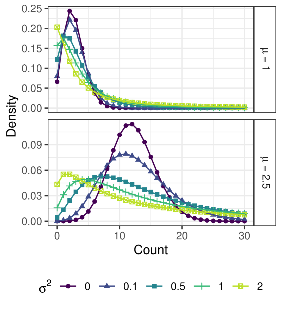
(a) Poisson Log-Normal.

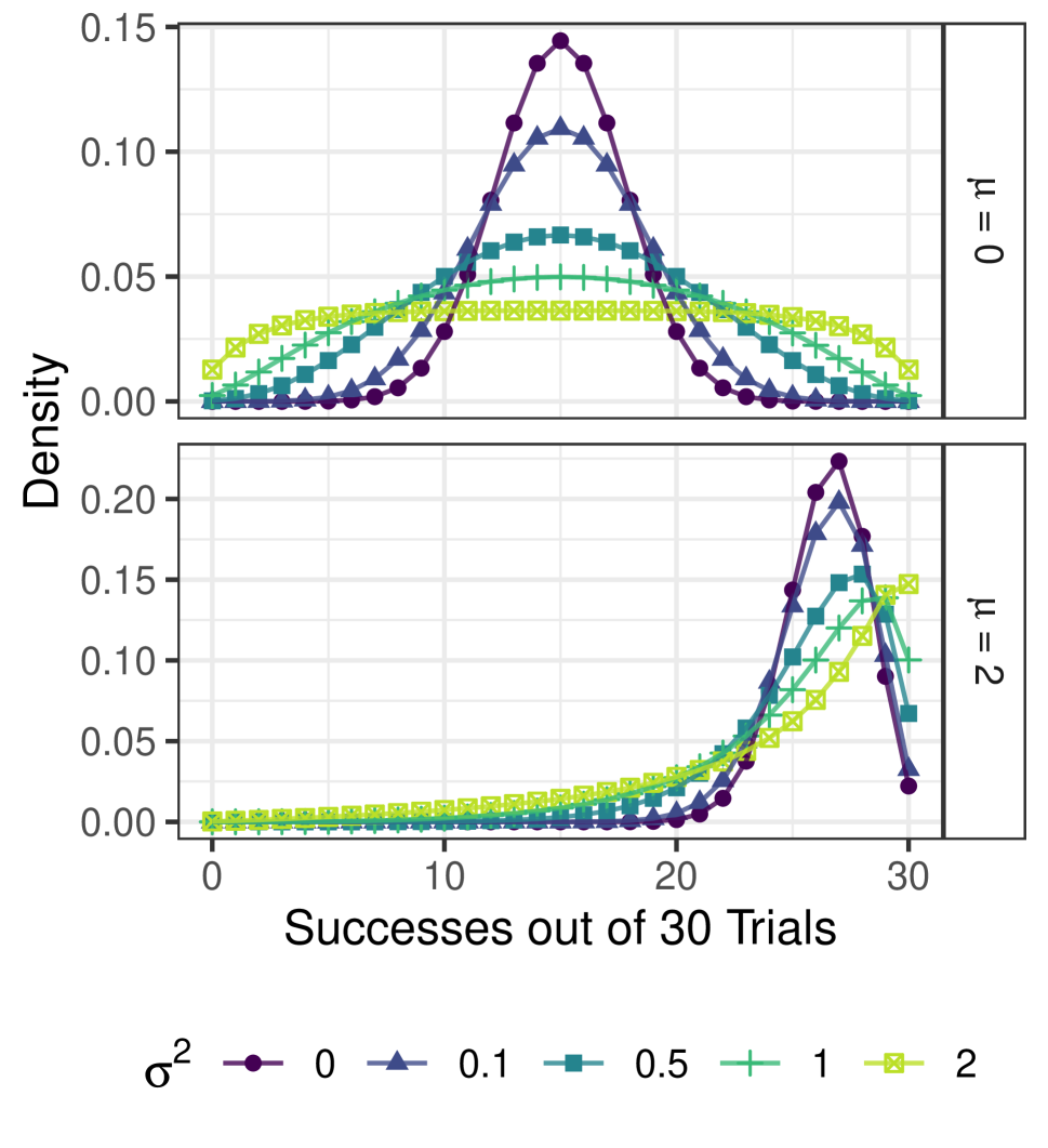
(b) Binomial Logistic Normal.

Fig. 1: Probability mass functions for random variables arising from a Poisson Log-Normal distribution $y\sim\mathcal{P}(e^{z}),z\sim\mathcal{N}(\mu,\sigma^{2})$ (left) and a Binomial Logistic Normal distribution $y\sim\text{Bin}(30,[1+e^{-z}]^{-1}),z\sim\mathcal{N}(\mu,\sigma^{2})$ (right).

2.1 Selected ULLGMs for Count Data Regression

Consider the PLN model, which applies to count-valued data and is based on a Poisson likelihood. The observed counts $y_{i}$ ($i=1,\dots,n$) are assumed to be Poisson distributed with an intensity parameter $\lambda_{i}$. In the standard, equi-dispersed, Poisson regression framework $\lambda_{i}$ is a deterministic function of observed covariates. In the presence of unobserved heterogeneity and overdispersion, it makes sense to assume that $\lambda_{i}$ is random, arising from an appropriate mixing distribution. Commonly considered mixing distributions include the Gamma distribution, which results in a negative binomial model (Greenwood and Yule, 1920), or an inverse Gaussian distribution which was used in Dean et al. (1989). A Log-normal mixing distribution model has appeared as such in the literature: Bulmer (1974) uses this mixture model in a location-scale context, which was extended to a multivariate setting in Aitchison and Ho (1989). The regression structure as used here was mentioned in Hinde (1982) and used in Tsionas (2010) in a Bayesian setting.

For the PLN model as in Table 1, we can show that

$$\begin{split}\mathbb{E}(y_{i}|\bm{x}_{i})&=e^{\alpha+\bm{x}_{i}^{\prime}\bm{\beta}+0.5\sigma^{2}}\\ \mathbb{V}(y_{i}|\bm{x}_{i})&=\mathbb{E}(y_{i}|\bm{x}_{i})+\mathbb{E}^{2}(y_{i}|\bm{x}_{i})(e^{\sigma^{2}}-1),\end{split}$$ (3)

allowing for overdispersion since $\mathbb{E}(y_{i}|\bm{x}_{i})<\mathbb{V}(y_{i}|\bm{x}_{i})$. The expression for the expected value further shows that the PLN model maintains a simple and intuitive interpretation of the regression parameters $\bm{\beta}$, similar to a Poisson regression model. Note that the usual dispersion index

$$\mathbb{D}(y_{i}|\bm{x}_{i})=1+\mathbb{E}(y_{i}|\bm{x}_{i})(e^{\sigma^{2}}-1)$$ (4)

is a monotonous function of $\sigma^{2}$ taking values on all of $\Re_{+}$. With the exception of the BeC class, similar results hold for the other models in Table 1, which gives $\sigma^{2}$ the interpretation of a dispersion parameter, controlling excess dispersion beyond the one implied by $F$. 1(a) shows example probability mass functions (pmfs) for the PLN model.

The BiL model represents another important member of the ULLGM family, generalising a Binomial model. To address overdispersion, it employs a logistic-normal distribution for the success probabilities of individual observations (Aitchison and Shen, 1980). Illustrations of pmfs of Binomial logistic normal distributions are provided in 1(b), underscoring the role of $\sigma^{2}$ as overdispersion parameter. BiL regression constitutes a highly flexible alternative to Beta-Binomial regression models for the analysis of overdispersed binomial outcomes. Although analytical expressions for the moments $\mathbb{E}(y_{i}|\bm{x}_{i},N_{i})$ and $\mathbb{V}(y_{i}|\bm{x}_{i},N_{i})$ are not known for a logistic link function, approximate results can be derived, such as

$$\mathbb{E}(y_{i}~{}|~{}\bm{x}_{i},N_{i})=N_{i}~{}\mathbb{E}[\pi_{i}]\approx N_{i}~{}\Phi\left(\frac{b(\alpha+\bm{x}^{\prime}_{i}\bm{\beta})}{\sqrt{1+b^{2}\sigma^{2}}}\right)$$ (5)

for a suitable value of $b>0$, where $\Phi(\cdot)$ is the cdf of a standard Gaussian random variable. Full details and an approximation of the variance are provided in Appendix A1. From (5), the interpretation of the coefficients and error variance is intuitive in the BiL model. As the value of $\sigma^{2}$ increases, the impact of the coefficients $\bm{\beta}$ is more muted. Also, $\mathbb{V}(y_{i}|\mu,\sigma^{2},N_{i})$ can be shown to approach the usual binomial variance $N_{i}\pi_{i}(1-\pi_{i})$ for $\sigma^{2}\rightarrow 0$. Similarly, the dispersion index $\mathbb{V}(y_{i}|\mu,\sigma^{2})/\mathbb{E}(y_{i}|\mu,\sigma^{2})$ tends to the binomial dispersion index $(1-\pi_{i})$ for $\sigma^{2}\rightarrow 0$, but is larger than the binomial dispersion index when $\sigma^{2}>0$, as also shown in Fig. A1; see Sec. A1 for more details.

2.2 Advantages of the ULLGM class

As previously discussed, for most underlying distributions $F$, the ULLGM specification intuitively allows for overdispersion, which is regulated by the extra parameter $\sigma^{2}$ in (2). In regression analysis, failing to account for overdispersion can lead to an underestimation of the standard errors. In the context of model selection and model averaging, ignoring overdispersion can lead to a preference for overly complex models, which compensate for the inability to account for the extra variation in the outcome. This undesirable phenomenon is illustrated for Poisson and Binomial regression models in Supplementary Sec. A3.

In addition, the structure of the models in the ULLGM class in (1) and (2) has a number of theoretical and practical benefits. Firstly, in the context of model uncertainty, the tractability of the Gaussian distribution lends itself to convenient applications of standard BMA methods. In particular, the parameters $\alpha,\bm{\beta}$ and $\sigma^{2}$ can be integrated out analytically with a popular and convenient prior, conditionally on $z_{i}$. This greatly simplifies the computational implementation (see Section 5) as well as the characterisation of posterior existence under this improper prior (see Section 4.1). The computational implementation is simple, allows for exact inference, and is significantly more flexible (e.g., accommodating situations where $n<p$) and often more efficient than related approximate and exact model averaging tools for generalized linear models (GLMs). In addition, the computational strategy can easily be modified to accommodate other members of the ULLGM class.

For specific ULLGM models, anecdotal empirical evidence suggests that relying on Gaussian error terms in the latent linear specification often provides superior model fits compared to allowing for overdispersion using non-Gaussian terms, such as log-Gamma errors in negative binomial regression models (Winkelmann, 2008; Tsionas, 2010). The Gaussian latent specification also holds theoretical merit, as normal error terms can be justified by a central limit theorem, if they capture a sum of latent shocks to the linear predictor. Finally, ULLGMs possess great potential for relatively straightforward generalization to multivariate settings with correlated observations (Aitchison and Ho, 1989; Chib and Winkelmann, 2001).

Certain limiting cases of ULLGM models are closely related to Gaussian regression models. For example, as $y_{i}\rightarrow\infty$, the PLN model converges to a Gaussian regression model with outcome $\log(y_{i})$. Similarly, as $N_{i}\rightarrow\infty$, the BiL model converges to a Gaussian regression model with the outcome $\text{logit}(y_{i}/N_{i})$, see Sec. A4 for further discussion. However, the ULLGM class has a number of key benefits compared to such Gaussian approximations. For example, ULLGMs do not rely on (potentially crude) approximations, provide valid uncertainty quantification and can naturally handle zero outcomes.

2.3 Model uncertainty

Given the model class defined in (1) and (2), the goal is to design a theoretical framework and a computational strategy for posterior and predictive inference, in the face of model uncertainty. Specifically, we are interested in model uncertainty with respect to inclusion and exclusion patterns of the components of the regression coefficient vector $\bm{\beta}$. Models will thus be characterized by the inclusion or exclusion of any of the columns of $\bm{X}$, which is the $n\times p$ matrix with $\bm{x}_{i}^{\prime}$ as its $i$th row. We denote the total number of potential covariates in $\bm{X}$ by $p$ while $p_{k}$ indicates the number of covariates from $\bm{X}$ that are included in model $M_{k}$. An intercept term is included in all models. This gives us a model space with $K=2^{p}$ elements and for model $M_{k}$ the distribution of $\bm{z}=(z_{1},\dots,z_{n})^{\prime}$ now becomes

$$\bm{z}|\alpha,\bm{\beta}_{k},\sigma^{2},M_{k}\sim\mathcal{N}(\alpha\bm{\iota}_{n}+\bm{X}_{k}\bm{\beta}_{k},\sigma^{2}\bm{I}_{n}),$$ (6)

where $\bm{\iota}_{n}$ is a column vector of $n$ ones, $\bm{I}_{n}$ is the $n$-dimensional identity matrix, $\bm{X}_{k}$ consists of the $p_{k}$ columns of $\bm{X}$ that correspond to the regressors that are included in $M_{k}$ and $\bm{\beta}_{k}$ groups the corresponding regression coefficients. The regressors in $\bm{X}$ are standardized by subtracting their means, which makes them orthogonal to the intercept and renders the interpretation of the intercept common to all models.

2.4 ULLGMs with random $r$

Sofar, we have focused on inference on the scalar observation-specific parameter, represented by $h(z_{i})$ for observation $i$. We now consider situations where we also want to conduct inference on other parameters added to the model, grouped in $r$ and common to all observations. We will assume that $r$ is a priori independent of $\bm{z}$ given a model within the set of models described in subsection 2.3:

$$r\amalg\bm{z}|M_{k},\text{for all }M_{k}.$$ (7)

Examples are the NBL and ErLN models, where we now allow $r$ to be an unknown parameter on which we conduct inference, rather than simply fixing it. In these models, $r$ is an integer scalar and it would be natural to assume (7) holds.

3 Prior Specification

We will focus on the prior setup that is most often encountered in the context of BMA. For the linear regression model in (6) taken in isolation, this prior satisfies many of the desiderata of Bayarri et al. (2012) for objective priors, such as measurement and group invariance and exact predictive matching. Specifically, we assume an improper, ’non-informative’ prior on the parameters common to all models

$$p(\alpha,\sigma^{2})\propto{\sigma^{-2}},$$ (8)

which is a convenient prior that has the advantage of being invariant with respect to rescaling and translating the $z_{i}$s. For the regression coefficients $\bm{\beta}_{k}$, we adopt a so-called $g$-prior which is invariant under affine linear transformations of the covariates

$$\bm{\beta_{k}}|\sigma^{2},M_{k}\sim\mathcal{N}(0\bm{\iota}_{p_{k}},g\sigma^{2}(\bm{X}_{k}^{\prime}\bm{X}_{k})^{-1}),$$ (9)

where $g>0$. Throughout, we will assume that the matrix formed by adding a column of ones to $\bm{X}_{k}$ is of full column rank. If the model space contains models for which this is not the case (for example because $p_{k}\geq n$), we will assign prior probability zero to those models. The scalar $g$ can either be fixed or assigned a hyperprior $p(g)$ as described in, e.g., Liang et al. (2008) or Ley and Steel (2012). We will consider both fixed and random $g$ when illustrating the framework in later sections. For BMA or model selection we require well-defined pair-wise Bayes factors between all models in the model space. In case a hyperprior is specified on $g$, it is necessary to take into account that $g$ does not appear in the null model (with $p_{k}=0$). Hence, a proper $p(g)$ is necessary in order to ensure meaningful model comparisons. For the null model with no regressors and only an intercept, the prior will simply be (8). Components of $\bm{\beta}$ that correspond to excluded regressors under $M_{k}$ are assigned a prior point mass at zero for that model.

As a prior on the model space, we employ the beta-binomial structure of Brown et al. (1998a), Ley and Steel (2009) and Scott and Berger (2010), which amounts to using a Beta$(a,b)$ prior on the common prior inclusion probability for each covariate and results in

$$P(M_{k})=\frac{\Gamma(a+b)}{\Gamma(a)\Gamma(b)}\frac{\Gamma(a+p_{k})\Gamma(b+p-p_{k})}{\Gamma(a+b+p)}.$$ (10)

This type of prior is less informative in terms of model size than fixing the prior inclusion probability of the covariates. Following the suggestions of Ley and Steel (2009), we choose $a=1$ and $b=(p-m)/m$, where $m$ is the prior expected model size. This means that the user only needs to specify a value for $m$. If there are any additional parameters $r$ as in Subsection 2.4, we specify a proper prior on $r$, satisfying (7).

4 Posterior Results

If we combine the $g$-prior setup proposed in Section 3 with the sampling model in (1) and (6), the conditional posterior distributions and the marginal likelihoods of the latent data $\bm{z}$ can be easily derived. We summarize the posterior on the model parameters as follows:

$$\beta_{k}|\alpha,\sigma^{2},\bm{z},M_{k}\sim N\left(\delta(\bm{X}_{k}^{\prime}\bm{X}_{k})^{-1}\bm{X}_{k}^{\prime}\bm{z},\delta\sigma^{2}(\bm{X}_{k}^{\prime}\bm{X}_{k})^{-1}\right),$$ (11)

where $\delta=\frac{g}{1+g}$,

$$\alpha|\sigma^{2},\bm{z},M_{k}\sim N\left(\bar{z},\frac{\sigma^{2}}{n}\right),$$ (12)

with $\bar{z}=\frac{1}{n}\sum_{i=1}^{n}z_{i}$ and

$$\sigma^{-2}|\bm{z},M_{k}\sim\mbox{Gamma}\left(\frac{n-1}{2},\frac{1}{2}\left[\delta\bm{z}^{\prime}Q_{(\iota:X_{k})}\bm{z}+(1-\delta)(\bm{z}-{\bar{z}}^{\prime}\iota)^{\prime}(\bm{z}-{\bar{z}}^{\prime}\iota)\right]\right),$$ (13)

where $Q_{A}=I_{n}-\bm{A}(\bm{A}^{\prime}\bm{A})^{-1}\bm{A}^{\prime}$ for any matrix $\bm{A}$ of full column rank. Finally, the marginal likelihood under fixed $g$ is

$$p(\bm{z}|M_{k})\propto(1+g)^{\frac{n-1-p_{k}}{2}}\left[\{1+g(1-R_{k}^{2})\}(\bm{z}-{\bar{z}}\iota)^{\prime}(\bm{z}-{\bar{z}}\iota)\right]^{-\frac{n-1}{2}},$$ (14)

where $R_{k}^{2}$ is the coefficient of determination of $\bm{z}$ regressed on $\bm{X}_{k}$ (and an intercept) and the proportionality constant is the same for all models, including the null model for which $p(\bm{z}|M_{0})\propto\left[(\bm{z}-{\bar{z}}\iota)^{\prime}(\bm{z}-{\bar{z}}\iota)\right]^{-\frac{n-1}{2}}$. Under random $g$ with hyperprior $p(g)$, the marginal likelihood is

$$p(\bm{z}|M_{k})\propto\int_{0}^{\infty}(1+g)^{\frac{n-1-p_{k}}{2}}\left[\{1+g(1-R_{k}^{2})\}(\bm{z}-{\bar{z}}\iota)^{\prime}(\bm{z}-{\bar{z}}\iota)\right]^{-\frac{n-1}{2}}p(g)dg.$$ (15)

4.1 Posterior existence

The prior for each given model $M_{k}$ is improper, as can be seen from the prior specification on the common parameters shared by all models in (8). Thus, we need to make sure that the posterior distribution of the parameters in each model is well-defined in the sense that the marginal likelihood is a finite quantity for each possible value of the observations $y_{i}$. We can state the following for cases where the possible additional parameter $r$ is fixed:

Theorem 1: If we combine the sampling model in (1) and (6) (ULLGMs defined in Table 1) with the improper prior structure in (8) and (9), then the posterior is well-defined for any model $M_{k}$ in the model space, if and only if the matrix composed of a column of ones and $\bm{X}_{k}$ has full column rank and, in addition, the following condition holds:

• for the PLN and NBL models: at least two of the observations are nonzero;

• for the BiL model: at least two observations are nonzero and smaller than $N_{i}$, where $N_{i}$ is the number of trials for observation $i$;

• for the ErLN, LNN and LNLN models: we have at least two observations.

The ULLGM models based on Bernoulli sampling (the BeC models) do not allow for a posterior under the prior in (8) and (9).

Proof: See Appendix A5.

Theorem 1 provides necessary and sufficient conditions for all the models in Table 1 that are not based on Bernoulli sampling, and thus fully characterizes posterior propriety for these ULLG models.

For models where the additional parameter $r$ is treated as random as in Subsection 2.4, we can derive the following:

Theorem 2: If we combine the sampling model in (1) and (6) with the improper prior structure in (8) and (9), along with a proper prior on $r$, $p(r|M_{k})$ satisfying (7), then the posterior is well-defined for any model $M_{k}$ in the model space, if the corresponding model with $r$ fixed leads to a proper posterior and if, in addition

$$\int f(r)p(r|M_{k})dr<\infty,$$ (16)

where we have defined

$$f(r)\equiv\int\prod_{i\in\cal N}P(y_{i}|z_{i},r)dz_{i}.$$ (17)

Proof: See Appendix A6.

An immediate consequence of Theorem 2 is that the NBL model and the ErLN model with random $r$ have proper posteriors under any proper prior on $r$ respecting (7), since $f(r)$ is constant in $r$ for these models (see sections A5.2 and A5.4). The situation is quite different for the LNLN model where Appendix A6 shows that we can not conclude that posterior inference on $r$ can be conducted with the overall prior structure assumed here.

5 Computational Considerations and Implementation

For PLN models, traditional maximum likelihood methods can yield unreliable parameter estimates even in simple scenarios, as highlighted in Tsionas (2010). As an alternative, Tsionas (2010) focuses on a Bayesian treatment of the univariate PLN regression setting, using an expectation-maximization algorithm for model estimation. MCMC estimation for the PLN model and extensions to $t$-distributed noise distributions are discussed in Chib and Winkelmann (2001). However, these contributions do not account for model uncertainty. Likewise, although estimation of BiL frameworks has been examined previously (Coull and Agresti, 2000), model uncertainty is typically not addressed.

The computational strategy we propose is based on the observation that, conditional on $z_{i}$, the posterior distributions of the latent Gaussian regression parameters, along with the marginal likelihoods and Bayes factors, assume a simple and convenient form. Hence, data augmentation, where the observed data is augmented with a posterior sample of $z_{i}$, is a natural choice for a posterior simulation strategy (Tanner and Wong, 1987). Given $z_{i}$, the parameters $\alpha$, $\bm{\beta}$, and $\sigma^{2}$ can then be updated using a simple Bayesian regression update.

To conduct inference under model uncertainty, we construct a partially collapsed Gibbs sampler over latent outcomes, regression parameters, and models. In particular, defining $\bm{\theta}=(\alpha,\bm{\beta},\sigma^{2})$, we iterate between drawing from $p(\bm{z}|\bm{\theta},\bm{y},M_{k})$ and from $P(\bm{\theta},M_{k}|\bm{y},\bm{z})=P(\bm{\theta},M_{k}|\bm{z})$ where the second step is composed of drawing from $P(M_{k}|\bm{z})$ and $p(\bm{\theta}|\bm{z},M_{k})$, which are both simple to simulate from. A similar blocking strategy for MCMC in latent Gaussian models is suggested in Geirsson et al. (2020). Details of the MCMC algorithm are summarized in Algorithm 1.

To obtain a sample of $z_{i}$, note that its conditional posterior distribution can be written as the product of a likelihood term defined via (1) and a Gaussian ’prior’ term (6). This factorization implies that the $z_{i}$s are all conditionally independent, given the remaining parameters and the data. Consequently, $n$ independent univariate updates can be performed, one for each $z_{i}$, in each iteration of the Gibbs sampler. To simulate from $p(z_{i}|\cdot)$, a simple strategy is to employ independent random-walk Metropolis-Hastings updates for all $i$. However, the simple structure of $p(z_{i}|\cdot)$ renders gradient-based methods a convenient and more efficient alternative. In the ULLGM framework, gradients of the likelihood and priors are typically available analytically and inexpensive to compute. We found that updating $z_{i}$ using an adaptive version of the Barker proposal from Livingstone and Zanella (2022) offers a good balance between mixing speed and robustness of the algorithm. Robustness is particularly important in certain ULLGMs, such as those involving the Poisson distribution, where gradient-based methods may exhibit numerical instabilities. The adaptive MCMC scheme we implement is based on diminishing adaptation rates, aiming for an acceptance probability of 0.57 for each $i$ (Roberts and Rosenthal, 2009). We provide the log posterior gradients of $z_{i}$ for selected models in Supplementary Sec. A7.

When $z_{i}$ is weakly identified by the likelihood, the proposed data augmentation scheme can induce some autocorrelation in the posterior draws. Nonetheless, the proposed algorithm is straightforward to implement and strikes a favorable balance between computation time and sampling efficiency. Moreover, it integrates effortlessly into the standard BMA framework. In contrast, conventional posterior simulation algorithms for high-dimensional non-Gaussian regression models often encounter significant difficulties, such as low sampling efficiency, expensive repeated likelihood evaluations, or the necessity for complex algorithmic techniques like Hamiltonian Monte Carlo. Extending conventional non-Gaussian regression model algorithms to handle model uncertainty efficiently is also challenging, as gradient-based methods can struggle with discrete sampling spaces, motivating approximate methods or intricate and computationally intensive reversible jump MCMC algorithms. In comparison, the ULLGM framework only requires very basic algorithmic techniques and knowledge of model averaging in linear Gaussian models, making it a simpler and more accessible approach while not relying on approximations. In addition, it allows for an easy adaptation of the general sampler in Algorithm 1 to accommodate specific members of the ULLGM class, simply by modifying the update of the latent variables $\bm{z}$.

For model proposals, we utilize an add-delete-swap (ADS) algorithm where each iteration involves adding, deleting, or swapping variables to create a new model proposal. This method has proven effective for the scenarios we examined. For very high-dimensional applications, future research might extend adaptive model proposals as suggested in Zanella (2020), Griffin et al. (2021), and Liang et al. (2023) to the ULLGM context. Details on the ADS proposal can be found in Sec. A8.

Algorithm 1 MCMC Sampling Procedure for fixed $r$ and $g$

1:Initialize model $M_{k}$, latent outcomes $\bm{z}$ and parameters $\sigma^{2}$, $\alpha$, $\bm{\beta_{k}}$

2:for each iteration do

3:     Update latent outcomes $\bm{z}$

4:           Sample from $p(\bm{z}|\alpha,\bm{\beta_{k}},\sigma^{2},M_{k},\bm{y})$ ($n$ parallel univariate updates)

5:     Between-Model Step:

6:           Propose $M^{*}$ using an add-delete-swap proposal

7:           Compute $p(\bm{z}|M^{*})$ and $p(\bm{z}|M)$ using (14)

8:           Accept or Reject moving to $M^{*}$ using (10) and the acceptance probability

9:                       $\zeta=\min\left(1,\frac{p(M^{*})}{p(M_{k})}\times\frac{p(\bm{z}|M^{*})}{p(\bm{z}|M_{k})}\times\frac{q(M_{k}\mid M^{*})}{q(M^{*}\mid M_{k})}\right)$

10:     Within-Model Step:

11:           Sample $\sigma^{2}$ from $p(\sigma^{2}|\bm{z},M_{k})$ defined in (13)

12:           Sample $\alpha$ from $p(\alpha|\sigma^{2},\bm{z})$ defined in (12)

13:           Sample $\bm{\beta_{k}}$ from $p(\bm{\beta_{k}}|\bm{z},\sigma^{2},M_{k})$ defined in (11)

14:end for

Assuming $g$ is random requires only minor modifications to the MCMC scheme outlined above. Given a prior density $p(g)$, we follow Ley and Steel (2012) and construct a Gibbs sampler that jointly explores latent outcomes, regression parameters, models, and values of $g$. This entails, in addition to the ’within-model’ update steps for $\alpha$, $\bm{\beta}$, and $\sigma^{2}$, simulating a new value of $g$. We use a univariate Metropolis-Hastings step with proposal mechanism $\log(g^{*})\sim\mathcal{N}\left(\log(g),\tau_{g}\right)$. The corresponding acceptance probability involves the prior $p(g)$, the marginal likelihood in (14), and the appropriate Jacobian, accounting for the proposal on the log-scale, and is given by $\min\left(1,\frac{p(g^{*})}{p(g)}\times\frac{p(\bm{z}|M_{k},g^{*})}{p(\bm{z}|M_{k},g)}\times\frac{g^{*}}{g}\right)$. Similar to the adaptive approach for $z_{i}$, the $g$ update utilizes adaptive MCMC techniques, aiming for an acceptance rate of $0.234$. Consequently, the Gibbs sampler is fully automatic, requiring no manual input beyond the initial prior specification. Finally, if additional auxiliary parameters are involved, the MCMC scheme can be expanded to a Gibbs sampler that jointly explores latent variables, regression parameters, models, $g$, and auxiliary parameters. These auxiliary parameters will typically be univariate or low-dimensional, rendering further (adaptive) Metropolis steps a viable sampling strategy.

6 Applications to Simulated Data

To assess the effectiveness of the PLN and BiL model averaging algorithms, we used simulated data, varying both the number of observations ($n=150$ and $1,000$) and the number of regressors ($p=50$ and $100$), while using $N_{i}=30$ for the BiL model. In all scenarios, the linear predictor was defined as $1.5+\bm{x}_{i}^{\prime}\bm{\beta}^{\star}$, where the first ten regression coefficients were non-zero. The coefficients were specified as:

$$\bm{\beta}^{\star}=\frac{\log(p)}{\sqrt{n}}(2,-3,2,2,-3,3,-2,3,-2,3,0,\ldots,0)^{\prime}\in\mathbb{R}^{P}.$$

The regressors $\bm{x}_{i}$ were drawn from a normal distribution with mean 0 and covariance matrix $\Sigma$, where $\Sigma_{jk}=\rho^{|j-k|}$, determined by a correlation coefficient $\rho$. We used $\rho=0.6$ in our examples, representing a challenging setting with relatively high correlation among the regressors.

To test the resilience against misspecification, we utilized three different DGPs to generate the latent outcomes $z_{i}$. First, we added noise terms from $\mathcal{N}(0,\sigma^{2})$ with $\sigma^{2}=0.2$ to the linear predictor (the ULLGM case). In the second setting, we used a noise-free linear predictor ($\sigma^{2}=0$), corresponding to a GLM setting. Finally, we added logarithmic samples from $\mathcal{G}(5.5,5.5)$ (a gamma distribution with mean one and variance $\frac{1}{5.5}$) as noise to the linear predictor. The implied error distribution has a variance of approximately 0.2, but is skewed and has a non-zero mean.

Regarding the prior setup, we choose $m=5$ to favor sparse models. We compared two settings for $g$. Firstly, a ’unit information prior’ that fixes $g=n$, a popular and empirically successful default in many BMA applications (Kass and Wasserman, 1995). The second setting accounts for theoretical shortcomings of fixed $g$ (Liang et al., 2008) by letting $g$ be random using a hyper-$g/n(a=3)$ prior, as favored in Ley and Steel (2012). For each of the 24 settings per model, we simulated 100 replicate data sets, collected several measures of accuracy – such as the Brier score, false positive and negative rates and expected model size – and averaged the results. In each model run, we collected 300,000 posterior samples after an initial burn-in of 250,000 iterations.

Detailed results of the simulation study are summarized in Table A1 in Appendix A9. They suggest a reasonably high level of accuracy across all settings. In general, the simulation results are in line with what one would expect, for instance increasing accuracy with increasing ${n}$. The simulation runs indicate that the ULLGM framework performs well, even in situations with challenging signal-to-noise ratios and in scenarios with misspecification of the sampling model, implying a certain level of robustness of the ULLGM framework for variable selection and model averaging. In terms of prior choices, we find the unit information prior to be slightly more robust in the settings we investigate, with the hyper-$g/n$ prior showing a tendency to favor slightly larger models. In general, a certain sensitivity of model averaging outcomes to prior settings is well documented in the literature and warrants a careful comparison of results based on a range of priors in applied contexts.

7 Real Data Applications

7.1 Measles Vaccination Coverage in Ethiopia

Vaccination coverage rates are a key metric for assessing the performance of national health and immunization systems. Such performance indicators are, however, generally measured using national statistics or at the scale of large regions. This is often due to the design of surveys, administrative convenience, or operational constraints. This approach can obscure subnational variations and ’coldspots’ of low coverage, potentially allowing diseases to persist even when overall coverage rates are high. Hence, to reduce health inequalities and make steps towards disease elimination targets, it is crucial to more accurately characterize fine-scale variations in coverage. Growing demand for subnational health metrics has led to significant interest in empirical models that provide regional vaccination coverage estimates, along with the uncertainties associated with these estimates (Utazi et al., 2018). These efforts often rely on Binomial models, which forms the basis of the BiL model in Table 1. These models typically incorporate a regression function and spatial smoothing mechanisms, but usually do not address model uncertainty.

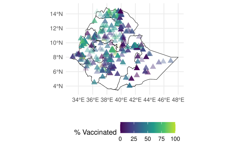
Fig. A6: Map of Survey Clusters in Ethiopia DHS Survey 2019. Cluster transparency is inversely proportional to local sample size.

Given the potential effectiveness of BMA as a predictive tool, we employ the BiL model to analyze data on vaccination coverage in Ethiopia. Specifically, we utilize data from the 2019 Demographic and Health Survey (DHS) in Ethiopia. The data is collected in survey clusters, with a cluster typically consisting of 25-30 households, representing for example a rural settlement or an urban neighborhood. The dataset includes a total of $n=305$ clusters. For each cluster, we record $y_{i}$, the number of children born in the three years before the survey who have received the first dose of a measles (or measles-containing) vaccine, out of $N_{i}$, the total number of children born within the same period whose vaccination status is known. The observed vaccination rates $y_{i}/N_{i}$ within these clusters vary from 0% to 100%, with an average rate of 44.8% across all clusters. A map illustrating the distribution of survey clusters across Ethiopia and their respective sample estimates of vaccination coverage rates is presented in Supplementary Fig. A6. On this map, clusters with lighter coloring indicate a smaller local sample size $N_{i}$, implying a smaller influence of cluster $i$ on the BiL parameter estimates.

We gather a set of $p=63$ potentially relevant predictors of vaccination rates and apply BMA to identify a robust subset of determinants. The covariates include a variety of factors that are related to health outcomes, such as regional sociodemographic characteristics, household living standards, and proxies for local economic development like a satellite-based nightlight intensity measure. Additionally, the covariates cover climatic conditions, measures of accessibility of different regions, and several nutritional scores based on anthropometric measurements of children in the survey clusters. To account for latent spatial variation in vaccination rates, we also incorporate indicators for Ethiopia’s 11 regions and GPS-based data on the clusters’ latitude, longitude, and altitude. This set of covariates encompasses a range of variables that can be found in most DHS surveys or can be collected from publicly accessible sources. Therefore, this analysis might hold broader interest beyond the Ethiopian case study presented here. Detailed information on the full set of covariates, along with summary statistics, is provided in Supplementary Table A2.

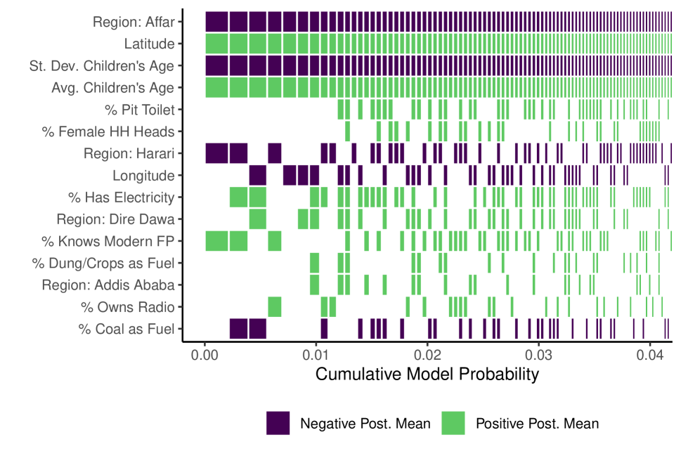
(a) Highest Probability Models.

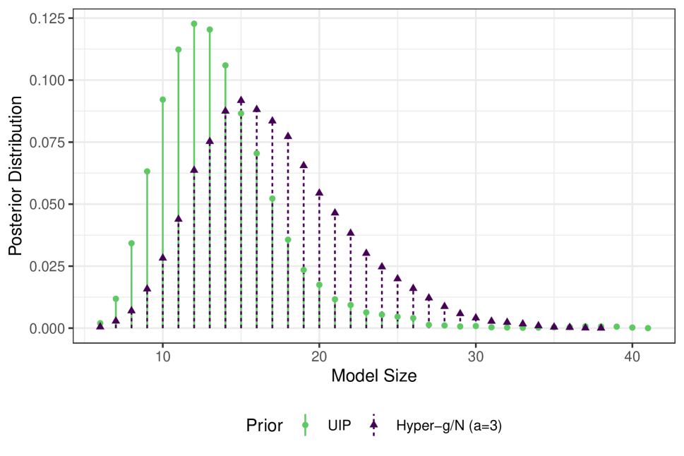
(b) Posterior Distribution of Model Size.

Fig. 2: Estimation Results (Measles Vaccination Data). Highest probability models plot includes variables with estimated $\text{PIP}>0.3$ under unit information prior.

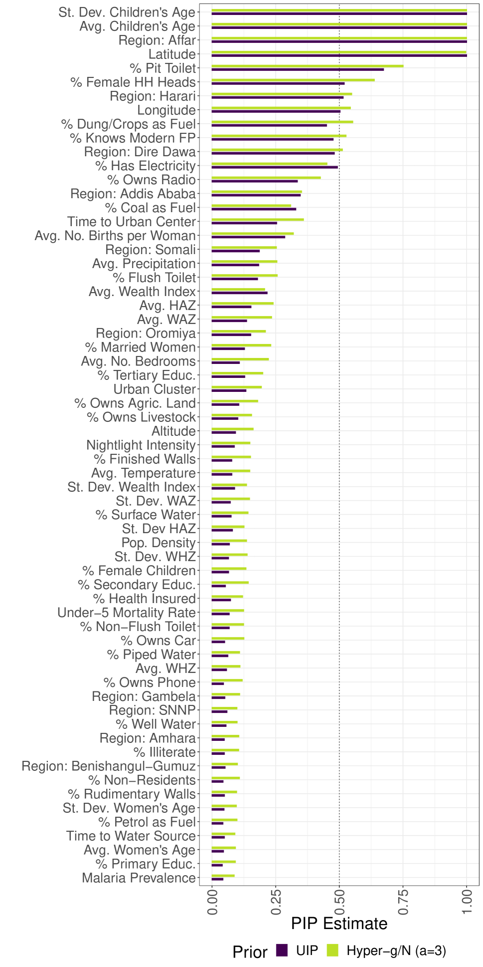
(a) Post. Inclusion Probabilities.

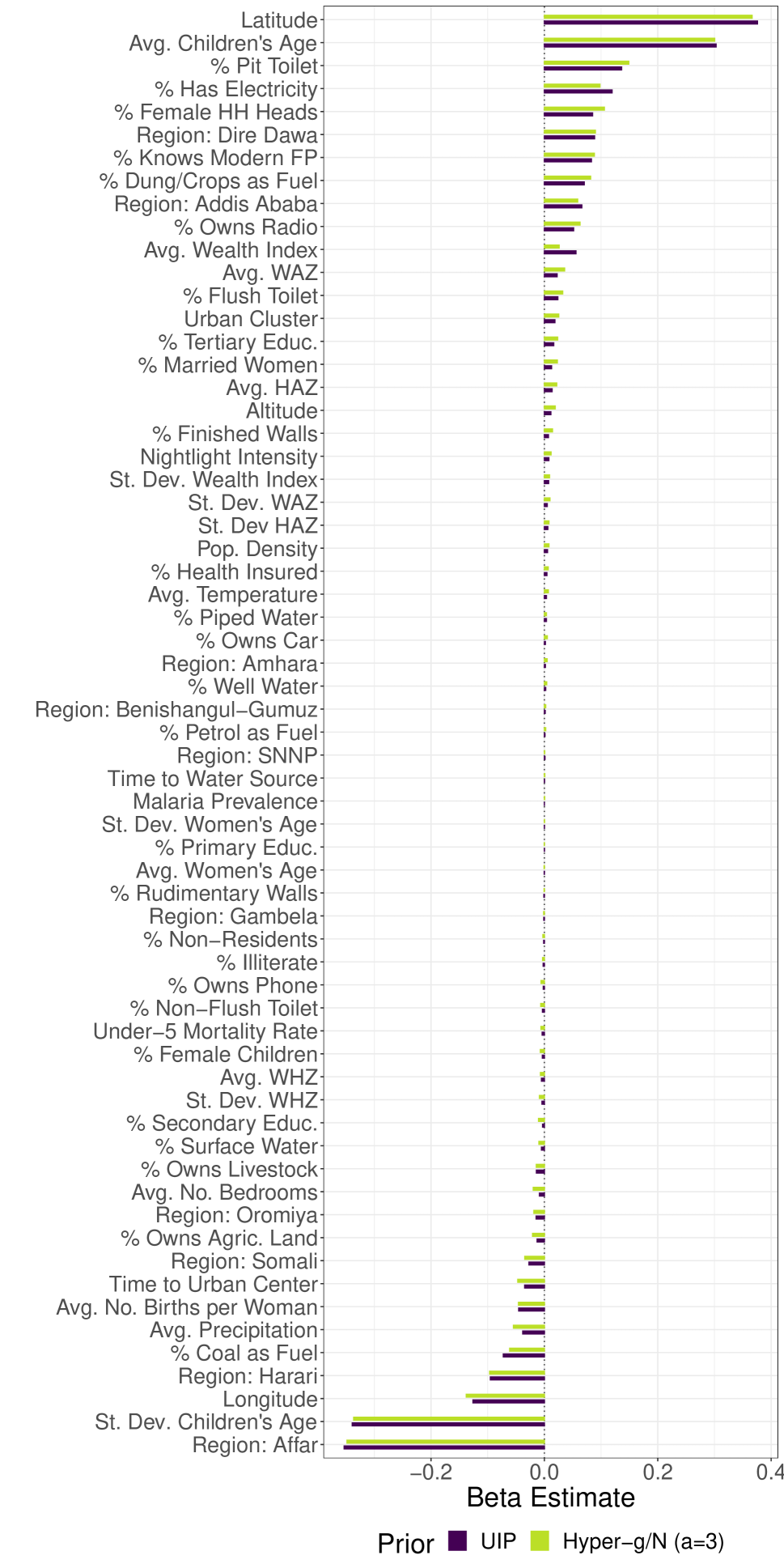
(b) Coefficient Post. Means.

Fig. A7: Estimation Results for Measles Vaccination Data.

We implement the BiL model using the algorithm described in Section 5, under a UIP prior ($g=n$) and a hyper-$g/n$ ($a=3$) prior, alongside an agnostic uniform prior on model size ($m=p/2$). The analysis is based on $300,000$ posterior draws, collected following a burn-in phase of $250,000$ iterations. We provide the estimated posterior inclusion probabilities and posterior means of $\bm{\beta}$ in Supplementary Fig. A7. Under both priors, the posterior means of the intercept are $\mathbb{E}({\alpha}|\bm{y})=-0.28$ while $\mathbb{E}({\sigma}^{2}|\bm{y})=0.17$ under the unit information prior and $\mathbb{E}({\sigma}^{2}|\bm{y})=0.23$ under the hyper-$g/n$ prior. 2(a) shows the highest probability models under the unit information prior, while 2(b) illustrates the posterior distributions of model size, indicating a slight preference for larger models under the hyper-$g/n$ prior (which tends to lead to somewhat smaller values for $g$). The median probability models, which include those covariates with a posterior inclusion probability (PIP) greater than $0.5$, agree on eight influential variables. The average age of children in a cluster is strongly positively associated with vaccination rates, likely due to increased interactions with healthcare systems over time and the fact that vaccines are typically not scheduled for administration directly after birth, decreasing the likelihood of very young children being vaccinated. Conversely, a larger standard deviation in children’s ages within a cluster, indicating a more dispersed age distribution, is significantly associated with lower vaccination rates, suggesting that age homogeneity can enhance the effectiveness of health interventions and vaccination campaigns. Such uniformity may support more targeted health education and vaccination efforts, encourage communal sharing of health information, and enable healthcare providers to better plan and deliver vaccination services to the predominant age group, thereby boosting overall coverage. The significant positive relationship between latitude and vaccination rates suggests higher coverage in northern clusters, while the pronounced negative impact of being in the Affar region—characterized by remoteness, pastoralist communities and regional political tensions — indicates unobserved factors affecting spatial variations in vaccination rates. Model probabilities are in general relatively spread out, reflecting a rather high amount of collinearity among the covariates. The highest probability models are detailed in Supplementary Table A4 and Table A5. Numerical results on estimated posterior means, standard deviations, and inclusion probabilities are available in Supplementary Table A3.

7.2 Bilateral Migration Flows Between OECD Countries

We use the PLN model to examine migration flows between the 38 OECD countries from 2015 to 2020. This challenging dataset comprises $n=1,406$ bilateral migration flows, ranging from zero to 1.6 million migrants, leading to a dispersion index of 345,000. BMA is conducted with a set of $p=54$ potentially important covariates and results are presented in Appendix A10.

7.3 Comparative Predictive Performance

To understand the predictive capabilities of ULLGMs, we carried out a predictive exercise based on the measles vaccination data and the migration data. Each data set was randomly split into test (prediction) and training sets 100 times, with 15% allocated to the test set and the remaining 85% to the training set. Then, we estimated models using the training data and evaluated their prediction accuracy on the test data. For the ULLGMs, a unit information prior and a hyper-$g/n$ prior were used. Non-BMA versions of ULLGMs were estimated as well, including the full, null, median probability, and highest probability models, based on the unit information prior BMA results. For the bilateral migration data, we also performed a Poisson regression BMA analysis using adaptations of the AutoRJMCMC algorithm of Lamnisos et al. (2009). In addition, the full, null, median probability, and highest probability models, based on the AutoRJMCMC results were included in the analysis. For the vaccination data, we added Binomial logistic regression models without overdispersion using BMA and also considering the full, null, median, and highest posterior models. For BMA methods, we set $m=p/2$ to stay agnostic about model size a priori. In the case of the GLM models, we used $\alpha\sim\mathcal{N}(0,1000)$ and $\bm{\beta_{k}}|M_{k}\sim\mathcal{N}(0\bm{\iota}_{p_{k}},g(\bm{X}_{k}^{\prime}\bm{X}_{k})^{-1})$ as priors on the regression parameters. For each model, we collected 300,000 posterior samples after an initial burn-in period of 250,000 iterations. For posterior simulation under Binomial and Poisson GLMs, we employed a multivariate Gaussian posterior approximation, derived from a Bayesian IWLS algorithm (Gamerman, 1997).

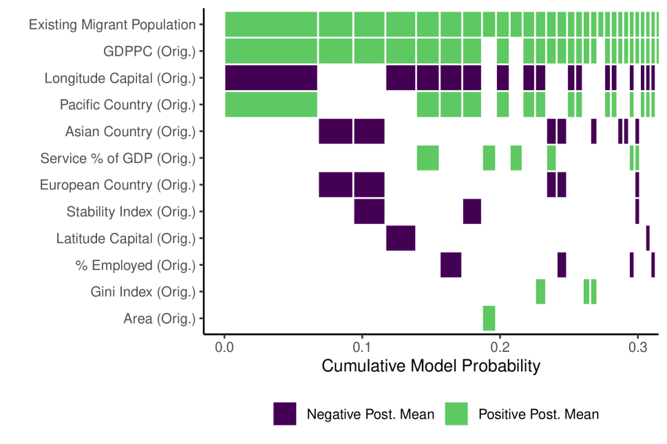
(a) Highest Probability Models.

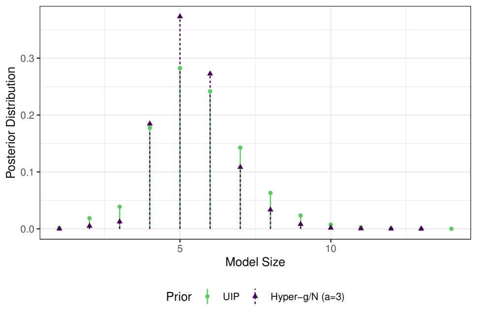
(b) Posterior Distribution of Model Size.

Fig. A10: Estimation Results (Austrian Migration Flow Data Subset). Highest probability models plot includes variables with estimated $\text{PIP}>0.1$ under unit information prior.

In addition to analyzing the full samples, we performed leave-one-out cross-validation on subsamples of the data sets to gain insights into predictive performance in smaller samples. For the migration data, we examined the $n=38$ migration flows from OECD countries to Austria, excluding all destination-specific and three multicollinear covariates (resulting in $p=28$). For the vaccination data, we considered the data for the three regions with the lowest vaccination rates ($n=85$, $p=54$). Given the small sample size, we expect sparser models to be relevant a priori, and set $m=5$ to slightly favor smaller models. Graphical summaries of the BMA results for these subsamples, comparable to those presented in Sec. 7.1 and Sec. A10, are provided in Supplementary Figures A10 to A13.

For predictive evaluation, we employ the logarithmic score or log predictive score (LPS, see e.g. Fernández et al., 2001), which is a proper scoring rule for counts (see Czado et al., 2009). Denoting the training data as $\bm{y}^{\text{t}}$ and the holdout data to be predicted as $\bm{y}^{\text{p}}$ with $n_{p}$ elements $y^{\text{p}}_{i}$ and associated covariate values $\bm{x}^{\text{p}}_{i}$, LPS is defined as

$$\text{LPS}=-\frac{1}{n_{p}}\sum_{i=1}^{n_{p}}\log P(y^{\text{p}}_{i}~{}|~{}\bm{x}^{\text{p}}_{i},\bm{y}^{\text{t}}).$$ (18)

The required posterior predictive probabilities evaluated at the holdout counts are approximated as detailed in Supplementary Sec. A11.

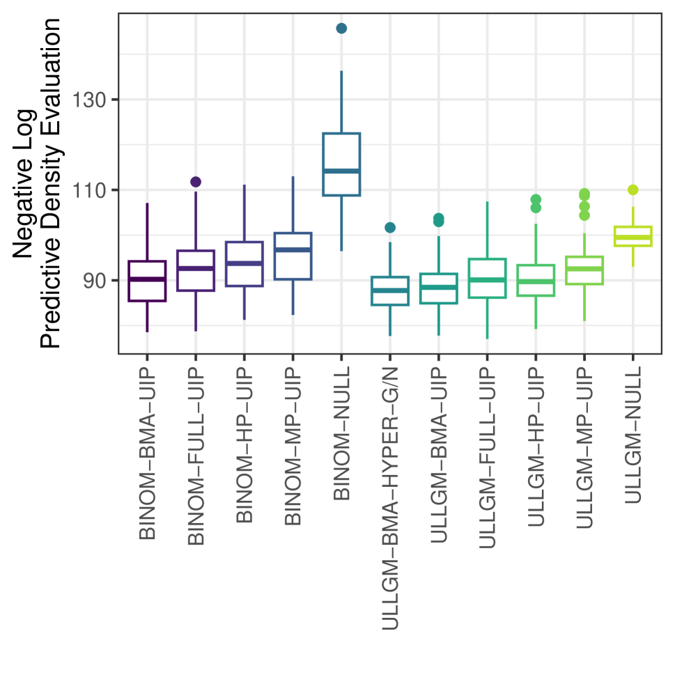
(a) Full Vaccination Data (All Models).

(b) Full Migration Data (All Models).

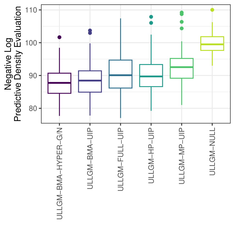
(c) Full Vaccination Data (ULLGM Models).

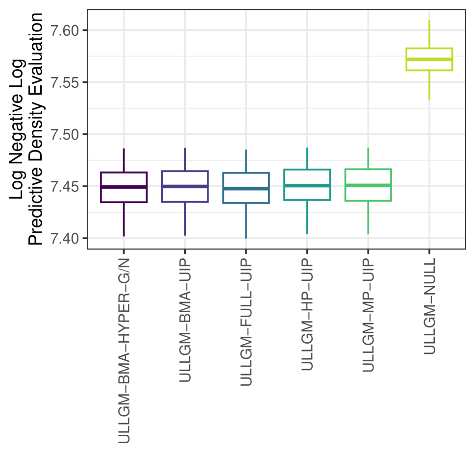
(d) Full Migration Data (ULLGM Models).

Fig. A14: Boxplots of log predictive density evaluations across 100 random training-test partitions for the full data sets. For the migration data, the results are on a double log scale.

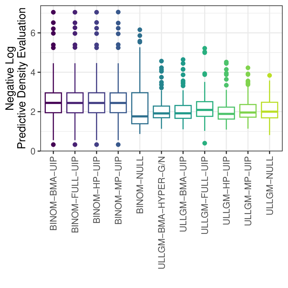
(a) Subset Vaccination Data (All Models).

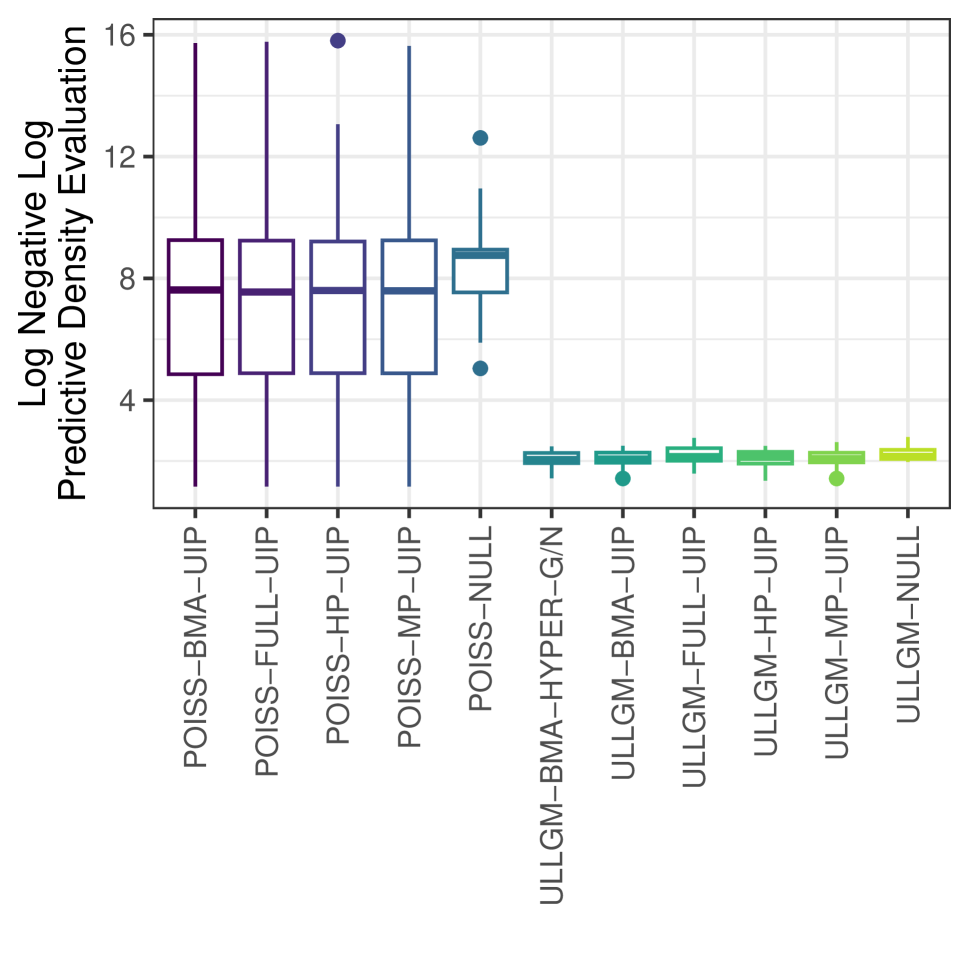
(b) Subset Migration Data (All Models).

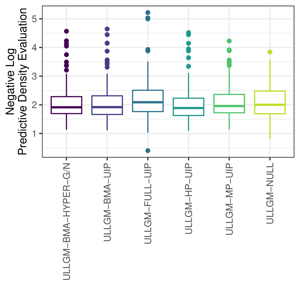
(c) Subset Vaccination Data (ULLGM Models).

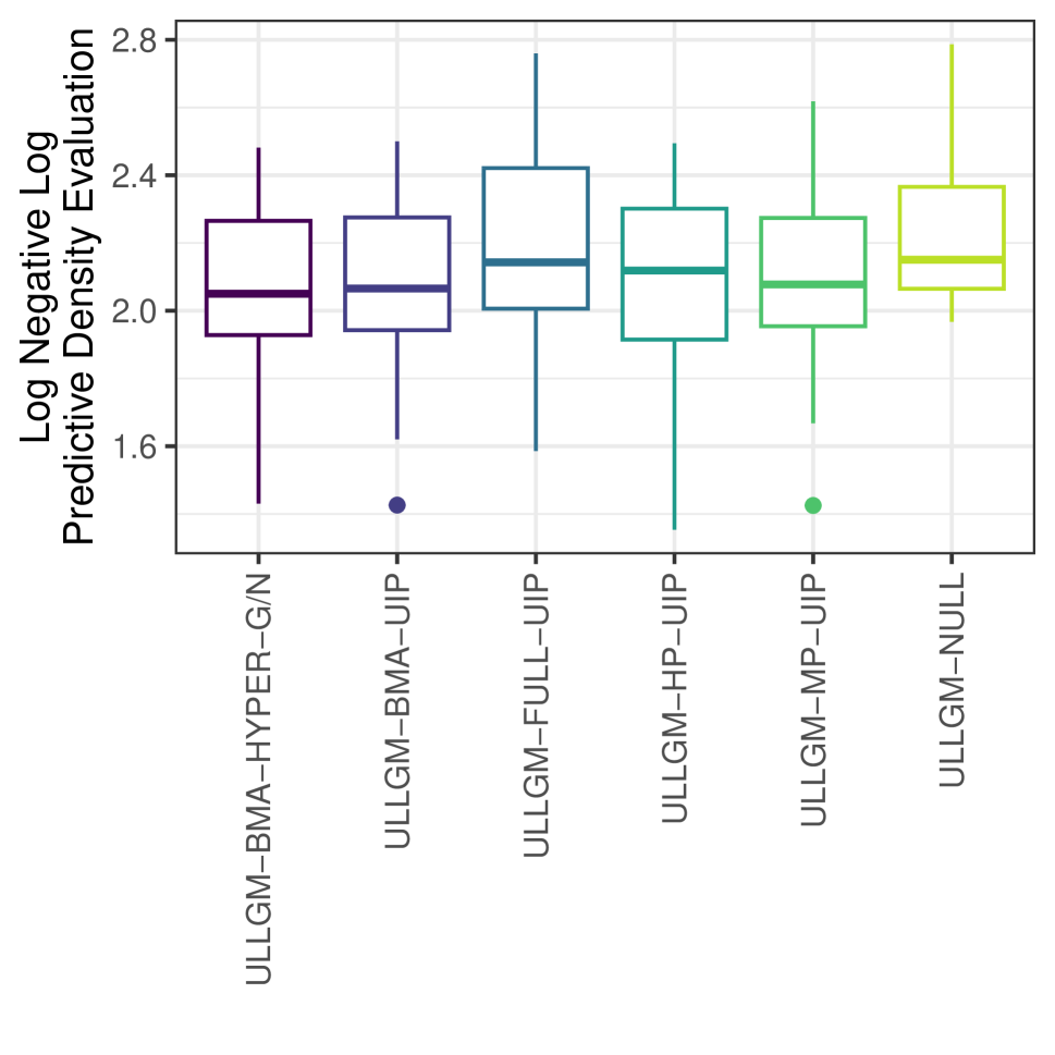
(d) Subset Migration Data (ULLGM Models).

Fig. A15: Boxplots of log predictive density evaluations based on leave-one-out cross-validation in the reduced samples. For the migration data, the results are on a double log scale.

The results are presented in Table 2. Smaller values of LPS indicate better predictive performance. The mean, median, minimum, and maximum scores for each model across 100 partitions, as well as the share of replications where a model ranked as the best or worst, along with its average ranking are provided. Additionally, for the ULLGMs, average posterior means for $\sigma^{2}$ are reported. The model size, indicating the posterior mean number of included regressors, is also documented, averaged over all partitions. Boxplots of the LPS across the 100 replications are provided in Supplementary Fig. A14 and Fig. A15.

Table 2: Results of Predictive Exercise (best performance in bold).

	Avg. LPS	Med. LPS	Min. LPS	Max. LPS	% Best	% Worst	Avg. Rank	$\sigma^{2}$	Avg. Model Size
Full Vaccination Data (n=305)
ULLGM-BMA-HYPER-g/n	1.95	1.95	1.73	2.26	0.61	0.00	1.67	0.22	16.53
ULLGM-BMA-UIP	1.96	1.97	1.73	2.31	0.10	0.00	2.35	0.16	13.85
ULLGM-FULL-UIP	2.01	2.00	1.71	2.39	0.09	0.00	4.44	0.01	63
ULLGM-HP-UIP	2.01	1.99	1.76	2.40	0.05	0.00	4.59	0.25	7.44
ULLGM-MP-UIP	2.06	2.06	1.80	2.43	0.01	0.00	6.36	0.28	7.94
ULLGM-NULL	2.22	2.21	2.07	2.44	0.00	0.00	9.17	0.98	0
BINOM-BMA-UIP	2.01	2.01	1.75	2.38	0.09	0.00	4.30	0	14.32
BINOM-FULL-UIP	2.06	2.06	1.75	2.48	0.03	0.00	6.55	0	63
BINOM-HP-UIP	2.08	2.08	1.81	2.47	0.01	0.00	7.23	0	12.12
BINOM-MP-UIP	2.13	2.15	1.83	2.51	0.01	0.01	8.35	0	11.40
BINOM-NULL	2.56	2.54	2.14	3.24	0.00	0.99	10.99	0	0
Subset Vaccination Data (n=85)
ULLGM-BMA-HYPER-g/n	2.11	1.91	1.13	4.57	0.02	0.00	4.64	0.29	5.76
ULLGM-BMA-UIP	2.12	1.92	1.11	4.64	0.04	0.04	4.45	0.25	4.78
ULLGM-FULL-UIP	2.27	2.09	0.40	5.22	0.13	0.00	5.18	0.01	54
ULLGM-HP-UIP	2.08	1.89	1.09	4.52	0.15	0.02	4.39	0.39	1.00
ULLGM-MP-UIP	2.15	1.96	1.14	4.23	0.04	0.02	5.51	0.45	1.04
ULLGM-NULL	2.13	2.00	0.82	3.84	0.09	0.08	5.99	0.63	0
BINOM-BMA-UIP	2.69	2.45	0.33	7.05	0.04	0.14	7.76	0	53.99
BINOM-FULL-UIP	2.69	2.44	0.33	7.05	0.02	0.16	7.78	0	54
BINOM-HP-UIP	2.69	2.44	0.33	7.05	0.07	0.16	7.96	0	54.00
BINOM-MP-UIP	2.69	2.44	0.33	7.05	0.01	0.13	7.72	0	54.00
BINOM-NULL	2.29	1.76	0.87	6.16	0.41	0.24	4.64	0	0
Full Migration Data (n=1,406)
ULLGM-BMA-HYPER-g/n	8.18	8.18	7.80	8.49	0.19	0.00	1.93	0.73	31.30
ULLGM-BMA-UIP	8.19	8.19	7.81	8.50	0.03	0.00	2.86	0.72	28.13
ULLGM-FULL-UIP	8.18	8.17	7.79	8.48	0.71	0.00	1.65	0.69	54
ULLGM-HP-UIP	8.20	8.19	7.82	8.50	0.00	0.00	4.53	0.72	26.04
ULLGM-MP-UIP	8.20	8.20	7.82	8.50	0.07	0.00	4.03	0.72	26.84
ULLGM-NULL	9.25	9.25	8.90	9.61	0.00	0.00	6.00	6.82	0
POISS-BMA-UIP	$1.4\times 10^{3}$	$1.3\times 10^{3}$	$6.38\times 10^{2}$	$3.7\times 10^{3}$	0.00	0.00	8.35	0	54.00
POISS-FULL-UIP	$1.4\times 10^{3}$	$1.3\times 10^{3}$	$6.39\times 10^{2}$	$3.7\times 10^{3}$	0.00	0.00	8.56	0	54
POISS-HP-UIP	$1.4\times 10^{3}$	$1.3\times 10^{3}$	$6.39\times 10^{2}$	$3.7\times 10^{3}$	0.00	0.00	8.47	0	54.00
POISS-MP-UIP	$1.4\times 10^{3}$	$1.3\times 10^{3}$	$6.38\times 10^{2}$	$3.7\times 10^{3}$	0.00	0.00	8.62	0	54.00
POISS-NULL	$3\times 10^{4}$	$2\times 10^{4}$	$1\times 10^{4}$	$8\times 10^{4}$	0.00	1.00	11.00	0	0
Subset Migration Data (n=38)
ULLGM-BMA-HYPER-g/n	8.10	7.77	4.18	11.96	0.51	0.00	2.24	0.16	5.37
ULLGM-BMA-UIP	8.14	7.89	4.16	12.18	0.05	0.00	3.22	0.27	5.51
ULLGM-FULL-UIP	9.19	8.53	4.88	15.80	0.05	0.00	4.84	0.16	28
ULLGM-HP-UIP	8.33	8.32	3.87	12.11	0.22	0.00	3.03	0.26	3.95
ULLGM-MP-UIP	8.39	7.99	4.16	13.71	0.08	0.00	3.54	0.33	3.51
ULLGM-NULL	9.48	8.59	7.15	16.23	0.03	0.00	5.54	4.06	0
POISS-BMA-UIP	$2\times 10^{5}$	$2.0\times 10^{3}$	3.19	$7\times 10^{6}$	0.03	0.14	8.46	0	28.00
POISS-FULL-UIP	$2\times 10^{5}$	$1.9\times 10^{3}$	3.19	$7\times 10^{6}$	0.00	0.03	8.73	0	28
POISS-HP-UIP	$2\times 10^{5}$	$2.0\times 10^{3}$	3.19	$7\times 10^{6}$	0.03	0.19	8.54	0	28.00
POISS-MP-UIP	$2\times 10^{5}$	$2.0\times 10^{3}$	3.19	$6\times 10^{6}$	0.00	0.03	8.38	0	28.00
POISS-NULL	$1\times 10^{4}$	$6.3\times 10^{3}$	$1.54\times 10^{2}$	$3\times 10^{5}$	0.00	0.62	9.49	0	0

In the real data applications examined, ULLG models outperform their counterparts that do not account for overdispersion. For the vaccination data, overdispersion is moderate, resulting in relatively comparable outcomes for ULLGMs and non-ULLGMs. On average, the ULLGMs perform better. At the same time, they tend to select smaller models. We attribute this to the inability to accommodate the variability in the data without the overdispersion parameter: the standard models have to compensate by including more covariates. This effect is particularly pronounced in the migration data analysis, where substantial overdispersion in the data causes all coefficients in a standard Poisson regression model to appear as important predictors. Consequently, the RJMCMC-BMA algorithm for Poisson regression predominantly visits the full model. This still does not adequately capture the data dispersion, which results in overly concentrated predictive distributions and very suboptimal predictive performance. In contrast, ULLGMs can accommodate overdispersion through $\sigma^{2}$ and produce dramatically better predictive scores. Note that estimates for $\sigma^{2}$ are substantially higher for the null models (where all overdispersion has to be accommodated through $\sigma^{2}$) and lower for the full models. Among the ULLGMs, the hyper-$g/n$ prior tends to favor larger models, but provides similar or slightly better predictive performance compared to the unit information prior framework in both data sets. Irrespective of whether we use an LGM structure or not, the null models tend to predict badly, for all data sets. Thus, covariate information substantially improves prediction, empirically justifying the regression framework. The best overall performance is shown by the ULLGM-BMA model with a hyper $g/n$ prior which never predicts worst and predicts best in over 50% of the holdout samples for two of the four datasets considered.

8 Concluding Remarks

In this article, we present a formal and general framework for BMA in non-Gaussian regression models, based on the class of ULLGMs. We provide full characterisations of posterior existence for key models within this class and develop a simple, efficient and adaptable MCMC algorithm to handle posterior simulation under model uncertainty. Our empirical investigations focus on PLN and BiL regression models for overdispersed count data. A simulation study suggests high accuracy and robustness to likelihood misspecification, making the framework potentially useful in a wide range of settings. Finally, we apply the models to two real data applications and conduct a comparative predictive exercise, further illustrating the advantages of the proposed framework.

For the measles vaccination rate application, we deal with data that are often modeled using spatial methods. The migration data are essentially network data, models for which often include latent variables to capture similarities between the nodes. Here, we used simple regression models for both applications. The ability to use BMA allows us to include many potential predictors, which helps to explicitly capture structures that are usually treated as latent. This approach not only aids in interpretation and simplifies modeling but also enables us to predict observables using only the covariates. For some applications, combining BMA with latent variable modeling could provide an even more powerful framework. Adapting existing MCMC algorithms for latent variable models to incorporate model uncertainty is a natural extension of the algorithms developed here.

Several additional research directions are attractive avenues for future exploration. In terms of substantive applications, the proposed framework is broadly applicable and could be particularly valuable for analyzing model uncertainty in multi-way contingency tables (Ntzoufras et al., 2000) and related problems, such as multiple systems analysis (Silverman, 2020). Furthermore, many practically relevant applications of regression models involve multivariate outcomes. Combining multivariate latent Gaussian models with multivariate Bayesian variable selection techniques (Brown et al., 1998b) could yield very interesting modeling environments.

SUPPLEMENTARY MATERIAL

A1 Moments and Dispersion of $y_{i}$ under the BiL model

In order to approximate the first two moments of $y_{i}$ under the BiL model, we approximate the logistic cdf with a scaled Gaussian cdf, such that

$$\begin{split}\mathbb{E}(y_{i}~{}|~{}\bm{x}_{i},N_{i})&=N_{i}~{}\mathbb{E}(\pi_{i}~{}|~{}\bm{x}_{i})\\ &=N_{i}~{}\int\frac{\exp{(z_{i})}}{1+\exp{(z_{i})}}~{}\mathcal{N}(z_{i}~{}|~{}\alpha+\bm{x}_{i}^{\prime}\bm{\beta},\sigma^{2})~{}dz_{i}\\ &\approx N_{i}~{}\int\Phi(bz_{i})~{}\mathcal{N}(z_{i}~{}|~{}\alpha+\bm{x}_{i}^{\prime}\bm{\beta},\sigma^{2})~{}dz_{i}\\ &=N_{i}~{}\Phi\left(\frac{\alpha+\bm{x}^{\prime}_{i}\bm{\beta}}{\sqrt{b^{-2}+\sigma^{2}}}\right)=N_{i}~{}\Phi\left(\frac{b(\alpha+\bm{x}^{\prime}_{i}\bm{\beta})}{\sqrt{1+b^{2}\sigma^{2}}}\right)\end{split}$$ (A1)

for a suitable value of $b>0$, where $\Phi(\cdot)$ is the cdf of a standard Gaussian random variable. To show that the penultimate equality holds we need to verify

$$\int\Phi(\lambda z_{i})~{}\mathcal{N}(z_{i}~{}|~{}\mu,\sigma^{2})~{}dz_{i}=\Phi\left(\frac{\mu}{\sqrt{\lambda^{-2}+\sigma^{2}}}\right).$$ (A2)

For this, consider two random variables $X\sim\mathcal{N}(0,\lambda^{-2})$ and $Z\sim\mathcal{N}(\mu,\sigma^{2})$. Note that

$$P(X\leq Z|Z=z)=P(X\leq z)=\Phi(\lambda z)$$ (A3)

and, by the law of total probability,

$$P(X\leq Z)=\int P(X\leq Z|Z=z)~{}\mathcal{N}(z;\mu,\sigma^{2})~{}dz=\int\Phi(\lambda z)~{}\mathcal{N}(z;\mu,\sigma^{2})~{}dz$$ (A4)

which is equivalent to the left-hand side of (A2). Now note that $P(X\leq Z)=P(X-Z\leq 0)$ and due to Gaussianity, $(X-Z)\sim\mathcal{N}(-\mu,\sigma^{2}+\lambda^{-2})$. This implies that $P(X-Z\leq 0)=\Phi\left(\frac{\mu}{\sqrt{\lambda^{-2}+\sigma^{2}}}\right)$, verifying (A2).

Approximate variance terms $\mathbb{V}(\pi_{i}|\mu,\sigma^{2})$ and $\mathbb{V}(y_{i}|N_{i},\mu,\sigma^{2})$ can be derived based on similar considerations. Consider first the variance of the success probability $\pi_{i}=[1+\exp(-z_{i})]^{-1}$ for $z_{i}\sim\mathcal{N}(\mu,\sigma^{2})$. Again approximating the logistic cdf with a scaled probit cdf and following Owen (1980), it can be shown that

$$\begin{split}\mathbb{V}(\pi_{i}|\mu,\sigma^{2})&=\mathbb{E}(\pi^{2}_{i}|\mu,\sigma^{2})-\mathbb{E}(\pi_{i}|\mu,\sigma^{2})^{2}\\ &\approx\Phi\left(\frac{b\mu}{\sqrt{1+b^{2}\sigma^{2}}}\right)-2T\left(\frac{b\mu}{\sqrt{1+b^{2}\sigma^{2}}},\frac{1}{\sqrt{1+2b^{2}\sigma^{2}}}\right)-\Phi\left(\frac{b\mu}{\sqrt{1+b^{2}\sigma^{2}}}\right)^{2}\end{split}$$ (A5)

for a suitable value of $b>0$ and where $T(h,a)$ is Owen’s $T$ function. By the properties of this function, it follows that $\mathbb{V}(\pi_{i}|\mu,\sigma^{2})\rightarrow 0$ as $\sigma^{2}\rightarrow 0$ and $\mathbb{V}(\pi_{i}|\mu,\sigma^{2})\rightarrow 0.25$ as $\sigma^{2}\rightarrow\infty$. For $\mu\rightarrow\infty$ or $\mu\rightarrow-\infty$, $\mathbb{V}(\pi_{i}|\mu,\sigma^{2})\rightarrow 0$. By the law of total variance, we have

$$\begin{split}\mathbb{V}(y_{i}|\mu,\sigma^{2})&=\mathbb{E}(\mathbb{V}(y_{i}|\pi_{i}))+\mathbb{V}(\mathbb{E}(y_{i}|\pi_{i}))\\ &=\mathbb{E}[N_{i}\pi_{i}(1-\pi_{i})]+\mathbb{V}(N_{i}\pi_{i})\\ &=N_{i}\mathbb{E}[\pi_{i}(1-\pi_{i})]+N_{i}^{2}\mathbb{V}(\pi_{i})\\ &=N_{i}\mathbb{E}[\pi_{i}]-N_{i}\mathbb{E}[\pi_{i}^{2}]+N_{i}^{2}\mathbb{V}(\pi_{i}),\end{split}$$ (A6)

which approaches the usual binomial variance $N_{i}\mathbb{E}[\pi_{i}(1-\pi_{i})]=N_{i}\pi_{i}(1-\pi_{i})$ for $\sigma^{2}\rightarrow 0$, as $\sigma^{2}\rightarrow 0$ implies $\mathbb{V}(\pi_{i})\rightarrow 0$. The dispersion index $\mathbb{V}(y_{i}|\mu,\sigma^{2})/\mathbb{E}(y_{i}|\mu,\sigma^{2})$ is equivalent to

$$\mathbb{D}(y_{i}|\mu,\sigma^{2},N_{i})=\frac{N_{i}\mathbb{E}[\pi_{i}]-N_{i}\mathbb{E}[\pi_{i}^{2}]+N_{i}^{2}\mathbb{V}(\pi_{i})}{N_{i}\mathbb{E}[\pi_{i}]},$$ (A7)

which tends to the binomial dispersion index $(1-\pi_{i})$ for $\sigma^{2}\rightarrow 0$ and can be written as

$$\mathbb{D}(y_{i}|\mu,\sigma^{2},N_{i})=\mathbb{D}_{\text{Binomial}}+N_{i}\frac{\mathbb{V}(\pi_{i})}{\mathbb{E}[\pi_{i}]},$$ (A8)

where $\mathbb{D}_{\text{Binomial}}=\frac{\mathbb{E}[\pi_{i}]-\mathbb{E}[\pi_{i}^{2}]}{\mathbb{E}[\pi_{i}]}$ stems from the usual binomial specification. The term $N_{i}\frac{\mathbb{V}(\pi_{i})}{\mathbb{E}[\pi_{i}]}$ accounts for extra-binomial dispersion, and increases in $N_{i}$ as well as in $\sigma^{2}$, while it decreases with increasing $\mu$ and vanishes as $\sigma^{2}\rightarrow 0$. Fig. A1 shows that the BiL dispersion index is larger than the binomial dispersion index whenever $\sigma^{2}>0$. As $\sigma^{2}\rightarrow\infty$ the overdispersion term will tend to $N_{i}/2$, for any finite value of $\mu$. Note, finally, that if we assume a probit link instead of a logistic link, resulting in an overdispersed binomial probit model, then the approximate equalities in (A1) and (A5) hold exactly with $b=1$.

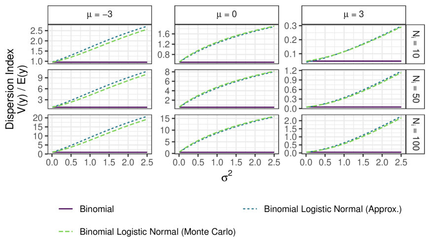
Fig. A1: Approximated BiL dispersion index versus Binomial dispersion index.

A2 Interpretation of $\sigma$ for BeC models

The use of the latent variable representation of the BeC models is helpful in getting a better understanding of what this model class represents. Below we focus on link functions that are cdf’s of scale mixtures of normals (which is the case for the most popular choices).

If we take for $Q(\cdot)$ the cdf of a standard Normal, the BeC model is equivalent to the Probit model with an extra unidentified parameter $\sigma^{2}$.

Choosing alternative $Q(\cdot)$ specifications maps out a class of models with a link function that sits in between that of the corresponding standard binary regression model and that of the Probit BeC model. For example, taking $Q(\cdot)$ to be a student-$t$ cdf with $\sigma^{2}=0$ leads to the ”$t$-link” model of Albert and Chib (1993). Let us consider the latent variable representation of this model as follows: $y_{i}=1$ for some latent variable $w_{i}>0$ and $y_{i}=0$ for $w_{i}\leq 0$ with $w_{i}\sim N(\alpha+\bm{x}_{i}^{\prime}\bm{\beta},\lambda_{i}^{-1})$, where $\lambda_{i}\sim\mathcal{G}(\nu/2,\nu/2)$. Extending this to the ULLGM setting gives us $w_{i}|z_{i}\sim N(z_{i},\lambda_{i}^{-1})$, and integrating out $z_{i}$ with (2) leads to $w_{i}\sim N(\alpha+\bm{x}_{i}^{\prime}\bm{\beta},\sigma^{2}+\lambda_{i}^{-1})$. Thus, the probability that $y_{i}=1$ becomes

$$P(y_{i}=1)=\mathbb{E}_{\lambda_{i}}\left\{\Phi\left(\frac{\alpha+\bm{x}_{i}^{\prime}\bm{\beta}}{\sqrt{\sigma^{2}+\lambda_{i}^{-1}}}\right)\right\},$$ (A9)

where $\Phi(\cdot)$ denotes the cdf of the standard Normal distribution. Clearly, if $\sigma^{2}=0$ this simply describes the $t$-link model and as $\sigma^{2}\to\infty$ we will tend to the overparameterised Probit model with $P(y_{i}=1)=\Phi(\{\alpha+\bm{x}_{i}^{\prime}\bm{\beta}\}/\sigma)$. For nonzero finite values of $\sigma^{2}$, the probability in (A9) together with $\lambda_{i}\sim\mathcal{G}(\nu/2,\nu/2)$ describes a hybrid model. That is, in BeC models, the interpretation of $\sigma^{2}$ is the relative weight of the Probit link version. If we take $Q(\cdot)$ to be the logistic cdf instead, the same kind of argument holds, only changing the distribution for $\lambda_{i}$. In particular, (A9) applies where now $\lambda_{i}=(2\psi_{i})^{2}$ and $\psi_{i}$ has a Kolmogorov-Smirnov distribution (Holmes and Held, 2006). An example for a Cauchy link is shown in Fig. A2. To scale things comparably for different values of $\sigma$, the figure plots simulated values of

$$P(y_{i}=1)=\mathbb{E}_{\lambda_{i}}\left\{\Phi\left(\frac{(\alpha+\bm{x}_{i}^{\prime}\bm{\beta})\sqrt{\sigma^{2}+1}}{\sqrt{\sigma^{2}+\lambda_{i}^{-1}}}\right)\right\},$$

for $\nu=1$ and values of $\sigma^{2}$ ranging from 0 (Cauchy link) to 250 (close to Probit link).

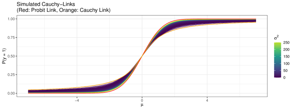
Fig. A2: Simulated link functions. Value of $\sigma^{2}$ determines proximity to probit link and Cauchy link.

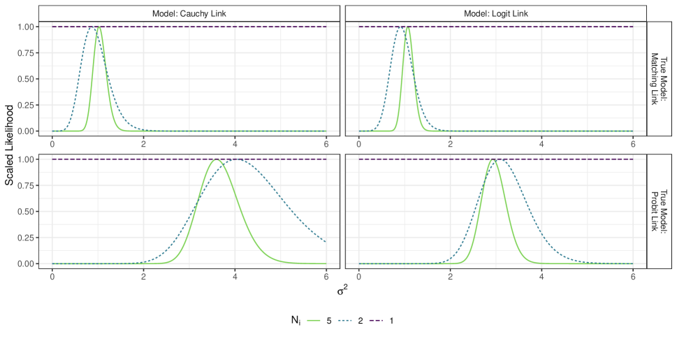
Fig. A3: Likelihood evaluations for different values of $\sigma^{2}$ and $N_{i}$ under Binomial ULLGM likelihood under a logistic link function (right column) and a Cauchy link function (left column). Data generating processes follow either a misspecified probit model (bottom row) or the correct Logit or Cauchy link function (top row). In all simulated data sets, $\sigma^{2}=1$ and $n=1,000$.

Fig. A3 illustrates the likelihood behavior of Binomial ULLGM models for various values of $\sigma^{2}$ and number of trials $N_{i}$ and for different specifications of $h(z)$, using logistic and Cauchy link functions. The data are generated from Binomial ULLGMs with $\sigma^{2}=1$ and three possible link functions: the Cauchy or logistic link functions lead to correct model specifications and the probit link function leads to misspecification. The figure highlights that while $N_{i}>1$ provides likelihood information about $\sigma^{2}$, the likelihood for the Bernoulli case, where $N_{i}=1$, is completely flat with respect to $\sigma^{2}$. This implies that $\sigma^{2}$ cannot be identified from the likelihood for BeC models. Consequently, the posterior distribution becomes improper under the prior in (8)-(9), as discussed in Sec. A5. Inference on $\sigma^{2}$ will be fully determined by the prior on $\sigma^{2}$, which needs to be proper.

A3 Effect of Neglecting Overdispersion in Poisson and Binomial Regression

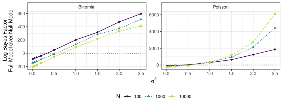
Fig. A4: Log Bayes factors of full model over null model for Binomial and Poisson regression for various overdispersion parameters $\sigma^{2}$. Refer to the text for details.

To illustrate the shortcomings of neglecting overdispersion in model averaging for non-Gaussian models, we conduct a small simulation exercise. Data were simulated from both a BiL model (with 100 trials per observation) and a PLN model, with overdispersion parameter $\sigma^{2}$ ranging from 0.01 (approximating the GLM case) to 2.5 (indicating clear overdispersion). We vary the sample sizes ($n\in\{100,1000,10000\}$) while keeping the number of iid standard Gaussian regressors constant at $p=50$. The linear predictor $z_{i}$ is simulated from $\mathcal{N}(2,\sigma^{2})$, implying no relationship with the regressors. We analysed these data with Poisson and Binomial models and approximated the log Bayes factors of the full model over the null model using the BIC approximation $0.5\times(\text{BIC}_{\text{Null}}-\text{BIC}_{\text{Full}})$. Each setting was replicated 100 times, and the median Bayes factors across these replications are displayed in Figure A4.

The results demonstrate that with increasing overdispersion, models without additional variation mechanisms attempt to account for the data variation by adding extra covariates and increasingly favoring larger models. This effect is more pronounced in the Poisson case, which has a more rigid variance structure compared to the binomial case, where variance is influenced by both the number of trials, and the imbalance of the dataset (as reflected in the success probabilities). Nonetheless, in both cases, even moderate amounts of overdispersion strongly favor the full model over the correct null model, even with sample size $n$ growing large. Interestingly, for the Poisson model this effect gets stronger with $n$, while for the Binomial it goes the other way.

A4 Uncertainty in $z_{i}$, MCMC efficiency and limiting cases of PLN and BiL models

To develop an understanding of the spread or concentration of the posterior distribution of $z_{i}$ in the PLN and BiL models, it is helpful to examine the posterior approximations derived in Sec. A11. For the PLN model, the posterior distribution is approximated as follows:

$$\begin{split}z_{i}&\sim\mathcal{N}\left(m,s\right)\\ s&=\left(y_{i}+\sigma^{-2}\right)^{-1}\\ m&=s\left(\log(y_{i})y_{i}+(\alpha+\bm{x}^{\prime}_{i}\bm{\beta})\sigma^{-2}\right),\end{split}$$ (A10)

From this, it becomes evident that larger $y_{i}$ imply a smaller posterior variance. As $y_{i}\rightarrow\infty$, the posterior distribution of $z_{i}$ converges to a point mass at $\log(y_{i})$. Conversely, smaller values of $y_{i}$ result in greater uncertainty in the likelihood contributions of observation $i$. For observations where $y_{i}=0$, the Poisson likelihood contribution $\mathcal{P}(e^{z_{i}})$ provides minimal information beyond $z_{i}<2$, and in fact the likelihood function degenerates. Consequently, a certain number of non-zero outcomes is necessary for a proper posterior under improper priors (compare the corresponding proof conditions in Sec. A5). This indicates that likelihood identification of $z_{i}$, and therefore MCMC efficiency, strongly depends on the number of zero outcomes and the size of the remaining counts. For very large counts, the PLN model behaves approximately like a Gaussian regression model with outcome $\log(y_{i})$. For small counts, $z_{i}$ is more strongly informed by prior information, resulting in decreased MCMC efficiency due to increased dependency between $z_{i}$ and $\alpha$, $\bm{\beta}$, and $\sigma^{2}$.

Similar considerations apply to the BiL framework, where the posterior approximation of $z_{i}$ from Sec. A11 is given by:

$$\begin{split}z_{i}&\sim\mathcal{N}\left(m,s\right)\\ s&=\left([\hat{p}_{i}(1-\hat{p}_{i})N_{i}]+\sigma^{-2}\right)^{-1}\\ m&=s\left([\text{logit}(\hat{p}_{i}){N_{i}\hat{p}_{i}(1-\hat{p}_{i})}]+(\alpha+\bm{x}^{\prime}_{i}\bm{\beta})\sigma^{-2}\right).\end{split}$$ (A11)

From this approximation, it can be seen that likelihood identification is strongest when $N_{i}\gg 1$ and $y_{i}\approx 0.5N_{i}$. For such observations, the BiL model behaves approximately like a Gaussian regression model with outcome $\text{logit}(y_{i}/N_{i})$ as $z_{i}\rightarrow\text{logit}(y_{i}/N_{i})$ when $N_{i}\rightarrow\infty$, with the approximation becoming accurate faster when $\hat{p}_{i}\approx 0.5$. Conversely, as $N_{i}$ approaches a single trial (Bernoulli case) and/or outcomes become more imbalanced ($y_{i}$ close to 0 or $N_{i}$), likelihood identification weakens and MCMC efficiency decreases. When $y_{i}=0$ or $y_{i}=N_{i}$, the likelihood contributions become degenerate, even for large $N_{i}$, which is reflected in the conditions for the proofs in Sec. A5.

A5 Proof of Theorem 1

In this Appendix, we will derive the conditions under which the posterior resulting from the sampling model in (1) and (6) is well-defined under the improper prior structure in (8) and (9) for any model in the model space. Theorem 1 considers the case where any additional parameter $r$ is fixed. Thus, in the proof we will not explicitly condition on $r$.

Denote by $\bm{y}$ the vector of all observations $y_{i}$ and partition $\bm{y}$ as $\bm{y}=(\bm{y}_{N}^{\prime},\bm{y}_{Z}^{\prime})^{\prime}$ where $\bm{y}_{N}$ groups all $n_{N}$ observations that allow for the integral $\int P(y_{i}|z_{i})dz_{i}$ to be finite. Now consider the marginal likelihood for model $M_{k}$

$$P(\bm{y}|M_{k})=P(\bm{y}_{Z}|\bm{y}_{N},M_{k})P(\bm{y}_{N}|M_{k})$$ (A12)

and we need to show that this marginal likelihood is finite for all values of $\bm{y}$ and for any model $M_{k}$. First, let us focus on the vector $\bm{y}_{N}$:

$$P(\bm{y}_{N}|M_{k})=\int P(\bm{y}_{N}|\bm{z}_{N},M_{k})p(\bm{z}_{N}|M_{k})d\bm{z}_{N},$$ (A13)

where $\bm{z}_{N}$ denotes those $z_{i}$ that correspond to $\bm{y}_{N}$ and we can write

$$P(\bm{y}_{N}|\bm{z}_{N},M_{k})=\prod_{i\in\cal N}P({y}_{i}|{z}_{i}),$$ (A14)

where $\cal N$ is the set of observation indices of $\bm{y}_{N}$. Let us now consider $p(\bm{z}_{N}|M_{k})$. If the matrix $(\iota:\bm{X_{k}})$ is of full column rank (Condition 1) and if $n_{N}\geq 2$ (Condition 2), we can derive that

$$p(\bm{z}_{N}|M_{k})\propto g^{-\frac{p_{k}}{2}}|\bm{X}_{k}^{\prime}\bm{X}_{k}|^{\frac{1}{2}}|\bm{A}_{k}|^{-\frac{1}{2}}[\bm{z}_{N}^{\prime}\bm{P}_{k}\bm{z}_{N}]^{-\frac{n_{N}-1}{2}},$$ (A15)

where

$$\bm{P}_{k}=I_{n_{N}}-(\iota:\bm{X}_{k,N})\left({\begin{array}[]{cc}n_{N}^{-1}&\bm{0}^{\prime}\\ \bm{0}&\bm{A}_{k}^{-1}\\ \end{array}}\right)\left(\begin{array}[]{c}\iota^{\prime}\\ \bm{X}_{k,N}^{\prime}\\ \end{array}\right)$$ (A16)

and $\bm{A}_{k}=\bm{X}_{k,N}^{\prime}\bm{X}_{k,N}+g^{-1}\bm{X}_{k}^{\prime}\bm{X}_{k}$. Under Condition 1, $\bm{A}_{k}$ is invertible and for fixed choices of $g$, the expression in (A15) is almost surely bounded from above by a finite number, say $c$. For hyperpriors on $g$ that are proper distributions with pdf $p(g)$, the relevant marginal likelihood for $\bm{z}_{N}$ is the expression in (A15) integrated with respect to $p(g)$. As $g$ tends to zero, (A15) tends to a finite constant in $g$ and as $g$ tends to $\infty$ the expression in (A15) behaves like $g^{-p_{k}/2}$. Thus any proper $p(g)$ will lead to a finite value of the marginal likelihood $p(\bm{z}_{N}|{M}_{k})$. For the null model $M_{0}$ with only the intercept, the prior is simply (8) and the marginal likelihood is

$$p(\bm{z}_{N}|{M}_{0})\propto[(\bm{z}_{N}-\bar{z}_{N}\iota)^{\prime}(\bm{z}_{N}-\bar{z}_{N}\iota)]^{-\frac{n_{N}-1}{2}}$$ (A17)

(with the same proportionality constant as in (A15)), which is also bounded. In the latter expression we have defined

$$\bar{z}_{N}=\frac{1}{n_{N}}\sum_{i\in\cal N}z_{i}.$$ (A18)

Therefore, (A13) becomes

$$P(\bm{y}_{N}|M_{k})<c\prod_{i\in\cal N}\int P({y}_{i}|{z}_{i})d{z}_{i},$$ (A19)

and it is sufficient to show that each of the integrals in the above expression is finite. In the sequel, we will consider the models presented in Table 1 and drop subscripts for convenience.

A5.1 PLN model

Here, we consider

$$I=\int_{\Re}P({y}|{z})d{z}=\int_{\Re}\frac{\exp[-\exp(z)](\exp{z})^{y}}{y!}dz,$$ (A20)

and use the variable transformation $h=\exp(z)$ to obtain

$$I=\frac{1}{y!}\int_{\Re_{+}}\exp[-h]h^{y-1}dh=\frac{1}{y!}\Gamma(y)=\frac{1}{y},$$ (A21)

which means that $\bm{y}_{N}$ consists of all nonzero observations. This leads directly to

$$P(\bm{y}_{N}|M_{k})<c\prod_{i\in\cal N}\frac{1}{y_{i}}<\infty.$$ (A22)

Thus, we have a well-defined posterior distribution after taking into account at least 2 nonzero observations. These observations in $\bm{y}_{N}$ will then update the improper prior into a proper posterior which can then be used as the (proper) prior for the analysis of the zero observations in $\bm{y}_{Z}$. Of course, the latter will lead to a proper posterior with a finite integrating constant. Thus, $P(\bm{y}_{Z}|\bm{y}_{N},M_{k})<\infty$ and using (A12) and (A22) we obtain that $P(\bm{y}|M_{k})<\infty$ which proves the result. Conditions 1 and 2 jointly are thus sufficient for propriety. Condition 1 is also necessary, since we need $\bm{X}_{k}$ to be of full column rank for the prior specification in (9) and given that the regressors are demeaned this also implies that Condition 1 holds. In order to prove that Condition 2 is also necessary for propriety, we consider the same line of proof as in Subsection A5.7. If condition 2 does not hold, we need to rely on observations for which $y_{i}=0$ to obtain a proper posterior ($\bm{y}_{N}$ with $n_{N}<2$ does not lead to a proper posterior). As explained in Subsection A5.7, the integral in (A38) then needs to integrate in each $z_{i}$ which requires that $P(y_{i}|z_{i},M_{k})$ tends to zero in the tails for $z_{i}$. For $y_{i}=0$ we have

$$P(y_{i}=0|z_{i},M_{k})=\exp[-\exp(z_{i})],$$ (A23)

which tends to 1 as $z_{i}\to-\infty$. Thus, (A38) will not integrate and condition 2 is necessary for posterior propriety in the PLN model.

If we change the distribution for the observables $y_{i}$ or the link function $h(\cdot)$, then all that changes in the proof is the definition of $\bm{y}_{N}$ and the expression for (A19).

A5.2 NBL model

If $y\sim$ Negative Binomial$\left(r,\frac{\exp(z)}{1+\exp{z}}\right)$ then the integrals in (A19) are

$$I=\int_{\Re}P({y}|{z})d{z}={r+y-1\choose y}\int_{\Re}\pi^{r}(1-\pi)^{y}dz,$$ (A24)

defining $\pi=\frac{\exp(z)}{1+\exp{z}}$. Thus, we obtain

$$I={r+y-1\choose y}\int_{0}^{1}\pi^{r}(1-\pi)^{y}\left|\frac{d\pi}{dz}\right|^{-1}d\pi={r+y-1\choose y}\int_{0}^{1}\pi^{r-1}(1-\pi)^{y-1}d\pi=\frac{1}{y}.$$ (A25)

The integral above is finite for all observations where $y>0$. Thus, if we denote by $\bm{y}_{N}$ those observations for which $y_{i}>0$, we have

$$P(\bm{y}_{N}|M_{k})<c<\infty,$$ (A26)

which means that we have a well-defined posterior distribution after taking into account at least 2 observations in $\bm{y}_{N}$. The rest of the proof mirrors that for the PLN model. If we do not have two observations for which $y_{i}>0$, we can use the same arguments as in Subsection A5.7 to show that the posterior does not exist, so that conditions 1 and 2 are both necessary and sufficient for posterior propriety in the NBL case.

A5.3 BiL model

If we use Binomial $y\sim Bin\left(N,\frac{\exp(z)}{1+\exp{z}}\right)$ then we obtain

$$I=\int_{\Re}P({y}|{z})d{z}={N\choose y}\int_{\Re}\pi^{y}(1-\pi)^{N-y}dz,$$ (A27)

defining $\pi=\frac{\exp(z)}{1+\exp{z}}$. Thus, we obtain

$$I={N\choose y}\int_{0}^{1}\pi^{y}(1-\pi)^{N-y}\left|\frac{d\pi}{dz}\right|^{-1}d\pi={N\choose y}\int_{0}^{1}\pi^{y-1}(1-\pi)^{N-y-1}d\pi.$$ (A28)

The integrand above is the kernel of a Beta$(y,N-y)$ distribution. Provided we have $0<y<N$, this leads to

$$I={N\choose y}\frac{\Gamma(y)\Gamma(N-y)}{\Gamma(N)}=\frac{N}{y(N-y)}$$ (A29)

The latter expression is finite for all observations where $0<y<N$. Thus, if we denote by $\bm{y}_{N}$ those observations for which $0<y_{i}<N_{i}$, we have

$$P(\bm{y}_{N}|M_{k})<c\prod_{i}\frac{N_{i}}{y_{i}(N_{i}-y_{i})}<\infty,$$ (A30)

which means that we have a well-defined posterior distribution after taking into account at least 2 observations in $\bm{y}_{N}$. The rest of the proof mirrors that for the PLN model. If we do not have two observations for which $0<y_{i}<N_{i}$, we can use the same arguments as in Subsection A5.7 to show that the posterior does not exist, so that conditions 1 and 2 are both necessary and sufficient for posterior propriety in the case of the BiL model.

A5.4 ErLN models

The Erlang case where $y_{i}\sim$ Erlang$(r,\lambda)$ (i.e. a Gamma distribution with integer shape parameter $r=1,2,\dots$) covers the Exponential model if we take $r=1$. We assume that $\lambda=\exp(z)$, so that the integrals in (A19) are given by

$$I=\int_{\Re_{+}}p({y}|{z})d{z}=\frac{y^{r-1}}{\Gamma(r)}\int_{\Re_{+}}\exp(rz)\exp\{-y\exp(z)\}dz.$$ (A31)

Using the transformation $\lambda={\exp(z)}$, we obtain

$$I=\frac{y^{r-1}}{\Gamma(r)}\int_{\Re_{+}}\lambda^{r-1}\exp\{-y\lambda\}d\lambda=\frac{1}{y}.$$ (A32)

This integral is finite for all observations where $y$ is different from 0. This is an event of measure zero in the sampling distribution, so the posterior distribution is almost surely well-defined for any value of $r$, taking $\bm{y}_{N}=\bm{y}$.

A5.5 LNN model

If we use log Normal sampling $y_{i}\sim$ log-Normal$(\mu,1)$ with $\mu=z$, the integrals in (A19) are given by

$$I=\int_{\Re}p({y}|{z})d{z}={\frac{1}{y\sqrt{2\pi}}}\int_{\Re}\exp{-\frac{1}{2}{(\ln y-\mu)^{2}}}d\mu.$$ (A33)

This immediately leads to

$$I={\frac{1}{y}},$$ (A34)

which is finite for all observations where $y>0$. The event $y=0$ has zero probability in the sampling distribution, so the posterior distribution is almost surely well-defined, taking $\bm{y}_{N}=\bm{y}$.

A5.6 LNLN model

If we use log Normal sampling $y_{i}\sim$ log-Normal$(r,\lambda)$ with $\lambda=\exp(z)$, the integrals in (A19) are given by

$$I=\int_{\Re}p({y}|{z})d{z}={\frac{1}{y\sqrt{2\pi}}}\int_{\Re}\lambda^{-\frac{1}{2}}\exp{-\frac{(\ln y-r)^{2}}{2\lambda}}dz.$$ (A35)

Using the transformation $\lambda={\exp(z)}$, we obtain

$$I={\frac{1}{y\sqrt{2\pi}}}\int_{\Re_{+}}\lambda^{-\frac{3}{2}}\exp{-\frac{(\ln y-r)^{2}}{2\lambda}}d\lambda,$$ (A36)

which can be solved using the inverse gamma distribution to leave us with

$$I=\frac{1}{y|\ln y-r|}.$$ (A37)

This integral is finite for all observations where $y$ is different from 0 or $\exp(r)$. These are events of measure zero in the sampling distribution, so the posterior distribution is almost surely well-defined, taking $\bm{y}_{N}=\bm{y}$.

A5.7 Bernoulli-based models BeC

Consider the marginal likelihood for model $M_{k}$ based on the entire sample:

$$P(\bm{y}|M_{k})=\int P(\bm{y}|\bm{z},M_{k})p(\bm{z}|M_{k})d\bm{z}=\int\prod_{i=1}^{n}P({y_{i}}|z_{i},M_{k})p(\bm{z}|M_{k})d\bm{z}.$$ (A38)

As explained in Appendix A5.8, the marginal density of $\bm{z}$ given $M_{k}$ is a quadratic form which does not have sufficiently thin tails to integrate in $\bm{z}$. Thus, for the integral in (A38) to be finite the tails need to be squeezed by $\prod_{i}P({y_{i}}|z_{i},M_{k})$. In other words, when integrating with respect to $z_{i}$, the corresponding $P({y_{i}}|z_{i},M_{k})$ needs to go to zero fast enough as $z_{i}$ tends to $\infty$ and $-\infty$. Since

$$P({y_{i}}|z_{i},M_{k})=\pi_{i}^{y_{i}}(1-\pi_{i})^{1-y_{i}}$$ (A39)

and we have a link function in BeC models that associates $z_{i}\to\infty$ with $\pi_{i}\to 1$ it is clear that an observed $y_{i}=1$ will not change the right-hand tail of $p(\bm{z}|M_{k})$ along dimension $i$ ( $P(y_{i}=1|z_{i},M_{k})=\pi_{i}$, which will be bounded from below for large $z_{i}$). Similarly, the value $y_{i}=0$ will leave the left-hand tail untouched. Thus, for any possible observation the marginal likelihood in (A38) will not be finite and the posterior will not exist.

A5.8 Marginal prior distribution of $z$

As stated in (14), the marginal likelihood under fixed $g$ is

$$p(\bm{z}|M_{k})\propto(1+g)^{\frac{n-1-p_{k}}{2}}\left[\{1+g(1-R_{k}^{2})\}(\bm{z}-{\bar{z}}\iota)^{\prime}(\bm{z}-{\bar{z}}\iota)\right]^{-\frac{n-1}{2}},$$ (A40)

where $R_{k}^{2}$ is the coefficient of determination of $\bm{z}$ regressed on $\bm{X}_{k}$ (and an intercept). Thus, the pdf of $\bm{z}$ can be written as

$$p(\bm{z}|M_{k}) \propto\left[g\bm{z}^{\prime}Q_{\bm{W}_{k}}\bm{z}+(\bm{z}-{\bar{z}}^{\prime}\iota)^{\prime}(\bm{z}-{\bar{z}}^{\prime}\iota)\right]^{-\frac{n-1}{2}}$$ (A41)

$$=\left[g\bm{z}^{\prime}Q_{\bm{W}_{k}}\bm{z}+\bm{z}^{\prime}(I-\frac{1}{n}\iota\iota^{\prime})\bm{z}\right]^{-\frac{n-1}{2}}$$ (A42)

$$=\left[\bm{z}^{\prime}{\bm{V}}_{k}\bm{z}\right]^{-\frac{n-1}{2}},$$ (A43)

where we have defined $\bm{W}_{k}=(\iota:\bm{X}_{k})$ and

$$\bm{V}_{k}=(1+g)I-\frac{1}{n}\iota\iota^{\prime}-g\bm{W}_{k}(\bm{W}_{k}^{\prime}\bm{W}_{k})^{-1}\bm{W}_{k}^{\prime},$$ (A44)

The $n\times n$ matrix $\bm{V}_{k}$ is positive definite as it is the sum of two positive definite matrices. The distribution of $\bm{z}$ for each model is reminiscent of a multivariate Student-$t$ but is not a proper distribution as it would correspond to negative degrees of freedom and an unbounded density at zero. As expected, the expression for $p(\bm{z}_{N}|M_{k})$ in (A15) simplifies to (A43) if we take $\bm{z}_{N}=\bm{z}$, barring a proportionality constant $(1+g)^{\frac{n-1-p_{k}}{2}}$, which appears in (A40) but is immaterial to the considerations in this section.

A6 Proof of Theorem 2

This theorem applies to models with additional parameters and its proof has a similar structure as that for Theorem 1.

Again, we focus on the marginal likelihood for a subsample $\bm{y}_{N}$ which groups the observations corresponding to a finite $\int P(y_{i}|z_{i},r)dz_{i}$. We can write for the marginal likelihood of $\bm{y}_{N}$ in model $M_{k}$:

$$P(\bm{y}_{N}|M_{k})=\int P(\bm{y}_{N}|\bm{z}_{N},r,M_{k})p(\bm{z}_{N}|M_{k})P(r|\bm{z}_{N},M_{k})d\bm{z}_{N}dr.$$ (A45)

Using the fact that $p(\bm{z}_{N}|M_{k})$ is bounded by some finite constant $c$ under conditions 1 and 2 (see the proof of Theorem 1), and applying (7) along with (A14), we obtain

$$P(\bm{y}_{N}|M_{k})<c\int P(\bm{y}_{N}|\bm{z}_{N},r,M_{k})P(r|M_{k})d\bm{z}_{N}dr=c\int\prod_{i\in\cal N}P({y}_{i}|{z}_{i},r)d{z}_{i}P(r|M_{k})dr.$$

Substituting the definition of $f(r)$ in (17), we obtain directly

$$P(\bm{y}_{N}|M_{k})<c\int f(r)P(r|M_{k})dr,$$ (A46)

so that the condition in (16) is sufficient for posterior existence. The rest of the proof follows a similar reasoning to the proof of Theorem 1.

For the LNLN model we have

$$f(r)=\prod_{i=1}^{n}\frac{1}{y_{i}|\ln y_{i}-r|}$$

from (A37), which means that the condition in (16) would require the prior on $r$ to compensate for $f(r)$ behaving like $1/|r|$ in $n$ neighbourhoods around $\ln(y_{i})$. This would need the prior on $r$ to have vanishing mass in these neighbourhoods, but of course their location depends on the observations. Thus, there is no (non-data based) prior that can satisfy (16) for the LNLN model, so we can not conclude that posterior inference on $r$ can be conducted with the overall prior structure assumed here for the LNLN model.

A7 Log Posterior Gradients for PLN and BiL models

Note that in any ULLGM model, the gradient of the conditional log posterior of $z_{i}$ additively decomposes into two parts. The first part is the gradient of the log of the Gaussian prior $p(z_{i}|\alpha,\bm{\beta},\sigma^{2},\bm{x}_{i})$. Regardless of which likelihood is chosen as the basis for a ULLGM, this gradient is given by

$$\frac{\partial\log p(z_{i}|\alpha,\bm{\beta},\sigma^{2},\bm{x}_{i})}{\partial z_{i}}=-\frac{z_{i}-\alpha-\bm{x}_{i}\bm{\beta}}{\sigma^{2}}.$$

The second part is the gradient of the log of the likelihood term $P(y_{i}|h(z_{i}),r)$, which depends on the type of model. For the PLN model, we have that

$$P(y_{i}|z_{i})=\frac{e^{y_{i}z_{i}}e^{-e^{z_{i}}}}{y_{i}!}$$

and hence

$$\frac{\partial\log P(y_{i}|z_{i})}{\partial z_{i}}=y_{i}-e^{z_{i}}.$$

For the BiL model, we have that

$$P(y_{i}|z_{i},N_{i})=\left(N_{i}\atop y_{i}\right)p_{i}^{y_{i}}(1-p_{i})^{N_{i}-y_{i}}$$

and hence

$$\frac{\partial\log P(y_{i}|z_{i})}{\partial z_{i}}=\frac{y_{i}-(N_{i}-y_{i})e^{z_{i}}}{1+e^{z_{i}}}.$$

A8 Details on Add-Delete-Swap Proposal

In the context of proposing a new candidate model $M^{*}$, our approach involves deciding between three potential moves—addition, swap, and deletion—to transition between models. Let $p$ denote the total number of predictors, and let $p_{k}$ denote the number of predictors currently included in the model. The move is selected based on the current composition of the model:

• If $p_{k}=0$, the only possible move is addition.

• If $p_{k}=p$, the only possible move is deletion.

• Otherwise, any of the three moves may be chosen, with the choice made uniformly at random.

This setup requires accounting for appropriate correction terms in the Metropolis-Hastings acceptance probability to ensure detailed balance. We denote the probability of proposing a move from the current model $M_{k}$ to a proposed model $M^{*}$ as $q(M^{*}\mid M_{k})$, and the reverse move probability as $q(M_{k}\mid M^{*})$.

• Addition:

  $$q(M^{*}\mid M_{k})=\left(\frac{1}{p-p_{k}}\right)$$

  $$q(M_{k}\mid M^{*})=\left(\frac{1}{p^{*}}\right).$$

  Here, $p^{*}=p_{k}+1$ is the number of predictors after the addition. This reflects the uniform probability of selecting any of the $p^{*}$ predictors in $M^{*}$ for deletion to reverse to $M_{k}$.

• Swap: In this case, the proposal is symmetric and therefore

  $$\frac{q(M_{k}\mid M^{*})}{q(M^{*}\mid M_{k})}=1.$$

• Deletion:

  $$q(M^{*}\mid M_{k})=\left(\frac{1}{p_{k}}\right)$$

  $$q(M_{k}\mid M^{*})=\left(\frac{1}{p-p^{*}}\right).$$

  Here, $p^{*}=p_{k}-1$ is the number of predictors after the deletion. This reflects the uniform probability of selecting any of the $p-p^{*}$ predictors not in $M^{*}$ for addition to reverse to $M_{k}$.

A9 Results for Simulated Data

Prior	DGP	$n$	$p$	$\mathcal{M}$ Size	Frac. True	Brier	FNR	FPR	ln(g)	$\sigma^{2}$
Poisson Log-Normal
Hyper-g/n (a=3)	ULLGM	150	50	14.848	0.006	0.026	0.034	0.137	3.971	0.180
Hyper-g/n (a=3)	ULLGM	150	100	15.248	0.005	0.010	0.049	0.064	4.134	0.186
Hyper-g/n (a=3)	ULLGM	1000	50	14.894	0.010	0.021	0.012	0.128	3.940	0.197
Hyper-g/n (a=3)	ULLGM	1000	100	15.072	0.010	0.007	0.012	0.060	4.069	0.198
Hyper-g/n (a=3)	GLM	150	50	13.529	0.046	0.009	0.001	0.090	6.297	0.014
Hyper-g/n (a=3)	GLM	150	100	13.451	0.046	0.003	0.001	0.041	6.312	0.010
Hyper-g/n (a=3)	GLM	1000	50	13.562	0.025	0.012	0.001	0.095	8.022	0.002
Hyper-g/n (a=3)	GLM	1000	100	13.619	0.035	0.003	0.000	0.041	8.026	0.006
Hyper-g/n (a=3)	Log-Gamma	150	50	14.873	0.005	0.025	0.035	0.131	4.184	0.158
Hyper-g/n (a=3)	Log-Gamma	150	100	15.263	0.004	0.011	0.040	0.065	4.336	0.160
Hyper-g/n (a=3)	Log-Gamma	1000	50	14.707	0.010	0.021	0.015	0.121	4.105	0.169
Hyper-g/n (a=3)	Log-Gamma	1000	100	14.561	0.013	0.006	0.013	0.052	4.248	0.173
Unit Information (g=n)	ULLGM	150	50	12.907	0.014	0.020	0.044	0.086	5.011	0.146
Unit Information (g=n)	ULLGM	150	100	13.630	0.010	0.009	0.048	0.044	5.011	0.147
Unit Information (g=n)	ULLGM	1000	50	10.102	0.091	0.011	0.089	0.023	6.908	0.195
Unit Information (g=n)	ULLGM	1000	100	10.718	0.182	0.002	0.041	0.012	6.908	0.190
Unit Information (g=n)	GLM	150	50	13.905	0.033	0.011	0.001	0.098	5.011	0.043
Unit Information (g=n)	GLM	150	100	14.154	0.030	0.003	0.000	0.047	5.011	0.035
Unit Information (g=n)	GLM	1000	50	13.707	0.028	0.012	0.000	0.096	6.908	0.009
Unit Information (g=n)	GLM	1000	100	13.932	0.032	0.003	0.000	0.044	6.908	0.009
Unit Information (g=n)	Log-Gamma	150	50	13.321	0.017	0.018	0.036	0.092	5.011	0.142
Unit Information (g=n)	Log-Gamma	150	100	14.553	0.008	0.010	0.024	0.055	5.011	0.116
Unit Information (g=n)	Log-Gamma	1000	50	10.320	0.137	0.008	0.065	0.023	6.908	0.163
Unit Information (g=n)	Log-Gamma	1000	100	10.672	0.149	0.003	0.048	0.012	6.908	0.173
Binomial Logistic-Normal
Hyper-g/n (a=3)	ULLGM	150	50	14.907	0.003	0.029	0.047	0.136	4.053	0.181
Hyper-g/n (a=3)	ULLGM	150	100	15.301	0.003	0.012	0.062	0.067	4.201	0.177
Hyper-g/n (a=3)	ULLGM	1000	50	14.693	0.008	0.022	0.021	0.124	4.020	0.198
Hyper-g/n (a=3)	ULLGM	1000	100	15.285	0.007	0.009	0.017	0.064	4.064	0.194
Hyper-g/n (a=3)	GLM	150	50	13.886	0.032	0.011	0.001	0.099	6.369	0.018
Hyper-g/n (a=3)	GLM	150	100	14.048	0.032	0.004	0.001	0.046	6.216	0.022
Hyper-g/n (a=3)	GLM	1000	50	13.652	0.045	0.010	0.000	0.092	7.981	0.005
Hyper-g/n (a=3)	GLM	1000	100	13.751	0.040	0.003	0.000	0.042	8.184	0.004
Hyper-g/n (a=3)	Log-Gamma	150	50	14.942	0.003	0.029	0.050	0.145	3.959	0.210
Hyper-g/n (a=3)	Log-Gamma	150	100	15.602	0.002	0.012	0.044	0.068	4.165	0.185
Hyper-g/n (a=3)	Log-Gamma	1000	50	14.991	0.006	0.025	0.016	0.133	3.873	0.206
Hyper-g/n (a=3)	Log-Gamma	1000	100	15.015	0.008	0.009	0.020	0.060	4.020	0.211
Unit Information (g=n)	ULLGM	150	50	13.258	0.013	0.021	0.048	0.093	5.011	0.126
Unit Information (g=n)	ULLGM	150	100	14.427	0.005	0.012	0.035	0.053	5.011	0.116
Unit Information (g=n)	ULLGM	1000	50	10.271	0.118	0.009	0.077	0.023	6.908	0.188
Unit Information (g=n)	ULLGM	1000	100	10.537	0.113	0.004	0.057	0.012	6.908	0.193
Unit Information (g=n)	GLM	150	50	14.379	0.020	0.013	0.001	0.111	5.011	0.041
Unit Information (g=n)	GLM	150	100	14.404	0.024	0.003	0.001	0.050	5.011	0.045
Unit Information (g=n)	GLM	1000	50	13.840	0.033	0.011	0.000	0.096	6.908	0.008
Unit Information (g=n)	GLM	1000	100	14.117	0.030	0.003	0.000	0.046	6.908	0.009
Unit Information (g=n)	Log-Gamma	150	50	13.143	0.010	0.021	0.051	0.093	5.011	0.156
Unit Information (g=n)	Log-Gamma	150	100	14.288	0.012	0.009	0.038	0.051	5.011	0.138
Unit Information (g=n)	Log-Gamma	1000	50	10.177	0.098	0.010	0.085	0.021	6.908	0.207
Unit Information (g=n)	Log-Gamma	1000	100	10.543	0.147	0.003	0.053	0.012	6.908	0.205

• Note: ’DGP’ = data generating process; ’$\mathcal{M}$ size’ = expected model size; ’Frac. True’ = Fraction of MCMC iterations where true model is visited; ’Brier’ = Brier score; ’FNR’ = False negative rate; ’FPR’ = False positive rate. Results are averages across 100 replications per simulation setting.

Table A1: Results of Simulation Study.

Table A1 presents key statistics derived from the simulation outcomes, averaged across the replications. Posterior model size as well as the proportion of visits to the true model among all MCMC iterations are reported. In addition, we provide measures of the quality of the variable selection results. We consider the Brier score, which is a strictly proper scoring rule that corrects for the number of available covariates $p$. The Brier score is defined as $\frac{1}{p}\sum_{j=1}^{p}(\text{PIP}_{j}-a_{j})^{2}$. Here, $\text{PIP}_{j}$ is the posterior inclusion probability of covariate $j$ and $a_{j}=0$ if covariate $j$ is truly excluded while $a_{j}=1$ otherwise. The closer the Brier score is to zero, the more accurate the variable selection results are. In addition, the Table presents the average fractions of false positives and false negatives across all MCMC samples. Finally, we provide the fixed value or estimated posterior mean of $g$ on the log scale, as well as the posterior mean of $\sigma^{2}$.

A10 Bilateral Migration Flows Between OECD Countries

Quantitative models of human migration advance our understanding of migration behavior, can be used to improve existing migration estimates and to inform policy. Dyadic regression models are commonly used to analyze the spatial allocation of migrants, modeling migration flows based on the characteristics of the origin, destination, and the relationship between country pairs. Such models are extensively applied not just in migration studies but also to understand trade flows (Carrere, 2006) or tourism patterns (Morley et al., 2014). The preferred frequentist estimation method is the Pseudo Poisson maximum likelihood approach (Silva and Tenreyro, 2006), which simultaneously accounts for the count nature of the outcome data and potential overdispersion. Recent studies highlight a growing interest in applying probabilistic modeling to migration data (Bijak, 2010; Welch and Raftery, 2022), but the issue of model uncertainty has received limited attention in this field. Mitchell et al. (2011) explore migration to the UK using model averaging techniques, albeit within a Gaussian regression framework.

In this context, we use the PLN model to examine international migration flows among the 38 OECD countries from 2015 to 2020. These flows are estimates of Abel and Cohen (2019) following the methodology described in Azose and Raftery (2019), based on migrant stock data compiled by the United Nations. This challenging dataset comprises $n=38^{2}-38=1,406$ bilateral migration flows $y_{i}$, ranging from zero to over 1.6 million migrants (between Mexico and the United States). Dispersion in the data is very high, with the usual dispersion index over 345,000. The flows are depicted in the form of a circular plot in Supplementary Fig. A8. An initial analysis of the data highlights distinctive features of bilateral migration in this timeframe, such as the prominent migration corridor between Mexico and the United States and the central roles of Germany and the UK as migration hubs in Europe.

We have compiled a set of $p=54$ variables that hold potential predictive power for bilateral migration flows. This dataset encompasses a variety of country-specific factors for both origin and destination countries, including demographic measures like population size, population age distribution, and educational attainment rates, alongside economic indicators such as GDP per capita and employment rates. It also includes measures of social infrastructure, such as healthcare expenditure as a percentage of GDP, and indices of social and political stability, like the number of battle-related deaths, homicide rates, or the Gini coefficient measuring income inequality. These covariates collectively address a broad spectrum of theories that seek to explain international migration patterns, often highlighting the significance of labor market demands in destination countries, and the availability of knowledge, financial, and social capital in origin countries (De Haas et al., 2019). The dataset also features country-pair variables, like the distance between capitals, to acknowledge the tendency for increased migratory activity between geographically proximate countries. Furthermore, existing bilateral migration stocks and indicator variables for historical colonial ties or a common official language are included to capture the influence of non-geographical distance proxies such as existing migrant networks or cultural similarity on migration dynamics. More details, including summary statistics and the complete list of covariates are provided in Supplementary Table A6.

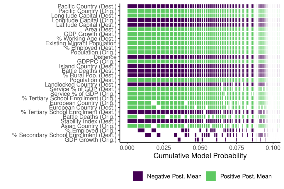
(a) Highest Probability Models.

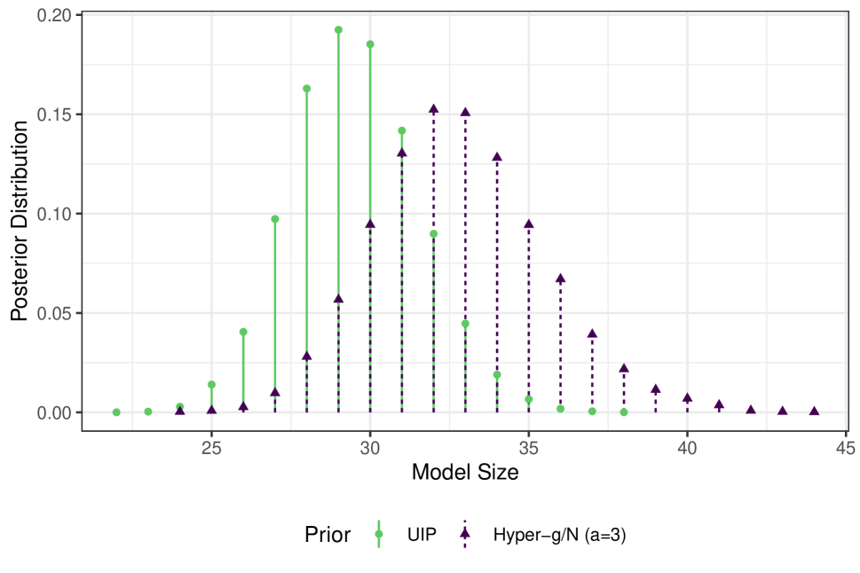
(b) Posterior Distribution of Model Size.

Fig. A5: Estimation Results (Bilateral Migration Flow Data). Highest probability models plot includes variables with estimated $\text{PIP}>0.3$ under unit information prior.

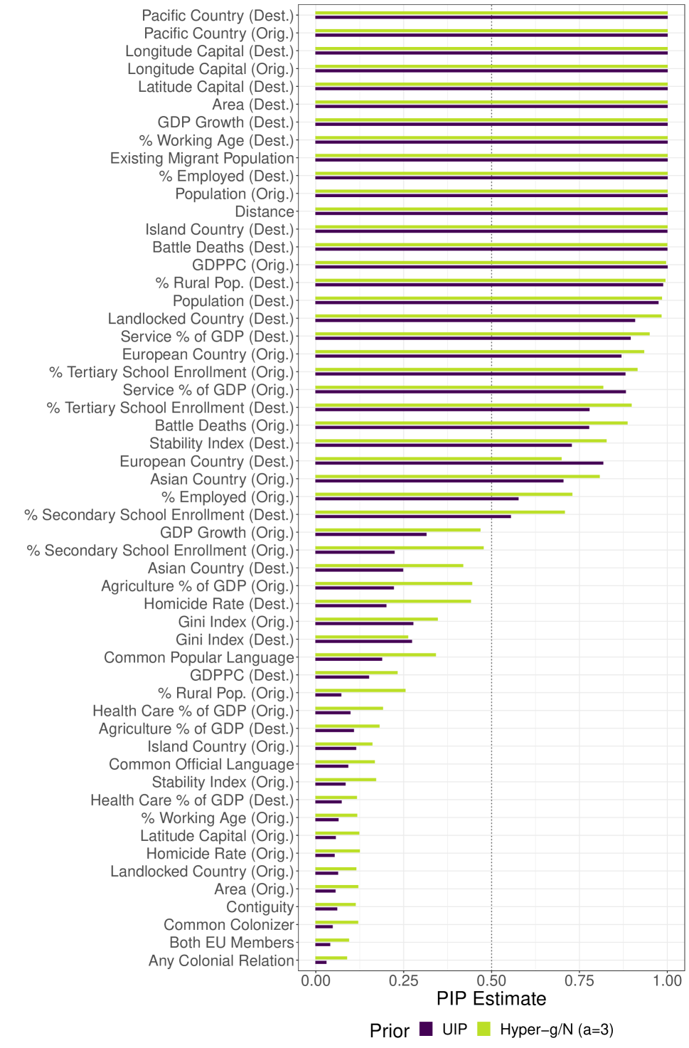
(a) Post. Inclusion Probabilities.

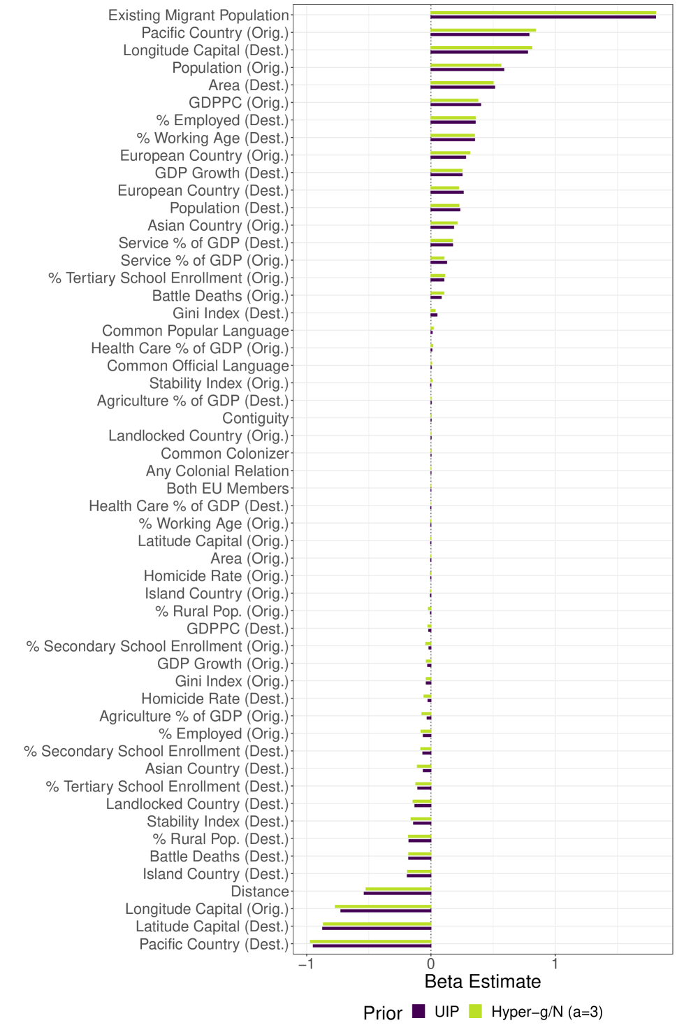
(b) Coefficient Post. Means.

Fig. A9: Estimation Results for Bilateral Migration Flow Data.

Based on this data, we conduct a BMA exercise using a Poisson Log-Normal specification. We compare a UIP prior ($g=n$) and a hyper-$g/n$ prior ($a=3$), alongside an agnostic prior on model space ($m=p/2$). The analysis is based on $300,000$ posterior samples after a burn-in period of $250,000$ iterations. The estimated posterior inclusion probabilities and the posterior means of $\bm{\beta}$ are presented in Supplementary Fig. A9. Under both priors, the posterior mean estimates for the intercept and the overdispersion parameter are $\mathbb{E}({\alpha}|\bm{y})=6.9$ and $\mathbb{E}({\sigma}^{2}|\bm{y})=0.7$, the latter indicating the presence of significant overdispersion in the model. The highest probability models under the unit information prior are shown in Fig. A5(a). The posterior model size distribution is depicted in Fig. A5(b), where the hyper-$g/n$ prior tends to support slightly larger models, with a posterior mean model size of $32.8$, compared to $29.5$ under the unit information prior.

The median probability models under the two priors (including those variables with a PIP estimate greater than 0.5) agree on a set of 29 covariates. The selected variables align with theoretical expectations about migration determinants, highlighting factors like distance (which is negatively correlated to migration flows), or the presence of existing bilateral migrant stocks (positive effect). Combined with the positive effects of population sizes, these findings underscore the roles of both mechanical factors and social networks in predicting migration flows. Additionally, the positive correlation between employment rates in destination countries and migration flows emphasizes the significance of labor markets and economic opportunity for international migration. Positive coefficients of indicator variables for Pacific countries reflect the high migration rates observed between Australia and New Zealand. Posterior model probabilities are relatively spread out, as detailed in Supplementary Table A8 and Table A9. Comprehensive details of the posterior means, standard deviations, and inclusion probabilities under both priors are available in Supplementary Table A7.

A11 Evaluation of Predictive Mass Function for PLN and BiL Models

To evaluate the quality of predictions in Sec. 7.3, we use LPS which require evaluations of the predictive pmf $P(y^{\text{p}}_{i}~{}|~{}\bm{x}^{\text{p}}_{i},\bm{y}^{\text{t}})$ in (18). In general, for the ULLGMs defined via (1) and (6), the likelihood contribution of a single data point $P(y_{i}|\bm{x}_{i},\alpha,\bm{\beta},\sigma^{2},M_{k})$ is given by

$$p(y_{i}|\bm{x}_{i},\bm{\theta},M_{k})=\int_{-\infty}^{\infty}F(y_{i}|h(z_{i}))~{}\mathcal{N}(z_{i}|\alpha+\bm{x}^{\prime}_{i,k}\bm{\beta}_{k},\sigma^{2})dz_{i},$$ (A47)

where $\bm{x}_{i,k}^{\prime}$ is the $i$th row of $\bm{X}_{k}$ and $\bm{\theta}=(\alpha,\bm{\beta},\sigma^{2})\in\Theta$. Under the PLN model, this becomes

$$\begin{split}P(y_{i}|&\bm{x}_{i},\bm{\theta},M_{k})=\\ &(2\pi\sigma^{2})^{-\frac{1}{2}}\int_{0}^{\infty}\exp(-\lambda_{i})\frac{\lambda_{i}^{y_{i}-1}}{y_{i}!}\exp\left(-\frac{1}{2\sigma^{2}}(\log\lambda_{i}-\alpha-\bm{x}^{\prime}_{i,k}\bm{\beta}_{k})^{2}\right)d\lambda_{i}.\end{split}$$ (A48)

Similarly, for the BiL model, we have

$$\begin{split}P(y_{i}|&\bm{x}_{i},\bm{\theta},N_{i},M_{k})=\\ &(2\pi\sigma^{2})^{-\frac{1}{2}}{N_{i}\choose y_{i}}\int_{0}^{1}\pi_{i}^{y_{i}-1}(1-\pi_{i})^{(N_{i}-y_{i}-1)}\exp\left(-\frac{1}{2\sigma^{2}}(\text{logit}(\pi_{i})-\alpha-\bm{x}^{\prime}_{i,k}\bm{\beta}_{k})^{2}\right)d\pi_{i},\end{split}$$ (A49)

where $\text{logit}(x)=\log(x)-\log(1-x)$. Various ways of evaluating these integrals are available. In principle, both (A48) and (A49) can directly be evaluated numerically using quadrature rules. However, achieving sufficient numerical stability can be an issue, especially for $\sigma^{2}$ small or large outcomes $y_{i}$ or $N_{i}$. In both cases, the posterior density of $z_{i}$ increasingly behaves like a point mass, as indicated below. Monte Carlo approximation can be used, but typically requires a large number of samples of $z_{i}$ for a single likelihood evaluation. A more computationally efficient and accurate approximation to the integral representations is to consider the following definite integral approximation to the indefinite integral in (A47):

$$P(y_{i}|\bm{x}_{i},\bm{\theta},M_{k})\approx\int_{C_{0}}^{C_{1}}F(y_{i}|h(z_{i}))~{}\mathcal{N}(z_{i}|\alpha+\bm{x}^{\prime}_{i,k}\bm{\beta}_{k},\sigma^{2})dz_{i}.$$ (A50)

Ideally, $C_{0}$ and $C_{1}$ are chosen in a way that adequately reflects the location of the posterior mass of $z_{i}$. We therefore suggest to choose $C_{0}$ and $C_{1}$ based on approximate posterior moments of $z_{i}$. A Gaussian approximation to the PLN regression model is given by $\log(y_{i})=z_{i}+u_{i}$ where $u_{i}\sim\mathcal{N}(0,y_{i}^{-1})$ (compare e.g. Chan and Vasconcelos (2009)). Combining this approximate model with the prior $z_{i}\sim\mathcal{N}(\alpha+\bm{x}^{\prime}_{i}\bm{\beta},\sigma^{2})$, while dropping the model index $k$ for simplicity, the posterior of $z_{i}$ is Gaussian with variance $s=(y_{i}+\sigma^{-2})^{-1}$ and mean $m=s(\log(y_{i})y_{i}+(\alpha+\bm{x}^{\prime}_{i}\bm{\beta})\sigma^{-2})$.

For the BiL model, a similar approximation can be derived by starting from the Gaussian approximation to the Binomial $y_{i}\sim\mathcal{N}(N_{i}p_{i},N_{i}p_{i}(1-p_{i}))$ with $p_{i}=\exp(z_{i})/(1+\exp(z_{i}))$. This implies that $y_{i}/N_{i}\sim\mathcal{N}(p_{i},p_{i}(1-p_{i})/N_{i})$. Applying the Delta method to approximate the distribution of the logit-transformed success fraction $y_{i}/N_{i}$ then results in $\text{logit}(y_{i}/N_{i})\sim\mathcal{N}(z_{i},[N_{i}p_{i}(1-p_{i})]^{-1})$. For the variance term, a plug-in estimator of $p_{i}$ is $\hat{p}_{i}=y_{i}/N_{i}$. Combining this approximate model with the prior $z_{i}\sim\mathcal{N}(\alpha+\bm{x}^{\prime}_{i}\bm{\beta},\sigma^{2})$, the approximate posterior of $z_{i}$ in the BiL model is Gaussian with variance $s=([\hat{p}_{i}(1-\hat{p}_{i})N_{i}]+\sigma^{-2})^{-1}$ and mean $m=s([\text{logit}(\hat{p}_{i}){N_{i}\hat{p}_{i}(1-\hat{p}_{i})}]+(\alpha+\bm{x}^{\prime}_{i}\bm{\beta})\sigma^{-2})$. In cases where $y_{i}=0$ or $y_{i}=N_{i}$, it is necessary to introduce numerical offsets to compute these approximate moments for the BiL model. The same holds when $y_{i}=0$ for the PLN model (these are exactly the observations that do not contribute to posterior existence in these models, see sections 4.1 and A5).

We found that choosing $C_{0}=m-6s$ and $C_{1}=m+6s$ based on these approximate posterior densities is an excellent trade-off in terms of computational efficiency and numerical precision, even in the presence of extremely large counts, where posterior densities of $z_{i}$ behave like a point mass (note how the approximate posterior variances go to zero as $N_{i}\rightarrow\infty$ for the BiL model and $y_{i}\rightarrow\infty$ for the PLN model; the same holds when $\sigma^{2}$ is very small).

In order to approximate the predictive mass functions

$$P(y^{\text{p}}_{i}~{}|~{}\bm{x}^{\text{p}}_{i},\bm{y}^{\text{t}})=\sum_{k=1}^{K}\int_{\Theta}P(y^{\text{p}}_{i}|\bm{x}^{\text{p}}_{i},\bm{\theta},M_{k})p(\bm{\theta}|M_{k},\bm{y}^{\text{t}})P(M_{k}|\bm{y}^{\text{t}})d\bm{\theta},$$ (A51)

required for computing LPS as in (18), we will take an average based on MCMC posterior draws of $\bm{\theta},M_{k}|\bm{y}^{\text{t}}$. In addition, we will replace $P(y^{\text{p}}_{i}|\bm{x}^{\text{p}}_{i},\bm{\theta},M_{k})$ by its approximation in (A50).

A12 Additional Materials and Results for the Real Data Applications

This section provides additional details on the real data applications in the form of tables and visualisations of both results and raw data. For both vaccination and migration data, the presented estimates of $\bm{\beta}$ are posterior means (and standard deviations) of the posterior density of $\bm{\beta}$, marginalized over the inclusion indicators (i.e., a Monte Carlo estimate including the MCMC draws where a given coefficient is exactly zero). In both applications, all covariates are standardized before estimation. For the measles vaccination data, Table A2 provides summary statistics of the included variables. WAZ, HAZ, WHZ are abbreviations for weight-for-age, height-for-age and weight-for-height z-scores, respectively. These are anthropometric indicators based on children’s measurements, evaluated relative to a reference distribution, that provide insight into various chronic and acute forms of malnutrition. FP stands for family planning. All three source files for the variables (the DHS raw files, the DHS GPS files and the DHS geospatial covariate files) are available on the DHS programme website after registration.

For the migration data, summary statistics can be found in Table A6. GDPPC stands for Gross Domestic Product per capita, a commonly used measure of average income in an economy, which is used as proxy for well-being and living standards. GDP stands for Gross Domestic Product. EU stands for European Union. CEPII Gravity DB refers to the publicly available gravity database maintained by the Centre d’Etudes Prospectives et d’Information Internationales. UNDESA PD is the Population Division of the United Nations Department of Economic and Social Affairs. GDPPC, population and distance between capitals enter the model after a logarithmic transformation. Gross enrolment ratios are defined as total enrolment in a given level of education divided by the population in a given age group. These variables may exceed 100% if the total number of students enrolled in a given level of education exceeds the official population in the corresponding age group. This can be due to late enrolments, early enrolments and early leaving.

A12.1 Summary Statistics and Tabulated Results

Table A2: Summary Statistics Measles Vaccination Data

Variable	N	Mean	Std. Dev.	Min	Q1	Q3	Max	Data Source
Vacc. Children	305	4.203	2.785	0	2	6	13	DHS Survey Files
Total Children	305	10.413	4.829	1	7	14	24	DHS Survey Files
% Vaccinated	305	0.448	0.263	0	0.25	0.636	1	DHS Survey Files
Avg. WAZ	305	-118.71	55.019	-291.053	-154.577	-82.654	34.333	DHS Survey Files
St. Dev. WAZ	305	109.519	28.297	23.027	92.954	127.22	190.747	DHS Survey Files
Avg. WHZ	305	-56.78	46.904	-210.231	-88.667	-24.778	82.833	DHS Survey Files
St. Dev. WHZ	305	92.315	24.21	12.028	79.778	105.051	185.649	DHS Survey Files
Avg. HAZ	305	-118.458	60.485	-315.526	-158.5	-76.967	81.727	DHS Survey Files
St. Dev HAZ	305	127.365	40.013	12.021	100.672	148.787	253.53	DHS Survey Files
% Knows Modern FP	305	0.937	0.13	0.304	0.935	1	1	DHS Survey Files
% Illiterate	305	0.566	0.312	0	0.375	0.857	1	DHS Survey Files
% Primary Educ.	305	0.342	0.215	0	0.188	0.5	1	DHS Survey Files
% Secondary Educ.	305	0.109	0.149	0	0	0.167	0.8	DHS Survey Files
% Tertiary Educ.	305	0.071	0.14	0	0	0.077	0.818	DHS Survey Files
% Health Insured	305	0.202	0.261	0	0	0.323	1	DHS Survey Files
Avg. Wealth Index	305	0.001	0.965	-1.247	-0.637	0.499	2.62	DHS Survey Files
St. Dev. Wealth Index	305	0.284	0.187	0.005	0.151	0.386	1.172	DHS Survey Files
% Owns Livestock	305	0.633	0.371	0	0.25	0.952	1	DHS Survey Files
% Owns Agric. Land	305	0.497	0.374	0	0.081	0.857	1	DHS Survey Files
% Owns Radio	305	0.289	0.242	0	0.086	0.455	1	DHS Survey Files
% Owns Car	305	0.033	0.109	0	0	0	1	DHS Survey Files
% Owns Phone	305	0.027	0.08	0	0	0	0.5	DHS Survey Files
% Has Electricity	305	0.377	0.442	0	0	0.935	1	DHS Survey Files
Time to Water Source	305	33.618	42.645	0	8.833	42.5	332.308	DHS Survey Files
% Piped Water	305	0.499	0.385	0	0.067	0.889	1	DHS Survey Files
% Well Water	305	0.138	0.235	0	0	0.174	1	DHS Survey Files
% Surface Water	305	0.308	0.364	0	0	0.6	1	DHS Survey Files
% Flush Toilet	305	0.073	0.17	0	0	0.056	1	DHS Survey Files
% Non-Flush Toilet	305	0.006	0.037	0	0	0	0.412	DHS Survey Files
% Pit Toilet	305	0.582	0.347	0	0.294	0.9	1	DHS Survey Files
% Petrol as Fuel	305	0.011	0.048	0	0	0	0.4	DHS Survey Files
% Coal as Fuel	305	0.848	0.271	0	0.826	1	1	DHS Survey Files
% Dung/Crops as Fuel	305	0.022	0.073	0	0	0	0.5	DHS Survey Files
% Rudimentary Walls	305	0.632	0.37	0	0.268	1	1	DHS Survey Files
% Finished Walls	305	0.2	0.322	0	0	0.281	1	DHS Survey Files
Avg. No. Bedrooms	305	1.4	0.408	1	1.103	1.583	3.6	DHS Survey Files
% Female HH Heads	305	0.199	0.213	0	0.045	0.286	1	DHS Survey Files
Avg. No. Births per Woman	305	3.706	1.236	1.333	2.714	4.591	7.231	DHS Survey Files
% Married Women	305	0.93	0.094	0.429	0.889	1	1	DHS Survey Files
% Non-Residents	305	0.011	0.031	0	0	0	0.222	DHS Survey Files
Urban Cluster	305	0.305	0.461	0	0	1	1	DHS Survey Files
% Female Children	305	0.485	0.128	0.167	0.4	0.559	0.889	DHS Survey Files
Avg. Women’s Age	305	28.747	2.45	20.571	27.091	30.5	36.5	DHS Survey Files
St. Dev. Women’s Age	305	5.997	1.52	1.414	4.953	7.047	12.021	DHS Survey Files
Avg. Children’s Age	305	28.659	4.293	4.333	26.588	31.152	41.75	DHS Survey Files
St. Dev. Children’s Age	305	17.074	2.74	1.414	15.959	18.462	26.41	DHS Survey Files
Under-5 Mortality Rate	305	0.058	0.074	0	0	0.091	0.5	DHS Survey Files
Latitude	305	9.488	2.175	4.028	8.055	10.696	14.379	DHS GPS Data
Longitude	305	38.909	2.643	33.198	37.116	41.245	46.953	DHS GPS Data
Altitude	305	1568.696	655.751	230.69	1121.18	2008.7	3154.79	DHS GPS Data
Pop. Density	305	1198.24	3870.277	2.066	55.042	545.667	30101.07	DHS Geospatial Covariates
Time to Urban Center	305	95.444	107.793	0	10.771	134.744	605.559	DHS Geospatial Covariates
Avg. Temperature	305	21.464	3.491	14.547	18.715	23.797	29.155	DHS Geospatial Covariates
Avg. Precipitation	305	89.746	32.799	16.395	61.768	116.522	155.29	DHS Geospatial Covariates
Malaria Prevalence	305	0.035	0.052	0	0.004	0.049	0.371	DHS Geospatial Covariates
Nightlight Intensity	305	1.214	3.41	0	0	0.185	21.463	DHS Geospatial Covariates
Region: Affar	305	0.082	0.275	0	0	0	1	DHS Survey Files
Region: Amhara	305	0.115	0.319	0	0	0	1	DHS Survey Files
Region: Oromiya	305	0.115	0.319	0	0	0	1	DHS Survey Files
Region: Somali	305	0.082	0.275	0	0	0	1	DHS Survey Files
Region: Benishangul-Gumuz	305	0.082	0.275	0	0	0	1	DHS Survey Files
Region: SNNP	305	0.115	0.319	0	0	0	1	DHS Survey Files
Region: Gambela	305	0.082	0.275	0	0	0	1	DHS Survey Files
Region: Harari	305	0.082	0.275	0	0	0	1	DHS Survey Files
Region: Addis Ababa	305	0.082	0.275	0	0	0	1	DHS Survey Files
Region: Dire Dawa	305	0.082	0.275	0	0	0	1	DHS Survey Files

Table A3: Estimation Results (Measles Vaccination).

	Unit Information Prior			Hyper-$g/n$ Prior
Variable	Post. Mean	Post. SD	PIP	Post. Mean	Post. SD	PIP
Avg. Children’s Age	0.303	0.062	1.000	0.300	0.064	1.000
St. Dev. Children’s Age	-0.339	0.061	1.000	-0.336	0.063	1.000
Latitude	0.376	0.071	1.000	0.366	0.079	0.997
Region: Affar	-0.353	0.072	1.000	-0.348	0.076	1.000
% Pit Toilet	0.136	0.111	0.674	0.149	0.108	0.751
% Female HH Heads	0.085	0.094	0.519	0.106	0.096	0.638
Region: Harari	-0.095	0.105	0.515	-0.097	0.104	0.549
Longitude	-0.126	0.147	0.503	-0.138	0.159	0.544
% Has Electricity	0.119	0.140	0.493	0.098	0.129	0.451
Region: Dire Dawa	0.088	0.103	0.480	0.090	0.103	0.512
% Knows Modern FP	0.083	0.100	0.476	0.088	0.100	0.527
% Dung/Crops as Fuel	0.070	0.088	0.450	0.082	0.087	0.553
Region: Addis Ababa	0.066	0.104	0.347	0.059	0.097	0.352
% Owns Radio	0.052	0.083	0.335	0.063	0.086	0.426
% Coal as Fuel	-0.072	0.120	0.329	-0.061	0.115	0.309
Avg. No. Births per Woman	-0.045	0.082	0.286	-0.046	0.080	0.320
Time to Urban Center	-0.035	0.068	0.254	-0.047	0.075	0.359
Avg. Wealth Index	0.056	0.155	0.216	0.026	0.141	0.207
Region: Somali	-0.027	0.075	0.186	-0.035	0.085	0.253
Avg. Precipitation	-0.038	0.098	0.184	-0.055	0.119	0.255
% Flush Toilet	0.024	0.060	0.179	0.032	0.069	0.256
Avg. HAZ	0.014	0.073	0.153	0.022	0.082	0.240
Region: Oromiya	-0.015	0.042	0.152	-0.018	0.047	0.210
Avg. WAZ	0.023	0.104	0.136	0.036	0.117	0.234
Urban Cluster	0.018	0.057	0.133	0.025	0.066	0.194
% Tertiary Educ.	0.016	0.052	0.129	0.023	0.061	0.199
% Married Women	0.013	0.040	0.128	0.023	0.053	0.231
Avg. No. Bedrooms	-0.009	0.031	0.108	-0.020	0.046	0.222
% Owns Agric. Land	-0.013	0.048	0.105	-0.021	0.059	0.180
% Owns Livestock	-0.014	0.061	0.101	-0.014	0.064	0.156
Altitude	0.011	0.049	0.092	0.019	0.065	0.162
St. Dev. Wealth Index	0.007	0.032	0.089	0.009	0.035	0.136
Nightlight Intensity	0.008	0.041	0.088	0.012	0.051	0.149
St. Dev HAZ	0.006	0.027	0.080	0.008	0.032	0.126
% Finished Walls	0.007	0.039	0.078	0.014	0.055	0.151
Avg. Temperature	0.003	0.043	0.078	0.007	0.067	0.149
% Surface Water	-0.005	0.026	0.075	-0.009	0.036	0.142
% Health Insured	0.004	0.024	0.073	0.007	0.031	0.120
St. Dev. WAZ	0.005	0.024	0.072	0.010	0.035	0.147
% Non-Flush Toilet	-0.003	0.018	0.068	-0.006	0.025	0.124
Under-5 Mortality Rate	-0.004	0.021	0.068	-0.006	0.027	0.124
Pop. Density	0.005	0.032	0.068	0.008	0.040	0.136
St. Dev. WHZ	-0.004	0.022	0.065	-0.009	0.032	0.138
% Female Children	-0.003	0.019	0.065	-0.007	0.028	0.134
% Piped Water	0.004	0.023	0.062	0.004	0.029	0.108
Region: SNNP	0.001	0.019	0.059	0.000	0.028	0.098
Avg. WHZ	-0.005	0.062	0.057	-0.007	0.072	0.110
% Well Water	0.002	0.017	0.055	0.004	0.024	0.099
% Secondary Educ.	-0.003	0.024	0.053	-0.010	0.041	0.143
Region: Benishangul-Gumuz	0.001	0.016	0.052	0.002	0.023	0.100
% Owns Car	0.002	0.020	0.050	0.005	0.033	0.125
Region: Gambela	-0.001	0.018	0.050	-0.001	0.028	0.109
% Illiterate	-0.002	0.022	0.049	-0.003	0.033	0.105
Time to Water Source	0.000	0.015	0.049	0.001	0.020	0.090
% Rudimentary Walls	-0.001	0.018	0.049	-0.001	0.026	0.097
Region: Amhara	0.002	0.017	0.048	0.005	0.028	0.105
St. Dev. Women’s Age	0.000	0.012	0.047	0.000	0.019	0.096
% Owns Phone	-0.002	0.018	0.045	-0.006	0.031	0.119
Avg. Women’s Age	0.000	0.015	0.045	0.000	0.022	0.092
% Petrol as Fuel	0.001	0.014	0.043	0.002	0.021	0.098
% Non-Residents	-0.001	0.012	0.043	-0.003	0.020	0.108
Malaria Prevalence	0.000	0.012	0.043	0.001	0.018	0.087
% Primary Educ.	0.000	0.012	0.041	0.000	0.020	0.092
$\alpha$	-0.279	0.049	-	-0.283	0.051	-
$\sigma^{2}$	0.171	0.077	-	0.229	0.072	-
$g$	305.000	0.000	-	88.300	56.028	-
Model Size	13.569	3.900	-	17.041	4.709	-

Table A4: Top Five Highest Probability Models Using UIP Prior (Measles Vaccination Data).

	Model #1	Model #2	Model #3	Model #4	Model #5
% Knows Modern FP	x	x		x
Avg. Wealth Index	x			x	x
% Owns Radio				x
% Has Electricity		x	x
% Coal as Fuel		x	x
Avg. Children’s Age	x	x	x	x	x
St. Dev. Children’s Age	x	x	x	x	x
Latitude	x	x	x	x	x
Longitude			x		x
Region: Affar	x	x	x	x	x
Region: Harari	x	x		x
Region: Dire Dawa			x
Posterior Model Probability	0.002	0.002	0.002	0.001	0.001

Table A5: Top Five Highest Probability Models Using Hyper-$g/n$ Prior (Measles Vaccination Data).

	Model #1	Model #2	Model #3	Model #4	Model #5
St. Dev. WAZ				x
% Knows Modern FP		x
% Illiterate				x
Avg. Wealth Index		x	x
% Owns Radio				x
% Has Electricity	x				x
% Pit Toilet	x		x	x
% Coal as Fuel	x
% Dung/Crops as Fuel					x
% Finished Walls				x
% Female HH Heads				x
Avg. No. Births per Woman				x	x
Avg. Children’s Age	x	x	x	x	x
St. Dev. Children’s Age	x	x	x	x	x
Latitude	x	x	x	x	x
Longitude	x				x
Time to Urban Center				x
Region: Affar	x	x	x	x	x
Region: Somali				x
Region: Harari		x	x	x
Region: Addis Ababa				x	x
Region: Dire Dawa	x				x
Posterior Model Probability	0.001	0.000	0.000	0.000	0.000

Table A6: Summary Statistics Bilateral Migration Data

Variable	N	Mean	Std. Dev.	Min	Q1	Q3	Max	Data Source
Migration Flow	1406	13366.951	67942.166	0	191.25	5874	1635815	Abel and Cohen (2019)
GDPPC (Orig.)	1406	10.208	0.74	8.325	9.565	10.699	11.532	CEPII Gravity DB
GDPPC (Dest.)	1406	10.208	0.74	8.325	9.565	10.699	11.532	CEPII Gravity DB
% Rural Pop. (Orig.)	1406	21.446	10.408	2.021	13.49	28.787	46.223	World Bank
% Rural Pop. (Dest.)	1406	21.446	10.408	2.021	13.49	28.787	46.223	World Bank
Contiguity	1406	0.053	0.223	0	0	0	1	CEPII Gravity DB
Distance	1406	8.154	1.153	4.007	7.224	9.166	9.896	CEPII Gravity DB
Common Colonizer	1406	0.004	0.065	0	0	0	1	CEPII Gravity DB
Any Colonial Relation	1406	0.003	0.053	0	0	0	1	CEPII Gravity DB
Common Official Language	1406	0.08	0.271	0	0	0	1	CEPII Gravity DB
Common Popular Language	1406	0.094	0.292	0	0	0	1	CEPII Gravity DB
Population (Orig.)	1406	9.5	1.493	5.802	8.599	10.784	12.679	CEPII Gravity DB
Population (Dest.)	1406	9.5	1.493	5.802	8.599	10.784	12.679	CEPII Gravity DB
Both EU Members	1406	0.329	0.47	0	0	1	1	CEPII Gravity DB
Gini Index (Orig.)	1406	34.202	6.527	24.55	30.033	36.683	51.083	World Bank
Gini Index (Dest.)	1406	34.202	6.527	24.55	30.033	36.683	51.083	World Bank
% Employed (Orig.)	1406	69.006	6.997	50.315	65.394	73.933	84.433	World Bank
% Employed (Dest.)	1406	69.006	6.997	50.315	65.394	73.933	84.433	World Bank
% Tertiary School Enrollment (Orig.)	1406	73.057	21.614	19.76	62.431	84.974	136.695	World Bank
% Tertiary School Enrollment (Dest.)	1406	73.057	21.614	19.76	62.431	84.974	136.695	World Bank
% Secondary School Enrollment (Orig.)	1406	112.066	17.125	66.897	101.848	117.715	158.052	World Bank
% Secondary School Enrollment (Dest.)	1406	112.066	17.125	66.897	101.848	117.715	158.052	World Bank
Existing Migrant Population	1406	6.949	3.406	0	5.19	9.335	16.27	UNDESA PD
% Working Age (Orig.)	1406	65.61	2.565	59.108	64.133	66.881	72.814	World Bank
% Working Age (Dest.)	1406	65.61	2.565	59.108	64.133	66.881	72.814	World Bank
Island Country (Orig.)	1406	0.184	0.388	0	0	0	1	Various
Island Country (Dest.)	1406	0.184	0.388	0	0	0	1	Various
Health Care % of GDP (Orig.)	1406	8.911	2.315	4.28	7.094	10.503	17.029	World Bank
Health Care % of GDP (Dest.)	1406	8.911	2.315	4.28	7.094	10.503	17.029	World Bank
GDP Growth (Orig.)	1406	1.62	1.693	-0.893	0.642	2.307	9.323	World Bank
GDP Growth (Dest.)	1406	1.62	1.693	-0.893	0.642	2.307	9.323	World Bank
Stability Index (Orig.)	1406	66.528	22.383	8.995	57.74	81.757	98.58	World Bank
Stability Index (Dest.)	1406	66.528	22.383	8.995	57.74	81.757	98.58	World Bank
Service % of GDP (Orig.)	1406	64.211	6.198	54.322	58.432	69.433	79.575	World Bank
Service % of GDP (Dest.)	1406	64.211	6.198	54.322	58.432	69.433	79.575	World Bank
Area (Orig.)	1406	12.114	1.72	7.858	10.841	13.017	16.116	CEPII
Area (Dest.)	1406	12.114	1.72	7.858	10.841	13.017	16.116	CEPII
Landlocked Country (Orig.)	1406	0.158	0.365	0	0	0	1	CEPII
Landlocked Country (Dest.)	1406	0.158	0.365	0	0	0	1	CEPII
Latitude Capital (Orig.)	1406	38.041	26.02	-44.283	37.5	52.533	64.15	CEPII
Latitude Capital (Dest.)	1406	38.041	26.02	-44.283	37.5	52.533	64.15	CEPII
Longitude Capital (Orig.)	1406	9.201	60.926	-99.167	-6.25	24.1	174.783	CEPII
Longitude Capital (Dest.)	1406	9.201	60.926	-99.167	-6.25	24.1	174.783	CEPII
Asian Country (Orig.)	1406	0.079	0.27	0	0	0	1	CEPII
European Country (Orig.)	1406	0.684	0.465	0	0	1	1	CEPII
Pacific Country (Orig.)	1406	0.053	0.223	0	0	0	1	CEPII
Asian Country (Dest.)	1406	0.079	0.27	0	0	0	1	CEPII
European Country (Dest.)	1406	0.684	0.465	0	0	1	1	CEPII
Pacific Country (Dest.)	1406	0.053	0.223	0	0	0	1	CEPII
Agriculture % of GDP (Orig.)	1406	2.483	1.617	0.22	1.15	3.607	6.513	World Bank
Agriculture % of GDP (Dest.)	1406	2.483	1.617	0.22	1.15	3.607	6.513	World Bank
Battle Deaths (Orig.)	1406	0.02	0.097	0	0	0	0.603	World Bank
Battle Deaths (Dest.)	1406	0.02	0.097	0	0	0	0.603	World Bank
Homicide Rate (Orig.)	1406	4.526	10.911	0.264	0.722	2.561	61.21	World Bank
Homicide Rate (Dest.)	1406	4.526	10.911	0.264	0.722	2.561	61.21	World Bank

Table A7: Estimation Results (Bilateral Migration Data).

	Unit Information Prior			Hyper-$g/n$ Prior
Variable	Post. Mean	Post. SD	PIP	Post. Mean	Post. SD	PIP
GDPPC (Orig.)	0.400	0.067	1.000	0.377	0.084	0.995
Distance	-0.538	0.047	1.000	-0.523	0.048	1.000
Population (Orig.)	0.586	0.055	1.000	0.563	0.062	1.000
% Employed (Dest.)	0.356	0.058	1.000	0.357	0.053	1.000
Existing Migrant Population	1.807	0.049	1.000	1.808	0.048	1.000
% Working Age (Dest.)	0.351	0.042	1.000	0.350	0.038	1.000
GDP Growth (Dest.)	0.251	0.041	1.000	0.251	0.042	1.000
Area (Dest.)	0.512	0.088	1.000	0.501	0.088	1.000
Latitude Capital (Dest.)	-0.872	0.140	1.000	-0.866	0.117	1.000
Longitude Capital (Orig.)	-0.725	0.146	1.000	-0.770	0.144	1.000
Longitude Capital (Dest.)	0.777	0.151	1.000	0.811	0.154	1.000
Pacific Country (Orig.)	0.788	0.139	1.000	0.841	0.143	1.000
Pacific Country (Dest.)	-0.947	0.173	1.000	-0.971	0.166	1.000
Island Country (Dest.)	-0.191	0.037	0.999	-0.188	0.037	1.000
Battle Deaths (Dest.)	-0.179	0.043	0.999	-0.180	0.041	0.999
% Rural Pop. (Dest.)	-0.177	0.071	0.987	-0.181	0.063	0.994
Population (Dest.)	0.232	0.082	0.974	0.225	0.073	0.984
Landlocked Country (Dest.)	-0.130	0.056	0.907	-0.144	0.044	0.982
Service % of GDP (Dest.)	0.174	0.080	0.895	0.173	0.068	0.949
Service % of GDP (Orig.)	0.126	0.060	0.881	0.105	0.065	0.817
% Tertiary School Enrollment (Orig.)	0.104	0.051	0.880	0.110	0.050	0.914
European Country (Orig.)	0.279	0.155	0.868	0.313	0.141	0.933
European Country (Dest.)	0.260	0.140	0.817	0.223	0.165	0.698
% Tertiary School Enrollment (Dest.)	-0.106	0.068	0.778	-0.122	0.058	0.898
Battle Deaths (Orig.)	0.083	0.057	0.777	0.105	0.056	0.886
Stability Index (Dest.)	-0.140	0.103	0.727	-0.160	0.098	0.826
Asian Country (Orig.)	0.182	0.140	0.703	0.210	0.135	0.807
% Employed (Orig.)	-0.062	0.063	0.576	-0.080	0.063	0.729
% Secondary School Enrollment (Dest.)	-0.065	0.068	0.554	-0.082	0.065	0.707
GDP Growth (Orig.)	-0.027	0.045	0.314	-0.038	0.049	0.468
Gini Index (Orig.)	-0.038	0.069	0.276	-0.039	0.066	0.346
Gini Index (Dest.)	0.048	0.092	0.273	0.034	0.072	0.262
Asian Country (Dest.)	-0.062	0.127	0.247	-0.110	0.152	0.418
% Secondary School Enrollment (Orig.)	-0.016	0.036	0.223	-0.043	0.056	0.477
Agriculture % of GDP (Orig.)	-0.031	0.069	0.221	-0.073	0.100	0.444
Homicide Rate (Dest.)	-0.024	0.056	0.200	-0.056	0.075	0.440
Common Popular Language	0.010	0.025	0.187	0.019	0.032	0.341
GDPPC (Dest.)	-0.018	0.055	0.150	-0.025	0.062	0.232
Island Country (Orig.)	-0.005	0.019	0.114	-0.005	0.020	0.160
Agriculture % of GDP (Dest.)	0.003	0.047	0.107	0.003	0.057	0.180
Health Care % of GDP (Orig.)	0.008	0.033	0.098	0.015	0.043	0.190
Common Official Language	0.004	0.014	0.091	0.006	0.019	0.167
Stability Index (Orig.)	-0.003	0.027	0.084	0.010	0.046	0.170
Health Care % of GDP (Dest.)	-0.002	0.028	0.073	0.000	0.028	0.116
% Rural Pop. (Orig.)	-0.004	0.023	0.072	-0.022	0.050	0.254
% Working Age (Orig.)	-0.001	0.011	0.064	-0.003	0.015	0.117
Landlocked Country (Orig.)	0.002	0.012	0.062	0.002	0.014	0.114
Contiguity	0.002	0.009	0.060	0.003	0.012	0.112
Latitude Capital (Orig.)	-0.003	0.024	0.056	-0.002	0.037	0.123
Area (Orig.)	-0.003	0.019	0.055	-0.002	0.029	0.120
Homicide Rate (Orig.)	-0.002	0.015	0.052	-0.005	0.023	0.124
Common Colonizer	0.001	0.007	0.047	0.003	0.011	0.120
Both EU Members	0.000	0.009	0.040	0.000	0.014	0.094
Any Colonial Relation	0.000	0.004	0.029	0.001	0.007	0.088
$\alpha$	6.894	0.023	-	6.894	0.023	-
$\sigma^{2}$	0.720	0.029	-	0.725	0.029	-
$g$	1406.000	0.000	-	392.997	113.159	-
Model Size	29.518	2.018	-	32.793	2.653	-

Table A8: Top Five Highest Probability Models Using UIP Prior (Bilateral Migration Data).

	Model #1	Model #2	Model #3	Model #4	Model #5
GDPPC (Orig.)	x	x	x	x	x
% Rural Pop. (Dest.)	x	x	x	x	x
Distance	x	x	x	x	x
Population (Orig.)	x	x	x	x	x
Population (Dest.)	x	x	x	x	x
Gini Index (Orig.)				x
% Employed (Orig.)		x		x
% Employed (Dest.)	x	x	x	x	x
% Tertiary School Enrollment (Orig.)	x	x	x	x	x
% Tertiary School Enrollment (Dest.)	x	x	x	x	x
% Secondary School Enrollment (Dest.)			x		x
Existing Migrant Population	x	x	x	x	x
% Working Age (Dest.)	x	x	x	x	x
Island Country (Dest.)	x	x	x	x	x
GDP Growth (Dest.)	x	x	x	x	x
Stability Index (Dest.)	x	x	x	x	x
Service % of GDP (Orig.)	x	x	x	x	x
Service % of GDP (Dest.)	x	x	x	x	x
Area (Dest.)	x	x	x	x	x
Landlocked Country (Dest.)	x	x	x	x	x
Latitude Capital (Dest.)	x	x	x	x	x
Longitude Capital (Orig.)	x	x	x	x	x
Longitude Capital (Dest.)	x	x	x	x	x
Asian Country (Orig.)	x	x	x		x
European Country (Orig.)	x	x	x		x
Pacific Country (Orig.)	x	x	x	x	x
Asian Country (Dest.)					x
European Country (Dest.)	x	x	x	x
Pacific Country (Dest.)	x	x	x	x	x
Battle Deaths (Orig.)	x		x	x	x
Battle Deaths (Dest.)	x	x	x	x	x
Homicide Rate (Dest.)					x
Posterior Model Probability	0.007	0.005	0.004	0.004	0.003

Table A9: Top Five Highest Probability Models Using Hyper-$g/n$ Prior (Bilateral Migration Data).

	Model #1	Model #2	Model #3	Model #4	Model #5
GDPPC (Orig.)	x	x	x	x	x
% Rural Pop. (Dest.)	x	x	x	x	x
Distance	x	x	x	x	x
Common Popular Language	x
Population (Orig.)	x	x	x	x	x
Population (Dest.)	x	x	x	x	x
Gini Index (Orig.)					x
% Employed (Orig.)			x		x
% Employed (Dest.)	x	x	x	x	x
% Tertiary School Enrollment (Orig.)	x	x	x	x	x
% Tertiary School Enrollment (Dest.)	x	x	x	x	x
% Secondary School Enrollment (Orig.)			x
% Secondary School Enrollment (Dest.)	x		x	x	x
Existing Migrant Population	x	x	x	x	x
% Working Age (Dest.)	x	x	x	x	x
Island Country (Dest.)	x	x	x	x	x
GDP Growth (Orig.)	x	x
GDP Growth (Dest.)	x	x	x	x	x
Stability Index (Dest.)	x	x	x	x	x
Service % of GDP (Orig.)	x	x	x	x	x
Service % of GDP (Dest.)	x	x	x	x	x
Area (Dest.)	x	x	x	x	x
Landlocked Country (Dest.)	x	x	x	x	x
Latitude Capital (Dest.)	x	x	x	x	x
Longitude Capital (Orig.)	x	x	x	x	x
Longitude Capital (Dest.)	x	x	x	x	x
Asian Country (Orig.)	x	x	x	x
European Country (Orig.)	x	x	x	x
Pacific Country (Orig.)	x	x	x	x	x
Asian Country (Dest.)	x		x
European Country (Dest.)		x		x	x
Pacific Country (Dest.)	x	x	x	x	x
Agriculture % of GDP (Orig.)	x	x
Battle Deaths (Orig.)	x	x		x	x
Battle Deaths (Dest.)	x	x	x	x	x
Homicide Rate (Dest.)	x		x
Posterior Model Probability	0.001	0.001	0.001	0.001	0.001

A12.2 Visualizations of the Data and of the Model Averaging Results

Fig. A8: Bilateral Migration Flows between OECD countries. Arrow size is proportional to size of migration flow.

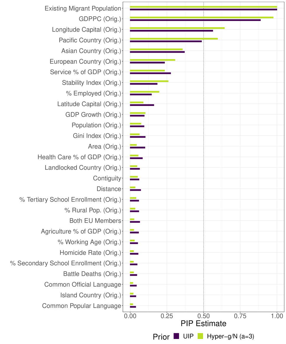
(a) Post. Inclusion Probabilities.

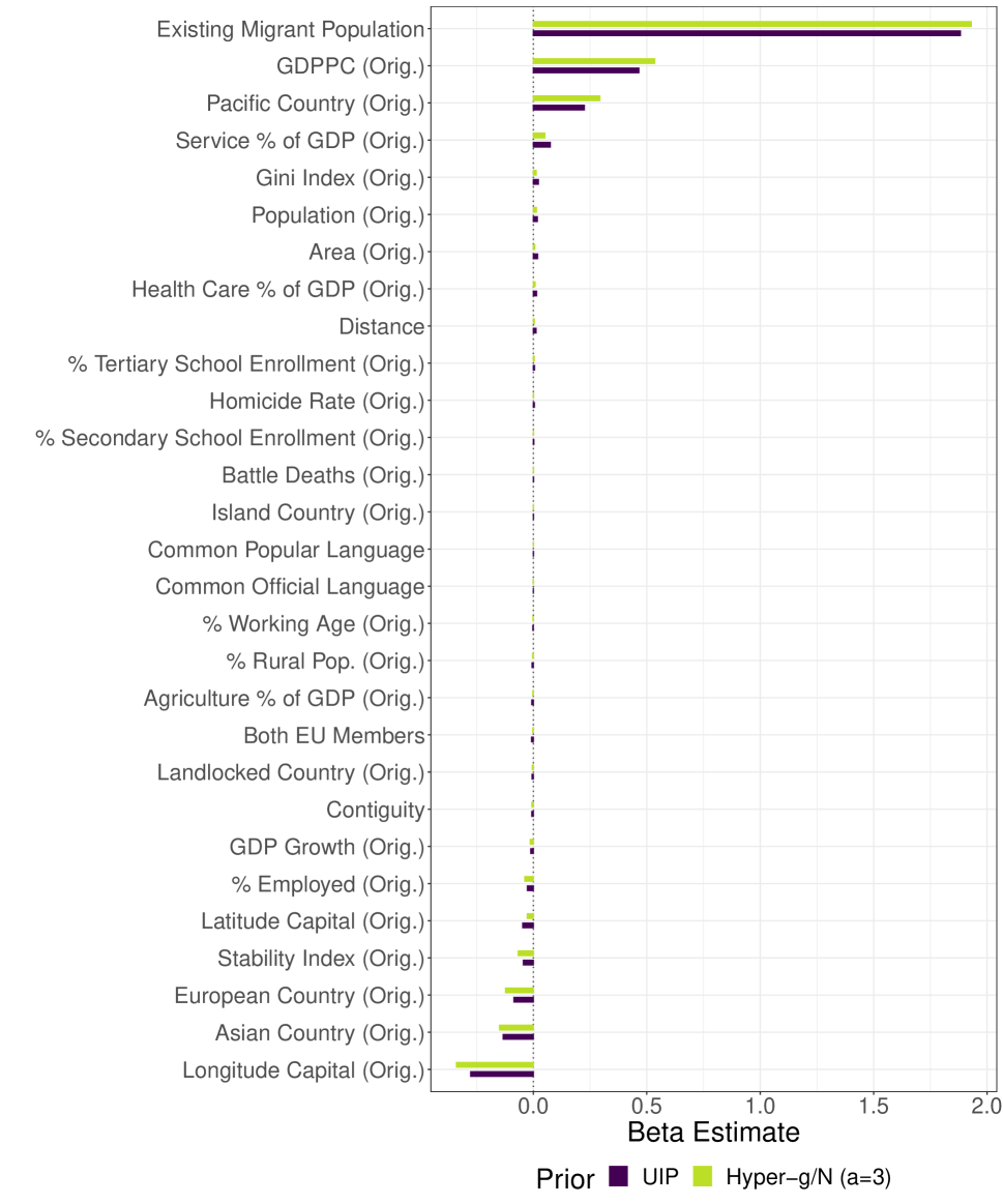
(b) Coefficient Post. Means.

Fig. A11: Estimation Results for Austrian Subset of Bilateral Migration Flow Data.

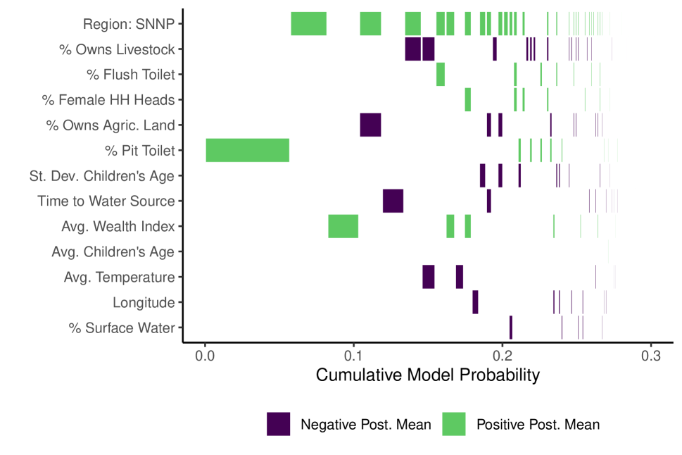
(a) Highest Probability Models.

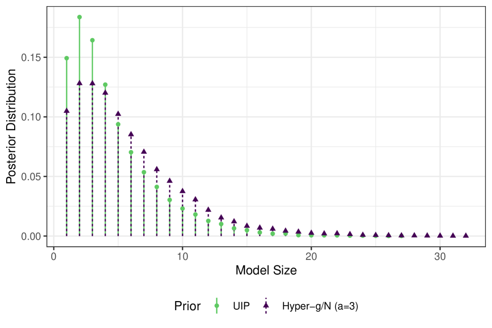
(b) Posterior Distribution of Model Size.

Fig. A12: Estimation Results (Measles Vaccination Data Subset). Highest probability models plot includes variables with estimated $\text{PIP}>0.1$ under unit information prior.

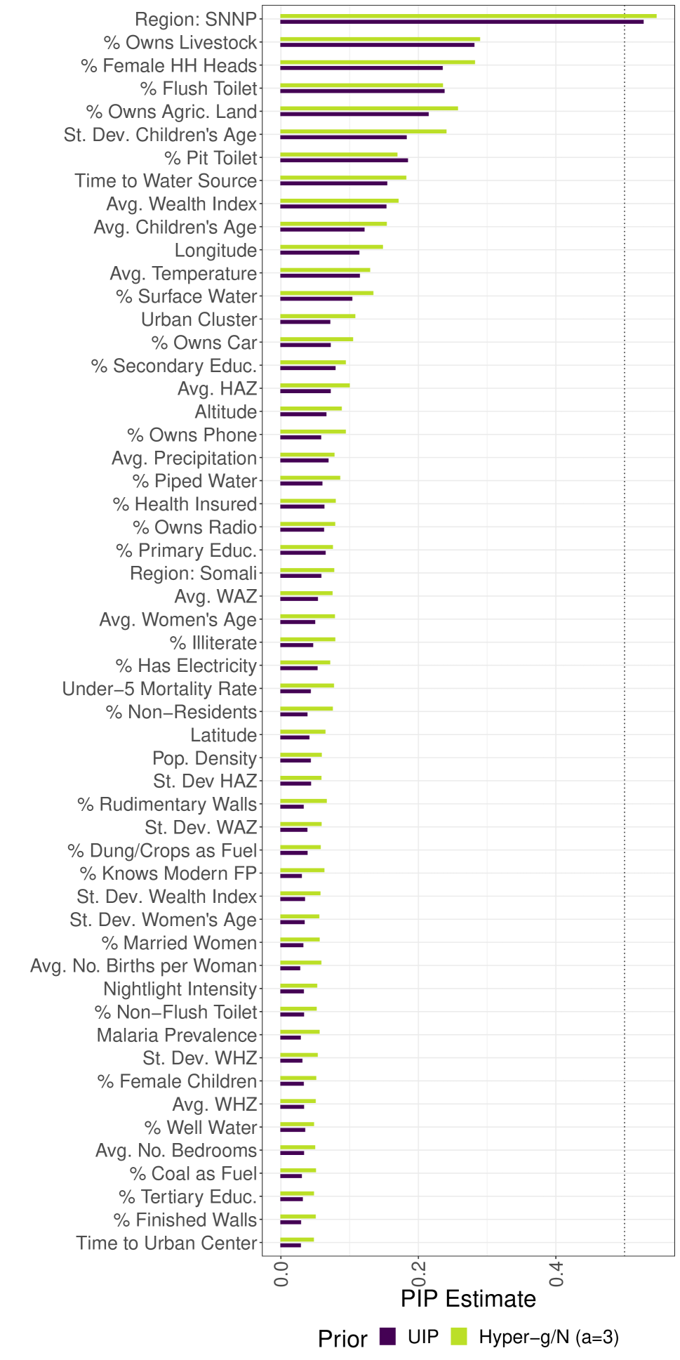
(a) Post. Inclusion Probabilities.

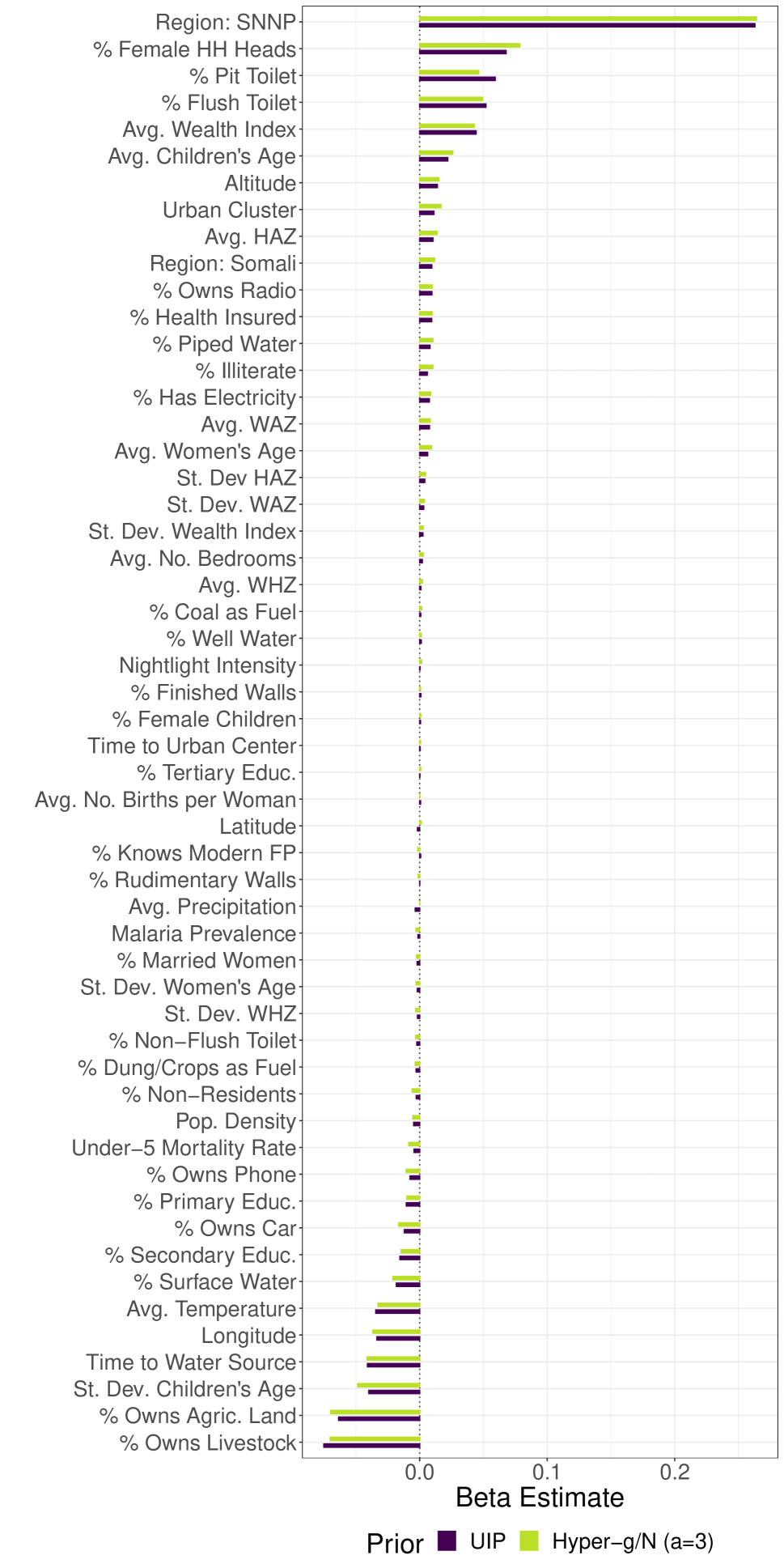
(b) Coefficient Post. Means.

Fig. A13: Estimation Results for Low Vaccination Rate Subset of Measles Vaccination Data.

References

- The multivariate Poisson-log normal distribution. Biometrika 76 (4), pp. 643–653. Cited by: §2.1, §2.2.
- Logistic-normal distributions: some properties and uses. Biometrika 67 (2), pp. 261–272. Cited by: §2.1.
- Criteria for Bayesian model choice with application to variable selection. Annals of Statistics 40 (481), pp. 1550–77. Cited by: §3.
- Bayesian variable selection in high dimensional problems without assumptions on prior model probabilities. technical report Technical Report arXiv:1607.02993v1. Cited by: footnote 2.
- Bayesian Wavelength Selection in Multicomponent Analysis. Journal of Chemometrics 12, pp. 173–82. Cited by: §3.
- Multivariate Bayesian variable selection and prediction. Journal of the Royal Statistical Society: Series B (Statistical Methodology) 60 (3), pp. 627–641. Cited by: §8.
- On fitting the Poisson lognormal distribution to species-abundance data. Biometrics, pp. 101–110. Cited by: §2.1.
- Markov chain Monte Carlo analysis of correlated count data. Journal of Business & Economic Statistics 19 (4), pp. 428–435. Cited by: §2.2, §5.
- Random effects modeling of multiple binomial responses using the multivariate binomial logit-normal distribution. Biometrics 56 (1), pp. 73–80. Cited by: §5.
- Predictive Model Assessment for Count Data. Biometrics 65 (4), pp. 1254–1261. Cited by: §7.3.
- A mixed Poisson–inverse-Gaussian regression model. Canadian Journal of Statistics 17 (2), pp. 171–181. Cited by: §2.1.
- On Bayesian model and variable selection using MCMC. Statistics and Computing 12 (1), pp. 27–36. Cited by: §1.
- Sparse Bayesian modelling of underreported count data. Statistical Modelling 16 (1), pp. 24–46. Cited by: §1.
- Benchmark priors for Bayesian model averaging. Journal of Econometrics 100, pp. 381–427. Cited by: §7.3.
- Auxiliary mixture sampling for parameter-driven models of time series of counts with applications to state space modelling. Biometrika 93 (4), pp. 827–841. Cited by: §1.
- Sampling from the posterior distribution in generalized linear mixed models. Statistics and Computing 7 (1), pp. 57–68. Cited by: §7.3.
- LGM split sampler: an efficient MCMC sampling scheme for latent Gaussian models. Statistical Science 35 (2), pp. 218–233. External Links: Document, Link Cited by: §5.
- An inquiry into the nature of frequency distributions representative of multiple happenings with particular reference to the occurrence of multiple attacks of disease or of repeated accidents. Journal of the Royal statistical society 83 (2), pp. 255–279. Cited by: §2.1.
- In search of lost mixing time: adaptive Markov chain Monte Carlo schemes for Bayesian variable selection with very large p. Biometrika 108 (1), pp. 53–69. Cited by: §5.
- Compound Poisson regression models. In GLIM 82: Proc. Internat. Conf. Generalized Linear Models, pp. 109–121. Cited by: §2.1.
- Bayesian latent gaussian models. In Statistical Modeling Using Bayesian Latent Gaussian Models : With Applications in Geophysics and Environmental Sciences, B. Hrafnkelsson (Ed.), pp. 1–80. External Links: ISBN 978-3-031-39791-2, Document, Link Cited by: §2.
- Bayesian variable selection in a million dimensions. In Proceedings of The 26th International Conference on Artificial Intelligence and Statistics, F. Ruiz, J. Dy, and J. van de Meent (Eds.), Proceedings of Machine Learning Research, Vol. 206, pp. 253–282. External Links: Link Cited by: §1.
- A reference Bayesian test for nested hypotheses and its relationship to the Schwarz criterion. Journal of the American Statistical Association 90 (431), pp. 928–934. Cited by: §6.
- Transdimensional sampling algorithms for Bayesian variable selection in classification problems with many more variables than observations. Journal of Computational and Graphical Statistics 18 (3), pp. 592–612. Cited by: §1, §7.3.
- Mixtures of -priors for Bayesian model averaging with economic applications. Journal of Econometrics 171 (2), pp. 251–66. Cited by: §3, §5, §6.
- On the effect of prior assumptions in Bayesian model averaging with applications to growth regression. Journal of Applied Econometrics 24 (4), pp. 651–674. Cited by: §3, §3.
- Mixtures of priors for Bayesian variable selection. Journal of the American Statistical Association 103 (481), pp. 410–23. Cited by: §3, §6.
- Adaptive MCMC for Bayesian Variable Selection in Generalised Linear Models and Survival Models. Entropy 25 (9). External Links: Link, ISSN 1099-4300, Document Cited by: §5.
- The Barker proposal: Combining robustness and efficiency in gradient-based MCMC. Journal of the Royal Statistical Society, B 84 (2), pp. 496. Cited by: §5.
- Fully Bayes factors with a generalized -prior. Annals of Statistics 39, pp. 2740–2765. Cited by: footnote 2.
- Stochastic search variable selection for log-linear models. Journal of Statistical Computation and Simulation 68 (1), pp. 23–37. Cited by: §8.
- Bayesian inference for logistic models using Pólya–Gamma latent variables. Journal of the American statistical Association 108 (504), pp. 1339–1349. Cited by: §1.
- Examples of adaptive MCMC. Journal of computational and graphical statistics 18 (2), pp. 349–367. Cited by: §5.
- Approximate Laplace approximations for scalable model selection. Journal of the Royal Statistical Society Series B: Statistical Methodology 83 (4), pp. 853–879. Cited by: §1.
- Approximate Bayesian Inference for Latent Gaussian models by using Integrated Nested Laplace Approximations. Journal of the Royal Statistical Society, Ser. B 71, pp. 319–392. Cited by: §2.
- Bayes and empirical Bayes multiplicity adjustment in the variable-selection problem. Annals of Statistics 38, pp. 2587–619. Cited by: §3.
- Multiple-systems analysis for the quantification of modern slavery: classical and Bayesian approaches. Journal of the Royal Statistical Society, A 183 (3), pp. 691–736. Cited by: §8.
- The calculation of posterior distributions by data augmentation. Journal of the American statistical Association 82 (398), pp. 528–540. Cited by: §5.
- Bayesian analysis of Poisson regression with lognormal unobserved heterogeneity: With an application to the patent-R&D relationship. Communications in Statistics—Theory and Methods 39 (10), pp. 1689–1706. Cited by: §2.1, §2.2, §5.
- High resolution age-structured mapping of childhood vaccination coverage in low and middle income countries. Vaccine 36 (12), pp. 1583–1591. Cited by: §7.1.